Spectral determination of semi-regular polygons

Abstract.

Let us say that an $n$-sided polygon is semi-regular if it is circumscriptible and its angles are all equal but possibly one, which is then larger than the rest. Regular polygons, in particular, are semi-regular. We prove that semi-regular polygons are spectrally determined in the class of convex piecewise smooth domains. Specifically, we show that if $\Omega$ is a convex piecewise smooth planar domain, possibly with straight corners, whose Dirichlet or Neumann spectrum coincides with that of an $n$-sided semi-regular polygon $P_{n}$, then $\Omega$ is congruent to $P_{n}$.

1. Introduction

The inverse spectral problem for a bounded planar domain $\Omega_{0}$ is to ascertain whether any domain $\Omega\subset\mathbb{R}^{2}$ with the same spectrum (with, say, Dirichlet boundary conditions) is actually congruent to $\Omega_{0}$. Since Marc Kac reformulated this problem in 1965 as “hearing the shape of a drum” [13], the spectral determination of planar domains (and of more general Riemannian manifolds, with or without boundary) has become a major research topic for analysts and geometers. We recall that the Dirichlet spectrum of a planar domain $\Omega$ is the set (with multiplicities) of numbers $\lambda_{k}$ for which the boundary value problem

$$\Delta u_{k}+\lambda_{k}u_{k}=0\quad\text{in }\Omega\,,\qquad u_{k}|_{\partial\Omega}=0\,,$$

admits a nontrivial solution. The Neumann eigenvalues $\mu_{k}$ of a domain are similarly defined in terms of the boundary value problem

$$\Delta v_{k}+\mu_{k}v_{k}=0\quad\text{in }\Omega\,,\qquad\partial_{\nu}v_{k}=0\,,$$

Most of the existing results of the inverse spectral problem are negative, meaning that they assert that a certain domain or manifold cannot be recovered from its Dirichlet spectrum. In particular, it is known since the 1980s [8] that there are polygons that are isospectral but not isometric. The question of whether there are any smooth or convex planar domains with this property remains open. In the case of Riemannian manifolds it is known that even the local geometry of isospectral manifolds can be different [23].

The list of positive results for the inverse spectral problem remains rather short. In the case of negatively curved manifolds, there are spectral rigidity [6, 10] and compactness results [17], some of which have been recently extended to Anosov surfaces [20]. These compactness results are also valid for planar domains [18, 19]. A major breakthrough has been the proof that, in the class of analytic bounded planar domains with a reflection symmetry, any domain is spectrally determined [26]. This result, which hinges on the computation of all the wave invariants at a closed billiard trajectory formed by a segment that hits the boundary orthogonally at both endpoints, has been extended to higher dimensional domains in [11].

It is very easy to show [13] that the any planar domain with the same Dirichlet spectrum as a disk must be congruent to it. This follows from the facts that disks are the only minimizers of the isoperimetric inequality

$$|\partial\Omega|^{2}\geqslant 4\pi|\Omega|$$

and that the area and length are obtained from the short-time asymptotics of the heat trace

(1) $$h^{\mathrm{Dir}}_{\Omega}(t):=\sum_{k=1}^{\infty}e^{-\lambda_{k}t}\,.$$

The result remains true for balls of any dimension and for Neumann boundary conditions. Quite remarkably, the somewhat reminiscent problem of the spectral determination of round spheres is only known up to dimension 6 [24]. Other than the disks, the only planar domain that is known to be spectrally determined without any symmetry and analyticity assumptions is a family of ovals with four vertices whose isoperimetric quotients are very close to that of a disk [25].

Our objective in this paper is show that regular polygons (that is, those whose angles are all equal and whose sides are all of the same length) are also determined by their Dirichlet or Neumann spectrum in the class of convex piecewise smooth domains. More generally, the result holds for the polygons that we will call semi-regular, meaning circumscriptible polygons whose angles are all equal but possibly one, which must then be larger than the rest:

Theorem 1.

Let $P_{n}$ be a semi-regular $n$-sided polygon. If $\Omega$ is a convex piecewise smooth bounded planar domain, possibly with straight corners, and its Dirichlet or Neumann spectrum coincides with that of $P_{n}$, then $\Omega$ is congruent to $P_{n}$.

Of course, a planar domain is said to be piecewise smooth if its boundary is a $C^{\infty}$ curve but possibly at a finite number of points, which we call corner points. We assume that the corners are straight, i.e., that the boundary is flat in a small neighborhood of each corner point. As a side remark, notice that, when considering the inverse spectral problem for regular polygons, it is essential to allow for piecewise smooth domains because a domain with corners cannot be isospectral to a domain with smooth boundary [15].

Let us discuss the main ideas of the proof of the theorem in the case of Dirichlet boundary conditions, the Neumann case being completely analogous. The key step of the proof is to prove the result for convex polygons, that is, to show that if $P$ is a polygon isospectral to an $n$-sided semi-regular polygon $P_{n}$, then $P$ and $P_{n}$ are congruent. The reason is that the asymptotic behavior at 0 of the heat trace (1) of a piecewise domain $\Omega$ with $m$ straight corners is, as shown in Proposition 8 using results available in the literature,

$$h_{\Omega}^{\mathrm{Dir}}(t)=\frac{|\Omega|}{4\pi t}-\frac{|\partial\Omega|}{8\sqrt{\pi t}}+\frac{1}{12\pi}\bigg{(}\int_{\partial\Omega}\kappa\,ds+\sum_{k=1}^{m}\frac{\pi^{2}-\theta_{k}^{2}}{2\theta_{k}}\bigg{)}+\frac{\sqrt{t}}{256\sqrt{\pi}}\int_{\partial\Omega}\kappa^{2}\,ds+O(t)\,,$$

where $\theta_{k}\in(0,2\pi)$ is the interior angle at the $j^{\text{th}}$ corner point and $\kappa$ is the curvature of the boundary at each differentiable point. From the expression of the term of order $\sqrt{t}$ it is not hard to see that the boundary of $\Omega$ must be flat, which means that $\Omega$ must indeed be a polygon. Notice that the only reason for which we have made the technical assumption that the corners of $\Omega$ are straight is simply that the fourth coefficient of the asymptotic expansion of the heat trace has apparently not yet been computed for domains with non-straight corners. In the case of straight corners and Dirichlet boundary boundary conditions, the result was first obtained (but not published) by Dan Ray, as referenced by Kac [13] and later by Cheeger [4], while for Neumann boundary conditions the result has appeared only very recently [16].

To establish the result for polygons we derive a new characterization of semi-regular polygons as extremizers (in the space of convex polygons whose number of sides is not fixed) of a kind of constrained isoperimetric inequality which, to our best knowledge, had not appeared in the literature before. The constraint involves a third geometric quantity that is a spectral invariant and whose expression, which is highly nontrivial from a geometric standpoint, can only be guessed using spectral-theoretic methods. Let us recall that an $n$-sided regular polygon is the $n$-gon with fixed area and minimal perimeter, but regular polygons are not extremizers of the isoperimetric inequality when one allows for polygons with an arbitrary number of sides, and one does not know how to find the number of sides of a polygon using spectral invariants. Hence the key advantage of our isoperimetric-type characterization of regular (and, more generally, semi-regular) polygons is that it enables us to characterize an $n$-sided semi-regular polygon among polygons with an arbitrary number of sides. It should be noticed that the hypothesis that the domains are convex is only used in this part of the proof.

Incidentally, let us recall that, for a fixed number of sides, the problem becomes effectively finite-dimensional, so finer results can sometimes be proved. For example, it is easy to prove that any rectangle is characterized among rectangles by its spectrum. The same result is true in the case of triangles, but the proof is much harder (see [7] for the original proof based on wave invariants and [9] for a simpler proof that only needs the heat kernel). Likewise, trapezoids have been recently shown [12] to be determined by their Neumann spectrum within the class of trapezoids. The proof makes essential use of wave invariants to obtain an additional geometric quantity, which does not appear in the heat trace and is crucially used to determine the parameters that characterize an arbitrary trapezoid.

The paper consists of two sections corresponding to the two parts of the proof that we have described above. The proof that any polygon isospectral with a semi-regular polygon is indeed congruent to it, which is the heart of the paper, is presented in Section 2. The proof of Theorem 1 then follows after showing that any domain isospectral with a polygon must be a polygon, which is established in Section 3.

2. Semi-Regular polygons as maximizers

Our objective in this section is to show that any $m$-sided polygon $P$ that is isometric to an $n$-sided semi-regular polygon is in fact congruent to it.

For this we will rely on the well known fact (see [2] for a transparent derivation) that the asymptotic behavior of the heat kernel of a polygon $P$ can be completely characterized modulo exponentially small terms as

$$h_{P}^{\mathrm{Dir}}(t)=\frac{|P|}{4\pi t}-\frac{|\partial P|}{8\sqrt{\pi t}}+\frac{S(P)}{24\pi}+O(e^{-c/t})\,,$$

where $|P|$ and $|\partial P|$ respectively denote the area and perimeter of $P$ and

$$S(P):=\sum_{k=1}^{m}\frac{\pi^{2}-\theta_{k}^{2}}{\theta_{k}}\,.$$

In the Neumann case, where the heat trace is defined as

$$h^{\mathrm{Neu}}(t):=\sum_{k=1}^{\infty}e^{-\mu_{k}t}\,,$$

the formulas are identical modulo a sign reversal [16]:

$$h_{P}^{\mathrm{Neu}}(t)=\frac{|P|}{4\pi t}+\frac{|\partial P|}{8\sqrt{\pi t}}+\frac{S(P)}{24\pi}+O(e^{-c/t})\,,$$

Hence our goal in this section is to characterize semi-regular polygons as the maximizers of a functional that one can construct using only the three quantities that appear in the heat trace asymptotics of a polygon: the area, the length and the function $S(P)$. Furthermore, we can use dilations to restrict our attention to polygons with unit perimeter. This leaves us just the area $|P|$ and the function $S(P)$, and we will define the maximization problem as follows:

Definition.

We will say that a convex polygon $P$ with unit perimeter is a maximizer if for every convex polygon $Q$ with unit perimeter and $S(Q)=S(P)$ one has $|Q|\leqslant|P|$.

Figure 1. Plot of the quantities $(|P|,S(P))$ for 20,000 randomly generated convex polygons of unit perimeter. The dashed line corresponds to the semiregular 4-gons, the endpoints being the equilateral triangle and the square.

Notice that a maximizer is an extremizer of the isoperimetric quotient among polygons subject to the constraint that the value of the function $S$ is fixed. The key ingredient in the proof of Theorem 1 is the following result, which shows that semi-regular polygons are the only maximizers. For the benefit of the reader, before presenting the statement and proof of this result it is worth to illustrate this result with some numerical results to get some intuition. In Figure 1 we have plotted the values $(S(P),|P|)$ for 20,000 randomly generated convex polygons of unit perimeter that we have obtained using Monte Carlo simulations. On top of this we have plotted the curve $(S(P),|P|)$ corresponding to the semi-regular polygons.

Theorem 2.

A convex $n$-sided polygon of unit perimeter is a maximizer if and only if it is circumscriptible and all its angles are equal but possibly one, which must then be larger than the rest. Moreover, if $P$ and $Q$ are two non-congruent polygons as above, possibly with a different number of sides, then $S(P)\neq S(Q)$.

Proof.

We will show that if a polygon $P$ is a maximizer, then it needs to be of that form, and that the maximizer is completely determined by the value of the function $S$.

The first observation is that while looking for maximizers we can restrict ourselves to the class of circumscriptible polygons. This is by a classical result of L’Huilier [14], extended to the case of polygons on the sphere by Steiner [22], which asserts that among all convex $n$-sided polygons of unit perimeter with given angles, only the one circumscribed to a circle has the largest area.

We can therefore write all the quantities in terms of the interior angles of the polygon $\theta_{1},\theta_{2},\ldots,\theta_{n}$, now assumed to be circumscribed to a circle (see Figure 2), which yields the following formulas after imposing that $|\partial P|=1$:

$$S(P)=\sum_{k=1}^{n}\frac{\pi^{2}-\theta_{k}^{2}}{\theta_{k}},\quad|P|=\frac{1}{4}\left(\sum_{k=1}^{n}\cot\frac{\theta_{k}}{2}\right)^{-1}$$

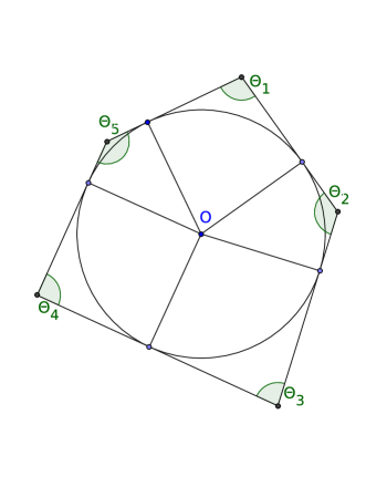
Figure 2. A circumscriptible pentagon

We want to fix the value of $S(P)$, which for convenience we will denote by $4\pi\frac{s-1}{s-2}$ with $s>2$. The reason for choosing this normalization is that the value of the function $S$ on the regular $n$-sided polygon is precisely $4\pi\frac{n-1}{n-2}$. We also know that the sum of the angles of an $n$-sided polygon must satisfy

(2) $$\sum_{i=1}^{n}\theta_{i}=(n-2)\pi.$$

We will consider the following problem, where the unknown is the set of numbers $(\theta_{1},\dots,\theta_{n})\in(0,\pi)^{n}$ subject to the constraints that correspond to setting

$$S(P)=4\pi\frac{s-1}{s-2}$$

and imposing the geometric condition (2):

Problem $\mathrm{P}_{s,n}$.

Maximize the quantity

$$\left(\sum_{k=1}^{n}\cot\frac{\theta_{k}}{2}\right)^{-1}$$

with $(\theta_{1},\dots,\theta_{n})\in(0,\pi)^{n}$ subject to the constraints that

$$\sum_{k=1}^{n}\frac{1}{\theta_{k}}=\frac{1}{\pi}\left(n+\frac{2s}{s-2}\right)\,,\qquad\sum_{i=1}^{n}\theta_{i}=(n-2)\pi\,.$$

We will show that there is a unique solution to this problem, which defines a circumscriptible polygon of $\lceil s\rceil$ sides whose angles are all equal but possibly one, which is then larger than the rest. To do so, we proceed by induction in $n$.

We start doing the base case $n=\lceil s\rceil$, as $n$ cannot be smaller than $\lceil s\rceil$ because of the isoperimetric inequality for polygons. Using the inequality [5, Remark 1.4, Corollary 1.6], all we have to do in this case is to check that the function

$$g(x):=f^{\prime}(x^{-\frac{1}{2}})$$

is concave in the interval $\left(\pi^{-2},\infty\right)$, where

$$f(x):=\cot\frac{x}{2}\,.$$

Since

$$g(x)=\frac{1}{\cos x^{-\frac{1}{2}}-1}\,,$$

its second derivative is

$$g^{\prime\prime}(x)=-\frac{2+\cos x^{-\frac{1}{2}}-3x^{\frac{1}{2}}\sin x^{-\frac{1}{2}}}{16x^{3}\sin^{4}(\frac{1}{2}x^{-\frac{1}{2}})}.$$

Thus to prove that the function $g$ is concave it suffices to show that

$$z\,(2+\cos z)-3\sin z>0$$

for all $z\in(0,\pi)$.

Using a sixth order Taylor expansion one readily sees that, for all $z\in(0,\pi)$,

$$z\,(2+\cos z) =z\left(3-\frac{z^{2}}{2}+\frac{z^{4}}{24}-\frac{z^{6}}{720}+\frac{1}{5040}\int_{0}^{z}(z-\zeta)^{6}\sin\zeta\,d\zeta\right)$$

$$>z\left(3-\frac{z^{2}}{2}+\frac{z^{4}}{24}-\frac{z^{6}}{720}\right)\,,$$

and by a similar argument

$$3\sin z<3z-\frac{z^{3}}{2}+\frac{z^{5}}{40}$$

on $(0,\pi)$. This ensures that, for all $z$ in $(0,\pi)$,

$$z\,(2+\cos z)-3\sin z >\frac{z^{5}}{60}-\frac{z^{7}}{720},$$

which is strictly positive on this interval. The case $n=\lceil s\rceil$ then follows.

We now move on to establish the inductive step. We can therefore take some $n$, assume that the only maximizer of Problem P${}_{s,n^{\prime}}$ for any $n^{\prime}<n$ is the aforementioned polygon, and show that the same remains true for Problem P_s,n. To this end we shall next show that we can reduce Problem P_s,n to a problem of the form P${}_{s,n^{\prime}}$ with $n^{\prime}<n$.

Using Lagrange multipliers, we need to minimize the function

$$F(\theta_{1},\ldots,\theta_{n},\lambda_{1},\lambda_{2}):=\sum_{k=1}^{n}\cot\frac{\theta_{k}}{2}+\lambda_{1}\left(\sum_{k=1}^{n}\frac{1}{\theta_{k}}-\frac{n}{\pi}-\frac{2s}{\pi(s-2)}\right)\\ +\lambda_{2}\left(\sum_{i=1}^{n}\theta_{i}-(n-2)\pi\right)$$

whose minima for fixed $(\lambda_{1},\lambda_{2})$ and $(\theta_{1},\dots,\theta_{n})\in(0,\pi)^{n}$ must be either attained at interior critical points or lie on the boundary.

We first deal with the boundary case. There are two possibilities: either $\theta_{i}=0$ for some $i$ or $\theta_{i}=\pi$ for some $i$. In the former case the function $F$ will go to $+\infty$ and thus it will not be a minimum. In the latter, having a minimum at a point of the form

(3) $$(\theta_{1},\ldots,\theta_{i-1},\pi,\theta_{i+1},\ldots,\theta_{n})$$

of Problem P_s,n is equivalent to have a minimum $(\theta_{1},\ldots,\theta_{i-1},\theta_{i+1},\ldots,\theta_{n})$ of Problem P_s,n-1, which is ruled out by the induction hypothesis.

Therefore, it boils down to controlling the interior critical points of the function $F$. Taking the partial derivative with respect to $\theta_{i}$, we infer that if there is a local minimum at $(\theta_{1},\dots,\theta_{n})$ then one necessarily has, for $1\leqslant i\leqslant n$,

$$0=\frac{\partial F}{\partial\theta_{i}}(\theta_{1},\dots,\theta_{n},\lambda_{1},\lambda_{2})=\Phi(\theta_{i},\lambda_{1},\lambda_{2})\,,$$

where

$$\Phi(z,\lambda_{1},\lambda_{2}):=-\frac{1}{2\sin^{2}\frac{z}{2}}-\frac{\lambda_{1}}{z^{2}}+\lambda_{2}\,.$$

The key observation here is that one gets the same equation for all the angles, which only depends on one of the variables at a time and on the Lagrange parameters. Furthermore, it was proved in [9, Lemma 1(b)] that the function $\Phi(\cdot,\lambda_{1},\lambda_{2})$ has at most two zeros on the interval $(0,\pi)$ for any value of $(\lambda_{1},\lambda_{2})$. This implies that if $(\theta_{1},\dots,\theta_{n})$ is a critical point then the angles $\theta_{i}$ can take at most two distinct values.

Let us assume that the two distinct values are $\bar{\theta}_{1}$ and $\bar{\theta}_{2}$ and that there are $k$ and $n-k$ copies of each angle respectively. Problem P_s,n is reduced to the following:

Problem $\mathrm{P}^{\prime}_{s,n}$.

Maximize the function

$$\left(k\cot\frac{\bar{\theta}_{1}}{2}+(n-k)\cot\frac{\bar{\theta}_{2}}{2}\right)^{-1}$$

with $(\bar{\theta}_{1},\bar{\theta}_{2})\in(0,\pi)^{2}$ subject to the constraints that

$$\frac{k}{\bar{\theta}_{1}}+\frac{n-k}{\bar{\theta}_{2}}=\frac{1}{\pi}\left(n+\frac{2s}{s-2}\right)\,,\quad k\bar{\theta}_{1}+(n-k)\bar{\theta}_{2}=(n-2)\pi$$

Solving the constraints for $(\bar{\theta}_{1},\bar{\theta}_{2})$ in terms of $(k,n)$ and plugging the resulting expressions into the function we want to maximize yields very complicated formulas, so instead we will solve for $(k,n)$ as functions of $(\bar{\theta}_{1},\bar{\theta}_{2})$. This is much simpler because the constraints depend linearly on $k$ and $n$, so we get

$$n(s,\bar{\theta}_{1},\bar{\theta}_{2}) =\frac{2(s-2)\pi^{2}-2\bar{\theta}_{1}\bar{\theta}_{2}s}{(s-2)(\pi-\bar{\theta}_{1})(\pi-\bar{\theta}_{2})}\,,$$

$$k(s,\bar{\theta}_{1},\bar{\theta}_{2}) =\frac{2\bar{\theta}_{1}(\bar{\theta}_{2}s-(s-2)\pi)}{(s-2)(\bar{\theta}_{2}-\bar{\theta}_{1})(\pi-\bar{\theta}_{1})}\,.$$

This allows us to get rid of the constraints and minimize the objective function

$$G_{s}(\bar{\theta}_{1},\bar{\theta}_{2}):=k(s,\bar{\theta}_{1},\bar{\theta}_{2})\cot\frac{\bar{\theta}_{1}}{2}+(n(s,\bar{\theta}_{1},\bar{\theta}_{2})-k(s,\bar{\theta}_{1},\bar{\theta}_{2}))\cot\frac{\bar{\theta}_{2}}{2}$$

with $(\bar{\theta}_{1},\bar{\theta}_{2})\in(0,\pi)^{2}$.

We first argue that $k$ and $n-k$ must be both larger than or equal to 1. Indeed, if one assumes that $k=0$, that implies that $\bar{\theta}_{2}=\frac{n-2}{n}\pi$, with solution $n=s$ whenever $s$ is an integer and no solution otherwise. This case is discarded because we are assuming that $n\geqslant\lceil s\rceil+1$. A similar argument shows that $n-k\geqslant 1$.

Because of the symmetries of the problem (that is, the fact that exchanging $\bar{\theta}_{1}$ for $\bar{\theta}_{2}$ is equivalent to exchanging $k$ for $n-k$), it is enough to consider the case $\bar{\theta}_{1}\geqslant\bar{\theta}_{2}$. The next step is to reduce the region where critical points can lie. First, we notice that $k(s,\bar{\theta}_{1},\bar{\theta}_{2})\geqslant 0$ if and only if

(4) $$\bar{\theta}_{2}\leqslant\frac{s-2}{s}\pi\,,$$

and straightforward calculations show that

$$k(s,\bar{\theta}_{1},\bar{\theta}_{2})\leqslant n(s,\bar{\theta}_{1},\bar{\theta}_{2})$$

if and only if

(5) $$\bar{\theta}_{1}\geqslant\frac{s-2}{s}\pi\,.$$

If we further impose the condition

$$n(s,\bar{\theta}_{1},\bar{\theta}_{2})\geqslant s+1\,,$$

a short computation shows that

(6) $$\bar{\theta}_{1}\geqslant h(s,\bar{\theta}_{2})\,,$$

where

$$h(s,\bar{\theta}_{2}) :=\frac{\pi(s-2)(\pi(s-1)-\bar{\theta}_{2}(1+s))}{2\bar{\theta}_{2}+(s+1)(\pi(s-2)-s\bar{\theta}_{2})}\,.$$

Notice that $h(s,\bar{\theta}_{2})$ is an increasing function of $\bar{\theta}_{2}$ in the interval $\left[0,\frac{s-2}{s}\pi\right]$, so this readily gives the uniform bound

$$\bar{\theta}_{1}\geqslant h(s,0)=\frac{s-1}{s+1}\pi$$

Due to the constraints on $(\bar{\theta}_{1},\bar{\theta}_{2})$ imposed by (4)–(6), we will look for maximizers of Problem P${}_{s,n}^{\prime}$ in the bounded planar domain ${\mathcal{S}}_{s}$ whose boundary is given by the segments

$$\Gamma^{{\mathcal{S}}_{s}}_{1} :=\bigg{\{}\bar{\theta}_{1}=\frac{(s^{2}-s-2)\pi}{s^{2}+s-2}-\frac{4\pi^{2}(s-2)}{(s^{2}+s-2)(\bar{\theta}_{2}(s^{2}+s-2)+\pi(-s^{2}+s+2))},$$

$$\qquad\qquad\qquad\qquad\qquad\qquad\qquad\qquad\qquad\qquad\qquad\qquad\qquad\quad\;\bar{\theta}_{2}\in\left[0,\frac{s-2}{s}\pi\right]\bigg{\}}$$

$$\Gamma^{{\mathcal{S}}_{s}}_{2} :=\left\{\bar{\theta}_{1}\in\left[\frac{s-1}{s+1}\pi,\;\pi\right],\bar{\theta}_{2}=0\right\},\quad\Gamma^{{\mathcal{S}}_{s}}_{3}:=\left\{\bar{\theta}_{1}=\pi,\;\left[0,\frac{s-2}{s}\pi\right]\right\}.$$

For computational purposes, it is often convenient to consider the larger region ${\mathcal{R}}_{s}\supset{\mathcal{S}}_{s}$ (see Figure 3) that is bounded by the segments

$$\Gamma^{{\mathcal{R}}_{s}}_{1} :=\left\{\bar{\theta}_{1}=\frac{s-1}{s+1}\pi,\;\bar{\theta}_{2}\in\left[0,\frac{s-2}{s}\pi\right]\right\},\quad\Gamma^{{\mathcal{R}}_{s}}_{2}:=\left\{\bar{\theta}_{1}\in\left[\frac{s-1}{s+1}\pi,\pi\right],\;\bar{\theta}_{2}=0\right\}$$

$$\Gamma^{{\mathcal{R}}_{s}}_{3} :=\left\{\bar{\theta}_{1}=\pi,\;\bar{\theta}_{2}\in\left[0,\frac{s-2}{s}\pi\right]\right\},\quad\Gamma^{{\mathcal{R}}_{s}}_{4}:=\left\{\bar{\theta}_{1}\in\left[\frac{s-1}{s+1}\pi,\;\pi\right],\bar{\theta}_{2}=\frac{s-2}{s}\pi\right\}\,.$$

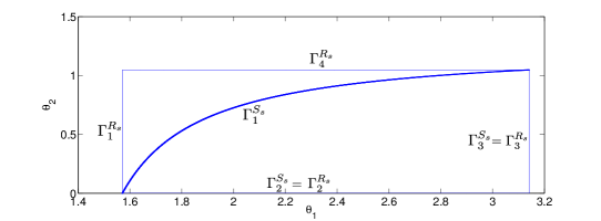
Figure 3. The regions ${\mathcal{R}}_{3}$ and ${\mathcal{S}}_{3}$

We start by showing that the function $G_{s}$ does not have any critical points in the interior of ${\mathcal{R}}_{s}$. The key fact is contained in the following proposition, whose rather involved proof contains two auxiliary lemmas:

Proposition 3.

The derivative of the function $G_{s}$ with respect to the first variable satisfies

$$\partial_{\bar{\theta}_{1}}G_{s}(\bar{\theta}_{1},\bar{\theta}_{2})>0 \qquad\text{in the interior of }{\mathcal{R}}_{s}\,,$$

$$\partial_{\bar{\theta}_{1}}G_{s}(\bar{\theta}_{1},\bar{\theta}_{2})>0 \qquad\text{on }\Gamma^{{\mathcal{R}}_{s}}_{2}\,,$$

$$\partial_{\bar{\theta}_{1}}G_{s}(\bar{\theta}_{1},\bar{\theta}_{2})=0 \qquad\text{on }\Gamma^{{\mathcal{R}}_{s}}_{4}\,.$$

Proof.

Taking the derivative yields

$$\partial_{\bar{\theta}_{1}}G_{s}(\bar{\theta}_{1},\bar{\theta}_{2}) =\frac{(s-2)\pi-\bar{\theta}_{2}s}{(\bar{\theta}_{1}-\bar{\theta}_{2})^{2}(s-2)(\pi-\bar{\theta}_{2})}\,\widetilde{G}_{s}(\bar{\theta}_{1},\bar{\theta}_{2})\,,$$

where

$$\widetilde{G}_{s}(\bar{\theta}_{1},\bar{\theta}_{2}):=\frac{1}{(\pi-\bar{\theta}_{1})^{2}}\bigg{[}2\bar{\theta}_{2}(\bar{\theta}_{1}-\pi)^{2}\cot\frac{\bar{\theta}_{2}}{2}\\ +(\pi-\bar{\theta}_{2})\csc^{2}\frac{\bar{\theta}_{1}}{2}\big{(}\bar{\theta}_{1}(\bar{\theta}_{1}-\bar{\theta}_{2})(\bar{\theta}_{1}-\pi)+(\bar{\theta}_{1}^{2}-\bar{\theta}_{2}\pi)\sin\bar{\theta}_{1}\big{)}\bigg{]}$$

This automatically shows that the derivative vanishes on $\Gamma^{{\mathcal{R}}_{s}}_{4}$. Since the first factor is always positive in the interior of ${\mathcal{R}}_{s}$ and on $\Gamma^{{\mathcal{R}}_{s}}_{2}$, we only need to show that $\widetilde{G}_{s}(\bar{\theta}_{1},\bar{\theta}_{2})>0$ in ${\mathcal{R}}_{s}$.

We will next show that $\widetilde{G}_{s}$ is increasing in $\bar{\theta}_{1}$, which will be enough to finish the proof once we show that $\widetilde{G}_{s}(\frac{s-1}{s+1}\pi,\bar{\theta}_{2})>0$. We start by taking a derivative with respect to $\bar{\theta}_{1}$, which gives us

$$\partial_{\bar{\theta}_{1}}\widetilde{G}_{s}(\bar{\theta}_{1},\bar{\theta}_{2}) =\left[(\bar{\theta}_{1}-\bar{\theta}_{2})(\pi-\bar{\theta}_{2})\csc^{2}\left(\frac{\bar{\theta}_{1}}{2}\right)\right]\big{(}T_{1}(\bar{\theta}_{1})-T_{2}(\bar{\theta}_{1})\big{)}\,,$$

where

$$T_{1}(x) :=\frac{x}{\pi-x}\cot\frac{x}{2}\,,$$

$$T_{2}(x) :=-\frac{2\pi}{(\pi-x)^{3}}(x-\pi+\sin x)\,.$$

The factor in square brackets is always strictly positive. We shall now show that the second factor is also strictly positive. We remark that this factor, that is $T_{1}(\bar{\theta}_{1})-T_{2}(\bar{\theta}_{1})$, is independent of $s$ and $\bar{\theta}_{2}$, so we are left with two functions of just one variable.

Lemma 4.

$T_{1}(x)\geqslant T_{2}(x)$ for all $x\in[0,\pi]$, with equality only at $x=0$.

Proof.

An easy computation shows that $T_{1}(0)=T_{2}(0),T_{1}^{\prime}(0)=T_{2}^{\prime}(0)$. We will show that $T_{1}^{\prime\prime}(x)>0$ and $T_{2}^{\prime\prime}(x)\leqslant 0$ for all $x\in[0,\pi]$.

Expanding the cotangent in partial fractions [1, 4.3.91] as

$$\cot z=\frac{1}{z}+2z\sum_{k\geqslant 1}\frac{1}{z^{2}-(k\pi)^{2}}$$

we get

$$T_{1}(x) =\frac{2}{\pi-x}+\sum_{k\geqslant 1}\frac{4x^{2}}{(\pi-x)(x^{2}-(2k\pi)^{2})}\,.$$

Taking two derivatives we obtain, for $x\in(0,\pi)$,

$$T_{1}^{\prime\prime}(x) =\frac{4}{(\pi-x)^{3}}+\sum_{k\geqslant 1}\bigg{(}-\frac{8}{(4k^{2}-1)(\pi-x)^{3}}-\frac{8k}{(x-2k\pi)^{3}(2k-1)}$$

$$\qquad\qquad\qquad\qquad\qquad\qquad\qquad\qquad\qquad\qquad-\frac{8k}{(x+2k\pi)^{3}(2k+1)}\bigg{)}$$

$$=-\sum_{k\geqslant 1}\left(\frac{8k}{(x-2k\pi)^{3}(2k-1)}+\frac{8k}{(x+2k\pi)^{3}(2k+1)}\right)$$

(7) $$=\sum_{k\geqslant 1}\frac{32k^{2}(4k^{2}\pi^{3}+12k^{2}\pi^{2}x+3\pi x^{2}+x^{3})}{(2k-1)(1+2k)(2k\pi-x)^{3}(2k\pi+x)^{3}}>0,$$

where we have used that the first term of the infinite sum is telescopic and cancels out with the term which is independent of $k$.

A straightforward computation yields

$$T_{2}^{\prime\prime}(x) =2\pi\frac{6(\pi-x)(1-\cos x)-(12-(\pi-x)^{2})\sin x}{(\pi-x)^{5}}\,,$$

so obviously $T_{2}^{\prime\prime}(x)\leqslant 0$ if and only if

$$6(\pi-x)(1-\cos x)-(12-(\pi-x)^{2})\sin x \leqslant 0\,.$$

When written in terms of the variable $\frac{x}{2}$, this can be readily shown to be equivalent to demanding that

(8) $$\tan\frac{x}{2}\leqslant\frac{12-(\pi-x)^{2}}{6(\pi-x)}=\frac{2}{\pi-x}-\frac{\pi-x}{6}\,.$$

The Taylor expansion of this function at $\pi$ can be read off [1, 4.3.70]:

$$\tan\frac{x}{2} =\frac{2}{\pi-x}-2\sum_{j\geqslant 0}\frac{(-1)^{j+1}(x-\pi)^{2j+1}}{(2j+2)!}B_{2j+2}$$

$$=\frac{2}{\pi-x}-\frac{\pi-x}{6}-2\sum_{j\geqslant 1}\frac{(-1)^{j}(\pi-x)^{2j+1}}{(2j+2)!}B_{2j+2}\,.$$

Here $B_{n}$ denotes the $n$th Bernoulli number. Since $(-1)^{j}B_{2j+2}>0$ for every $j\geqslant 1$, we infer (8) and the lemma follows. ∎

The last step is to show that $\widetilde{G}_{s}(\frac{s-1}{s+1}\pi,\bar{\theta}_{2})>0$. To this end we will define the auxiliary one-variable function

$$\widehat{G}_{s}(\bar{\theta}_{2}):=\widetilde{G}_{s}\Big{(}\frac{s-2}{s}\pi,\bar{\theta}_{2}\Big{)}\,\frac{2s\pi}{\pi-\bar{\theta}_{2}}\,.$$

A short computation shows that

$$\widehat{G}_{s}^{\prime}(\bar{\theta}_{2})=4s\pi T_{1}^{\prime}(\bar{\theta}_{2})+(s-2)\pi s\sec^{2}\frac{\pi}{s}-s^{3}\tan\frac{\pi}{s}$$

and

$$\widehat{G}_{s}^{\prime\prime}(\bar{\theta}_{2})=4s\pi T_{1}^{\prime\prime}(\bar{\theta}_{2})\,,$$

which is positive on $(0,\pi)$ by (7). As moreover

$$\widehat{G}_{s}\Big{(}\frac{s-2}{s}\pi\Big{)}=\widehat{G}_{s}^{\prime}\Big{(}\frac{s-2}{s}\pi\Big{)}=0\,,$$

we infer that $\widehat{G}_{s}(\bar{\theta}_{2})>0$ for all $\bar{\theta}_{2}<\frac{s-2}{s}\pi$, as we wanted to prove. Proposition 3 then follows. ∎

Two immediate consequences of Proposition 3 are that there are no critical points of $G_{s}$ in the interior of ${\mathcal{S}}_{s}$ and that the minimum of $G_{s}$ in ${\mathcal{R}}_{s}$ is attained on $\Gamma^{{\mathcal{R}}_{s}}_{1}\cup\Gamma^{{\mathcal{R}}_{s}}_{4}$. Furthermore,

(9) $$\min_{(\bar{\theta}_{1},\bar{\theta}_{2})\in{\mathcal{S}}_{s}}G_{s}(\bar{\theta}_{1},\bar{\theta}_{2})=\min_{(\bar{\theta}_{1},\bar{\theta}_{2})\in\Gamma_{1}^{{\mathcal{S}}_{s}}}G_{s}(\bar{\theta}_{1},\bar{\theta}_{2})\geqslant\min_{(\bar{\theta}_{1},\bar{\theta}_{2})\in\Gamma_{1}^{{\mathcal{R}}_{s}}}G_{s}(\bar{\theta}_{1},\bar{\theta}_{2})\,,$$

with equality if and only if the RHS minimum is attained at

$$(\bar{\theta}_{1},\bar{\theta}_{2})=\Big{(}\frac{s-1}{s+1}\pi,0\Big{)}\quad\text{or}\quad(\bar{\theta}_{1},\bar{\theta}_{2})=\Big{(}\frac{s-1}{s+1}\pi,\frac{s-2}{s}\pi\Big{)}\,.$$

In either of the two cases, the minimum over ${\mathcal{S}}_{s}$ is attained at only one single point, respectively:

$$(\bar{\theta}_{1},\bar{\theta}_{2})=\Big{(}\frac{s-1}{s+1}\pi,0\Big{)}\quad\text{or}\quad(\bar{\theta}_{1},\bar{\theta}_{2})=\Big{(}\pi,\frac{s-2}{s}\pi\Big{)}\,.$$

We shall next show that the minimum is indeed attained at the latter point:

Lemma 5.

Let

$$g_{s}(\bar{\theta}_{2}) :=G_{s}\Big{(}\frac{s-1}{s+1}\pi,\bar{\theta}_{2}\Big{)}$$

be the restriction of $G_{s}$ to the boundary $\Gamma_{1}^{{\mathcal{R}}_{s}}$. The minimum of $g_{s}$ in the interval $[0,\frac{s-2}{s}\pi]$ is attained at the endpoint $\bar{\theta}_{2}=\frac{s-2}{s}\pi$.

Proof.

We will show that the function $g_{s}$, which can be written as

$$g_{s}(\bar{\theta}_{2})=\frac{4\pi\bar{\theta}_{2}\cot\frac{\bar{\theta}_{2}}{2}+(s^{2}-1)(\pi-\bar{\theta}_{2})((s-2)\pi-s\bar{\theta}_{2})\tan\frac{\pi}{s+1}}{(s-2)(\pi-\bar{\theta}_{2})((s-1)\pi-(1+s)\bar{\theta}_{2})}\,,$$

is a decreasing function of $\bar{\theta}_{2}\in[0,\frac{s-2}{2}\pi]$. If we take a derivative we find

$$g_{s}^{\prime}(\bar{\theta}_{2})=-2\pi\frac{\widehat{g}_{s}(\bar{\theta}_{2})+(s^{2}-1)\tan\frac{\pi}{1+s}}{(s-2)(\bar{\theta}_{2}(1+s)+\pi(1-s))^{2}}\,.$$

where we have set

$$\widehat{g}_{s}(\bar{\theta}_{2}) :=\frac{2(\bar{\theta}_{2}^{2}(1+s)-(s-1)\pi^{2})\cot\frac{\bar{\theta}_{2}}{2}+\bar{\theta}_{2}(\bar{\theta}_{2}-\pi)(\bar{\theta}_{2}(1+s)+\pi(1-s))\csc^{2}\frac{\bar{\theta}_{2}}{2}}{(\bar{\theta}_{2}-\pi)^{2}}\,.$$

We will now compute the minimum of $\widehat{g}_{s}$ by taking its derivative and locating its zeros:

$$\widehat{g}_{s}^{\prime}(\bar{\theta}_{2}) =-\frac{((s-1)\pi-(1+s)\bar{\theta}_{2})\csc^{2}\frac{\bar{\theta}_{2}}{2}}{(\pi-\bar{\theta}_{2})^{3}}\Big{[}(\pi-\bar{\theta}_{2})^{2}\bar{\theta}_{2}\cot\frac{\bar{\theta}_{2}}{2}+2\pi(\bar{\theta}_{2}+\sin\bar{\theta}_{2}-\pi)\Big{]}$$

By Lemma 4, the second factor is strictly positive on $(0,\pi]$ and thus

$$\widehat{g}_{s}^{\prime}(\bar{\theta}_{2})<0\,,$$

which implies that

$$\min_{\bar{\theta}_{2}\in[0,\frac{s-2}{s}\pi]}\widehat{g}_{s}(\bar{\theta}_{2})+(s^{2}-1)\tan\frac{\pi}{1+s} =\widehat{g}_{s}\Big{(}\frac{s-2}{s}\pi\Big{)}+(s^{2}-1)\tan\frac{\pi}{1+s}$$

$$>\widehat{g}_{s}\Big{(}\frac{s-1}{s+1}\pi\Big{)}+(s^{2}-1)\tan\frac{\pi}{1+s}=0\,.$$

This shows that $g_{s}(\bar{\theta}_{2})$ is decreasing, thereby finishing the proof. ∎

By (9) and Lemma 5, we then have that

$$\min_{(\bar{\theta}_{1},\bar{\theta}_{2})\in{\mathcal{S}}_{s}}G_{s}(\bar{\theta}_{1},\bar{\theta}_{2})=G_{s}\Big{(}\pi,\frac{s-2}{s}\pi\Big{)}\,,$$

and in fact $(\pi,\frac{s-2}{s}\pi)$ is the only minimizer in ${\mathcal{S}}_{s}$. This implies that the only possible solution of $P^{\prime}_{s,n}$ has some of its angles equal to $\pi$ (since $k$ and $n-k$ are both greater than 0), and therefore we dealt with it before as part of the boundary cases of $P_{s,n}$. This finishes the proof. ∎

Remark 6.

The convexity of the polygon is a necessary condition, since one can construct non-convex maximizers which are not semi-regular by appending a straight “hair” (that is, a long spike of negligible area) to a convex polygon. This allows to construct arbitrary values of $S(P)$ for any $|P|<\frac{1}{4\pi}$ by changing the length of the hair and its interior angle. See Figure 4.

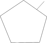
Figure 4. Regular pentagon with a hair.

An immediate consequence of Theorem 2 is that circumscriptible polygons as above (in particular, $n$-sided regular polygons) are spectrally determined in the class of convex polygons:

Corollary 7.

Let $P_{n}$ be a circumscriptible $n$-sided polygon whose angles are all equal but possibly one, which must then be larger than the rest. If a convex polygon $P$ has the same Dirichlet or Neumann spectrum as $P_{n}$, then it is congruent to it.

3. Reduction to a problem for polygons and conclusion of the proof

In view of Corollary 7, Theorem 1 will follows once we prove that a convex piecewise smooth domain (possible with straight corners) that is isospectral to a polygon must be a polygon too. This is an easy consequence of the fact that the fourth order term in the asymptotic expansion of the (Dirichlet or Neumann) heat trace is zero if and only if the boundary of the domain consists of segments:

Proposition 8.

Let $\Omega$ be a piecewise smooth domain with $m\geqslant 0$ straight corners. Then the asymptotic behavior of its Dirichlet heat trace at small times is

$$h_{\Omega}^{\mathrm{Dir}}(t)=\frac{|\Omega|}{4\pi t}-\frac{|\partial\Omega|}{8\sqrt{\pi t}}+\frac{1}{12\pi}\bigg{(}\int_{\partial\Omega}\kappa\,ds+\sum_{k=1}^{m}\frac{\pi^{2}-\theta_{k}^{2}}{2\theta_{k}}\bigg{)}+\frac{\sqrt{t}}{256\sqrt{\pi}}\int_{\partial\Omega}\kappa^{2}\,ds+O(t)\,,$$

where $\theta_{k}\in(0,2\pi)$ is the interior angle at the $j^{\text{th}}$ corner point, $\kappa$ is the curvature of the boundary at each differentiable point and $s$ is an arc-length parameter. Likewise, in the case of Neumann boundary conditions one has

$$h_{\Omega}^{\mathrm{Neu}}(t)=\frac{|\Omega|}{4\pi t}+\frac{|\partial\Omega|}{8\sqrt{\pi t}}+\frac{1}{12\pi}\bigg{(}\int_{\partial\Omega}\kappa\,ds+\sum_{k=1}^{m}\frac{\pi^{2}-\theta_{k}^{2}}{2\theta_{k}}\bigg{)}+\frac{5\sqrt{t}}{256\sqrt{\pi}}\int_{\partial\Omega}\kappa^{2}\,ds+O(t)\,.$$

Proof.

If the domain is smooth, the coefficients of the asymptotic expansion of the heat trace can be found in [3]. In the Dirichlet case, the contribution of a straight corner was first reported by Ray and a full proof can be found in [2]. In the Neumann case, the contribution of a straight corner can be found in [16]. As is customary, the sum of the coefficients of the smooth domain and of the straight corner gives the final formula presented in the statement. ∎

An immediate corollary of Proposition 8, which together with Corollary 7 completes the proof of Theorem 1, is the following:

Corollary 9.

A piecewise smooth domain with straight corners to a polygon must be a polygon.

Proof.

Since the term of order $\sqrt{t}$ in the asymptotic expansion of the heat trace of $\Omega$ must vanish, we infer that

$$\int_{\partial\Omega}\kappa^{2}\,ds=0\,,$$

i.e., that the boundary of $\Omega$ is flat. Hence it must consist of segments, so $\Omega$ is a polygon. ∎

References

• [1] M. Abramowitz, I.A. Stegun, Handbook of mathematical functions, Dover, New York, 1970.
• [2] M. van den Berg, S. Srisatkunarajah, Heat equation for a region in $\mathbb{R}^{2}$ with a polygonal boundary, J. London Math. Soc. 37 (1988) 119–127.
• [3] T.B. Branson, P.B. Gilkey, The asymptotics of the Laplacian on a manifold with boundary, Comm. PDE 15 (1990) 245–272.
• [4] J. Cheeger, Spectral geometry of singular Riemannian spaces, J. Differential Geometry 18 (1984) 575–657.
• [5] V. Cirtoaje, The equal variable method, J. Ineq. Pure Appl. Math. 8 (2007) 15(21).
• [6] C. Croke, V.A. Sharafutdinov, Spectral rigidity of a compact negatively curved manifold, Topology 37 (1998) 1265–1273.
• [7] C. Durso, Solution of the inverse spectral problem for triangles, Ph.D. thesis, Massachusetts Institute of Technology, 1990.
• [8] C. Gordon, D. Webb, S. Wolpert, Isospectral plane domains and surfaces via Riemannian orbifolds, Invent. Math. 110 (1992) 1–22.
• [9] D. Grieser and S. Maronna, Hearing the shape of a triangle, Notices Amer. Math. Soc. 60 (2013) 1440–1447.
• [10] V. Guillemin, D. Kazhdan, Some inverse spectral results for negatively curved 2-manifolds, Topology 19 (1980) 301–312.
• [11] H. Hezari, S. Zelditch, Inverse spectral problem for analytic $(\mathbb{Z}/2\mathbb{Z})^{n}$-symmetric domains in $\mathbb{R}^{n}$, Geom. Funct. Anal. 20 (2010) 160–191.
• [12] H. Hezari, Z. Lu, J. Rowlett, The Neumann isospectral problem for trapezoids, Annales Henri Poincaré, to appear.
• [13] M. Kac, Can one hear the shape of a drum? Amer. Math. Monthly 73 (1966) 1–23.
• [14] S. L’Huilier, De relatione mutua capacitatis et terminorum figurarum, geometrice considerata: seu de maximis et minimis, Michael Groöll, Warsaw, 1782. DOI:10.3931/e-rara-4049
• [15] Z. Lu, J.M. Rowlett, One can hear the corners of a drum, Bull. London Math. Soc. 48 (2016) 85–93.
• [16] R. Mazzeo, J. Rowlett, A heat trace anomaly on polygons, Math. Proc. Cambridge Philos. Soc. 159 (2015) 303–319.
• [17] B. Osgood, R. Phillips, P. Sarnak, Compact isospectral sets of surfaces, J. Funct. Anal. 80 (1988) 212–234.
• [18] B. Osgood, R. Phillips, P. Sarnak, Compact isospectral sets of plane domains, Proc. Nat. Acad. Sci. 85 (1988) 5359–5361.
• [19] B. Osgood, R. Phillips, P. Sarnak, Moduli space, heights and isospectral sets of plane domains, Ann. of Math. 129 (1989) 293–362.
• [20] G.P. Paternain, M. Salo, G. Uhlmann, Spectral rigidity and invariant distributions on Anosov surfaces, J. Differential Geom. 98 (2014) 147–181.
• [21] L. Smith, The asymptotics of the heat equation for a boundary value problem, Invent. Math. 63 (1981) 467–493.
• [22] J. Steiner, Sur le maximum et le minimum des figures dans le plan, sur la sphère, et dans l’espace en général, J. Math. Pures Appl. 6 (1841) 105–170.
• [23] Z.I. Szabo, Isospectral pairs of metrics on balls, spheres, and other manifolds with different local geometries, Ann. of Math. 154 (2001) 437–475.
• [24] S. Tanno, Eigenvalues of the Laplacian of Riemannian manifolds, Tohoku Math. J. 25 (1973) 391–403.
• [25] K. Watanabe, Plane domains which are spectrally determined II, J. Inequal. Appl. 7 (2002) 25–47.
• [26] S. Zelditch, Inverse spectral problem for analytic domains II. $\mathbb{Z}_{2}$-symmetric domains, Ann. of Math. 170 (2009) 205–269.