Abstract

We explore the idea of an alternative candidate for particle dark matter namely Feebly Interacting Massive Particle (FIMP) in the framework of a two component singlet scalar model. Singlet scalar dark matter has already been demonstrated to be a viable candidate for WIMP (Weakly Interacting Massive Particle) dark matter in literature. In the FIMP scenario, dark matter particles are slowly produced via “thermal frreze-in” mechanism in the early Universe and are never abundant enough to reach thermal equilibrium or to undergo pair annihilation inside the Universe’s plasma due to their extremely small couplings. We demonstrate that for smaller couplings too, required for freeze-in process, a two component scalar dark matter model considered here could well be a viable candidate for FIMP. In this scenario, the Standard Model of particle physics is extended by two gauge singlet real scalars whose stability is protected by an unbroken $Z_{2}\times{Z^{\prime}}_{2}$ symmetry and they are assumed to acquire no VEV after Spontaneous Symmetry Breaking. We explore the viable mass regions in the present two scalar DM model that is in accordance with the FIMP scenario. We also explore the upper limits of masses of the two components from the consideration of their self interactions.

1 Introduction

One of the most important problems of fundamental physics is to ascertain the particle nature of dark matter (DM) and their production mechanisms in the early Universe. The existence of dark matter in the Universe is established only through its gravitational effects and from different astronomical and cosmological observations such as rotation curves of spiral galaxies [1], gravitational lensing [2], phenomenon of Bullet cluster [3], PLANCK [4] satellite borne experiment for measuring the anisotropies in Cosmic Microwave Background Radiation (CMBR) etc. The direct evidence of dark matter through the direct detection mechanism [5]-[7] whereby a detector nucleus scatters off by a possible DM particle is yet to be found. One of the viable and popular candidates for dark matter may be the WIMPs (Weakly Interacting Massive Particles) [8]-[13]. But the particle candidates for WIMPs are not known yet. Also not known whether the dark matter in the Universe is made up of one particle component or its constituent components are more than one.

Although the WIMPs are yet to be detected in the world wide endeavour for direct dark matter search they continue to be popular dark matter candidates. WIMPs are produced in the early Universe thermally and they maintained thermal and chemical equilibrium at that epoch. When expansion rate of the Universe exceeded the interaction rates of the DM particles, these particles were not able to interact with them anymore. As a result such dark matter particles fell out of (or moved away from) equilibrium. Thus they suffered a state of “freeze out” by being decoupled from the Universe’s plasma and remained as relics. There are abundant examples in the literature where various particle physics models are proposed for viable particle candidates of WIMP dark matter. Such models are either based on simple extensions of Standard Model of particle physics (SM) or other established theories Beyond Standard Model (BSM). Some well-known candidates in the latter category are the neutralinos [8] in supersymmetric (SUSY) theories, the lightest Kaluza-Klein particle [14] in Universal Extra-Dimensional (UED) model, the singlet [15]-[18] etc. while the former category includes, among other models, the singlet and doublet [19]-[31] scalar extensions of the SM, singlet fermionic dark matter [32]-[34], hidden sector vector dark matter [35]-[38] etc. Vector and scalar dark matter in a model with scale invariant SM extended by a dark sector has been explored in [39, 40]. Fermion dark matter in a dark sector (with gauge group $\rm SU(2)\times\rm U(1)$) and dark $\rm U(1)$ charge are considered by Biswas et. al. [41]. But there is no definitive evidences that dark matter is in fact consists of WIMP particles [42] or other particles that are thermally produced in the early Universe. It is important therefore to consider viable alternatives to thermal WIMPs.

In this work we explore, for a viable dark matter candidate, a well motivated alternative to the WIMP mechanism, namely the FIMP (Feebly Interacting Massive Particle) [43, 44, 45, 46] mechanism. Here, we propose a dark matter candidate that has two components and the production of which in the early Universe are assumed to be through the FIMP mechanism. FIMPs are identified by their small interaction rates with Standard Model particles in the early Universe. Due to such feeble interactions these FIMP particles are unable to reach thermal equilibrium with the Universe’s plasma throughout their cosmological history. FIMPs are thus slowly produced by decays or annihilations of Standard Model particles in the thermal plasma and in contrast to WIMPs they are never abundant enough to undergo annihilation interactions among themselves. Therefore they are never in thermal or chemical equilibrium with rest of the Universe’s plasma. But their number densities increase slowly due to their very small couplings with the SM particles. Thus, in contrast to thermal WIMP cases where the dark matter particles go away from the equilibrium, the FIMP particles approach towards equilibrium. An example of a FIMP candidate may be sterile neutrino, which is produced from the decay of some heavy scalars [47]-[49] or gauge bosons [50]. In Refs. [51]-[53] various FIMP type DM candidates have been discussed.

In the present work we propose a two component dark matter model in FIMP scenario. The model involves two distinct singlet scalars that serve as the two components of the dark matter. Our purpose is to demonstrate the viablity of such two component singlet scalars in FIMP scenario to be dark matter candidates in the mass regimes spanning from GeV to keV. To this end, three pairs of masses are considered for the dark matter components in the mass regimes GeV, MeV and keV. For a one component singlet scalar dark matter model, the Standard Model is minimally extended by an additional scalar singlet [15]. In our work (involving two scalar components) we extend the scalar sector of SM by two real scalar fields $S_{2}$ and $S_{3}$, both of which are singlets under the Standard Model gauge group $\rm SU(2)_{L}\times\rm U(1)_{Y}$. Productions of both dark matter components in FIMP scenario proceed from the pair annihilation of SM particles such as fermions, gauge bosons and Higgs bosons. These scalars are assumed to acquire no vacuum expectations values (VEV) at spontaneous symmetry breaking (SSB) and a ${Z}_{2}\times{Z^{\prime}}_{2}$ symmetry [54, 55, 56] is imposed on the two scalars of the extended scalar sector so as to prevent the interactions of the two scalar components with the SM fermions or their decays. Here discrete symmetries $Z_{2}$ and ${Z^{\prime}}_{2}$ are imposed on the scalars $S_{2}$ and $S_{3}$ respectively. As both the scalars do not generate any VEV at SSB, the fermion masses are also not affected. Such a scalar interacts with the SM sector only through a Higgs portal due to the interaction term (in inteaction Lagrangian) of the type ${H}^{\dagger}HS_{i}S_{i}$ (where $i=2,3$). The unknown couplings of these additional scalars are the parameters of the theory. These can be constrained using the theoretical bounds on the Lagrangian as also by computing the relic densities and then comparing them with the same given by PLANCK experiment.

The relic densities are calculated by evaluating the comoving number densities $n_{s_{2}}$ and $n_{s_{3}}$ (which are in general written in terms of the ratios $Y_{s_{2}}=\frac{n_{S_{2}}}{S}$ and $Y_{s_{3}}=\frac{n_{s_{3}}}{S}$ of corresponding number densities and the entropy density $S$ of the Universe) for the scalar dark matter components $s_{2}$ and $s_{3}$ respectively (see later (Sect. 3)). At the present epoch these are computed by solving self consistently, the relevant coupled Boltzmann equations for the two components. As mentioned earlier, in FIMP scenario the number density of a species evolves towards its equilibrium value from almost negligible initial abundance. This means, initially $Y_{s_{2}}\approx 0\approx Y_{s_{3}}$. Evolution of these abundances requires computations of the quantities such as the decay processes $h\rightarrow s_{j}s_{j}$ ($j=2,3$), where $h$ denotes the SM Higgs, the pair annihilation processes $x\bar{x}\rightarrow s_{j}s_{j}$, where $x$ can be $W^{\pm},Z,f(\bar{f}),h,s_{2},s_{3}$ etc. The total dark matter relic density for the considered two component singlet scalar model in FIMP scenario is finally obtained by adding the computed individual abundances of each of the components as $\Omega_{\rm tot}{\tilde{h}}^{2}=\Omega_{s_{2}}{\tilde{h}}^{2}+\Omega_{s_{3}}{\tilde{h}}^{2}$, where the relic density $\Omega$ for a particular species is expressed in terms of $\Omega{\tilde{h}}^{2}$, ${\tilde{h}}$ being the Hubble parameter normalised to 100 km s^-1 Mpc^-1. The computed value of $\Omega_{\rm tot}{\tilde{h}}^{2}$ should be consistent with WMAP [57]/PLANCK [4] observational results, $0.1172\leq\Omega_{\rm DM}{\tilde{h}}^{2}\leq 0.1226$.

There are indications from astronomical observations of collisions of galaxies and galaxy clusters, the existence of self interactions among the dark matter paricles. From observations of Bullet Cluster phenomenon in the past and from more recent observations of 72 colliding galaxy clusters [58], an upper limit to the dark matter self interacting cross-sections per unit dark matter mass has been given in the literatures. In this work we explore further the mass regions for our two component FIMP dark matter model that agrees to this self interaction bound while satisfying other conditions mentioned earlier.

The paper is organised as follows. In Section 2 we give a brief account of the Freeze-in process. Section 3 furnishes our two component scalar dark matter model whicle Section 4 deals with the constraints by which the model parameter space can be constrained. In Section 5 the methodology to compute the relic densities for the present two component scalar DM model is described. In Section 6 we furnish our calculational results considering the dark matter candidates in three mass regions namely GeV, MeV and keV. As mentioned, we have also computed the dark matter self interactions for the present scenario. The formalism computations for the same are given in Section 7. Finally in Section 8 we give a brief summary and discussions.

2 Freeze-in Overview

In this section, we briefly discuss the “freeze-out” mechanism for thermal production of the dark matter. In the early Universe massive DM candidates could be thermally produced by the collision of the particles in thermal cosmic plasma and were in both kinetic and chemical equilibrium with the thermal plasma. Dark matter particles have a large initial thermal density at a temperature $T$ which is greater than the mass of DM ($m_{\chi}$, where $\chi$ denotes a thermal dark matter candidate). As the temperature of the hot plasma of the early Universe dropped below the mass of the dark matter, the lighter particles lacked the potential to produce heavier particles as they no more have enough kinetic energy (thermal energy). The expansion of the Universe dilutes the number of particles and thus interaction between them can hardly occur. Thus the conditions for thermal equilibrium were violated. The DM particles then go away from the equilibrium and decouple from Universal hot plasma. This phenomenon is called “freeze-out”. After “freeze-out” the comoving number density of DM particles became fixed and these particles remain as relic. Larger the annihilation cross-sections of the particles more is the annihilation of DM particles before freeze out and consequently the density will be less. An attractive feature of the freeze-out mechanism is that for renormalisable couplings the yield is dominated by low temperatures with freeze-out typically occuring at a temperature which is a factor $\sim 20-25$ of the DM mass. The WIMPs are generally produced through this mechanism.

As mentioned in Section 1, we explore in this paper, a dark matter candidate that is produced through an alternate mechanism namely the “freeze-in” mechanism from almost negligible initial abundance and with very feeble interactions with other particles. The dark matter produced through this mechanism is generally referred to as Feebly Interacting Massive Particles (FIMPs) dark matter. As the interaction of such FIMPs with other bath particles (Standard Model particles) are very feeble, they never attain thermal equilibrium. Although feeble, initially the FIMPs production may happen slowly due to the very feeble interactions with the Standard Model particles which grow gradually. The dominant production occurs at $T\sim m_{\chi}$, where $T$ is the temperature of the Universe.

The freeze-in process is opposite in nature to that of freeze-out. As the temperature $T$ drops below the mass of the relevant particle (here the DM candidate), the DM is either heading away from (freeze-out) or towards (freeze-in) thermal equilibrium. In freeze-out mechanism the initial number density varies as $T^{3}$ and then decreases as the interaction strength reduces to maintain this large abundance. On the other hand freeze-in has a negligible initial DM abundance, and increases as the interaction strength increases the production of DM from the thermal bath.

3 Two Component Dark Matter Model

The two component dark matter model in FIMP scenario proposed in this work consists of two distinct scalar singlet DM particles $S_{2}$ and $S_{3}$. Here, we have a renormalisable extension of the SM by adding two real scalar fields $S_{2}$ and $S_{3}$. These two real scalars are singlets under the SM gauge group and they are stabilised by imposing a discrete $Z_{2}\times Z_{2}^{\prime}$ symmetry. These scalars do not generate any VEV after spontaneous symmetry breaking and there is no mixing between these real scalars and the SM scalar. The only possible way that the DM candidates interact with the SM sector is through Higgs portal.

The Lagrangian of our model can be written as

$${\cal L}={\cal L}_{\rm SM}+{\cal L}_{\rm DM}+{\cal L}_{\rm int}\,\,,$$ (1)

where $\mathcal{L}_{\rm SM}$ stands for the Lagrangian of the SM particles and it consists of quadratic and quartic terms involving the Higgs doublet $H$ in addition to the usual kinetic term for $H$. As mentioned, the dark sector Lagrangian consists of two real scalar fields, which can be expressed as

$${\cal L}_{\rm DM}={\cal L}_{S_{2}}+{\cal L}_{S_{3}}\,\,,$$ (2)

with

$${\cal L}_{S_{2}}=\frac{1}{2}(\partial_{\mu}S_{2})(\partial^{\mu}S_{2})-\frac{{\mu}_{S_{2}}^{2}}{2}S_{2}^{2}-\frac{\lambda_{S_{2}}}{4}S_{2}^{4}\,\,,$$ (3)

and

$${\cal L}_{S_{3}}=\frac{1}{2}(\partial_{\mu}S_{3})(\partial^{\mu}S_{3})-\frac{{\mu}_{S_{3}}^{2}}{2}S_{3}^{2}-\frac{\lambda_{S_{3}}}{4}S_{3}^{4}\,\,.$$ (4)

The interaction Lagrangian $\mathcal{L}_{\rm int}$ contains all possible mutual interaction terms among the scalar fields $H,S_{2},S_{3}$.

$${\cal L}_{\rm int}=-V^{\prime}(H,S_{2},S_{3})\,\,,$$ (5)

where $V^{\prime}(H,S_{2},S_{3})$ can be written as

$$V^{\prime}(H,\,S_{2},\,S_{3})={\lambda_{HS_{2}}}H^{\dagger}H\,S_{2}^{2}+{\lambda_{HS_{3}}}H^{\dagger}H\,S_{3}^{2}+\lambda_{S_{2}S_{3}}S_{2}^{2}\,S_{3}^{2}\,\,.$$ (6)

The renormalisable scalar potential $V$ is written as

$$V = \mu_{H}^{2}\,H^{\dagger}H+\lambda_{H}\,(H^{\dagger}H)^{2}+\frac{\mu_{S_{2}}^{2}}{2}S_{2}^{2}+\frac{\lambda_{S_{2}}}{4}S_{2}^{4}+\frac{{\mu}_{S_{3}}^{2}}{2}S_{3}^{2}+\frac{\lambda_{S_{3}}}{4}S_{3}^{4}$$ (7)

$$+{\lambda_{HS_{2}}}H^{\dagger}H\,S_{2}^{2}+{\lambda_{HS_{3}}}H^{\dagger}H\,S_{3}^{2}+\lambda_{S_{2}S_{3}}S_{2}^{2}\,S_{3}^{2}\,.$$

After the spontaneous symmetry breaking SM Higgs acquires a VEV, $v$ ($v$ $\sim$ 246 GeV) and SM scalar doublet takes the form

$$H=\frac{1}{\sqrt{2}}\left(\begin{array}[]{c}0\\ v+h\end{array}\right)\,\,.$$ (10)

It is assumed in the present model that the two scalars $S_{2}$ and $S_{3}$ do not generate any VEV such that $\langle S_{2}\rangle=0=\langle S_{3}\rangle$. As a result, after SSB we have $H\rightarrow h+v$, $S_{2}=s_{2}+0,S_{3}=s_{3}+0$. Thus after spontaneous symmetry breaking the scalar potential $V$ takes the form

$$V = \frac{\mu_{H}^{2}}{2}(v+h)^{2}+\frac{\lambda_{H}}{4}(v+h)^{4}+\frac{\mu_{S_{2}}^{2}}{2}s_{2}^{2}+$$ (11)

$$\frac{\lambda_{S_{2}}}{4}s_{2}^{4}+\frac{\mu_{S_{3}}}{2}s_{3}^{2}+\frac{\lambda_{S_{3}}}{4}s_{3}^{4}+$$

$$\frac{\lambda_{HS_{2}}}{2}(v+h)^{2}s_{2}^{2}+\frac{\lambda_{HS_{3}}}{2}(v+h)^{2}s_{3}^{2}+\lambda_{S_{2}S_{3}}s_{2}^{2}s_{3}^{2}\,\,.$$

Now by using the minimisation condition

$$\left(\frac{\partial V}{\partial h}\right),\,\left(\frac{\partial V}{\partial s_{2}}\right),\,\left(\frac{\partial V}{\partial s_{3}}\right)\Bigg{|}_{h=0,\,s_{2}=0,\,s_{3}=0}=0\,\,,$$ (12)

we obtain the condition

$$\mu_{H}^{2}+\lambda_{H}v^{2}=0\,\,.$$ (13)

By evaluating $\frac{\partial^{2}V}{\partial h^{2}}$, $\frac{\partial^{2}V}{\partial s_{2}^{2}}$, $\frac{\partial^{2}V}{\partial s_{3}^{2}}$, $\frac{\partial^{2}V}{{\partial h}{\partial s_{2}}}$, $\frac{\partial^{2}V}{{\partial h}{\partial s_{3}}}$, $\frac{\partial^{2}V}{{\partial s_{3}}{\partial s_{2}}}$ at $h=s_{2}=s_{3}=0$, one can now construct the mass matrix in the basis $h-s_{2}-s_{3}$ as

$$\mathcal{M}^{2}_{\rm scalar} = \left(\begin{array}[]{ccc}2\lambda_{H}v^{2}&0&0\\ 0&\mu_{S_{2}}^{2}+\lambda_{HS_{2}}v^{2}&0\\ 0&0&\mu_{S_{3}}^{2}+\lambda_{HS_{3}}v^{2}\end{array}\right).$$ (17)

It may be noted here that the mass matrix is diagonal as there is no mixing between $h$, $s_{2}$ and $s_{3}$.

4 Constraints

In this section we discuss various bounds and constraints on the model parameters of the model from both theoretical considerations and experimental observations. These are furnished in the following. $\bullet$ Vacuum Stability: In our work we consider an extended model with two additional scalar fields. For the stability of the vacuum, the scalar potential has to be bounded from below in the limit of large field values along all possible directions of the field space. In this large limit the quartic terms of the scalar potential dominate over the mass and the cubic terms. The quartic part ($V_{4}$) of the scalar potential $V$ (Eq. (7)) is given as

$$V_{4} = \lambda_{H}\,(H^{\dagger}H)^{2}+\frac{\lambda_{S_{2}}}{4}S_{2}^{4}+\frac{\lambda_{S_{3}}}{4}S_{3}^{4}+{\lambda_{HS_{2}}}H^{\dagger}H\,S_{2}^{2}$$ (18)

$$+{\lambda_{HS_{3}}}H^{\dagger}H\,S_{3}^{2}+\lambda_{S_{2}S_{3}}S_{2}^{2}\,S_{3}^{2}\,.$$

Bounds on the couplings from the vacuum stability condition are [59]

$$\lambda_{H},\,\,\lambda_{S_{2}},\,\,\lambda_{S_{3}} > 0$$

$$\lambda_{HS_{2}}+\sqrt{\lambda_{H}\lambda_{S_{2}}} > 0$$

$$\lambda_{HS_{3}}+\sqrt{\lambda_{H}\lambda_{S_{3}}} > 0$$

$$2\lambda_{S_{2}S_{3}}+\sqrt{\lambda_{S_{2}}\lambda_{S_{3}}} > 0$$ (19)

and

$$\sqrt{2(\lambda_{HS_{2}}+\sqrt{\lambda_{H}\lambda_{S_{2}}})(\lambda_{HS_{3}}+\sqrt{\lambda_{H}\lambda_{S_{3}}})(2\lambda_{S_{2}S_{3}}+\sqrt{\lambda_{S_{2}}\lambda_{S_{3}}})}$$

$$+\sqrt{\lambda_{H}\lambda_{S_{2}}\lambda_{S_{3}}}+\lambda_{HS_{2}}\sqrt{\lambda_{S_{3}}}+\lambda_{HS_{3}}\sqrt{\lambda_{S_{2}}}+2\lambda_{S_{2}S_{3}}\sqrt{\lambda_{H}}>0\,\,.$$ (20)

$\bullet$ Perturbativity: In order to obey the perturbative limit, the quartic couplings of the scalar potential in our model should be constrained as [54]-[60]

$$\lambda_{H},\,\,\lambda_{HS_{2}},\,\,\lambda_{HS_{3}}\leq 4\pi,$$

$$\lambda_{S_{2}},\,\,\lambda_{S_{3}},\,\,\lambda_{S_{2}S_{3}}\leq\displaystyle\frac{2\pi}{3}.$$ (21)

$\bullet$ Relic Density: The total relic density of the dark matter components must satisfy PLANCK observational results for dark matter relic densities.

$$0.1172\leq\Omega_{\rm DM}{\tilde{h}}^{2}\leq 0.1226\,\,,$$ (22)

where $\Omega_{\rm DM}$ is the dark matter relic density normalised to the critical density of the Universe and ${\tilde{h}}$ is the Hubble parameter in units of 100 Km s^-1 Mpc^-1. $\bullet$ Collider Physics Bounds: ATLAS and CMS had observed independently the excess in $\gamma\gamma$ channel from which they had confirmed the existence of a Higgs like scalar with mass $\sim$ 125.5 GeV [61, 62]. The signal strength of Higgs like boson is defined as

$$R = \displaystyle\frac{\sigma(pp\rightarrow h)}{\sigma^{\rm{SM}}(pp\rightarrow h)}\displaystyle\frac{{\rm{Br}}(h\rightarrow xx)}{{\rm{Br}}^{\rm{SM}}(h\rightarrow xx)}\,\,\,,$$ (23)

where $\sigma(pp\rightarrow h)$ and ${\rm Br}(h\rightarrow xx)$ denote the production cross-section and the decay branching ratio of Higgs like particle decaying into SM particles ($x$) respectively while $\sigma^{\rm SM}(pp\rightarrow h)$ and ${\rm Br}^{\rm SM}(h\rightarrow xx)$ respectively are those for SM Higgs. The braching ratio of Higgs like boson and SM Higgs boson can be expressed respectively as ${\rm Br}(h\rightarrow xx)=\displaystyle\frac{\Gamma(h\rightarrow xx)}{\Gamma}$ and ${\rm Br}^{\rm SM}(h\rightarrow xx)=\displaystyle\frac{\Gamma^{\rm SM}(h\rightarrow xx)}{\Gamma^{\rm SM}}$, where $\Gamma(h\rightarrow xx)$ and $\Gamma^{\rm SM}(h\rightarrow xx)$ are the decay width of Higgs like boson and SM Higgs boson. The quantities $\Gamma$ and $\Gamma^{\rm SM}$ represent the total decay widths of Higgs like particle and SM Higgs boson respectively. Using these expressions for branching ratio in Eq. (23) one obtains

$$R=\displaystyle\frac{\sigma(pp\rightarrow h)}{\sigma^{\rm SM}(pp\rightarrow h)}\displaystyle\frac{\Gamma(h\rightarrow xx)}{\Gamma}\displaystyle\frac{\Gamma^{\rm SM}}{\Gamma^{\rm SM}(h\rightarrow xx)}\,\,.$$ (24)

As there is no mixing between the scalars ($h$, $s_{2}$ and $s_{3}$) we have $\sigma(pp\rightarrow h)\equiv\sigma^{\rm SM}(pp\rightarrow h)$ and similarly $\Gamma(h\rightarrow xx)\equiv\Gamma^{\rm SM}(h\rightarrow xx)$. Thus Eq. (24) takes the form

$$R=\displaystyle\frac{\Gamma^{\rm SM}}{\Gamma}\,\,.$$ (25)

In the above expressions the total decay width of Higgs like boson can be wriiten as $\Gamma=\Gamma^{\rm SM}+\Gamma^{\rm inv}$. The invisible decay width of Higgs like boson to dark matter particles $\Gamma^{\rm inv}$ is given as

$$\Gamma^{\rm inv}=\Gamma_{h\rightarrow s_{2}s_{2}}+\Gamma_{h\rightarrow s_{3}s_{3}}\,\,.$$ (26)

The decay width $\Gamma_{h\rightarrow s_{i}s_{i}}$ ($i=2,3$) can be expressed as

$$\Gamma_{h\rightarrow s_{i}s_{i}}=\displaystyle\frac{\lambda_{hs_{i}s_{i}}}{8\pi m_{h}}\sqrt{1-\displaystyle\frac{4m^{2}_{s_{i}}}{m_{h}^{2}}}\,\,.$$ (27)

The invisible branching ratio for such invisible decay is then given as

$${\rm Br}^{\rm inv}=\displaystyle\frac{\Gamma^{\rm inv}(h\rightarrow s_{i}s_{i})}{\Gamma_{h}},i=2,3\,\,.$$ (28)

We have checked that due to the small values of the couplings in our model this branching ratio (Eq. (28)) for the invisible decay of Higgs like boson has to be small. To this end, we impose the condition ${\rm Br}^{\rm inv}<0.2$ [63] and that the Higgs like boson signal strength must satisfy the limit $R\geq 0.8$ [64].

5 Relic Density Calculations for Two Component Scalar FIMP Dark Matter

The evolution of the number density of DM particle with time is governed by the Boltzmann equation. In this section we compute the number densities for both the DM candidates $s_{2}$ and $s_{3}$ in our model, at the present epoch (temperature $T_{0}$ $\sim$ $10^{-13}$ GeV). For the case of a two component dark matter, the relic density is obtained by solving self consistently, two coupled Boltzmann equations which, for the present scenario, are given by

$$\displaystyle\frac{dn_{s_{2}}}{dt}+3{\tilde{H}}n_{s_{2}} = -{\langle\Gamma_{h\rightarrow s_{2}s_{2}}\rangle}(n_{s_{2}}-n_{s_{2}}^{\rm eq})-{\langle\sigma v\rangle}_{s_{2}s_{2}\rightarrow x\bar{x}}(n_{s_{2}}^{2}-(n_{s_{2}}^{\rm eq})^{2})$$ (29)

$$-{\langle\sigma v\rangle}_{s_{2}s_{2}\rightarrow s_{3}s_{3}}\left(n_{s_{2}}^{2}-\displaystyle\frac{(n_{s_{2}}^{\rm eq})^{2}}{(n_{s_{3}}^{\rm eq})^{2}}n_{s_{3}}^{2}\right)\,\,,$$

$$\displaystyle\frac{dn_{s_{3}}}{dt}+3{\tilde{H}}n_{s_{3}} = -{\langle\Gamma_{h\rightarrow s_{3}s_{3}}\rangle}(n_{s_{3}}-n_{s_{3}}^{\rm eq})-{\langle\sigma v\rangle}_{s_{3}s_{3}\rightarrow x\bar{x}}(n_{s_{3}}^{2}-(n_{s_{3}}^{\rm eq})^{2})$$ (30)

$$+{\langle\sigma v\rangle}_{s_{2}s_{2}\rightarrow s_{3}s_{3}}\left(n_{s_{2}}^{2}-\displaystyle\frac{(n_{s_{2}}^{\rm eq})^{2}}{(n_{s_{3}}^{\rm eq})^{2}}n_{s_{3}}^{2}\right)\,\,.$$

In the above, $n_{s_{i}}$ and $n^{\rm eq}_{s_{i}}$ ($i=2,3$) are the number densities (that evolve with time $t$) and equilibrium number densities respectively for the scalars $s_{2}$ and $s_{3}$, $\langle\sigma v\rangle_{s_{i}s_{i}}\rightarrow ab$ denotes the average annihilation cross-sections for the two scalars $s_{i},i=2,3$ ($a$, $b$ are the annihilation products) and ${\tilde{H}}$ is the Hubble parameter.

This is to mention that the Boltzmann equations (Eqs. (29, 30) ) should also in principle include terms due to $4\rightarrow 2$ or $3\rightarrow 2$ interactions of the dark matter self annihilations. The annihilation cross-sections for such processes such as $s_{2}s_{2}s_{2}s_{2}\rightarrow s_{2}s_{2},s_{2}s_{2}s_{3}s_{3}\rightarrow s_{2}s_{3},s_{2}s_{2}s_{2}\rightarrow s_{2}s_{2},s_{2}s_{2}s_{3}\rightarrow s_{2}s_{3}$ could be significant if the couplings are large. For our cases we consider FIMP dark matter masses in three ranges namely keV, MeV and GeV while for GeV range such contributions are ruled out since for a significant contribution, the coupling is to be large enough that may violate perturbative limit [65]. In case of keV range we have checked (also by Ref. [66]) that $4\rightarrow 2$ interaction is insignificant due to smalleness of corresponding self coupling while for MeV range FIMP these could be significant. We have checked that for the chosen mass and the values of the couplings (obtained from theoretical constraints) the contribution is negligibly small even for MeV mass range FIMPs. From Fig. 3 of Ref. [67], we see that for the present work the contribution for MeV mass range falls in the semirelativistic region of the plot. Hence we did not consider these terms in the Boltzmann equations.

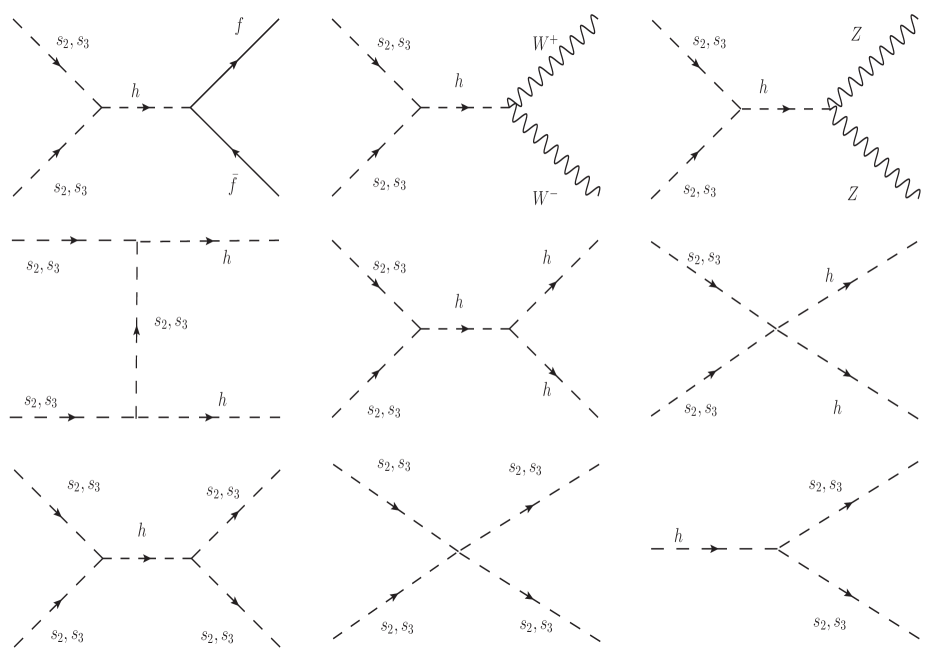
Figure 1: Feynman diagrams for both the scalar dark matter candidates $s_{2}$ and $s_{3}$.

Defining a dimensionless quantity namely the comoving number density expressed in terms of the ratio $Y_{i}=n_{s_{i}}/S$ ($i=2,3$) of the number density ($n_{s_{i}}$) and the total entropy density ($S$) and defining $z=m_{h}/T$, $T$ being the photon temperature, Eqs. (29, 30) can be rewritten in terms of the variation of $Y_{i}(i=2,3)$ with $z$ as

$$\displaystyle\frac{dY_{s_{2}}}{dz} = -\displaystyle\frac{2zm_{\rm Pl}}{1.66m_{h}^{2}}\displaystyle\frac{\sqrt{g_{*}(T)}}{\sqrt{g_{S}(T)}}\Bigg{(}\langle\Gamma_{h\rightarrow s_{2}s_{2}}\rangle\left(Y_{s_{2}}-Y_{h}^{\rm eq}\right)\Bigg{)}$$ (31)

$$-\displaystyle\frac{4\pi^{2}}{45}\displaystyle\frac{m_{\rm Pl}m_{h}}{1.66}\displaystyle\frac{\sqrt{g_{*}(T)}}{z^{2}}\times$$

$$\Bigg{(}\sum_{x=W,Z,f,h}\langle{\sigma v}_{x\bar{x}\rightarrow s_{2}s_{2}}\rangle(Y_{s_{2}}^{2}-({Y_{x}^{\rm eq}})^{2})+\langle{\sigma v}_{s_{2}s_{2}\rightarrow s_{3}s_{3}}\rangle(Y_{s_{2}}^{2}-\displaystyle\frac{(Y_{s_{2}}^{\rm eq})^{2}}{(Y_{s_{3}}^{\rm eq})^{2}}Y_{s_{3}}^{2})$$

$$-\langle{\sigma v}_{s_{3}s_{3}\rightarrow s_{2}s_{2}}\rangle(Y_{s_{3}}^{2}-\displaystyle\frac{(Y_{s_{3}}^{\rm eq})^{2}}{(Y_{s_{2}}^{\rm eq})^{2}}Y_{s_{2}}^{2})\Bigg{)}$$

and

$$\displaystyle\frac{dY_{s_{3}}}{dz} = -\displaystyle\frac{2zm_{\rm Pl}}{1.66m_{h}^{2}}\displaystyle\frac{\sqrt{g_{*}(T)}}{\sqrt{g_{S}(T)}}\Bigg{(}\langle\Gamma_{h\rightarrow s_{3}s_{3}}\rangle\left(Y_{s_{3}}-Y_{h}^{\rm eq}\right)\Bigg{)}$$ (32)

$$-\displaystyle\frac{4\pi^{2}}{45}\displaystyle\frac{m_{\rm Pl}m_{h}}{1.66}\displaystyle\frac{\sqrt{g_{*}(T)}}{z^{2}}\times$$

$$\Bigg{(}\sum_{x=W,Z,f,h}\langle{\sigma v}_{x\bar{x}\rightarrow s_{3}s_{3}}\rangle(Y_{s_{3}}^{2}-({Y_{x}^{\rm eq}})^{2})-\langle{\sigma v}_{s_{2}s_{2}\rightarrow s_{3}s_{3}}\rangle(Y_{s_{2}}^{2}-\displaystyle\frac{(Y_{s_{2}}^{\rm eq})^{2}}{(Y_{s_{3}}^{\rm eq})^{2}}Y_{s_{3}}^{2})$$

$$+\langle{\sigma v}_{s_{3}s_{3}\rightarrow s_{2}s_{2}}\rangle(Y_{s_{3}}^{2}-\displaystyle\frac{(Y_{s_{3}}^{\rm eq})^{2}}{(Y_{s_{2}}^{\rm eq})^{2}}Y_{s_{2}}^{2})\Bigg{)}\,\,.$$

We have already mentioned that the initial abundance of FIMP [43, 44] dark matter candidate is negligible. Therefore assuming $Y_{s_{2}}=Y_{s_{3}}=0$, Eqs. (31, 32) take the form

$$\displaystyle\frac{dY_{s_{2}}}{dz} = -\displaystyle\frac{2zm_{\rm Pl}}{1.66m_{h}^{2}}\displaystyle\frac{\sqrt{g_{*}(T)}}{\sqrt{g_{S}(T)}}\Bigg{(}\langle\Gamma_{h\rightarrow s_{2}s_{2}}\rangle\left(-Y_{h}^{\rm eq}\right)\Bigg{)}$$ (33)

$$-\displaystyle\frac{4\pi^{2}}{45}\displaystyle\frac{m_{\rm Pl}m_{h}}{1.66}\displaystyle\frac{\sqrt{g_{*}(T)}}{z^{2}}\times$$

$$\Bigg{(}\sum_{x=W,Z,f,h}\langle{\sigma v}_{x\bar{x}\rightarrow s_{2}s_{2}}\rangle(-{Y_{x}^{\rm eq}})^{2}\Bigg{)}$$

and

$$\displaystyle\frac{dY_{s_{3}}}{dz} = -\displaystyle\frac{2zm_{\rm Pl}}{1.66m_{h}^{2}}\displaystyle\frac{\sqrt{g_{*}(T)}}{\sqrt{g_{S}(T)}}\Bigg{(}\langle\Gamma_{h\rightarrow s_{3}s_{3}}\rangle\left(-Y_{h}^{\rm eq}\right)\Bigg{)}$$ (34)

$$-\displaystyle\frac{4\pi^{2}}{45}\displaystyle\frac{m_{\rm Pl}m_{h}}{1.66}\displaystyle\frac{\sqrt{g_{*}(T)}}{z^{2}}\times$$

$$\Bigg{(}\sum_{x=W,Z,f,h}\langle{\sigma v}_{x\bar{x}\rightarrow s_{3}s_{3}}\rangle(-{Y_{x}^{\rm eq}})^{2}\Bigg{)}\,\,.$$

In the above, $m_{\rm Pl}$ is the PLANCK mass, $m_{\rm Pl}$ = 1.22 $\times 10^{22}$ GeV and the term $g_{*}$ is defined as [12]

$$\sqrt{g_{*}(T)}=\displaystyle\frac{g_{S}(T)}{\sqrt{g_{\rho}{T}}}\Bigg{(}1+\displaystyle\frac{1}{3}\displaystyle\frac{dlnh_{\rm eff}(T)}{dlnT}\Bigg{)}\,\,,$$ (35)

where two effective degrees of freedom $g_{\rm eff}(T)$ and $h_{\rm eff}(T)$ are related to the energy and entropy densities of the Universe through the following relations,

$$S=g_{S}(T)\displaystyle\frac{2\pi^{2}}{45}T^{3}\,, \rho=g_{\rho}(T)\displaystyle\frac{\pi^{2}}{30}T^{4}\,\,.$$ (36)

Also, the thermally averaged decay widths and annihilation cross-sections for various processes are given by,

$$\langle\Gamma_{h\rightarrow s_{i}s_{i}}\rangle = \Gamma_{h\rightarrow s_{i}s_{i}}\frac{K_{1}(z)}{K_{2}(z)}\,\,,$$

$$\langle\sigma{\rm v}\rangle_{x\bar{x}\rightarrow s_{i}s_{i}} = \frac{1}{8m_{x}^{4}\,T\,K_{2}^{2}(M_{x}/T)}\int_{4m_{x}^{2}}^{\infty}\sigma_{x\bar{x}\rightarrow s_{i}s_{i}}(s-4M_{x}^{2})\sqrt{s}K_{1}(\displaystyle\frac{\sqrt{s}}{T})ds\,\,.$$ (37)

In Eq. (37) $i=2,3,x=W^{\pm},Z,f,h,s_{2},s_{3}$, $K_{1}$ and $K_{2}$ are the modified Bessel functions of order 1 and 2, $s$ defines the centre of momentum energy. The decay widths $\Gamma_{h\rightarrow S_{i}S_{i}}$ and annihilation cross-sections $\sigma_{x\bar{x}\rightarrow s_{i}s_{i}}$ ($i=2,3$) for different processes considered to calcuate the coupled Boltzmann equations (Eqs. (33, 34)) are given below

$$\Gamma_{h\rightarrow s_{i}s_{i}} = \displaystyle\frac{g^{2}_{hs_{i}s_{i}}}{8\pi m_{h}}\sqrt{1-\displaystyle\frac{4m^{2}_{s_{i}}}{m^{2}_{h}}}\,\,,$$ (38)

$$\sigma_{hh\rightarrow s_{i}s_{i}} = \displaystyle\frac{1}{2\pi s}\sqrt{\displaystyle\frac{s-4m^{2}_{s_{i}}}{s-4m^{2}_{h}}}\left\{g^{2}_{hhs_{i}s_{i}}+\displaystyle\frac{9\,\,g^{2}_{hhh}g^{2}_{hs_{i}s_{i}}}{[(s-m^{2}_{h})^{2}+(\Gamma_{h}m_{h})^{2}]}\right.$$ (39)

$$\left.-\displaystyle\frac{6\,\,g_{hhs_{i}s_{i}}g_{hs_{i}s_{i}}g_{hhh}(s-m^{2}_{h})}{[(s-m^{2}_{h})^{2}+(\Gamma_{h}m_{h})^{2}]}\right\}\,\,,$$

$$\sigma_{s_{2}s_{2}\rightarrow s_{3}s_{3}} = \displaystyle\frac{1}{2\pi s}\sqrt{\displaystyle\frac{s-4m^{2}_{s_{3}}}{s-4m^{2}_{s_{2}}}}\left\{g^{2}_{s_{2}s_{2}s_{3}s_{3}}+\displaystyle\frac{g^{2}_{s_{2}s_{2}h}g^{2}_{hs_{3}s_{3}}}{[(s-m^{2}_{h})^{2}+(\Gamma_{h}m_{h})^{2}]}\right.$$ (40)

$$\left.-\displaystyle\frac{2\,\,g_{s_{2}s_{2}s_{3}s_{3}}g_{s_{2}s_{2}h}g_{hs_{3}s_{3}}(s-m^{2}_{h})}{[(s-m^{2}_{h})^{2}+(\Gamma_{h}m_{h})^{2}]}\right\}\,\,,$$

$$\sigma_{s_{3}s_{3}\rightarrow s_{2}s_{2}} = \displaystyle\frac{1}{2\pi s}\sqrt{\displaystyle\frac{s-4m^{2}_{s_{2}}}{s-4m^{2}_{s_{3}}}}\left\{g^{2}_{s_{2}s_{2}s_{3}s_{3}}+\displaystyle\frac{g^{2}_{s_{3}s_{3}h}g^{2}_{hs_{2}s_{2}}}{[(s-m^{2}_{h})^{2}+(\Gamma_{h}m_{h})^{2}]}\right.$$ (41)

$$\left.-\displaystyle\frac{2g_{s_{3}s_{3}s_{2}s_{2}}g_{s_{3}s_{3}h}g_{hs_{2}s_{2}}(s-m^{2}_{h})}{[(s-m^{2}_{h})^{2}+(\Gamma_{h}m_{h})^{2}]}\right\}\,\,,$$

$$\sigma_{WW\rightarrow s_{i}s_{i}} = \displaystyle\frac{g^{2}_{WWh}g^{2}_{hs_{i}s_{i}}}{72\pi s}\sqrt{\displaystyle\frac{s-4m^{2}_{s_{i}}}{s-4m^{2}_{W}}}\displaystyle\frac{\left(3-\displaystyle\frac{s}{m^{2}_{W}}+\displaystyle\frac{s^{2}}{4m^{2}_{W}}\right)}{(s-m^{2}_{h})^{2}+(\Gamma_{h}m_{h})^{2}}\,\,,$$ (42)

$$\sigma_{ZZ\rightarrow s_{i}s_{i}} = \displaystyle\frac{g^{2}_{ZZh}g^{2}_{hs_{i}s_{i}}}{18\pi s}\sqrt{\displaystyle\frac{s-4m^{2}_{s_{i}}}{s-4m^{2}_{Z}}}\displaystyle\frac{\left(3-\displaystyle\frac{s}{m^{2}_{Z}}+\displaystyle\frac{s^{2}}{4m^{2}_{Z}}\right)}{(s-m^{2}_{h})^{2}+(\Gamma_{h}m_{h})^{2}}\,\,,$$ (43)

$$\sigma_{f\bar{f}\rightarrow s_{i}s_{i}} = \displaystyle\frac{N_{c}g^{2}_{ffh}g^{2}_{hs_{i}s_{i}}}{16\pi s}\displaystyle\frac{\sqrt{(s-4m^{2}_{s_{i}})(s-4m^{2}_{f})}}{(s-m^{2}_{h})^{2}+(\Gamma_{h}m_{h})^{2}}\,\,.$$ (44)

In the above equations the couplings of the vertices are defined as $g_{abc}$ and $g_{abcd}$, where $a,b,c,d$ are the fields. The masses of $W$ and $Z$ bosons and the fermions ($f$) are denoted as $m_{W}$, $m_{Z}$ and $m_{f}$ respectively. $N_{c}$ in Eq. (44) denotes the color quantum number. Detailed expressions for all the couplings required given in Eqs. (33 - 39) are enlisted in the Appendix. The Feynman diagrams corresponding to all the possible channels for the two distinct scalar components $s_{2}$ and $s_{3}$ are shown in Fig. 1.

The relic densities of each of the components $s_{2}$ and $s_{3}$ of the dark matter are finally obtained in terms of their respective masses and comoving number densities at the present epoch, as [68, 69]

$$\Omega_{i}{\tilde{h}}^{2}=2.755\times 10^{8}\left(\frac{m_{i}}{\rm GeV}\right)Y_{i}(T_{0}),\hskip 10.0pti=s_{2},s_{3}\,\,.$$ (45)

Solving numerically the two coupled Boltzmann equations Eqs. (31 - 34) alongwith Eqs. (33 - 39) we compute the comoving number densities $Y_{i}(T_{0})$ for both components of FIMP dark matter. The total relic density $\Omega_{\rm{tot}}$ is then obtained by adding the relic densities of each of the components $s_{2}$ and $s_{3}$ as follows

$$\Omega_{\rm tot}{\tilde{h}}^{2}=\Omega_{s_{2}}{\tilde{h}}^{2}+\Omega_{s_{3}}{\tilde{h}}^{2}\,\,.$$ (46)

The total relic density $\Omega_{\rm tot}{\tilde{h}}^{2}$ should satisfy the PLANCK measurement

$$\hskip 10.0pt0.1172\leq\Omega_{\rm DM}{\tilde{h}}^{2}\leq 0.1226\,\,.$$ (47)

As mentioned earlier, in our present dark matter model we have considered two distinct scalar dark matter particles in the FIMP scenario. In Fig. 2 we furnish representative plots showing the evolutions of relic densities for each of the components as well as the total relic densities of two component scalar dark matter for each of the chosen mass regimes namely GeV (Fig. 2a), MeV (Fig. 2b) and keV (Fig. 2c).

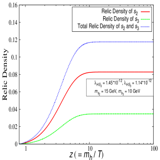
(a)

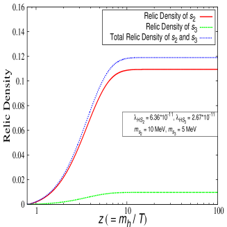
(b)

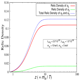
Figure 2: Variations of the relic densities of the two single scalar dark matter components $s_{2}$ and $s_{3}$ with $z$ for different values of couplings ($\lambda_{HS_{2}},\lambda_{HS_{3}}$) and masses ($m_{s_{2}},m_{s_{3}}$) in the three mass regions GeV (a), MeV (b) and keV (c) . In each plot (from (a) to (c)) the red solid line and the green dashed line indicate the relic density of the components $s_{2}$ and $s_{3}$ respectively while the blue dotted line represents the same for the total relic density. The PLANCK observational range for DM relic density is $0.1172\leq\Omega_{\rm DM}{\tilde{h}}^{2}\leq 0.1226$.

6 Calculations and Results

We have considered here a two component scalar dark matter model under the framework of Feebly Interacting Massive Particle (FIMP) dark matter. In this work this is our purpose to demonstrate that over a wide range of masses (from GeV to keV) such a two component FIMP scalar dark matter is a viable dark matter candidate. Therefore in our analysis we have chosen the DM candidates in three mass regimes namely GeV, MeV and keV. To this end we first calculate the relic densities of the FIMP dark matter candidates in our proposed model. From Section 3 it should be clear that the various unknown couplings ($\lambda_{HS_{2}},\lambda_{HS_{3}},\lambda_{S_{2}S_{3}}$ etc.) constitute the parameters of our model. We first constrain those parameters by using various theoretical bounds given in Eqs. (14-16) as also the collider bounds described in Eqs. (18-23). We have chosen a pair of values for two DM components in our two component scalar model in each of the three separate mass regimes GeV, MeV and keV. The relic densities of each component are first calculated using the Eqs. (24-40) by varying the parameter space within the constrained range. These are eventually added up (Eq. (41)) to obtain the total relic density of the present two component dark matter model. The expressions for various couplings $g_{x_{1},x_{2},x_{3}}$ and $g_{x_{1},x_{2},x_{3},x_{4}}$ (where $x_{i}$, $i=1,2,3,4$ represents different particles involving annihilation cross-sections or decay widths) required to compute the relic densities by solving the Boltzmann equations (Eqs. (26-29)) in terms of the model parameters are given in the Appendix. Thus the computed relic densities are then compared with the PLANCK observational measurements for the same (Eq. (42)). Thus the model parameter space is further constrained by the observed relic denisties for the dark matter. We have also checked that the scattering cross-section of each of the components of the present model with nucleon is well below the most stringent upper bound for the same reported by the LUX dark matter direct detection experiment [5]. In the following we describe the calculations for each mass regime considered here.

6.1 FIMP at GeV Mass Regime

In the GeV regime the masses of the two scalar components are chosen to be 15 GeV and 10 GeV. The relic densities for such two component FIMP dark matter are calculated for each of the components by solving the coupled Boltzmann equations (Eqs. (26-29)) which are added up to obtain the total relic density. The computation is performed by varying the model parameters. The range of these parameters are so chosen that they satisfy the theoretical bounds given in Eq. (14-16). This is also verified that for the chosen range of the model parameters the collider bounds (Sect. 4) are satisfied. In other words we ensure that within the chosen range of our model parameters the signal strength of SM Higgs boson (Eq. (19)) satisfies the limit $R\geq 0.8$ and the invisible branching ratio (Eq. (23)) satisfies ${\rm Br}^{\rm inv}<0.2$.

In Fig. 3 we show the variations of the total relic abundance $\Omega_{\rm tot}{\tilde{h}}^{2}$ (right panel) and the relic abundances $\Omega_{s_{2},s_{3}}{\tilde{h}}^{2}$ for each of the components of the present DM model (left panel) with $\lambda_{HS_{3}}$. In Fig. 4 similar variations with coupling $\lambda_{HS_{2}}$ are plotted. In both the figures the PLANCK observational results for $\Omega_{\rm DM}{\tilde{h}}^{2}$ are shown by two parallel lines. It is observed from Figs. 3,4 that the relic abundance increases with the increase of the parameters $\lambda_{HS_{3}}$ and $\lambda_{HS_{2}}$. Figs. 3,4 constraints these parameters by PLANCK results. In fact from Figs. 3,4 one sees that for the chosen fixed FIMP component masses of 15 GeV and 10 GeV the upper limits of the Higgs-couplings with the scalar components $\lambda_{HS_{2}}$ and $\lambda_{H_{S_{3}}}$ will be around $10^{-12}$.

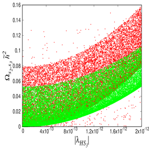
(a)

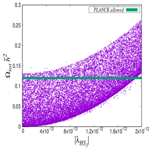
(b)

Figure 3: The variations of the relic abundances $\Omega_{s_{2},s_{3}}{\tilde{h}}^{2}$ for each of the two DM components with the coupling $\lambda_{HS_{3}}$. The red and green regions represent the relic abundaces of $s_{2}$ and $s_{3}$ respectively. Right panel shows the variation of $\Omega_{\rm tot}{\tilde{h}}^{2}$ with $\lambda_{HS_{3}}$. The PLANCK limit is shown by the thick green line. See text for details.

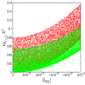
(a)

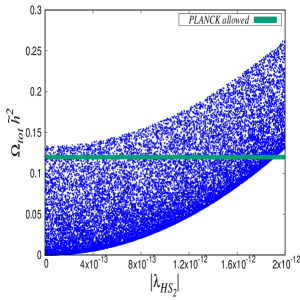
(b)

Figure 4: Same as Fig. 3 but for $\lambda_{HS_{2}}$.

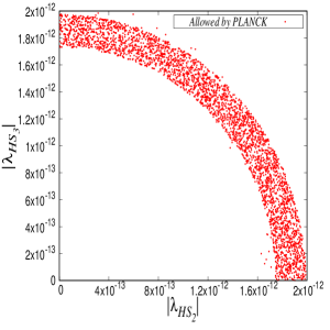
Figure 5: The available region constrained by the PLANCK results in $\lambda_{HS_{2}}-\lambda_{HS_{3}}$ plane is denoted in this figure.

Unlike the WIMP dark matter where the relic density of dark matter would decrease with the increase of the Higgs-couplings with the DM candidates, for the case of FIMP DM the relic density increases with the Higgs-couplings instead. This is one of the salient features of FIMP dark matter. This can also be seen from Figs. 3,4 that the nature of variations of the relic abundances with $\lambda_{HS_{i}}(i=2,3)$ are parabolic which reflect the fact that $\Omega{\tilde{h}}^{2}\sim\lambda_{HS_{i}}^{2}(i=2,3)$.

Further, in order to constrain the parameter space by the PLANCK observational results we simultaneously vary the two parameters $\lambda_{HS_{2}},\lambda_{HS_{3}}$. The results are plotted in Fig. 6. In Fig. 6 we show the two parameter scan results, where the region constrained by the PLANCK results are shown by the red colour zone in the $\lambda_{HS_{2}}-\lambda_{HS_{3}}$ plane.

6.2 FIMP at MeV Mass Regime

In the MeV regime we choose the masses of the two component dark matter to be 10 MeV and 5 MeV. With these masses and using our formalism of two component FIMP dark matter model we constrain the parameter space following the procedures similar to what described in Section 6.1. In this mass region too the parameter space is finally constrained by calculating the relic abundance and then comparing them with the PLANCK results. The results are shown in Figs. 6,7. From Fig. 6 and Fig. 7 which show the variations of relic abundances for each of the two components as well as the total abundance with the coupling parameters $\lambda_{HS_{2}},\lambda_{HS_{3}}$ respectively we obtain an upper limit for $\lambda_{HS_{3}}$ and $\lambda_{HS_{2}}$ to be of the order of $\sim 8\times 10^{-11}$. In Fig. 8 we show the parameter space restricted by the PLANCK relic abundance results and is indicated by the red colour region in the relevant plot.

6.3 FIMP at keV Mass Regime

In the keV range we have considered the masses of the two FIMP scalar components to be 10 keV and 5 keV and performed the analysis similar to what described in the cases of GeV and MeV ranges for restricting the parameter space. The results are shown in Figs. 9,10. We find similar nature for variations of the relic abundances with the couplings (Figs. 9,10) as also for the constrained parameter space (Fig. 11). We find the upper limits for $\lambda_{HS_{3}}$ and $\lambda_{HS_{2}}$ to be around $2.2\times 10^{-9}$.

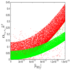
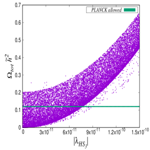
Figure 6: Same as Fig. 3 but for MeV mass regime. See text for details.

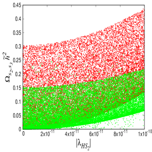
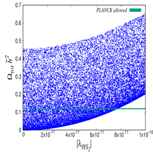
Figure 7: Same as Fig. 4 but for MeV mass regime.

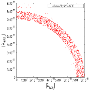
Figure 8: Same as Fig. 5 but for MeV mass regime.

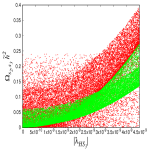
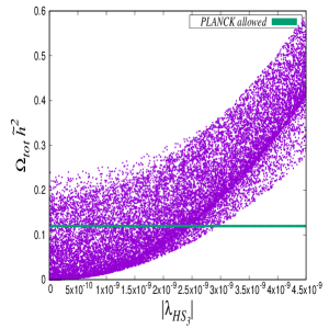
Figure 9: Same as Fig. 3 but for keV mass regime. See text for details.

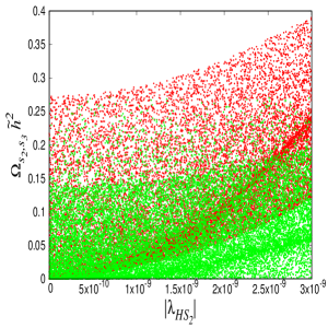
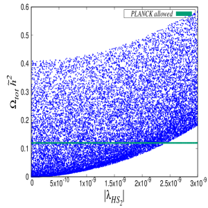
Figure 10: Same as Fig. 4 but for keV mass regime.

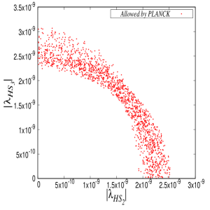
Figure 11: Same as Fig. 5 but for keV mass regime.

7 Self Interactions for Singlet Scalar Dark Matter

Recently there are evidences of dark matter self interactions [58, 70, 71, 72, 73] from the observations of collision of several galaxy clusters. The visible part of a galaxy is generally embedded inside a spherical halo of dark matter that extends far beyond the visible reaches of that galaxy. The dark matter halo makes up most of the galaxy masses. At the time of collisions between multiple galaxies a lareger galaxy among them pulls stars and other stellar material from a smaller galaxy and this process is called tidal stripping. Due to the presence of gravitational effect one galaxy pulls in material from another and this can cause the dark matter to suffer a spatial offset from the stars in the galaxy. Recently the galaxy cluster Abell 3827 is observed by the Hubble Space Telescope [71]. The observations of the four elliptical galaxies falling into the inner 10 Kpc core of galaxy cluster Abell 3827 indicate that the dark matter could be self interacting. The position of the dark matter halos of the four falling galaxies can be restored by using gravitational lensing and many other strongly - lensed images of background objects. It is observed that one of the halos among these four galaxies is significantly separated from its stars by a distance of $\Delta=1.62^{+0.47}_{-0.49}$ Kpc. This spatial offset can be explained by the study of dark matter self interaction. Determination of the size of the spatial offset gives us an estimate of this self interaction cross-section to the $\sigma_{\rm DM}/m\sim 1.5\,\rm{cm}^{2}/\rm{g}$ which is consistent with the bound obtained from [58]. A study on 72 colliding galaxy clusters [58] also put an upper limit on the self interaction cross-section as $\sigma_{\rm DM}/m<0.47\,\rm{cm}^{2}/\rm{g}$ with 95$\%$ C.L. It appears from [72] that for the singlet scalar dark matter produced via thermal freeze-out mechanism cannot explain the observed DM self-interaction cross-section. The DM candidates produced via thermal freeze-in mechanism might explain the DM self interactions deduced from the observational results mentioned above. In our model, as discussed earlier, we have proposed two scalar DM candidates (two component scalar DM) $s_{2}$ and $s_{3}$ in FIMP scenario.

Under the framework of present model the self interaction scattering cross-section per unit dark matter mass ($\sigma/m_{s}$) for singlet scalar dark matter can be wriiten as [72],

$$\frac{\sigma}{m_{s}}\simeq\frac{9\lambda^{2}}{2\pi m_{s}^{3}}\,\,\,,$$ (48)

where $\lambda=\lambda_{S}$ for mass of dark matter to be much higher than mass of Higgs and $\lambda=\lambda_{S}-{g^{2}\over 8m_{h}^{2}}$ [72] when mass of dark matter is less than that of Higgs. Here, $\lambda_{S}$ and $g$ denote the 4-point dark matter self-coupling and the coupling of Higgs to the dark matter respectively. We coinsider $g\leq 2\pi$ in our work. Also $m_{s}$ and $m_{h}$ are the corresponding masses of dark matter and the Higgs. In case of two scalar singlet model the above relation is modified and the effective scattering cross-section per unit effective dark matter mass can be expressed as,

$$\frac{\sigma}{m}\bigg{|}_{\rm eff}=f^{2}_{s_{2}}\frac{9\lambda_{S_{2}}^{2}}{2\pi m_{s_{2}}^{3}}+f^{2}_{s_{3}}\frac{9\lambda_{S_{3}}^{2}}{2\pi m_{s_{3}}^{3}}+f_{s_{2}}f_{s_{3}}\frac{9\lambda_{S_{2}S_{3}}^{2}}{2\pi\mu_{s}^{3}}\,\,\,,$$ (49)

where $\lambda_{S_{2}}$, $\lambda_{S_{3}}$ denote the 4-point self couplings among each of $s_{2}$, $s_{3}$ respectively while $\lambda_{S_{2}S_{3}}$ denotes the same between $s_{2}$ and $s_{3}$. In Eq. (49) $f_{s_{2}}$ and $f_{s_{3}}$ are respectively the corresponding dark matter density fractions $f_{i}=\frac{\Omega_{i}}{\Omega_{\rm DM}}\,\,,i=s_{2},s_{3}$ [66, 74] for $s_{2}$ and $s_{3}$. Since $f_{s_{2}}+f_{s_{3}}=1(f_{s_{2}}=1-f_{s_{3}})$, Eq. (49) reduces to the form

$$\frac{\sigma}{m}\bigg{|}_{\rm eff}=f_{s_{2}}^{2}\left(\frac{9\lambda_{S_{2}}^{2}}{2\pi m_{s_{2}}^{3}}+\frac{9\lambda_{S_{3}}^{2}}{2\pi m_{s_{3}}^{3}}-\frac{9\lambda_{S_{2}S_{3}}^{2}}{2\pi\mu_{s}^{3}}\right)+f_{s_{2}}\left(\frac{9\lambda_{S_{2}S_{3}}^{2}}{2\pi\mu_{s}^{3}}-2\frac{9\lambda_{S_{3}}^{2}}{2\pi m_{s_{3}}^{3}}\right)+\frac{9\lambda_{S_{3}}^{2}}{2\pi m_{s_{3}}^{3}}\,\,\,.$$ (50)

Using the observational bounds on $\frac{\sigma}{m}\bigg{|}_{\rm eff}$ one may restrict the parameter space $f_{s_{2}}-m_{s_{2}}-m_{s_{3}}$ from Eq. (50). For this purpose upper bounds on the couplings $\lambda_{S_{2}}$, $\lambda_{S_{3}}$ and $\lambda_{S_{2}S_{3}}$ from perturbative unitarity conditions are used and $\frac{\sigma}{m}$ is calculated using Eq. (50) for a range of masses $m_{s_{2}}$ and $m_{s_{3}}$ for the two components with different fixed chosen values of $f_{s_{2}}$ ($0<f_{s_{2}}<1$). In Fig. 12 we plot for diferent $f_{2}$ values those pairs of $m_{S_{2}}$ and $m_{S_{3}}$ in $m_{S_{2}}-m_{S_{3}}$ in plane that satisfy the limit $\frac{\sigma}{m}=0.47$. Thus, in addition to the constraints described in Sect. 4, the self interaction results will further constrain the masses of the dark matter components. The plots in Fig. 12 show the upper bounds on the masses of dark matter for different fixed $f_{s_{2}}$ values.

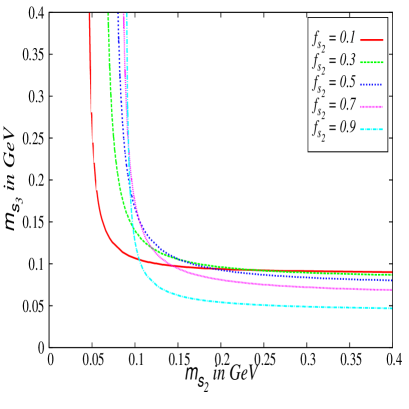
Figure 12: The upper limits for the masses of the scalar components $m_{s_{2}}$ and $m_{s_{3}}$ that satisfy the dark matter self interaction limit (from observations) for different chosen values of fractional densities of $s_{2}$ component. See text for details.

Each pair of points on a plot in Fig. 12 for a fixed value of $f_{s_{2}}$ therefore correspond to the upper limit of the masses for the components $s_{2}$ and $s_{3}$ that satisfy the self interaction observational upper bound given in Eq. (49). The left region of each such plot in Fig. 13 therefore describes the allowed region for the masses of $s_{2}$ and $s_{3}$ for a chosen fractional density ($f_{s_{2}}$ and therefore $f_{s_{3}}=(1.0-f_{s_{2}})$). From these plots of Fig. 12 it reveals that there are upper bounds of masses for each of the scalar components beyond which the experimental bound for $\sigma/m$ will not be satisfied. Moreover, it can also be seen that the maximum values of $m_{s_{2}}$ and $m_{s_{3}}$ (for the chosen maximum value of $\frac{2\pi}{3}$ for the couplings) do not exceed $\sim 0.2$ GeV. These maximum limits of the individual masses $m_{s_{2}}$ or $m_{s_{3}}$ also vary for different fractional densities $f_{s_{2}}$ ($f_{s_{3}}$) of the respective components. For example, for $f_{s_{2}}=0.3$ ($f_{s_{3}}=0.7$), the mass of the $s_{2}$ component does not exceed a value $\sim 0.06$ GeV while the mass of the $s_{3}$ component remains limited to a value of around 0.15 GeV. Again, for $f_{s_{2}}=0.9$ ($f_{s_{3}}=0.1$) $-$ a situation when the two component dark matter is overwhelmingly dominated by only the $s_{2}$ component $-$ the upper limit for $m_{s_{2}}\sim 0.11$ GeV. Similar results, but for just one component dark matter scenario is given earlier by Campbell et al [72]. Here we show, for the case of a two component scalar FIMP dark matter model, the simultaneous limits for the masses of the two components restricted by the self interaction bounds. It is also to be noted that although a FIMP dark matter scenario appears to be viable candidate in the mass range as high as few GeV from the present analysis of Sect. 6, such mass range is disallowed from self interaction considerations.

8 Summary and Discussions

The key feature of FIMP dark matter is that they were never in thermal equilibrium to the Universe’s heat bath and are produced non-thermally while they approach their ”freeze-in” density. Their couplings with SM particles are so feeble that they never attempt thermal equilibrium. But these types of feebly coupled dark matter may have significance in cosmological or astrophysical contexts such as formation of small scale structures, signatures of the primordial initial conditions present in the Universe or to address issues like “too big to fail problem” etc.

In this work we extend the scalar sector of Standard Model by introducing two singlet scalars where these scalars are considered to have produced in the early Universe via Feebly Interacting Massive Particle or FIMP mechanism. We perform extensive phenomenology of such a model and show that our two component FIMP scalars can be a viable candidate for dark matter in the Universe. Using the theoretical constraints on the interaction potential as well as the couplings as also employing the PLANCK observed relic densities and collider bounds, we domonstrate that in FIMP scenario, the mass regime of such scalar FIMP dark matter candidates may extend from GeV to keV. We have also explored the self interaction for these dark matter candidates. The self interaction cross section bound obtained from the results of 72 colliding galaxy clusters however restricts the viable mass range to upper values of around $\sim 0.2$ GeV.

A FIMP dark matter has various cosmological and astrophysical implications as well as implications on its direct and indirect signatures [75]. As the couplings of such candidates are extremely small it is difficult to obtain measurable direct signatures arising out of elastic scattering or indirect signatures from annihilation of FIMP dark matter. However, signals from decay of nonthermal light dark matter in the form of observed X-ray signals (3.55 keV line [76]) have been explored previously by one of the present authors [77]. The issues such as small scale structure formation problems can be addressed by warm dark matter with non thermal velocity distribution which is possible if they are produced via “freeze-in” mechanism [75]. As the FIMP dark matter never attains thermal equilibrium due to their feeble coupling, the initial condition for such non thermal production at early Universe is not washed away and can be probed via FIMP dark matter studies. Any primordial fluctuations caused by very feeble interactions of scalar fields in dark sector (which may not be washed away to absence of thermalisation) can be probed by their possible imprints in Cosmic Microwave Radiation (CMB).

The FIMP dark matter therefore has wide implications not only in addressing various dark matter related issues but other astrophysical and cosmological concerns as well as the particle nature of dark matter. A two component or multicomponent dark matter in this scenario may be useful to probe simultaneously various aspects related to dark matter ranging from cosmology or astrophysics to particle physics.

Acknowledgements

The authors thank A. Dutta Banik and A. Biswas for their useful comments and suggestions. The authors would also like to thank Dr. Tommi Tenkanen for his useful suggestions. One of the authors (MP) thanks the DST-INSPIRE fellowship grant by DST, Govt. of India.

Appendix

The expressions for the couplings used in this work are listed below

$$g_{hhh} = -\lambda_{H}v\,\,,$$

$$g_{hs_{2}s_{2}} = -\lambda_{HS_{2}}v\,\,,$$

$$g_{hs_{3}s_{3}} = -\lambda_{HS_{3}}v\,\,,$$

$$g_{hhs_{2}s_{2}} = -\displaystyle\frac{\lambda_{HS_{2}}}{2}\,\,,$$

$$g_{hhs_{3}s_{3}} = -\displaystyle\frac{\lambda_{HS_{3}}}{2}\,\,,$$

$$g_{s_{2}s_{2}s_{3}s_{3}} = -\lambda_{S_{2}S_{3}}\,\,,$$

$$g_{s_{2}s_{2}s_{2}s_{2}} = -\displaystyle\frac{\lambda_{S_{2}}}{4}\,\,,$$

$$g_{s_{3}s_{3}s_{3}s_{3}} = -\displaystyle\frac{\lambda_{S_{3}}}{4}\,\,,$$

$$g_{WWh} = \displaystyle\frac{2m^{2}_{W}}{v}\,\,,$$

$$g_{ZZh} = \displaystyle\frac{m^{2}_{Z}}{v}\,\,,$$

$$g_{ffh} = \displaystyle\frac{m_{f}}{v}\,\,.$$

References

- [1] Y. Sofue and V. Rubin, Ann. Rev. Astron. Astrophys. 39, 137 (2001).
- [2] M. Bartelmann and P. Schneider, Phys. Rept. 340, 291 (2001).
- [3] D. Clowe, A. Gonzalez and M. Markrvitch, Astrophys. J. 604, 595 (2004).
- [4] P. A. R. Ade et al. [PLANCK Collaboration], Astron. Astrophys. 571, A16 (2014).
- [5] D. S. Akerib et al., arXiv:1608.07648 [astro-ph.CO].
- [6] E. Aprile et al. [XENON Collaboration], JCAP 1604, no. 04, 027 (2016).
- [7] A. Tan et al. [PandaX-II Collaboration], Phys. Rev. Lett. 117, no. 12, 121303 (2016).
- [8] G. Jungman, M. Kamionkowski and K. Griest, Phys. Rept. 267, 195 (1996).
- [9] K. Griest and M. Kamionkowski, Phys. Rept. 333, 167 (2000).
- [10] G. Bertone, D. Hooper and J. Silk, Phys. Rept. 405, 279 (2005).
- [11] H. Murayama, arXiv: 0704.2276 [hep-ph].
- [12] P. Gondolo and G. Gelmini, Nucl. Phys. B 360, 145 (1991).
- [13] M. Srednicki, R. Watkins and K. A. Olive, Nucl. Phys. B 310, 693 (1988).
- [14] H. C. Cheng, J. L. Feng and K. T. Matchev, Phys. Rev. Lett. 89, 211301 (2002) [hep-ph/0207125]; G. Servant and T. M. P. Tait, Nucl. Phys. B 650, 391 (2003) [hep-ph/0206071].
- [15] V. Silveira and A. Zee, Phys. Lett. B 161, 136 (1985).
- [16] J. McDonald, Phys. Rev. D 50, 3637 (1994).
- [17] C. P. Burgess, M. Pospelov and T. ter Veldhuis, Nucl. Phys. B 619, 709 (2001).
- [18] V. Barger, P. Langacker, M. McCaskey, M. J. Ramsey-Musolf and G. Shaughnessy, Phys. Rev. D 77, 035005 (2008).
- [19] E. Ma, Phys. Rev. D 73, 077301 (2006).
- [20] L. Lopez Honorez, E. Nezri, J. F. Oliver and M. H. G. Tytgat, JCAP 0702, 028 (2007).
- [21] D. Majumdar and A. Ghosal, Mod. Phys. Lett. A 23, 2011 (2008).
- [22] M. Gustafsson, E. Lundstrom, L. Bergstrom and J. Edsjo, Phys. Rev. Lett. 99, 041301 (2007).
- [23] E. Lundstrom, M. Gustafsson and J. Edsjo, Phys. Rev. D 79, 035013 (2009).
- [24] S. Andreas, M. H. G. Tytgat and Q. Swillens, JCAP 0904, 004 (2009).
- [25] L. Lopez Honorez and C. E. Yaguna, JHEP 1009, 046 (2010).
- [26] L. Lopez Honorez and C. E. Yaguna, JCAP 1101, 002 (2011).
- [27] T. A. Chowdhury, M. Nemevsek, G. Senjanovic and Y. Zhang, JCAP 1202, 029 (2012).
- [28] D. Borah and J. M. Cline, Phys. Rev. D 86, 055001 (2012).
- [29] A. Arhrib, R. Benbrik and N. Gaur, Phys. Rev. D 85, 095021 (2012).
- [30] A. Goudelis, B. Herrmann and O. Stål, JHEP 1309, 106 (2013).
- [31] A. D. Banik and D. Majumdar, Eur. Phys. J. C 74, no. 11, 3142 (2014).
- [32] Y. G. Kim, K. Y. Lee and S. Shin, JHEP 0805, 100 (2008).
- [33] M. M. Ettefaghi and R. Moazzemi, JCAP 1302, 048 (2013).
- [34] M. Fairbairn and R. Hogan, JHEP 1309, 022 (2013).
- [35] T. Hambye, JHEP 0901, 028 (2009).
- [36] C. H. Chen and T. Nomura, Phys. Lett. B 746, 351 (2015).
- [37] S. Di Chiara and K. Tuominen, JHEP 1511, 188 (2015).
- [38] M. Heikinheimo, T. Tenkanen, K. Tuominen, Phys. Rev. D 96, 023001 (2017).
- [39] A. Karam and K. Tamvakis, Phys. Rev. D 92, no. 7, 075010 (2015).
- [40] A. Karam and K. Tamvakis, Phys. Rev. D 94, no. 5, 055004 (2016).
- [41] A.D. Banik, D. Majumdar and A. Biswas, Eur. Phys. J. C. 76, no. 6, 346 (2016).
- [42] G. Arcadi et al, [arXiv:1703.07364[hep-ph]].
- [43] J. McDonald, Phys. Rev. Lett. 88, 091304 (2002).
- [44] L. J. Hall, K. Jedamzik, J. March-Russell and S. M. West, JHEP 1003, 080 (2010).
- [45] S. Nurmi, T. Tenkanen and K. Tuominen, JCAP 11, 001 (2015).
- [46] P.S.B. Dev, A. Mazumdar and S. Qutub, Front. Phys. 2, 26 (2014).
- [47] A. Merle and A. Schneider, Phys. Lett. B 749, 283 (2015).
- [48] A. Merle and M. Totzauer, JCAP 1506, 011 (2015).
- [49] B. Shakya, Mod. Phys. Lett. A 31, no. 06, 1630005 (2016).
- [50] A. Biswas and A. Gupta, JCAP 1609, no. 09, 044 (2016).
- [51] R. Campbell, S. Godfrey, H. E. Logan, A. D. Peterson and A. Poulin, Phys. Rev. D 92, no. 5, 055031 (2015).
- [52] M. Kaplinghat, T. Linden and H. B. Yu, Phys. Rev. Lett. 114, no. 21, 211303 (2015).
- [53] A. Biswas and A. Gupta, arXiv:1612.02793 [hep-ph].
- [54] K.P. Modak, D. Majumdar and S. Rakshit, JCAP, 1503 (2015) [arXiv:1312.7488v2[hep-ph]].
- [55] S. Bhattacharya, P. Ghosh and P. Poulose, JCAP (2017) [arXiv:1607.08461[hep-ph]].
- [56] S. Bhattacharya, P. Ghosh, T.N. Maity, T.S. Ray, [arXiv:1706.04699[hep-ph]].
- [57] G. Hinshaw et al. [WMAP Collaboration], Astrophys. J. Suppl. 208, 19 (2013).
- [58] D. Harvey, R. Massey, T. Kitching, A. Taylor and E. Tittley, Science 347, 1462 (2015).
- [59] K. Kannike, Eur. Phys. J. C 72, 2093 (2012).
- [60] B.W. Lee, C. Quigg and H.B. Thacker, Phys. Rev. D 16, 1519 (1977).
- [61] G. Aad et al. [ATLAS Collaboration], Phys. Lett. B 716, 1 (2012).
- [62] S. Chatrchyan et al. [CMS Collaboration], Phys. Lett. B 716, 30 (2012).
- [63] G. Belanger, B. Dumont, U. Ellwanger, J. F. Gunion and S. Kraml, Phys. Lett. B 723, 340 (2013).
- [64] [ATLAS Collaboration], ATLAS-CONF-2012-162.
- [65] M. Heikinheimo, T. Tenkanen, K. Tuiminen, V. Vaskonen, Phys. Rev. D 94, 063506 (2016).
- [66] A.D. Banik, M. Pandey, D. Majumdar and A. Biswas, Eur. Phys. J. C 77, 657 (2017). [arXiv:1612.08621v1[hep-ph]].
- [67] N. Bernal, X. Chu, JCAP 1601, 006 (2016).
- [68] J. Edsjo and P. Gondolo, Phys. Rev. D 56, 1879 (1977) [hep-ph/9704361]
- [69] A. Biswas and D. Majumdar, Pramana 80, 539 (2013) [arXiv:1102.3024 [hep-ph]].
- [70] D. Harvey ffet al., Mon. Not. Roy. Astron. Soc. 441, no. 1, 404 (2014).
- [71] F. Kahlhoefer, K. Schmidt-Hoberg, J. Kummer and S. Sarkar, Mon. Not. Roy. Astron. Soc. 452, no. 1, L54 (2015).
- [72] R. Campbell, S. Godfrey, H. E. Logan, A. D. Peterson and A. Poulin, Phys. Rev. D 92, no. 5, 055031 (2015).
- [73] M. Kaplinghat, T. Linden and H. B. Yu, Phys. Rev. Lett. 114, no. 21, 211303 (2015).
- [74] M. Mrkevitch et al., Astrophys. J. 606, 819 (2004).
- [75] N. Bernal, M. Heikinheimo, T. Tenkanen, K. Tuominen and V. Vaskonen, [arXiv:1706.07442[hep-ph]].
- [76] E. Bulbul, M. Markevitch, A. Foster, R. K. Smith, M. Loewenstein and S. W. Randall, Astrophys. J. 789, 13 (2014).
- [77] A. Biswas, D. Majumdar and P. Roy, Europhys. Lett. 113. no. 2, 29001 (2016).