A General Framework for Flexible
Multi-Cue Photometric Point Cloud Registration

Abstract

The ability to build maps is a key functionality for the majority of mobile robots. A central ingredient to most mapping systems is the registration or alignment of the recorded sensor data. In this paper, we present a general methodology for photometric registration that can deal with multiple different cues. We provide examples for registering RGBD as well as 3D LIDAR data. In contrast to popular point cloud registration approaches such as ICP our method does not rely on explicit data association and exploits multiple modalities such as raw range and image data streams. Color, depth, and normal information are handled in an uniform manner and the registration is obtained by minimizing the pixel-wise difference between two multi-channel images. We developed a flexible and general framework and implemented our approach inside that framework. We also released our implementation as open source C++ code. The experiments show that our approach allows for an accurate registration of the sensor data without requiring an explicit data association or model-specific adaptations to datasets or sensors. Our approach exploits the different cues in a natural and consistent way and the registration can be done at framerate for a typical range or imaging sensor.

I Introduction

Most mobile robots need to estimate a map of their surroundings in order to navigate. Thus, the task of registering the incoming sensor data such as images or point clouds is an important building block for most autonomous systems. This functionality is also of key importance for estimating the relative motion of a robot through incremental matching, often called visual odometry or laser-based odometry, depending on the used sensing modality.

We investigate the problem of registering data from typical robotic sensors such as the Kinect camera, a 3D LIDAR such as a Velodyne laser scanner, or similar in a general way without requiring special, sensor-specific adaptations. More concretely our goal is to provide a general methodology to find the transformation that maximizes the overlap between two measurements taken from the same scene.

To this extent, ICP is a popular strategy for registering point clouds. It proceeds by iteratively alternating two steps: data association and transform estimation. Data association computes pairs of corresponding points in the two clouds, while transform estimation calculates an isometry that applied to one of the two clouds minimizes the distance between corresponding points. The weakness of ICP lies in the correspondence search as this step usually relies on heuristics and may introduce biases or gross errors.

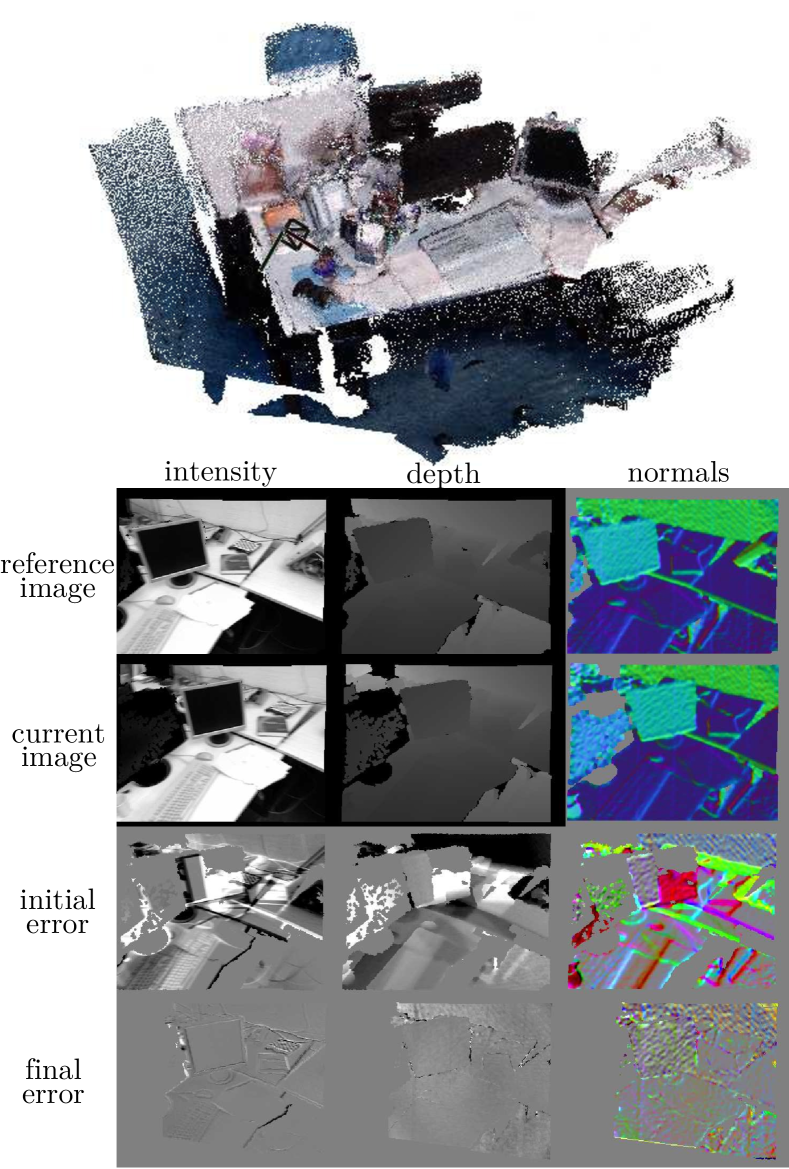
Figure 1: Our approach realized an effective multi-cue registration without requiring features nor an explicit data association between features or 3D points.

Over time, effective variants of ICP that exploit the structure of the scene have been proposed [12, 14]. Using the structure either by relying on a point-to-plane or a plane to plane metric has been shown to improve the performance of the algorithm, especially in indoor/structured environments. Kerl et al. [9] recently proposed Dense Visual Odometry (DVO), an approach to register RGBD images by minimizing the photometric distance. The idea is to find the location of a camera within a scene such that the image captured at that location is as close as possible to the measured RGBD image. By exploiting the image gradients, DVO does not require explicit data association, and it is able to achieve unprecedented accuracy. The main shortcoming of DVO is that it is restricted to the use of depth/intensity image pairs. In its original formulation DVO does not naturally incorporate additional structural cues such as normals or curvature. The use of these cues has been shown to substantially enlarge the basin of convergence and reduce the number of iterations needed to find a solution.

The main contribution of this paper is a general methodology to photometric sensor data registration that works on cues such as color, depth, and normal information in a unified way and does not require an explicit data association between features, 3D points, or surfaces. The approach is inspired by DVO [9]. It does not require any feature extraction, and operates directly on the image or image-like data obtained from a sensor such as the Kinect or a 3D LIDAR. A key property of our approach is an easy-to-extend, mathematically sound framework for registration that does not need to make an explicit data association between sensor readings or the 3D model. In contrast, it solves the registration problem as a minimization in the color, depth, and normal data exploiting projections of the sensor data. It can be seen as a generalization of DVO to handle arbitrary cues and multiple sensing modalities in a flexible way. An example of this registration is illustrated in Fig. 1. We provide an open source C++ implementation at:

https://gitlab.com/srrg-software/srrg_mpr

In sum, we make the following key claims: Our approach (i) is a general methodology for photometric registration that works transparently with different sensor cues and avoids an explicit point-to-point or point-to-surface data association, (ii) can accurately register typical sensor cues such as RGBD Kinect or LIDAR data exploiting the color, depth, and normal information, (iii) robustly computes the transformation between view points under realistic disturbances of the initial guess, and (iv) can be executed fast enough to allow for online processing of the sensor data without sensor-specific optimizations. These four claims are backed up through the experimental evaluation.

II Related Work

There exist a large number of different registration approaches. One general way for aligning 3D point clouds is the ICP algorithm, which has often been used in the context of range data. Popular approaches use ICP together with point-to-point or point-to-plane correspondences [5] and generalized variants such as GICP [12]. There exist approaches exploiting normal information such as NICP [15] as well as global approaches [19] that use branch-and-bound technique coupled with standard ICP formulation. A popular and effective approach is LOAM [20, 21] by Zhang and Singh that extracts distinct surface and corner features from the point cloud and determine plane-to-point and line-to-point distances to a voxel-grid representation.

Traditional approaches to visual odometry track sparse features in monocular images or stereo pair to estimate the relative orientation of the images [3, 11]. To deal with outliers in the data association between feature points, most approaches use RANSAC to identify inlier and outlier points, combined with a tracking over multiple frames. Other approaches rely on a prior for the motion estimate, such as constant motion model. In presence of external sensors, such as an IMU, the measurements can be filtered with the achieved motion estimate [1, 22].

Another group of approaches exploits the depth data from RGBD streams to register scans and build dense models of the scene. KinectFusion by Newcombe et al. [10], for example, largely impacted the RGBD SLAM developments over the last 6 years. Similar to Newcombe et al., the approach of Keller et al. [6] uses projective data association for RGBD SLAM in a dense model and relies on a surfel-based map [18] for tracking. Similar approaches exploit the RGBD streams by defining signed distance fields where a direct voxel-based difference is computed to perform the motion estimation [16], making intense use of both CPU and GPU parallelization. ICP is a frequently used approach for RGBD data and special variants for denser depth images have been proposed [14, 15]. Recently, the team around Daniel Cremers has proposed semi-dense approaches using image data [2] to solve the visual odometry and SLAM problem as well as dense approaches for featureless visual odometry for RGBD data [7, 8, 9].

In this paper we propose a general and easy-to-implement methodology for multi-cue photometric registration of 3D point clouds that can be seen as an extension of DVO. In contrast to nearly all previous works, our method has been designed without considering a specific sensor, nor a particular cue, as we aim to apply the same exact algorithm in several contexts.

III Approach

Our approach seeks to register either two observations with respect to each other or an observation against a 3D model. The sensor observations are assumed to have a 2D representation $\boldsymbol{\mathfrak{I}}$ such as an image from a regular camera, a range image from a depth camera or a 3D LIDAR, or a similar type of observation. Such a 2D measurement can be seen as an image, where each pixel in the image plane contains one or more channels, i.e., $\boldsymbol{\mathfrak{I}}=\{\boldsymbol{\mathfrak{I}}^{\mathrm{c}}\}$ with the channel index $c$. Examples of such channels are light intensity, depth information, or surface normals.

We aim at registering the current observation to a model, for which 3D information is available in form of a point cloud. This model can be a given 3D model, or a point cloud estimated from the previous observation(s). We refer to it as the model cloud $\mathcal{M}=\{\mathbf{p}\}$. In addition to the 3D coordinates, each point $\mathbf{p}\in\mathcal{M}$ can also store multiple cues such as light intensity or a surface normal.

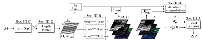
Figure 2: Key ingredients of our framework and links to the corresponding subsections.

The following subsections describe the key ingredients of our approach, see also Fig. 2 for an illustration. Sec. III-A presents the overall error minimization formulation that uses three functions, which are sensor and/or cue-specific and must be implemented by the user when adding a new cue or a different sensor, everything else is handled by our framework. These functions are:

• Sec. III-B: Cue-specific mapping function $\mathrm{map}^{\mathrm{c}}()$ that describes if and how a cue is transformed through a coordinate transformation.

• Sec. III-C: Projection model $\mathrm{proj}()$ of the sensor, e.g., the pinhole camera model

• Sec. III-E: The corresponding Jacobians

III-A Photometric Error Minimization

As in photometric error minimization approaches, our method seeks to iteratively minimize the pixel-wise difference between the current image $\boldsymbol{\mathfrak{I}}$ and the predicted image $\hat{\boldsymbol{\mathfrak{I}}}(\mathcal{M},\mathbf{X})$. Here, $\hat{\boldsymbol{\mathfrak{I}}}(\mathcal{M},\mathbf{X})$ is a multi-channel image obtained by projecting the model $\mathcal{M}$ onto a virtual camera located at a pose $\mathbf{P}_{\mathbf{X}}$, where $\mathbf{X}$ is a transformation matrix that transforms the points of $\mathcal{M}$ from the global into the local camera coordinate system. More formally, our method seeks to minimize

$$\mathbf{X}^{*} = \operatorname*{argmin}_{\mathbf{X}}\sum_{u,v,\mathrm{c}}\|\underbrace{\hat{\boldsymbol{\mathfrak{I}}}^{\mathrm{c}}_{u,v}(\mathcal{M},\mathbf{X})-\boldsymbol{\mathfrak{I}}^{\mathrm{c}}_{u,v}}_{\mathbf{e}^{\mathrm{c}}_{u,v}(\mathcal{M},\mathbf{X})}\|^{2}_{\mathbf{\Omega}^{\mathrm{c}}}$$ (1)

$$= \operatorname*{argmin}_{\mathbf{X}}\sum_{u,v,\mathrm{c}}{\mathbf{e}^{\mathrm{c}}_{u,v}(\mathcal{M},\mathbf{X})}^{\top}\,\mathbf{\Omega}^{\mathrm{c}}\,\mathbf{e}^{\mathrm{c}}_{u,v}(\mathcal{M},\mathbf{X})$$ (2)

where $\mathbf{e}^{\mathrm{c}}_{u,v}(\mathcal{M},\mathbf{X})$ denotes an error at a pixel location ${(u~{}v)}^{\mathrm{T}}$ between the predicted value $\hat{\boldsymbol{\mathfrak{I}}}^{\mathrm{c}}_{u,v}(\mathcal{M},\mathbf{X})$ and the measured one $\boldsymbol{\mathfrak{I}}^{\mathrm{c}}_{u,v}$ for a particular channel index $c$. The matrix $\mathbf{\Omega}=\mathrm{diag}(\{{\mathbf{\Omega}^{\mathrm{c}}}\})$ is a block diagonal information matrix used to weight the different channels of the image.

Let $\mathcal{M}_{\mathrm{vis}}$ be the subset of points from the model $\mathcal{M}$ that are visible from the image plane of image $\boldsymbol{\mathfrak{I}}$. In our current implementation, we construct this set using the depth buffer as explained in details in Sec. III-D. Given $\mathcal{M}_{\mathrm{vis}}$, we can rewrite the sum in Eq. (1) using the points:

$$\mathbf{X}^{*} = \operatorname*{argmin}_{\mathbf{X}}\sum_{\mathrm{c},\mathbf{p}\in\mathcal{M}_{\mathrm{vis}}}\left\|\mathbf{e}^{\mathrm{c}}_{\mathbf{p}}(\mathbf{X})^{\top}\right\|^{2}_{\mathbf{\Omega}^{\mathrm{c}}}.$$ (3)

Each point-wise error term $\mathbf{e}^{\mathrm{c}}_{\mathbf{p}}(\mathbf{X})^{\top}$ is the difference between a predicted and a measured channel evaluated at the pixel where the point $\mathbf{p}$ projects onto given the model of the sensor. We expand the point-wise error as follows:

$$\mathbf{e}^{\mathrm{c}}_{\mathbf{p}}(\mathbf{X}) = \mathrm{map}^{\mathrm{c}}(\mathbf{X},\mathbf{p})-\boldsymbol{\mathfrak{I}}^{\mathrm{c}}_{\mathrm{proj}(\mathbf{X}\,\mathbf{p})}.$$ (4)

The term $\mathrm{proj}(\mathbf{X}\,\mathbf{p})={(u~{}v)}^{\mathrm{T}}$ is a function that computes the image coordinates obtained by projecting the point $\mathbf{p}$ onto a camera located at $\mathbf{P}_{\mathbf{X}}$. The function $\mathrm{map}^{\mathrm{c}}(\mathbf{X},\mathbf{p})$ computes the value of channel $\hat{\boldsymbol{\mathfrak{I}}}^{\mathrm{c}}(\mathcal{M},\mathbf{X})$ evaluated at the pixel $\mathrm{proj}(\mathbf{X}\,\mathbf{p})$. During a first read, that may sound confusing as the default cue light intensity is not affected by the transformation and are simply copied from the information in the point $\mathbf{p}$. Other cues, however, such as normals or depth values are viewpoint-dependent and therefore change depending on the given camera pose $\mathbf{P}_{\mathbf{X}}$.

Our approach minimizes Eq. (3) by using a regularized least squares optimization procedure. Combining Eq. (3) with Eq. (4) and adding a per-point regularization weight $w_{\mathbf{p}}$, we can rewrite Eq. (1) in terms of points as

$$\mathbf{X}^{*}=\operatorname*{argmin}_{\mathbf{X}}\sum_{\mathbf{p}\in\mathcal{M}_{\mathrm{vis}}}w_{\mathbf{p}}\sum_{\mathrm{c}}\|\mathrm{map}^{\mathrm{c}}(\mathbf{X},\mathbf{p})-\boldsymbol{\mathfrak{I}}^{\mathrm{c}}_{\mathrm{proj}(\mathbf{X}\,\mathbf{p})}\|^{2}_{\mathbf{\Omega}^{\mathrm{c}}},$$ (5)

where the regularization weight $w_{\mathbf{p}}$ decreases with the magnitude of the channel errors $\mathbf{e}^{\mathrm{c}}_{\mathbf{p}}(\mathbf{X})$ and is used to reject outliers. The minimization is performed using a local perturbation:

$$\mathbf{\Delta x}=(\underbrace{\Delta t_{x},\Delta t_{y},\Delta t_{z}}_{\mathbf{\Delta t}},\underbrace{\Delta\alpha_{x},\Delta\alpha_{y},\Delta\alpha_{z}}_{\mathbf{\Delta}\boldsymbol{\alpha}})^{\top},$$ (6)

consisting of a translation vector $\mathbf{\Delta t}$ and three Euler angles ${\mathbf{\Delta}\boldsymbol{\alpha}}$. The vector $\mathbf{\Delta x}$ is a minimal representation for the transformation matrix $\mathbf{X}$ and Eq. (3) can be reduced to a quadratic problem in $\mathbf{\Delta x}$ by computing the Taylor expansion of Eq. (4) around a null perturbation as follows:

$$\mathbf{e}^{\mathrm{c}}_{\mathbf{p}}(\mathbf{X}\oplus\mathbf{\Delta x}) \simeq \mathbf{e}^{\mathrm{c}}_{\mathbf{p}}(\mathbf{X})+\left.\frac{\partial\mathbf{e}^{\mathrm{c}}_{\mathbf{p}}(\mathbf{X}\oplus\mathbf{x})}{\partial\mathbf{x}}\right|_{\mathbf{x}=\mathbf{0}}\mathbf{\Delta x}$$ (7)

$$= \underbrace{\mathbf{e}^{\mathrm{c}}_{\mathbf{p}}(\mathbf{X})}_{\breve{\mathbf{e}}^{\mathrm{c}}_{\mathbf{p}}}+\underbrace{\mathbf{J}^{\mathrm{c}}_{\mathbf{p}}(\mathbf{X})}_{\breve{\mathbf{J}}^{\mathrm{c}}_{\mathbf{p}}}\mathbf{\Delta x}\hskip 4.2679pt=\hskip 4.2679pt\breve{\mathbf{e}}^{\mathrm{c}}_{\mathbf{p}}+\breve{\mathbf{J}}^{\mathrm{c}}_{\mathbf{p}}\mathbf{\Delta x}$$ (8)

The $\oplus$ operator is the transform composition defined as

$$\mathbf{X}\oplus\mathbf{\Delta x} = \underbrace{\begin{bmatrix}\mathbf{\Delta R}&\mathbf{\Delta t}\\ \mathbf{0}&1\end{bmatrix}}_{\mathbf{\Delta x}}\underbrace{\begin{bmatrix}\mathbf{R}&\mathbf{t}\\ \mathbf{0}&1\end{bmatrix}}_{\mathbf{X}},$$ (9)

with $\mathbf{\Delta R}$ obtained by chaining rotations along the three axes:

$$\mathbf{\Delta R}=\mathbf{R}_{x}(\Delta\alpha_{x})\mathbf{R}_{y}(\Delta\alpha_{y})\mathbf{R}_{z}(\Delta\alpha_{z}).$$ (10)

Thus, the quadratic approximation of Eq. (5) becomes

$$\mathbf{\Delta x}^{*}=\operatorname*{argmin}_{\mathbf{\Delta x}}\sum_{\mathbf{p}\in\mathcal{M}_{\mathrm{vis}}}w_{\mathbf{p}}\sum_{\mathrm{c}\in\mathcal{C}}\|\breve{\mathbf{e}}^{\mathrm{c}}_{\mathbf{p}}+\breve{\mathbf{J}}^{\mathrm{c}}_{\mathbf{p}}\mathbf{\Delta x}\|^{2}_{\mathbf{\Omega}^{\mathrm{c}}},$$ (11)

and $\mathbf{\Delta x}^{*}$ can be found by solving a linear system of the form $\mathbf{H}\mathbf{\Delta x}^{*}=\mathbf{b}$ with the term $\mathbf{H}$ and $\mathbf{b}$ given by

$$\mathbf{H} = \sum_{\mathbf{p}\in\mathcal{M}_{\mathrm{vis}}}w_{\mathbf{p}}\sum_{\mathrm{c}\in\mathcal{C}}{\breve{\mathbf{J}}^{\mathrm{c}\top}_{\mathbf{p}}}\mathbf{\Omega}^{\mathrm{c}}\breve{\mathbf{J}}^{\mathrm{c}}_{\mathbf{p}}$$ (12)

$$\mathbf{b} = \sum_{\mathbf{p}\in\mathcal{M}_{\mathrm{vis}}}w_{\mathbf{p}}\sum_{\mathrm{c}\in\mathcal{C}}{\breve{\mathbf{J}}^{\mathrm{c}\top}_{\mathbf{p}}}\mathbf{\Omega}^{\mathrm{c}}\breve{\mathbf{e}}^{\mathrm{c}}_{\mathbf{p}}.$$ (13)

To limit the magnitude of the perturbation between iterations and thus enforcing a smoother convergence, we solve a damped linear system of the form

$$\left(\mathbf{H}+\lambda\mathbf{I}\right)\mathbf{\Delta x}^{*}=\mathbf{b}.$$ (14)

Solving Eq. (14) yields a perturbation $\mathbf{\Delta x}^{*}$ that minimizes the quadratic problem. A new solution $\mathbf{X}^{*}$ is found by applying $\mathbf{\Delta x}^{*}$ to the previous solution $\mathbf{X}$ as

$$\mathbf{X}^{*}=\mathbf{X}\oplus\mathbf{\Delta x}^{*}.$$ (15)

This subsection provided the overall minimization approach and in the remainder of this section, we describe the parts of our approach in detail. These details are the cue-specific mapping function and the projection model. Furthermore, we explain how to use the depth buffer to construct $\mathcal{M}_{\mathrm{vis}}$ and finally discuss the structure of the Jacobians and a pyramidal approach to the optimization.

III-B Cue Mapping Function

In contrast to traditional ICP approaches but similar to DVO [9], our method does not use an explicit point-to-point data association procedure. In addition to that, by abstracting the cues into channels of the image, our method can be extended to deal with an arbitrary number of cues and can benefit from all the available information. In our current implementation, we consider the following cues: intensity, depth, range and normals. Note that additional cues or further sensor information can be added easily without changing the framework.

In this subsection, we present the mapping functions $\mathrm{map}^{\mathrm{c}}()$ for the used cues intensity, depth, range, and normals that depend on $\mathbf{X}$. We will use $\mathbf{R}$ and $\mathbf{t}$ as defined in Eq. (9) as the rotation matrix and translation vector of $\mathbf{X}$.

Intensity: The intensity is not a geometric property of the point and thus it is not affected by the transformation defined through $\mathbf{X}$, therefore the intensity value of a point $\mathrm{intensity}(\mathbf{p})$ is considered invariant under the map function, i.e.,

$$\mathrm{map}^{\mathrm{intensity}}(\mathbf{X},\mathbf{p})=\mathrm{intensity}(\mathbf{p}).$$ (16)

Depth: The depth cue of a point is the $z$-component of the point transformed by $\mathbf{X}$, i.e.,

$$\mathrm{map}^{0pt}(\mathbf{X},\mathbf{p})=\begin{bmatrix}0&0&1\end{bmatrix}(\mathbf{R}\mathbf{p}+\mathbf{t}).$$ (17)

Range: The range cue of a point is the norm of the point transformed by $\mathbf{X}$, i.e.,

$$\mathrm{map}^{\mathrm{range}}(\mathbf{X},\mathbf{p})=\|\mathbf{R}\mathbf{p}+\mathbf{t}\|.$$ (18)

Normals: The normal cue of a point $\mathbf{p}$ is the normal vector specified by $\mathbf{n}(\mathbf{p})$ at the point rotated by $\mathbf{X}$, i.e.,

$$\mathrm{map}^{\mathrm{normal}}(\mathbf{X},\mathbf{p})=\mathbf{R}\,\mathbf{n}(\mathbf{p}).$$ (19)

III-C Projection Models

The projection function maps a 3D point from the model cloud onto a coordinate in a 2D image. In our implementation, we provide two projective models, the pinhole and the spherical model. The pinhole model better captures the characteristics of imaging sensors such as RGBD cameras while the spherical model is entailed to 3D LIDARs. In the paper, we describe these two models but note that the framework easily extends to other types of projection functions such as the cylindrical model. Only a single function needs to be overridden.

Pinhole Model: Let $\mathbf{K}$ be the camera matrix. Then, the pinhole projection of a point $\mathbf{p}$ is computed as

$$\mathrm{proj}^{\mathrm{pinhole}}(\mathbf{p}) = \pi(\mathbf{K}\,\mathbf{p})$$ (20)

$$\mathbf{K} = \begin{bmatrix}f_{x}&0&c_{x}\\ 0&f_{y}&c_{y}\\ 0&0&1\end{bmatrix}$$ (21)

$$\pi(\mathbf{v}) = \frac{1}{v_{z}}\begin{bmatrix}v_{x}\\ v_{y}\end{bmatrix},$$ (22)

with the intrinsic camera parameters for the focal length $f_{x}$, $f_{y}$ and the principle point $c_{x}$, $c_{y}$. The function $\pi(\mathbf{v})$ is the homogeneous normalization.

Spherical Model: Let $\mathbf{K}$ be a camera matrix in the form of Eq. (21), where $f_{x}$ and $f_{y}$ specify respectively the resolution of azimuth and elevation and $c_{x}$ and $c_{y}$ their offset in pixels. Then, the spherical projection of a point is given by

$$\mathrm{proj}^{\mathrm{spherical}}(\mathbf{p}) = \mathbf{K}\begin{bmatrix}\operatorname*{atan2}(\mathbf{p}_{y},\mathbf{p}_{x})\\ \operatorname*{atan2}\left(\mathbf{p}_{z},\sqrt{\mathbf{p}_{x}^{2}+\mathbf{p}_{y}^{2}}\right)\\ 1\end{bmatrix}$$ (23)

III-D Computing Visible Points using Depth and Range Buffers

As stated in the beginning of Sec. III, Eq. (1) and Eq. (3) are equivalent if there are no occlusions or self-occlusions. This condition can be satisfied by removing all points from the model $\mathcal{M}$ that would be occluded after applying the projection. At each iteration, the estimated position $\mathbf{X}$ of the cloud with respect to the sensor changes, thus before computing the projection, we need to transform the model according to $\mathbf{X}$. Subsequently, we project each transformed point onto an image and for each pixel in the image, we preserve only the point that is the closest one to the observer according to the chosen projective model. The outcome of the overall procedure is a subset of the transformed points in the model that are visible from the origin.

The reduced set of non-occluded points can be effectively computed as follows. Let $\mathbf{D}$ be a 2D array of the size of the image, each cell ${(u~{}v)}^{\mathrm{T}}$ of $\mathbf{D}$ contains a depth or range value referred to as $\mathbf{D}(u,v)$ and a model point $\hat{\mathbf{p}}$ that generated this depth or range reading. First, all depths $\mathbf{D}(u,v)$ are initialized with $\infty$. Then, we iterate over all points $\mathbf{p}\in\mathcal{M}$ and perform the following computations:

• Let $\mathbf{p}^{\prime}=\mathbf{R}\mathbf{p}+\mathbf{t}$ be the transformed point and let $(u,v)=\mathrm{proj}(\mathbf{p}^{\prime})$ be the image coordinates of the point after the projection.

• If using the pinhole projective model, let $d^{\prime}=\mathbf{p}^{\prime}_{z}$ be the $z$ component of the transformed point. If using the spherical model, let $d^{\prime}=\|\mathbf{p}^{\prime}\|$ be its norm.

• We compare the range value $\mathbf{D}(u,v)$ previously stored in $\mathbf{D}$ with the range computed for the current point $d^{\prime}$. If the latter is smaller than the former, we replace $\mathbf{D}(u,v)$ with $d^{\prime}$ and $\hat{\mathbf{p}}$ with $\mathbf{p}^{\prime}$.

At the end of the procedure, $\mathbf{D}$ contains all points of the model visible from the origin, i.e. are not occluded. These points form the $\mathcal{M}_{\mathrm{vis}}$ cloud.

III-E Structure of the Jacobian

In this section, we highlight a modular structure of the Jacobian $\mathbf{J}^{\mathrm{c}}_{\mathbf{p}}(\mathbf{X})$, which is key for an efficient computation. By applying the chain rule to the right summand of Eq. (7), we obtain the following form for the Jacobian $\mathbf{J}^{\mathrm{c}}_{\mathbf{p}}(\mathbf{X})$:

$$\mathbf{J}^{\mathrm{c}}_{\mathbf{p}}(\mathbf{X}) = \overbrace{\frac{\partial\mathrm{map}^{\mathrm{c}}(\mathbf{X}\oplus\mathbf{x},\mathbf{p})}{\partial\mathbf{x}}\bigg{|}_{\mathbf{x}=0}}^{\mathbf{J}^{\mathrm{c}}_{\mathrm{map}}}$$

$$-\underbrace{\frac{\partial\boldsymbol{\mathfrak{I}}^{\mathrm{c}}_{u,v}}{\partial u,v}\bigg{|}_{u,v=\mathrm{proj}(\mathbf{X}\mathbf{p})}}_{\mathbf{J}^{\mathrm{c}}_{\mathrm{img}}}\underbrace{\frac{\partial\mathrm{proj}(\breve{\mathbf{p}})}{\partial\breve{\mathbf{p}}}\bigg{|}_{\breve{\mathbf{p}}=\mathbf{X}\mathbf{p}}}_{\mathbf{J}_{\mathrm{proj}}}\underbrace{\frac{\partial(\mathbf{X}\oplus\mathbf{x})\,\mathbf{p}}{\partial\mathbf{x}}\bigg{|}_{\mathbf{x}=0}}_{\mathbf{J}_{\mathrm{tf}}}$$

Thus, the Jacobian can be compactly written as:

$$\mathbf{J}^{\mathrm{c}}_{\mathbf{p}}(\mathbf{X})=\mathbf{J}^{\mathrm{c}}_{\mathrm{map}}-\mathbf{J}^{\mathrm{c}}_{\mathrm{img}}\,\mathbf{J}_{\mathrm{proj}}\,\mathbf{J}_{\mathrm{tf}}$$ (25)

Note that the multiplicative nature of Eq. (25) in this formulation allows us to easily compute the overall Jacobian from its individual components $\mathbf{J}^{\mathrm{c}}_{\mathrm{map}}$, $\mathbf{J}^{\mathrm{c}}_{\mathrm{img}}$, $\mathbf{J}_{\mathrm{proj}}$ and $\mathbf{J}_{\mathrm{tf}}$. In particular, $\mathbf{J}_{\mathrm{tf}}$ does not depend on the channel, nor on the projective model. Similarly, $\mathbf{J}_{\mathrm{proj}}$ depends only on the projective model. The image Jacobian $\mathbf{J}^{\mathrm{c}}_{\mathrm{img}}$ can be computed directly from the image through a convolution for obtaining image gradients. Note that to increase the precision, we recommend to compute $\mathbf{J}^{\mathrm{c}}_{\mathrm{img}}$ with subpixel precision through bilinear interpolation during the optimization. Only the Jacobian $\mathbf{J}^{\mathrm{c}}_{\mathrm{img}}$ of the function $\mathrm{map}(\cdot)$ depends on the specific cue. For completeness, we report all the Jacobians for all projective models and all channels in Appendix A.

III-F Hierarchical Approach

A central challenge for photometric minimization approaches is the choice of the resolution in order to optimize the trade-off between the size of the convergence basin and the accuracy of the solution. A high image resolution has a positive effect on the accuracy of the solution given the initial guess lies in the convergence basin. This is due to the fact that more measurements are taken into account and the precision of the typical sensor is exploited in a better way. A high resolution, however, often comes at the cost of reducing the convergence basin since the iterative minimization can get stuck more easily in a local minimum arising from a high frequency spectral component of the image. Thus, using lower resolution, the photometric approach exhibits an increased convergence basin at the cost of a lower precision.

In our implementation, we leverage on these considerations by using a pyramidal approach. The optimization is performed at different resolutions, starting from low to high resolutions. After convergence on one level, the optimization switches to the next level by increasing the resolution. The optimization on the higher resolution uses the solution from the lower level as the initial guess. Our termination criterion for the optimization on each level of this resolution pyramid analyzes the evolution of the value of the objective function in Eq. (3), normalized by the number of inliers. We stop the iterations at one level if this value does not decrease between two subsequent iterations or if a maximum number of iterations is reached.

III-G Brief Summary

As can be seen from the overall Sec. III, we provide a general methodology that builds upon photometric registration and works flexibly with different sensor cues. All that is needed for integrating a new sensor cue is an implementation of the mapping function $\mathrm{map}^{\mathrm{c}}()$, the projection function $\mathrm{proj}()$, and the Jacobians (see Appendix). Furthermore, our method does not require any explicit point-to-point or point-to-surface correspondence as the optimization performs the error minimization exploiting the projections. Thus, the first of our four claims made in the introduction is backed up through Sec. III.

IV Experimental Evaluation

Our method is a general and efficient framework for multi-cue sensor data registration. We release a C++ implementation that closely follows the description in this paper as open source. We implemented our general methodology for the RGBD Kinect sensor and 3D laser scanners using the following cues: intensity, depth, range, and surface normal and thus the evaluation is done based on these sensors and cues. Note, that further cues or similar sensors can be added easily.

The evaluation presented here is designed to support the remaining three claims made in the introduction. To simplify comparisons, we conducted our experiments on publicly available datasets:

• TUM benchmark suite [17], acquired with RGBD sensors in office-like environments.

• S. Gennaro Catacomb dataset [13], recorded with a RobotEye 3D LIDAR in a catacomb environment.

• KITTI dataset [4], where we used the Velodyne HDL-64E data recorded in large scale environments.

Furthermore, we provide comparisons to state-of-the art approaches such as DVO or NICP for each dataset. The outcomes of these comparisons highlight that our method, although being general and relatively easy to implement, yields to an accuracy that is comparable to those achieved by systems dedicated to specific setups.

IV-A Registration Performance and Comparison

TABLE I: Relative Pose Error on TUM desk sequences.

Approach / setup	fr1/desk2		fr1/desk		fr2/desk		fr2/person
	[m/s]	[deg/s]	[m/s]	[deg/s]	[m/s]	[deg/s]	[m/s]	[deg/s]
DVO (as reported in paper)	0.0687	-	0.0491	-	0.0188	-	0.0345	-
DVO (implementation)	0.0700	5.14	0.0580	3.83	0.0318	1.15	0.0360	0.99
Our approach	0.0920	5.14	0.0614	3.32	0.0365	1.65	0.0481	1.45
DVO (without intensity cue)	-	-	-	-	-	-	-	-
Our approach (without intensity cue)	0.1073	5.20	0.0630	3.66	0.0329	1.52	0.0411	1.27

This section is designed to show that our method can accurately register typical sensor cues such as RGBD Kinect or LIDAR data exploiting the color, depth, and normal information and that it can do so under realistic disturbances of the initial guess. The first experiment is designed to evaluate the accuracy of our approach. To do that, we rely on RGBD data and provide a comparison to Dense Visual Odometry (DVO) [9], which is the current state-of-the-art method and the one most closely related to this paper. We used the three available channels, namely the intensity, the depth and the normals.

We performed the comparison on the four desk sequences also used in [9] and report the relative pose error (RPE). For DVO, we used the author’s open source implementation. For completeness, we report in Tab. I both, the results presented in the paper [9] and the ones we obtained with the open source implementation. All values have been computed using the evaluation script provided with the TUM benchmark suite. Our approach provides slightly lower but overall comparable performance than DVO yielding a low relative error both, in terms of translation and rotation, respectively in the order of $10^{-2}$ m/s and 1 deg/s, see Tab. I.

We conducted a second experiment with the TUM dataset, where we removed the intensity channel, using only the depth images and the normals derived from the depth image to perform the registration. By exploiting the normal cue, our approach provides results consistent to the ones obtained when using also the intensity, see last two rows on Tab. I. In contrast to that, DVO was unable to perform the registration without the intensity channel. This is coherent with the operating conditions which DVO was designed for and at the same time supports the general applicability of our method to different cues.

The third experiment aims at showing the effectiveness of our algorithm when dealing with dense 3D laser data. We used a dataset acquired in the S. Gennaro catacomb of Naples within the EU project ROVINA. The data was recorded with a Ocular RobotEye RE05 3D laser scanner using a maximum range of 30 m. Since the dataset does not provide ground truth, we performed a qualitative comparison with Normal ICP (NICP) by Serafin et al. [15].

The 3D point clouds have been recorded in a stop and go fashion at an average distance of about 1.7 m between two consecutive scans. The robot has tracks and this provides a rather poor odometry information. This odometry is used as the initial guess for the optimization and the same guess was also used for NICP, that is used for comparisons in this experiment. To perform the registration we use both, range channel and the normals channel computed on the range image. There is no intensity information available for this dataset.

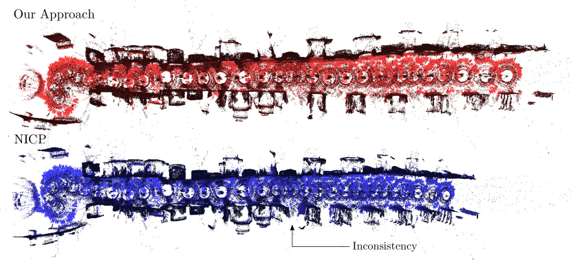
Figure 3: S. Gennaro catacombs dataset, recorded with a RobotEye 3D LIDAR. Direct comparison of our approach with Normal ICP (NICP). The latter shows a registration inconsistency in the middle of the trajectory, with an unexpected change of the orientation around the vertical axis.

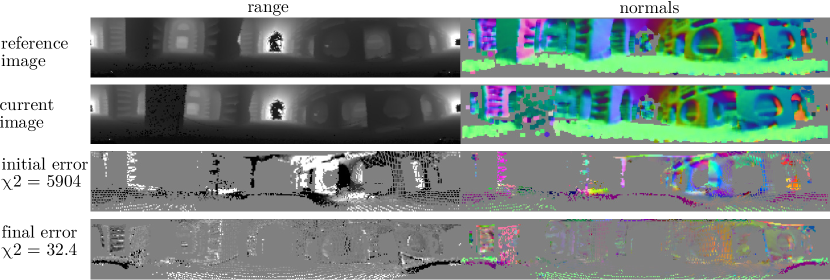
Figure 4: Illustration of the error reduction while registering two images of the S. Gennaro dataset (best viewed on screen).

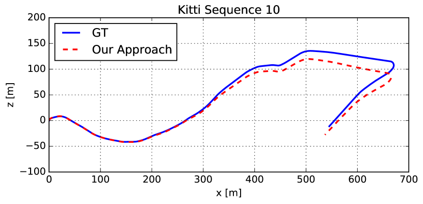
Figure 5: Ground truth comparison in the sequence 10 of the KITTI dataset.

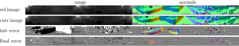
Figure 6: Illustration of the error before and after registering two images of the KITTI dataset. The images are obtained by projecting the Velodyne HDL-64 clouds using a spherical projector (best viewed on screen).

Fig. 3 illustrates the two reconstructions of one of the sequences of the S. Gennaro catacombs, while Fig. 4 shows the error of a pairwise registration before and after the alignment. Thanks to the abstraction provided by the map function and the projective model (see Sec. III-B and III-C), our method can deal with both RGBD data and 3D scans in a uniform manner.

To further stress the generality of our method, we conducted an additional experiment using exactly the same code and parameters using the sequence 10 of the KITTI dataset [4] where we used the 3D scans obtained with a Velodyne HDL-64E LIDAR. As in the previous experiment, the range and normals cues are used. Fig. 6 illustrates the error reduction after the registration of two scans.

As shown in Fig. 5, our output reflects the ground truth with an error of the 7% of the trajectory length, with a rotational error of 0.025 deg/m. Albeit reasonable, this accuracy is still below the one provided by approaches dedicated to the sparse LIDAR such as LOAM [21]. We see the reason of this lower performance in the quantization effects affecting the projections when the clouds are sparse. We plan to address this aspect in future versions by using anisotropic projection functions. Moreover, approaches such as LOAM take advantage from edge and planar surface features, whose usage particularly helps in cases of structure lack.

IV-B Runtime

The next set of experiments is designed to support the last claim, namely that our approach can be executed fast enough to allow for online processing of the sensor data without sensor-specific optimizations. Thus, we report in the remainder of this section the runtime statistics. We performed all the presented experiments on two different computers running Ubuntu 16.04. One is a laptop equipped with a i7-3630MQ CPU with 2.40 GHz and the second one is a desktop computer equipped with a i7-7700K CPU with 4.20 GHz. Our software runs on a single core and in a single thread.

Tab. II summarizes the runtime results for the different configurations presented above. We provide the average results obtained in the four TUM desk sequences for the Kinect RGBD and depth-only configurations, as well as for the two LIDAR setups. As listed in the table, our method can be executed fast and in an online fashion. On a mobile i7 CPU, we achieve average frame rates of 20 Hz with Kinect RGBD sensor and 14 Hz with the Velodyne HDL-64E data, while we achieve average of 30 Hz and 23 Hz on an i7 desktop computer for the same configurations. Furthermore note, that our approach has a small memory footprint. For the whole registration procedure of the three datasets, we always required less than 200 MB (Kinect: 178 MB; RobotEye: 140 MB; HDL-64E: 198 MB).

Note that recording a single RobotEye point clouds takes around 30 s, i.e. the robot stops, records, and then restarts. Thus, this setup may not be considered for real-time usage. In contrast, the Velodyne clouds of the KITTI dataset have been recorded at an average frame rate of 10 Hz and the data can be processed online.

TABLE II: Average image processing runtime with std. deviation

Sensor	laptop computer	desktop computer
	i7-3630MQ 2.4 GHz	i7-7700K 4.2 GHz
Kinect	49 ms $\pm$ 0.8 ms $\approx$ 20.1 Hz	33 ms $\pm$ 0.6 ms $\approx$ 29.8 Hz
RobotEye	324 ms $\pm$ 1.5 ms $\approx$ 3.1 Hz	250 ms $\pm$ 0.8 ms $\approx$ 4 Hz
HDL-64E	67 ms $\pm$ 0.3 ms $\approx$ 14.8 Hz	43 ms $\pm$ 0.1 ms $\approx$ 23.1 Hz

In summary, our evaluation suggests that our method provides competitive results in several different scenarios compared to approaches dedicated to a specific setup. At the same time, our method is fast enough for online processing and has small memory demands, proportional to the number of channels in use. Thus, we conclude that we supported all our four claims made in the introduction.

V Conclusion

In this paper, we presented a general framework for registering sensor data such as RGBD or 3D LIDAR data. Our approach extends dense visual odometry and operates on the different available cues such as color image, depth, and normal information. Our method avoids an explicit data association and operates by direct error minimization using projections of the sensor data or model. This allows us to successfully register data effectively without tricky, sensor-specific adaptations. We implemented and evaluated our approach on different datasets and provided comparisons to other existing techniques and supported all claims made in this paper. The experiments suggest that we can accurately register RGBD and 3D data under realistic configurations and that the computations can be executed at the sensor framerate on a regular notebook computer using a single core.

Appendix A Jacobians

In this section, we focus in more detail on each part of the Jacobian in Eq. (25) and specify all terms used of this equation.

A-A Jacobian of Transformation

We are using the $\mathrm{v2t}(\cdot)$ operator to denote the conversion between $\mathbf{X}$ and $\mathbf{\Delta x}$ as defined in Eq. (6). By applying the $\mathrm{v2t}(\cdot)$ operator, we obtain the standard Jacobian:

$$\mathbf{J}_{\mathrm{tf}}=\frac{\partial\mathrm{v2t}(\mathbf{x})\,\breve{\mathbf{p}}}{\partial\mathbf{x}}\bigg{|}_{\mathbf{x}=0}=\begin{bmatrix}\mathbf{I}&-\breve{\mathbf{p}}_{\times}\end{bmatrix}$$ (26)

where $\mathbf{I}$ is a $3\times 3$ identity matrix and $\breve{\mathbf{p}}_{\times}$ denotes the skew-symmetric matrix formed from $\breve{\mathbf{p}}$.

A-B Map Function Jacobian

The map function Jacobian $\mathbf{J}^{\mathrm{c}}_{\mathrm{map}}$ differs for each of the considered channels $\mathrm{c}$. In this work, we use the following channels: intensity, depth, range and normals. In the following we present the Jacobian derivation of each of these cues.

Intensity: The map function does not affect the intensity, thus we have:

$$\frac{\partial\mathrm{map}^{\mathrm{intensity}}(\mathbf{X}\oplus\mathbf{x},\mathbf{p})}{\partial\mathbf{x}}\bigg{|}_{\mathbf{x}=0}=0$$ (27)

Depth: We have already computed the derivative of the transformation function $\mathbf{J}_{\mathrm{tf}}$ in Eq. (26). For RGBD sensors, the depth is computed as the $z$ coordinate of the transformed point $\mathbf{p}$. Thus, the map Jacobian for the depth channel is the third row of $\mathbf{J}_{\mathrm{tf}}$

$$\frac{\partial\mathrm{map}^{0pt}(\mathbf{X}\oplus\mathbf{x},\mathbf{p})}{\partial\mathbf{x}}\bigg{|}_{\mathbf{x}=0}=\begin{bmatrix}0&0&1\end{bmatrix}\cdot\mathbf{J}_{\mathrm{tf}}$$ (28)

Range: When using a 3D LIDAR, the range $r=\|\mathbf{p}\|$ replaces the depth. Thus, the Jacobian $\mathbf{J}_{\mathrm{map}}^{\mathrm{range}}$ is computed as

$$\mathbf{J}_{\mathrm{map}}^{\mathrm{range}} = \frac{\partial\mathrm{map}^{\mathrm{range}}(\mathbf{X}\oplus\mathbf{x},\mathbf{p})}{\partial\mathbf{x}}\bigg{|}_{\mathbf{x}=0}$$ (29)

$$= \frac{\partial\mathrm{range}(\mathrm{v2t}(\mathbf{x})\,\mathbf{X}\mathbf{p})}{\partial\mathbf{x}}\bigg{|}_{\mathbf{x}=0}$$

$$= \frac{\partial\mathrm{range}(\breve{\mathbf{p}})}{\partial\breve{\mathbf{p}}}\bigg{|}_{\breve{\mathbf{p}}=\mathbf{X}\mathbf{p}}\,\frac{\partial\mathrm{v2t}(\mathbf{x})\,\mathbf{X}\mathbf{p}}{\partial\mathbf{x}}\bigg{|}_{\mathbf{x}=0}$$

$$= \frac{\partial\mathrm{range}(\breve{\mathbf{p}})}{\partial\breve{\mathbf{p}}}\bigg{|}_{\breve{\mathbf{p}}=\mathbf{X}\mathbf{p}}\,\mathbf{J}_{\mathrm{tf}}$$

$$= \frac{1}{\mathrm{norm}(\mathbf{p})}\begin{bmatrix}\mathbf{p}_{x}&\mathbf{p}_{y}&\mathbf{p}_{z}\end{bmatrix}\cdot\mathbf{J}_{\mathrm{tf}}$$

Normals: The mapping function applied to the normals cue depends on the rotational part of $\mathbf{X}$ and the Jacobian is given by

$$\frac{\partial\mathrm{map}^{\mathrm{normal}}(\mathbf{X}\oplus\mathbf{x},\mathbf{p})}{\partial\mathbf{x}}\bigg{|}_{\mathbf{x}=0}=\begin{bmatrix}\mathbf{0}&-{[\mathbf{R}\,\mathbf{n}(\mathbf{p})]}_{\times}\end{bmatrix},$$ (30)

where $\mathbf{R}$ denotes a rotation matrix, $\mathbf{n}(\mathbf{p})$ the normal defined for the point $\mathbf{p}$, and ${[\mathbf{R}\,\mathbf{n}(\mathbf{p})]}_{\times}$ the skew-symmetric matrix.

A-C Image Jacobian

The Image Jacobian $\mathbf{J}^{\mathrm{c}}_{\mathrm{img}}$ is numerically computed for each channel $\mathrm{c}$ with pixel-wise derivation:

$$\frac{\partial\boldsymbol{\mathfrak{I}}^{\mathrm{c}}_{u,v}}{\partial u} = \frac{1}{2}\left(\boldsymbol{\mathfrak{I}}^{\mathrm{c}}_{u+1,v}-\boldsymbol{\mathfrak{I}}^{\mathrm{c}}_{u-1,v}\right)$$

$$\frac{\partial\boldsymbol{\mathfrak{I}}^{\mathrm{c}}_{u,v}}{\partial v} = \frac{1}{2}\left(\boldsymbol{\mathfrak{I}}^{\mathrm{c}}_{u,v+1}-\boldsymbol{\mathfrak{I}}^{\mathrm{c}}_{u,v-1}\right)$$ (31)

A-D Jacobian of Projection

The Jacobian of the projection depends directly on the projection function $\mathbf{J}_{\mathrm{proj}}=\frac{\partial\mathrm{proj}(\mathbf{p})}{\partial\mathbf{p}}$. In the following, we provide details for the two models given in Sec. III-C.

Pinhole Model: We derive the projection Jacobian for a pinhole camera from Eq. (22):

$$\frac{\partial\mathrm{proj}(\mathbf{p})}{\partial\mathbf{p}} = \frac{\partial\pi(\mathbf{p}^{\prime})}{\partial\mathbf{p}^{\prime}}\bigg{|}_{\mathbf{p}^{\prime}=\mathbf{K}\,\mathbf{p}}\,\frac{\partial\mathbf{K}\,\mathbf{p}}{\partial\mathbf{p}}$$

$$= \frac{1}{z^{2}}\begin{bmatrix}z&0&-x\\ 0&z&-y\end{bmatrix}\bigg{|}_{(x,y,z)=\mathbf{K}\,\mathbf{p}}\,\mathbf{K}$$

Spherical Model: The projection function for the range sensors is defined in Eq. (23). We make use of the substitution $\mathbf{a}_{2}=\sqrt{\mathbf{p}_{x}^{2}+\mathbf{p}_{y}^{2}}$, and define the Jacobian as follows:

$$\frac{\partial\mathrm{proj}(\mathbf{p})}{\partial\mathbf{p}}=\begin{bmatrix}\frac{1}{\mathbf{a}_{2}^{2}}\,\begin{bmatrix}-\mathbf{p}_{y}&\mathbf{p}_{x}&0\end{bmatrix}\\ \frac{1}{\mathbf{a}_{2}^{2}+\mathbf{p}_{z}^{2}}\,\begin{bmatrix}-\frac{\mathbf{p}_{x}\,\mathbf{p}_{z}}{\mathbf{a}_{2}}&-\frac{\mathbf{p}_{y}\,\mathbf{p}_{z}}{\mathbf{a}_{2}}&\mathbf{a}_{2}\end{bmatrix}\\ \begin{bmatrix}0&0&0\end{bmatrix}\end{bmatrix}\,\mathbf{K}$$ (33)

References

- [1] M. Bloesch, S. Omari, M. Hutter, and R. Siegwart. Robust visual inertial odometry using a direct ekf-based approach. In Proc. of the IEEE/RSJ Intl. Conf. on Intelligent Robots and Systems (IROS), pages 298–304, Sept 2015.
- [2] J. Engel, T. Schöps, and D. Cremers. Lsd-slam: Large-scale direct monocular slam. In Proc. of the Europ. Conf. on Computer Vision (ECCV), pages 834–849. Springer, Cham, 2014.
- [3] C. Forster, Z. Zhang, M. Gassner, M. Werlberger, and D. Scaramuzza. Svo: Semidirect visual odometry for monocular and multicamera systems. IEEE Trans. on Robotics (TRO), 33(2):249–265, April 2017.
- [4] A. Geiger, P. Lenz, and R. Urtasun. Are we ready for autonomous driving? the kitti vision benchmark suite. In Proc. of the IEEE Conf. on Computer Vision and Pattern Recognition (CVPR), 2012.
- [5] M. Jaimez and J. Gonzalez-Jimenez. Fast visual odometry for 3-d range sensors. IEEE Trans. on Robotics (TRO), 31(4):809–822, Aug 2015.
- [6] M. Keller, D. Lefloch, M. Lambers, and S. Izadi. Real-time 3D Reconstruction in Dynamic Scenes using Point-based Fusion. In Proc. of the International Conference on 3D Vision (3DV), pages 1–8, 2013.
- [7] C. Kerl, J. Stuckler, and D. Cremers. Dense continuous-time tracking and mapping with rolling shutter rgb-d cameras. In Proc. of the IEEE Intl. Conf. on Computer Vision (ICCV), pages 2264–2272, 2015.
- [8] C. Kerl, J. Sturm, and D. Cremers. Dense visual slam for rgb-d cameras. In Proc. of the IEEE/RSJ Intl. Conf. on Intelligent Robots and Systems (IROS), pages 2100–2106. IEEE, 2013.
- [9] C. Kerl, J. Sturm, and D. Cremers. Robust odometry estimation for rgb-d cameras. In Proc. of the IEEE Intl. Conf. on Robotics & Automation (ICRA), pages 3748–3754. IEEE, 2013.
- [10] R. A. Newcombe, S. Izadi, O. Hilliges, D. Molyneaux, D. Kim, A. J. Davison, P. Kohli, J. Shotton, S. Hodges, and A. Fitzgibbon. KinectFusion: Real-Time Dense Surface Mapping and Tracking. In Proc. of the Intl. Symposium on Mixed and Augmented Reality (ISMAR), pages 127–136, 2011.
- [11] D. Nister, O. Naroditsky, and J. Bergen. Visual odometry. In Proc. of the IEEE Conf. on Computer Vision and Pattern Recognition (CVPR), volume 1, pages I–652–I–659 Vol.1, June 2004.
- [12] A. Segal, D. Haehnel, and S. Thrun. Generalized-icp. In Proc. of Robotics: Science and Systems (RSS), volume 2, 2009.
- [13] J. Serafin, M. Di Cicco, T. M. Bonanni, G. Grisetti, L. Iocchi, D. Nardi, C. Stachniss, and V. A. Ziparo. Robots for exploration, digital preservation and visualization of archeological sites. In Artificial Intelligence for Cultural Heritage, chapter 5, pages 121–140. 2016.
- [14] J. Serafin and G. Grisetti. NICP: Dense Normal Based Point Cloud Registration. In Proc. of the IEEE/RSJ Intl. Conf. on Intelligent Robots and Systems (IROS), pages 742–749, 2015.
- [15] J. Serafin and G. Grisetti. Using extended measurements and scene merging for efficient and robust point cloud registration. Journal on Robotics and Autonomous Systems (RAS), 92(C):91–106, June 2017.
- [16] M. Slavcheva, W. Kehl, N. Navab, and S. Ilic. Sdf-2-sdf: Highly accurate 3d object reconstruction. In Proc. of the Europ. Conf. on Computer Vision (ECCV), pages 680–696. Springer International Publishing, 2016.
- [17] J. Sturm, N. Engelhard, F. Endres, W. Burgard, and D. Cremers. A benchmark for the evaluation of rgb-d slam systems. In Proc. of the IEEE/RSJ Intl. Conf. on Intelligent Robots and Systems (IROS), Oct. 2012.
- [18] T. Weise, T. Wismer, B. Leibe, and L. Van Gool. Online loop closure for real-time interactive 3D scanning. Journal of Computer Vision and Image Understanding (CVIU), 115:635–648, 2011.
- [19] J. Yang, H. Li, D. Campbell, and Y. Jia. Go-icp: A globally optimal solution to 3d icp point-set registration. IEEE Trans. on Pattern Analalysis and Machine Intelligence (TPAMI), 38(11):2241–2254, Nov 2016.
- [20] J. Zhang and S. Singh. LOAM: Lidar Odometry and Mapping in Real-time. In Proc. of Robotics: Science and Systems (RSS), 2013.
- [21] J. Zhang and S. Singh. Low-drift and real-time lidar odometry and mapping. Autonomous Robots, pages 1–16, 2016.
- [22] X. Zheng, Z. Moratto, M. Li, and A. Mourikis. Photometric Patch-Based Visual-Inertial Odometry. In Proc. of the IEEE Intl. Conf. on Robotics & Automation (ICRA), 2017.