Light propagation in linearly perturbed $\Lambda$LTB models

Abstract

We apply a generic formalism of light propagation to linearly perturbed spherically symmetric dust models including a cosmological constant. For a comoving observer on the central worldline, we derive the equation of geodesic deviation and perform a suitable spherical harmonic decomposition. This allows to map the abstract gauge-invariant perturbation variables to well-known quantities from weak gravitational lensing like convergence or cosmic shear. The resulting set of differential equations can effectively be solved by a Green’s function approach leading to line-of-sight integrals sourced by the perturbation variables on the backward lightcone. The resulting spherical harmonic coefficients of the lensing observables are presented and the shear field is decomposed into its E- and B-modes. Results of this work are an essential tool to add information from linear structure formation to the analysis of spherically symmetric dust models with the purpose of testing the Copernican Principle with multiple cosmological probes.

1 Introduction

Exact cosmological solutions of general relativity (GR) have become an important tool to test the foundations of the standard cosmological model. These particular models are based on the class of spatially homogeneous and isotropic Friedmann-Lemaître-Robertson-Walker (FLRW) models and turned out to be remarkably successful in describing multiple observational probes on a huge variety of time- and spatial scales (see for example [1] for a review). Despite this success, its foundations need to be tested in a best possible, complete and consistent way. One possible approach focusses on the construction of more general exact solutions of GR and deriving possible observational implications. One of the simplest possible generalisations of the FLRW class is the $\Lambda$-Lemaître-Tolman-Bondi ($\Lambda$LTB) spacetime (see [2], [3], and [4]) that can be foliated into spatial hypersurfaces that are spherically symmetric about one distinct central worldline. The corresponding degree of freedom of a radial density and curvature profile of the universe allows to model the possible deviations from spatial homogeneity that would break the Copernican Principle. For extensive reviews on the properties of ($\Lambda$)LTB solutions we refer to ([5, 6, 7, 8]). It is important to constrain these deviations with best significance including as many as possible of the cosmological observables available. Cosmological models based on the $\Lambda$LTB solution have been constrained by multiple observational probes and so far no significant deviation from spatial homogeneity has been found (see [8, 9]). However, up to very few exceptions based on simplifying assumptions (see [10, 11]), a fully consistent inclusion of information from linear structure formation is still missing which excludes several important cosmological probes like cosmic shear or the integrated Sachs-Wolfe effect.

Linear perturbation theory in radially inhomogeneous solutions are substantially more complicated than in standard FLRW models. The reduced degree of symmetry causes the dynamical evolution of gauge-invariant linear perturbations to be described by partial differential equations that contain a complicated dynamical coupling. The full evolution equations have first been derived in [12] while first numerical investigations were performed in [13, 14]. However, the structure of these gauge-invariant quantities is non-trivial as they reduce to complicated mixings of FLRW scalar-vector-tensor variables in the limit of spatial homogeneity (see [12] for the first detailed analysis of this issue). This means that, although the dynamics of gauge-invariant, physical perturbation variables in $\Lambda$LTB cosmologies can be modeled numerically, the results cannot be interpreted physically in a straightforward way.

In this context, light propagation in $\Lambda$LTB models is a promising approach to study observational effects of gauge-invariant perturbative quantities on these radially inhomogeneous backgrounds. In fact, combined influences of metric and matter perturbations on null geodesics can be mapped to corrections to the angular diameter distance that itself can be converted to observables extracted from weak gravitational lensing. This work aims at constructing the necessary expressions connecting light propagation equations to the combined effect of gauge-invariant metric and fluid perturbations. It therefore provides the foundations to include observables from linear structure formation into a most complete analysis of $\Lambda$LTB models.

The paper is structured as follows: Sect. (2) outlines a generic and well-known relativistic approach to light propagation starting with thin bundles of null geodesics. A short summary on the geodesic deviation equation in $\Lambda$LTB models is provided in Sect. (3). In the following Sect. (4), we derive the full equation system for geodesic deviation in linearly perturbed $\Lambda$LTB models which is decomposed into spherical harmonics functions. In Sect. (5) we address a possible solution based on a Green’s function approach yielding line-of-sight integral expressions for the lensing observables. The resulting cosmic shear field will then be split into the E- and B-modes in Sect. (6).

2 Light propagation in general relativity

The following section provides a short summary on relativistic light propagation as well as the conventions and notation applied in this work. It is mainly based on the approaches presented in [15, 16]. We consider an infinitesimal bundle of null geodesics (see [17] for an exact definition) that is propagating in an arbitrary spacetime and converges at an observer freely falling with four-velocity $u_{\mathrm{obs}}$. One particular geodesic of the bundle can be singled out as a so-called fiducial ray and parametrised by an affine parameter $\lambda$. Given the observer’s local coordinates $x^{\mu}$, we define the ray’s wave vector as

$$k^{\mu}=\frac{\mathrm{d}x^{\mu}}{\mathrm{d}\lambda}$$ (2.1)

and choose $\lambda$ such that a unit projection of $k$ on $u_{\mathrm{obs}}$ is obtained. Effectively, this corresponds to a normalisation of the wave vector by the observed frequency of the light ray. Starting from

$$\langle k,u_{\mathrm{obs}}\rangle=-\omega_{\mathrm{obs}}\,,$$ (2.2)

we transform $k^{\mu}\longrightarrow\tilde{k}^{\mu}=-k^{\mu}/\omega_{\mathrm{obs}}\equiv k^{\mu}$ such that

$$\langle k,u_{\mathrm{obs}}\rangle=1\,.$$ (2.3)

Given this affine parametrisation, $\lambda$ corresponds to the Euclidian distance in the local neighborhood of the freely falling observer $\mathrm{d}\lambda=\mathrm{d}r$. In addition, the redshift of a fictitious source with respect to the observer can be defined as

$$\langle k,u_{\mathrm{s}}\rangle=1+z\,,$$ (2.4)

where $u_{\mathrm{s}}$ denotes the source’s four-velocity. The redshift is normalised to zero for a comoving source placed at the observer’s position.

We now consider the spacelike plane perpendicular to $k$ and $u_{\mathrm{obs}}$ which defines a screen in the rest frame of the observer. An orthonormal basis of this screen is generally given by the two vectors $n^{\mu}_{\ a}$ $(a=1,2)$ which are commonly referred to as Sachs basis. By construction, the Sachs basis vectors then fulfill the following identities:

$$k_{\mu}{n^{\mu}}_{a} =0\,,$$ (2.5)

$$u_{\mu}{n^{\mu}}_{a} =0\,,$$ (2.6)

$$n_{\mu,a\vphantom{b}}{n^{\mu}}_{b} =\delta_{ab}\,.$$ (2.7)

Having set-up the Sachs basis at $\lambda=0$, the basis vectors at arbitrary affine parameters can be obtained by parallel transport ($\nabla_{k}n_{a}=0$) of the initial basis along the fiducial ray. Given the Riemannian connection, Eqs. (2.5) - (2.7) are not affected by this procedure.

A general vector in the screen space can be constructed by defining a second affine parameter $\sigma$ and a corresponding spacelike curve $\gamma(\sigma)$ that connects the fiducial ray with neighboring geodesics (see Fig. (1)). By assumption, $\gamma(\sigma)$ is entirely contained in the screen space such that the tangent vector

$$\eta^{\mu}=\left.\frac{\mathrm{d}\gamma^{\mu}}{\mathrm{d}\sigma}\right|_{\sigma=0}$$ (2.8)

can be expanded into the Sachs basis vectors

$$\eta^{\mu}=\eta_{1}{n^{\mu}}_{1}+\eta_{2}{n^{\mu}}_{2}\,.$$ (2.9)

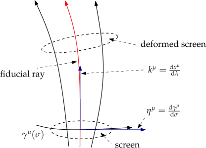
Figure 1: Construction of a screen space for a bundle of null geodesics: The evolution of the geodesic bundle can be mapped to the corresponding deformation of the screen when parallel-transported along the fiducial ray.

For a proper choice of the affine parameter $\sigma$, $\eta^{\mu}$ measures the physical size and shape of the bundle when parallel-transported along the fiducial ray. The evolution of $\eta^{\mu}$ is given by the equation of geodesic deviation

$$k^{\alpha}k^{\beta}\nabla_{\alpha}\nabla_{\beta}\eta^{\mu}=R^{\mu}_{\ \nu\alpha\beta}k^{\nu}k^{\alpha}\eta^{\beta}\,,$$ (2.10)

containing the generic Riemann tensor of the spacetime.

Inserting Eq. (2.9) into Eq. (2.10), we obtain

$$\frac{\mathrm{d}^{2}\eta_{a}}{\mathrm{d}\lambda^{2}}=R_{\mu\nu\alpha\beta}{n^{\mu}}_{a}k^{\nu}k^{\alpha}{n^{\beta}}_{b}\eta_{b}=\mathcal{T}_{ab}\eta_{b}\,,$$ (2.11)

where summation over $b$ is implied. The object $\mathcal{T}_{ab}$ is the so-called optical tidal matrix as it connects the evolution of the geodesic bundle with the curvature of spacetime. It separates into two distinct contributions

$$\mathcal{T}_{ab}=-\frac{1}{2}R_{\alpha\beta}k^{\alpha}k^{\beta}\delta_{ab}+C_{\mu\nu\alpha\beta}{n^{\mu}}_{a}k^{\nu}k^{\alpha}{n^{\beta}}_{b}\,,$$ (2.12)

which define the so-called Ricci- and Weyl focussing terms. The Ricci focussing originates from matter inside the bundle that causes $\eta^{\mu}$ to increase or decrease isotropically. On the other hand, the Weyl focussing is generated by matter located outside the bundle giving rise to shear effects on the screen. The role of the two different contributions will be discussed below in more detail.

Since Eq. (2.11) is a second order ordinary differential equation in the affine parameter $\lambda$, any solution is constrained by two initial conditions given by the initial value and the initial first derivative of $\eta^{\mu}$. As assumed a priori, the bundle converges at the freely falling observer placed at $\lambda=0$ which fixes $\eta^{\mu}(\lambda=0)$ to zero. The final solution can therefore only depend on the initial rate $\left.\mathrm{d}\eta^{\mu}/\mathrm{d}\lambda\right|_{\lambda=0}$. In case of a linear differential equation, the solution this yields the mapping

$$\eta_{a}(\lambda)=\left.D_{ab}(\lambda)\frac{\mathrm{d}\eta_{b}}{\mathrm{d}\lambda}\right|_{\lambda=0}\,,$$ (2.13)

with the Jacobi map $D_{ab}$ that contains all information on the evolution of the geodesic bundle with respect to $\lambda$. Hence, the full initial value problem can be formulated in terms of the Jacobi map which yields Jacobi matrix equation:

$$\begin{split}\frac{\mathrm{d}^{2}D_{ab}}{\mathrm{d}\lambda^{2}}\quad&=\mathcal{T}_{ac\vphantom{b}}D_{cb}\,,\\ \left.D_{ab}\right|_{\lambda=0}&=0\,,\\ \left.\frac{\mathrm{d}D_{ab}}{\mathrm{d}\lambda}\right|_{\lambda=0}&=\delta_{ab}\,,\end{split}$$ (2.14)

which is independent of the initial rate of $\eta_{a}$. We have chosen the affine parameter $\lambda$ to coincide with the local Euclidian distance in the observer’s rest frame. Thus, the initial rate can locally be interpreted as the opening angle

$$\theta_{a}=\left.\frac{\mathrm{d}\eta_{a}}{\mathrm{d}\lambda}\right|_{\lambda=0}$$ (2.15)

in this particular frame. Integrating Eq. (2.14) from the observer to a fiducial source located at a position corresponding to the affine parameter $\lambda_{s}$ leads to

$$\eta_{a}(\lambda_{s})=D_{ab}(\lambda_{s})\left.\frac{\mathrm{d}\eta_{b}}{\mathrm{d}\lambda}\right|_{\lambda=0}=D_{ab}(\lambda_{s})\theta_{b}\,.$$ (2.16)

This means that the Jacobi map relates cross-sectional diameters of the bundle at the source position to angular diameters at the observer which defines an angular diameter distance. Precisely, this definition only holds for infinitesimal bundles with circular cross section. In case of general elliptical cross sections, $D_{ab}$ can be diagonalised yielding two extremal angular diameter distances $D_{+}(\lambda_{s})$ and $D_{-}(\lambda_{s})$. In fact, a circular image of angular size $\theta$ seen by an observer has an elliptical cross-section with principal axes $|D_{\pm}(\lambda_{s})|\cdot\theta$ at the source position (see [17] for details). Therefore, the angular diameter distance shall be replaced by the so-called area distance that relates the cross-sectional area of the bundle at the source position to the solid angle seen by the observer. Involving the geometric interpretation of the determinant, the area distance can be defined as (see [16, 17])

$$D_{A}(\lambda_{s})=\sqrt{(\det{D_{ab}})(\lambda_{s})}=\sqrt{D_{+}(\lambda_{s})D_{-}(\lambda_{s})}\,.$$ (2.17)

Due to its general applicability, this definition will be considered as angular diameter distance in the following. $D_{A}$ is an important physical quantity as it can directly be inferred from observations. Once a physical length scale of a particular source is known, the opening angle can be measured and $D_{A}$ readily estimated. On the other hand, $D_{A}$ is related to the Jacobi map which is itself a solution to the Jacobi matrix equation. It is therefore sensitive to the spacetime geometry due to the Weyl and Ricci focussing terms in the optical tidal matrix. Effects of gauge-invariant perturbations of the background spacetime can therefore be mapped to physically meaningful observables. This is a most welcome property in case of more abstract gauge-invariants such as those appearing in gauge-invariant $\Lambda$LTB perturbation theory.

The Jacobi map can be related to the Jacobian matrix $A_{ab}$ of the lens mapping (see [15]) which is also denoted as lensing amplification matrix. We recover again Eq. (2.15) since it defines the angle under which a source is seen at the observer’s position. The angular position $\beta_{a}$ of the source without focussing effects is given by

$$\beta_{a}=\frac{\eta_{a}(\lambda_{s})}{\mkern 1.5mu\overline{\mkern-1.5muD\mkern-1.5mu}\mkern 1.5mu_{A}(\lambda_{s})}\,,$$ (2.18)

where $\mkern 1.5mu\overline{\mkern-1.5muD\mkern-1.5mu}\mkern 1.5mu_{A}(\lambda_{s})$ is the area angular diameter distance of a background spacetime in which focussing effects due to perturbations are studied. When combining Eqs. (2.15) and (2.17), we obtain the lens map that relates the angular position of the source to the observed angular position due to focussing effects:

$$\beta_{a}=\frac{\eta_{a}(\lambda_{s})}{\mkern 1.5mu\overline{\mkern-1.5muD\mkern-1.5mu}\mkern 1.5mu_{A}(\lambda_{s})}=\frac{D_{ab}(\lambda_{s})}{\mkern 1.5mu\overline{\mkern-1.5muD\mkern-1.5mu}\mkern 1.5mu_{A}(\lambda_{s})}\theta_{b}=A_{ab}(\lambda_{s})\theta_{b}.$$ (2.19)

Hence, the lensing amplification matrix is generally expressed as

$$A_{ab}(\lambda)=\frac{D_{ab}(\lambda)}{\mkern 1.5mu\overline{\mkern-1.5muD\mkern-1.5mu}\mkern 1.5mu_{A}(\lambda)}\,,$$ (2.20)

which can conveniently be decomposed into a trace and trace-free part

$$(A_{ab})=\left(\begin{array}[]{cc}1-\kappa&0\\ 0&1-\kappa\end{array}\right)-\left(\begin{array}[]{cc}\gamma_{1}&\gamma_{2}\\ \gamma_{2}&-\gamma_{1}\end{array}\right)\,.$$ (2.21)

3 Geodesic deviation in $\Lambda$LTB cosmologies

The concepts introduced in the previous section can now readily be applied to $\Lambda$LTB models. The $\Lambda$LTB solution is a dust solution of Einstein’s field equations with hypersurfaces that are spherically symmetric about one central worldline. The line element in comoving synchronous coordinates (see [18]) reads

$$\mathrm{d}s^{2}=-\mathrm{d}t^{2}+\frac{a_{\|}^{2}(t,r)}{1-\kappa(r)r^{2}}\mathrm{d}r^{2}+r^{2}a_{\perp}^{2}(t,r)\mathrm{d}\Omega^{2}\,,$$ (3.1)

with an energy momentum tensor $T_{\mu\nu}=\rho(t,r)u_{\mu}u_{\nu}$. Inward radial null geodesics for a central observer are constrained by the following equation system

$$\frac{\mathrm{d}t(r)}{\mathrm{d}r} =-\frac{a_{\|}(t(r),r)}{\sqrt{1-\kappa(r)r^{2}}}\,,$$ (3.2)

$$\frac{1}{1+z(r)}\frac{\mathrm{d}z(r)}{\mathrm{d}r} =\frac{\dot{a}_{\|}(t(r),r)}{\sqrt{1-\kappa(r)r^{2}}}\,,$$ (3.3)

Throughout this work, we will restrict ourselves to observers located at the center of a $\Lambda$LTB patch, because this yields a considerable simplification of the expressions derived in the next section. However, conceptually there is no restriction of the observer’s position to the center. Off-center observers in LTB void models at the background level have been considered in previous works (see [19], [20] as well as [21]). In this context, geodesic lightcone coordinates (see [22]) have proven to be very effective, but this approach will not be followed in this work .

Using Eqs. (3.2), (3.3), and (2.1), differential relations between the affine parameter $\lambda$ and coordinate time, radius, and redshift can be derived

$$\frac{\mathrm{d}t(\lambda)}{\mathrm{d}\lambda} =-(1+z(\lambda))\,,$$ (3.4)

$$\frac{\mathrm{d}r(\lambda)}{\mathrm{d}\lambda} =(1+z(\lambda))\,\frac{\sqrt{1-\kappa(r(\lambda))r^{2}(\lambda)}}{a_{\|}(t(\lambda),r(\lambda))}\,,$$ (3.5)

$$\frac{\mathrm{d}z(\lambda)}{\mathrm{d}\lambda} =(1+z(\lambda))^{2}H_{\|}(t(\lambda),r(\lambda))\,,$$ (3.6)

which form a coupled system of ordinary differential equations constraining the shape of the background $\Lambda$LTB past null cone.

As the $\Lambda$LTB solution is spherically symmetric about the central worldline, the Weyl focussing term in the optical tidal matrix vanishes and the field equations constrain the Ricci focussing term to be

$$\begin{split}\mathcal{T}_{ab}&=-\frac{1}{2}R_{\alpha\beta}k^{\alpha}k^{\beta}\delta_{ab}=-\frac{1}{2}T_{\alpha\beta}k^{\alpha}k^{\beta}\delta_{ab}\\ &=-4\pi G\rho(t,r)\,(1+z)^{2}\delta_{ab}\,.\end{split}$$ (3.7)

The geodesic deviation equation then reads

$$\frac{\mathrm{d}^{2}D_{ab}(\lambda)}{\mathrm{d}\lambda^{2}}=-4\pi G\rho(t(\lambda),r(\lambda))\,(1+z(\lambda))^{2}D_{ab}(\lambda)\,,$$ (3.8)

which has to be solved in combination with Eqs. (3.4)-(3.6) using the initial conditions

$$\begin{split}\left.D_{ab}\right|_{\lambda=0}&=0\,,\\ \left.\frac{\mathrm{d}D_{ab}}{\mathrm{d}\lambda}\right|_{\lambda=0}&=\delta_{ab}\,,\end{split}$$

$$\left.t\right|_{\lambda=0} =t_{\mathrm{age}}\,,$$

$$\left.r\right|_{\lambda=0} =0\,,$$

$$\left.z\right|_{\lambda=0} =0\,.$$

In general, this system has to be evolved numerically, but there exists an analytic solution to Eq. (3.8) without knowledge of the exact shape of the backward lightcone. By taking Eqs. (3.4)-(3.6) as differential relations and involving the field equations at the background level (see also Appendix (A)), it can be shown that

$$D_{ab}(\lambda)=r(\lambda)a_{\perp}(t(\lambda),r(\lambda))\delta_{ab}$$ (3.9)

solves Eq. (3.8). This result which has also previously been found in ([11]) is physically meaningful as it describes the areal radius of the line element (Eq. (3.8)) fixing the angular diameter distance for a central observer. Eq. (3.9) turns out to be very useful in the following sections.

4 Geodesic deviation in perturbed $\Lambda$LTB cosmologies

As proposed in ([24]), a 2+2 split of the full spacetime $\mathcal{M}^{4}=\mathcal{M}^{2}\times\mathcal{S}^{2}$ leads to gauge-invariant linear perturbations that can be expressed in terms of scalar, vector and tensor spherical harmonics. Those naturally split into an even, polar and an odd, axial branch by considering their curl-free and divergence-free parts on $\mathcal{S}^{2}$, respectively. In the polar branch, there are four degrees of freedom $\chi^{(\ell m)}$, $\varphi^{(\ell m)}$, $\varsigma^{(\ell m)}$, and $\eta^{(\ell m)}$ entering the linearly perturbed metric as well as three expressions $\Delta^{(\ell m)}$, $w^{(\ell m)}$, and $v^{(\ell m)}$ fixing the energy-momentum tensor (see [12]). In Regge-Wheeler (RW) gauge (see [25]), the perturbed metric and energy-momentum tensor read:

$$ds^{2} =-\left[1+(2\eta^{(\ell m)}-\chi^{(\ell m)}-\varphi^{(\ell m)})Y^{(\ell m)}\right]\mathrm{d}t^{2}-\frac{2a_{\|}\varsigma^{(\ell m)}Y^{(\ell m)}}{\sqrt{1-\kappa r^{2}}}\mathrm{d}t\mathrm{d}r$$ (4.1)

$$\ \ \ \ +\frac{a_{\|}^{2}}{1-\kappa r^{2}}\left[1+(\chi^{(\ell m)}+\varphi^{(\ell m)})Y^{(\ell m)}\right]\mathrm{d}r^{2}+r^{2}a_{\perp}^{2}\left[1+\varphi^{(\ell m)}Y^{(\ell m)}\right]\mathrm{d}\Omega^{2}\,,$$

$$\rho =\rho^{\mathrm{LTB}}\left(1+\Delta^{(\ell m)}Y^{(\ell m)}\right)\,,$$ (4.2)

$$u_{\mu} =\left[u_{A}+\left(w^{(\ell m)}n_{A}+\frac{1}{2}k_{AB}u^{B}\right)Y^{(\ell m)},v^{(\ell m)}Y_{b}^{(\ell m)}\right]\,,$$ (4.3)

with sums over $(\ell,m)$ implied and $Y_{b}^{(\ell m)}=\nabla_{b}Y^{(\ell m)}$. The unit vectors in time and radial directions are given by $u_{A}=(-1,0)$ and $n_{A}=(0,a_{\|}/\sqrt{1-\kappa r^{2}})$. $k_{AB}$ corresponds to the metric perturbation in the $(t,r)$-submanifold.

The gauge-invariant perturbations of the axial branch consist of a vector field $k_{A}$ and scalar $\mkern 1.5mu\overline{\mkern-1.5muv\mkern-1.5mu}\mkern 1.5mu^{(\ell m)}$:

$$\mathrm{d}s^{2}=-\mathrm{d}t^{2}+\frac{a_{\|}(t,r)^{2}}{1-\kappa(r)r^{2}}\mathrm{d}r^{2}+r^{2}a_{\perp}^{2}(t,r)\mathrm{d}\Omega^{2}+2k_{A}\mathrm{d}x^{A}\bar{Y}^{(\ell m)}_{b}\mathrm{d}x^{b}\,,$$ (4.4)

and

$$u_{\mu}=\left(u_{A},\bar{v}\bar{Y}^{(\ell m)}_{a}\right)\,.$$ (4.5)

We arrive at six degrees of freedom in total for the metric and four degrees of freedom for the energy-momentum tensor. Einstein’s field equations constrain the dynamical evolution of these equations for the polar and axial branch. Whereas both branches are dynamically decoupled, this does not hold for the gauge-invariant quantities in each branch due to the reduced degree of symmetry of the $\Lambda$LTB solution with respect to FLRW models. This also leads to a complicated structure of these quantities in the limit of spatial homogeneity as they mix FLRW scalar-vector-tensor degrees of freedom. For details on the evolution equations and construction of gauge-invariant quantities we refer to ([12]). First numerical investigations on the evolution of gauge-invariant quantities can be found in ([13]) and ([14]).

Generically perturbed $\Lambda$LTB spacetimes do not obey any symmetries seen by observers moving on the $\Lambda$LTB central worldline. Strictly speaking, even this special position in spacetime cannot be precisely singled out anymore. However, assuming that deviations from the spherically symmetric $\Lambda$LTB solution are small, the following approximations can be made:

• The observer’s worldline is approximated by a geodesic in the background LTB spacetime. Hence, the observer’s rest frame and the corresponding central worldline can be described by the $\Lambda$LTB background expressions only.

• Born’s approximation can be applied where influences of perturbations on the propagation of null geodesics are integrated along the unperturbed lightpath. Since metric potentials are assumed to be small, this approximation is typically very accurate (see [26, 27]).

Referring to these approximations, perturbations of the wave vector $k^{\mu}$ and the Sachs basis $n^{\mu}_{\ a}$ as well as deviations in the affine parameter $\lambda$, redshift, and lightcone coordinates from their background values are not considered. This allows to adopt Eqs. (3.4) - (3.6) right away from the background model and consider only perturbations in the optical tidal matrix.

Since we deal with a spherically symmetric solution around a central observer, it is convenient to adapt the Sachs basis of the screen to a spherical basis by demanding

$$n_{\mu,a\vphantom{b}}{n^{\mu}}_{b} =\gamma_{ab}\,.$$ (4.6)

with $(\gamma_{ab})$ denoting the metric on $\mathcal{S}^{2}$.

The optical tidal matrix in this screen basis then reads

$$\mathcal{T}_{ab}=-\frac{1}{2}R_{\alpha\beta}k^{\alpha}k^{\beta}\gamma_{ab}+C_{\mu\nu\alpha\beta}{n^{\mu}}_{a}k^{\nu}k^{\alpha}{n^{\beta}}_{b}\,.$$ (4.7)

The Jacobi matrix can be split into a background contribution $D^{(0)}_{ab}$ and a linear correction $D^{(1)}_{ab}$. A similar split can be performed for the optical tidal matrix $\mathcal{T}_{ab}$. As a result, Eq. (2.14) becomes a coupled differential equation system

$$\frac{\mathrm{d}^{2}D_{ab}^{(0)}(\lambda)}{\mathrm{d}\lambda^{2}} =\mathcal{T}_{ac\vphantom{b}}^{(0)}(\lambda)\gamma^{cd}D_{db}^{(0)}(\lambda)\,,$$ (4.8)

$$\frac{\mathrm{d}^{2}D_{ab}^{(1)}(\lambda,\theta,\phi)}{\mathrm{d}\lambda^{2}} =\mathcal{T}_{ac\vphantom{b}}^{(1)}(\lambda,\theta,\phi)\gamma^{cd}D_{db}^{(0)}(\lambda)+\mathcal{T}_{ac\vphantom{b}}^{(0)}(\lambda)\gamma^{cd}D_{db}^{(1)}(\lambda,\theta,\phi)\,.$$ (4.9)

By construction, contractions over angular coordinates $(a,b)$ are now performed using the metric on $\mathcal{S}^{2}$. By construction, Eq. (4.8) is identical to Eq. (3.8) and its solution given by (3.9) now reads

$$D^{(0)}_{ab}(\lambda)=r(\lambda)a_{\perp}(t(\lambda),r(\lambda))\gamma_{ab}\,.$$ (4.10)

For the polar branch, we find the following expressions for the Ricci- and Weyl focussing terms sourced by polar gauge-invariant linear perturbations:

$$\begin{split}R^{(1)}_{\alpha\beta}k^{\alpha}k^{\beta}&=\alpha\left(1+z\right)^{2}\sum_{(\ell m)}\left(2w^{(\ell m)}+\Delta^{(\ell m)}+2\eta^{(\ell m)}\right.\\ &\left.\quad-\chi^{(\ell m)}-\varphi^{(\ell m)}-\varsigma^{(\ell m)}\right)Y^{(\ell m)}\,,\end{split}$$ (4.11)

$$C^{(1)}_{\alpha\beta\gamma\delta}n_{\ a}^{\alpha}k^{\beta}k^{\gamma}n_{\ b}^{\delta} =-\frac{\left(1+z\right)^{2}}{r^{2}a_{\perp}^{2}}\sum_{(\ell m)}{\left(\eta^{(\ell m)}-\chi^{(\ell m)}-\varphi^{(\ell m)}-\varsigma^{(\ell m)}\right)Y^{(\ell m)}_{ab}}$$ (4.12)

with $\alpha=8\pi G\rho(t,r)$ and the polar tensor spherical harmonic function defined as

$$Y^{(\ell m)}_{ab}=\left(\nabla_{a}\nabla_{b}+\frac{\ell(\ell+1)}{2}\gamma_{ab}\right)\ Y^{(\ell m)}\,.$$ (4.13)

In case of the axial branch, there is no contribution to Ricci focussing since the axial fluid perturbation $\mkern 1.5mu\overline{\mkern-1.5muv\mkern-1.5mu}\mkern 1.5mu^{(\ell m)}$ only contributes to the angular components of the energy-momentum tensor and therefore does not affect radial null geodesics of an observer comoving with the central worldline:

$$R^{(1)}_{\alpha\beta}k^{\alpha}k^{\beta} =0\,,$$ (4.14)

$$C^{(1)}_{\alpha\beta\gamma\delta}n_{\ a}^{\alpha}k^{\beta}k^{\gamma}n_{\ b}^{\delta} =-\frac{\left(1+z\right)^{2}}{r^{2}a_{\perp}^{2}}v^{AB}\sum_{(\ell m)}{\nabla_{A}^{\vphantom{(\ell m)}}k_{B}^{(\ell m)}\mkern 1.5mu\overline{\mkern-1.5muY\mkern-1.5mu}\mkern 1.5mu^{(\ell m)}_{ab}}\,.$$ (4.15)

$Y^{(\ell m)}_{ab}$ denotes the axial tensor spherical harmonic function given by

$$\mkern 1.5mu\overline{\mkern-1.5muY\mkern-1.5mu}\mkern 1.5mu^{(\ell m)}_{ab}=\frac{1}{2}\left(\nabla_{a}^{\vphantom{(\ell m)}}\mkern 1.5mu\overline{\mkern-1.5muY\mkern-1.5mu}\mkern 1.5mu_{b}^{(\ell m)}+\nabla_{b}^{\vphantom{(\ell m)}}\mkern 1.5mu\overline{\mkern-1.5muY\mkern-1.5mu}\mkern 1.5mu_{a}^{(\ell m)}\right)\,,$$ (4.16)

with $\mkern 1.5mu\overline{\mkern-1.5muY\mkern-1.5mu}\mkern 1.5mu^{(\ell m)}_{a}=\epsilon_{a}^{\ b}\nabla_{b}Y^{(\ell m)}$. The tensor field $v^{AB}$ on $\mathcal{M}^{2}$ can be expressed in terms of the unit vectors $u_{A}$ and $n_{A}$ defined above:

$$v_{AB}=u_{A}u_{B}+n_{A}n_{B}-(u_{A}n_{B}+n_{A}u_{B})\,.$$ (4.17)

Inserting Eqs. (4.10)-(4.12) and (4.14)-(4.15) into Eq. (4.9), we find the full expression of the first order correction to the Jacobi map $D^{(1)}_{ab}$:

$$\begin{split}\frac{\mathrm{d}^{2}D_{ab}^{(1)}}{\mathrm{d}\lambda^{2}}&=-\left(1+z\right)^{2}\frac{\alpha}{2}\ D^{(1)}_{ab}\\ &-\left(1+z\right)^{2}ra_{\perp}\frac{\alpha}{2}\sum_{(\ell m)}\left(2w^{(\ell m)}+\Delta^{(\ell m)}+2\eta^{(\ell m)}\right.\\ &\left.\quad-\chi^{(\ell m)}-\varphi^{(\ell m)}-\varsigma^{(\ell m)}\right)Y^{(\ell m)}\\ &-\frac{\left(1+z\right)^{2}}{ra_{\perp}}\sum_{(\ell m)}\left(\eta^{(\ell m)}-\chi^{(\ell m)}-\varphi^{(\ell m)}-\varsigma^{(\ell m)}\right)Y^{(\ell m)}_{ab}\\ &-\frac{\left(1+z\right)^{2}}{ra_{\perp}}v^{AB}\sum_{(\ell m)}\nabla_{A}^{\vphantom{(\ell m)}}k_{B}^{(\ell m)}\mkern 1.5mu\overline{\mkern-1.5muY\mkern-1.5mu}\mkern 1.5mu^{(\ell m)}_{ab}\,.\end{split}$$ (4.18)

By construction, Ricci- and Weyl focussing terms in the optical tidal matrix are expressed as sums over spherical harmonic functions representing its trace $\gamma_{ab}Y^{(\ell m)}$ and trace-free parts ($Y^{(\ell m)}_{ab}$ and $\mkern 1.5mu\overline{\mkern-1.5muY\mkern-1.5mu}\mkern 1.5mu^{(\ell m)}_{ab}$). The correction to the Jacobi map can now be decomposed in a similar way. For simplicity, we define an orthonormal set of spherical harmonic basis functions in screen space given by

$$\gamma_{ab}\tilde{Y}^{(\ell m)} =\frac{1}{\sqrt{2}}\gamma_{ab}Y^{(\ell m)}\,,$$ (4.19)

$$\tilde{Y}^{(\ell m)}_{ab} =\sqrt{2\frac{(\ell-2)!}{(\ell+2)!}}Y^{(\ell m)}_{ab}\,,$$ (4.20)

$$\tilde{\mkern 1.5mu\overline{\mkern-1.5muY\mkern-1.5mu}\mkern 1.5mu}^{(\ell m)}_{ab} =\sqrt{2\frac{(\ell-2)!}{(\ell+2)!}}\mkern 1.5mu\overline{\mkern-1.5muY\mkern-1.5mu}\mkern 1.5mu^{(\ell m)}_{ab}\,,$$ (4.21)

that fulfills

$$\int_{\Omega}\mathrm{d}\Omega\ X^{(\ell m)}_{ab}{Z^{(\ell^{\prime}m^{\prime})}}^{ab\ast}=\delta_{XZ}\ \delta_{\ell\ell^{\prime}}\delta_{mm^{\prime}}\,,$$ (4.22)

with $X$ and $Z$ representing the expressions (4.19)-(4.21).

The first order correction to the Jacobi matrix can then be written as

$$D^{(1)}_{ab}=\sum_{(\ell m)}\left(D^{T(\ell m)}\tilde{Y}^{(\ell m)}\gamma_{ab}+D^{TF(\ell m)}\tilde{Y}^{(\ell m)}_{ab}+\mkern 1.5mu\overline{\mkern-1.5muD\mkern-1.5mu}\mkern 1.5mu^{(\ell m)}\tilde{\mkern 1.5mu\overline{\mkern-1.5muY\mkern-1.5mu}\mkern 1.5mu}^{(\ell m)}_{ab}\right)\,.$$ (4.23)

By projection, we can now obtain the full spherical harmonic decomposition of Eq. (4.18) in this orthonormal harmonic basis:

$$\begin{split}\frac{\mathrm{d}^{2}D^{T(\ell m)}}{\mathrm{d}\lambda^{2}}&=-\left(1+z\right)^{2}\frac{\alpha}{2}\ D^{T(\ell m)}-\left(1+z\right)^{2}ra_{\perp}\frac{\alpha}{\sqrt{2}}\left(2w^{(\ell m)}+\Delta^{(\ell m)}+2\eta^{(\ell m)}\right.\\ &\left.\quad-\chi^{(\ell m)}-\varphi^{(\ell m)}-\varsigma^{(\ell m)}\right)\,,\end{split}$$ (4.24)

$$\frac{\mathrm{d}^{2}D^{TF(\ell m)}}{\mathrm{d}\lambda^{2}} =-\left(1+z\right)^{2}\frac{\alpha}{2}\ D^{TF(\ell m)}-\frac{\left(1+z\right)^{2}}{ra_{\perp}}\sqrt{\frac{(\ell+2)!}{2(\ell-2)!}}\left(\eta^{(\ell m)}-\chi^{(\ell m)}-\varphi^{(\ell m)}-\varsigma^{(\ell m)}\right)\,,$$ (4.25)

$$\frac{\mathrm{d}^{2}\mkern 1.5mu\overline{\mkern-1.5muD\mkern-1.5mu}\mkern 1.5mu^{(\ell m)}}{\mathrm{d}\lambda^{2}} =-\left(1+z\right)^{2}\frac{\alpha}{2}\ \mkern 1.5mu\overline{\mkern-1.5muD\mkern-1.5mu}\mkern 1.5mu^{(\ell m)}-\frac{\left(1+z\right)^{2}}{ra_{\perp}}\sqrt{\frac{(\ell+2)!}{2(\ell-2)!}}v^{AB}\nabla_{A}^{\vphantom{(\ell m)}}k_{B}^{(\ell m)}\,.$$ (4.26)

As the full initial shape of the lightcone has to be Minkowskian close to the observer’s position, we require vanishing initial conditions at perturbation level:

$$D^{X(\ell m)}(0)=0=\left.\dfrac{\mathrm{d}D^{X(\ell m)}}{\mathrm{d}\lambda}\right|_{\lambda=0}$$ (4.27)

with $X=T,\ TF,\ \mkern 1.5mu\overline{\mkern-1.5mu(...)\mkern-1.5mu}\mkern 1.5mu$.

5 Green’s function to the Jacobi matrix equation and lensing observables

Given a generic linear second order initial value problem of the form

$$a(t)\ddot{y}(t)+b(t)\dot{y}(t)+c(t)y(t)=f(t)\,,$$ (5.1)

$$y(t)=y_{0}\,,$$ (5.2)

$$\dot{y}(t)=v_{0}\,,$$ (5.3)

it can be shown (see [28]) by variation of constants that the Green’s function to the linear operator $\mathcal{L}=a(t)\frac{\mathrm{d}^{2}}{\mathrm{d}t^{2}}+b(t)\frac{\mathrm{d}}{\mathrm{d}t}+c(t)$ can be expressed in terms of two linearly independent solutions $y_{1}(t)$ and $y_{2}(t)$ of the homogeneous Eq. (5.1). One obtains

$$y(t)=y_{h}(t)+\int_{0}^{t}{\mathrm{d}t^{\prime}\ \frac{y_{1}(t^{\prime})y_{2}(t)-y_{1}(t)y_{2}(t^{\prime})}{a(t^{\prime})W(t^{\prime})}\ f(t^{\prime})}\,,$$ (5.4)

where $y_{1}(0)=0$, $\dot{y}_{1}(0)\neq 0$, $y_{2}(0)\neq 0$, $\dot{y}_{2}(0)=0$.

This leaves us with the Green’s function

$$G(t,t^{\prime})=\frac{y_{1}(t^{\prime})y_{2}(t)-y_{1}(t)y_{2}(t^{\prime})}{a(t^{\prime})W(t^{\prime})}$$ (5.5)

The Wronskian of the two linearly-independent solutions is given by $W(t)=y_{1}(t)\dot{y}_{2}(t)-y_{2}(t)\dot{y}_{1}(t)$.

In fact, the dynamics of the Wronskian ($\dot{W}(t)=-b(t)\ W(t))$ allows to construct the second linear independent solution $y_{2}$ from the first one (see [29])

$$y_{2}(t)=W(0)y_{1}(t)\int_{0}^{t}\frac{\mathrm{d}t^{\prime}}{y_{1}^{2}(t^{\prime})}\ \exp{\left(-\int_{0}^{t^{\prime}}\mathrm{d}t^{\prime\prime}\ b(t^{\prime\prime})\right)}\,.$$ (5.6)

The geodesic deviation Eqs. (4.24)-(4.26) denote inhomogeneous linear second order ordinary differential equations in the affine parameter $\lambda$. The structure of their homogeneous parts is identical to Eq. (3.8) such that it is solved by

$$D_{1}(\lambda)=r(\lambda)a_{\perp}(t(\lambda),r(\lambda))\equiv(ra_{\perp})(\lambda)\,.$$ (5.7)

Due to the absence of a term $\sim\frac{\mathrm{d}D}{\mathrm{d}\lambda}$ the Wronskian is constant and Eq. (5.6) simplifies considerably. We then find a possible second, linearly independent solution

$$D_{2}(\lambda)=D_{1}(\lambda)\int_{0}^{\lambda}\ \frac{\mathrm{d}\lambda^{\prime}}{D_{1}^{2}(\lambda^{\prime})}=(ra_{\perp})(\lambda)\int_{0}^{\lambda}\frac{\mathrm{d}\lambda^{\prime}}{(ra_{\perp})^{2}(\lambda^{\prime})}\,.$$ (5.8)

According to Eq. (5.5), the Green’s function to the linear operator $\mathcal{L}=\frac{\mathrm{d}^{2}}{\mathrm{d}\lambda^{2}}+(1+z(\lambda))^{2}\frac{\alpha}{2}$ then reads

$$G(\lambda,\lambda^{\prime})=(ra_{\perp})(\lambda)(ra_{\perp})(\lambda^{\prime})\int_{\lambda^{\prime}}^{\lambda}\frac{\mathrm{d}\lambda^{\prime\prime}}{(ra_{\perp})^{2}(\lambda^{\prime\prime})}\,.$$ (5.9)

Since the initial conditions to the correction to the Jacobi map are trivial (see Eq. (4.27)), the homogeneous solution to Eqs. (4.24) - (4.26) is trivial as well. The generic solution is then given by

$${D^{X}}^{(\ell m)}(\lambda)=(ra_{\perp})(\lambda)\int_{0}^{\lambda}\mathrm{d}\lambda^{\prime}(ra_{\perp})(\lambda^{\prime})\int_{\lambda^{\prime}}^{\lambda}\frac{\mathrm{d}\lambda^{\prime\prime}}{(ra_{\perp})^{2}(\lambda^{\prime\prime})}{F^{X}}^{(\ell m)}(\lambda^{\prime})\,,$$ (5.10)

with $X=T,\ TF,\ \mkern 1.5mu\overline{\mkern-1.5mu(...)\mkern-1.5mu}\mkern 1.5mu$ where the latter refers to the axial “barred” quantity.

The source terms are given by

$$F^{T(\ell m)} =-\left(1+z\right)^{2}ra_{\perp}\frac{\alpha}{\sqrt{2}}\left(2w^{(\ell m)}+\Delta^{(\ell m)}+2\eta^{(\ell m)}-\chi^{(\ell m)}-\varphi^{(\ell m)}-\varsigma^{(\ell m)}\right)\,,$$ (5.11)

$$F^{TF(\ell m)} =-\frac{\left(1+z\right)^{2}}{ra_{\perp}}\sqrt{\frac{(\ell+2)!}{2(\ell-2)!}}\left(\eta^{(\ell m)}-\chi^{(\ell m)}-\varphi^{(\ell m)}-\varsigma^{(\ell m)}\right)\,,$$ (5.12)

$$\mkern 1.5mu\overline{\mkern-1.5muF\mkern-1.5mu}\mkern 1.5mu^{(\ell m)} =-\frac{\left(1+z\right)^{2}}{ra_{\perp}}\sqrt{\frac{(\ell+2)!}{2(\ell-2)!}}v^{AB}\nabla_{A}^{\vphantom{(\ell m)}}k_{B}^{(\ell m)}\,.$$ (5.13)

In the limit of a conformally static FLRW metric

$$\mathrm{d}s^{2}=a^{2}(\eta)\left(-\mathrm{d}\eta^{2}+\mathrm{d}w^{2}+f_{K}(w)\mathrm{d}\Omega^{2}\right)\,,$$ (5.14)

we can identify w.l.o.g. $\lambda$ with the radial coordinate $w$ using the conformal invariance of null geodesics. Eq. (5.9) then reduces to

$$G(w,w^{\prime})=f_{K}(w-w^{\prime})$$ (5.15)

which is the well-known weight function for line-of-sight integrals in weak gravitational lensing (see [15]).

We now apply the definition of the lensing amplification matrix $A_{ab}$ in Eqs. (2.20)-(2.21) and decompose it into its trace and trace-free parts with respect to the orthonormal harmonic basis defined by Eqs. (4.19)-(4.21). This allows to identify the convergence and shear coefficients as

$$\kappa^{(\ell m)}(\lambda) =\frac{D^{T(\ell m)}(\lambda)}{(ra_{\perp})(\lambda)}=\int_{0}^{\lambda}{\mathrm{d}\lambda^{\prime}\ (ra_{\perp})(\lambda^{\prime})\int_{\lambda^{\prime}}^{\lambda}{\frac{\mathrm{d}\lambda^{\prime\prime}}{(ra_{\perp})^{2}(\lambda^{\prime\prime})}}F^{T(\ell m)}(\lambda^{\prime})}\,,$$ (5.16)

$$\gamma^{(\ell m)}(\lambda) =\frac{D^{TF(\ell m)}(\lambda)}{(ra_{\perp})(\lambda)}=\int_{0}^{\lambda}\mathrm{d}\lambda^{\prime}\ (ra_{\perp})(\lambda^{\prime})\int_{\lambda^{\prime}}^{\lambda}\frac{\mathrm{d}\lambda^{\prime\prime}}{(ra_{\perp})^{2}(\lambda^{\prime\prime})}F^{TF(\ell m)}(\lambda^{\prime})\,,$$ (5.17)

$$\mkern 1.5mu\overline{\mkern-1.5mu\gamma\mkern-1.5mu}\mkern 1.5mu^{(\ell m)}(\lambda) =\frac{\mkern 1.5mu\overline{\mkern-1.5muD\mkern-1.5mu}\mkern 1.5mu^{(\ell m)}(\lambda)}{(ra_{\perp})(\lambda)}=\int_{0}^{\lambda}\mathrm{d}\lambda^{\prime}\ (ra_{\perp})(\lambda^{\prime})\int_{\lambda^{\prime}}^{\lambda}\frac{\mathrm{d}\lambda^{\prime\prime}}{(ra_{\perp})^{2}(\lambda^{\prime\prime})}{\mkern 1.5mu\overline{\mkern-1.5muF\mkern-1.5mu}\mkern 1.5mu}^{(\ell m)}(\lambda^{\prime})\,.$$ (5.18)

Harmonic powerspectra of lensing observables can then generically be expressed as

$$\begin{split}\langle\tilde{X}^{(\ell m)}(\lambda)\tilde{Z}^{(\ell^{\prime}m^{\prime})}(\lambda^{\prime})^{\ast}\rangle&=\int_{0}^{\lambda}\mathrm{d}x\ (ra_{\perp})(x)\int_{0}^{\lambda^{\prime}}\mathrm{d}x^{\prime}\ (ra_{\perp})(x^{\prime})\int_{x}^{\lambda}\frac{\mathrm{d}y}{(ra_{\perp})^{2}(y)}\int_{x^{\prime}}^{\lambda^{\prime}}\frac{\mathrm{d}y^{\prime}}{(ra_{\perp})^{2}(y^{\prime})}\\ &\quad\langle F^{X(\ell m)}(x){F^{Z(\ell^{\prime}m^{\prime})}(x^{\prime})}^{\ast}\rangle\\ &\equiv C^{\ell}_{\tilde{X}\tilde{Z}}\delta^{\vphantom{\ell}}_{\ell\ell^{\prime}}\delta^{\vphantom{\ell}}_{mm^{\prime}}\,,\end{split}$$ (5.19)

with $\tilde{X},\tilde{Z}=\kappa,\gamma$ and $X,Z=T,\ TF,\ \mkern 1.5mu\overline{\mkern-1.5mu(\ldots)\mkern-1.5mu}\mkern 1.5mu$. Eq. (5.19) is a very crucial result as it allows to map the abstract gauge-invariant quantities of linear perturbation theory in $\Lambda$LTB models to actual observable quantities known from weak gravitational lensing. It is therefore conceptually a most welcome tool to constrain $\Lambda$LTB models with information related to linear structure formation.

6 E- and B-modes for a central observer

An alternative harmonic decomposition of Eq. (4.18) that is more commonly applied in weak gravitational lensing as well as CMB studies employs spin-2-weighted spherical harmonics. A generic spin-s spherical harmonic function on the sphere can be defined as

$${}_{s}Y^{(\ell m)}=\sqrt{\frac{(\ell-s)!}{(\ell+s)!}}\eth^{s}Y^{(\ell m)}$$ (6.1)

using the “edth” operator $\eth$ (see [30, 31]).

By expanding the polar and axial tensor spherical harmonics given in Eqs. (4.13) and (4.16) with respect to the dual helicity basis

$$\Theta^{\pm}=\frac{1}{\sqrt{2}}\left(\mathrm{d}\theta\pm\sin\theta\mathrm{d}\phi\right)\,,$$

we find the correspondence

$${}_{\pm 2}Y^{(\ell m)}\left(\Theta^{\pm}\otimes\Theta^{\pm}\right)_{ab}=\sqrt{\frac{(\ell-2)!}{(\ell+2)!}}\left(Y^{(\ell m)}_{ab}\pm\mathrm{i}\mkern 1.5mu\overline{\mkern-1.5muY\mkern-1.5mu}\mkern 1.5mu^{(\ell m)}_{ab}\right)\,.$$ (6.2)

By comparing two spherical harmonic expansions of the shear field using Eq. (6.2), we can extract the expressions for the E- and B-modes. First of all, we notice that

$${}_{\pm 2}\gamma^{(\ell m)}=\frac{1}{2}\sqrt{\frac{(\ell+2)!}{(\ell-2)!}}\left(\gamma^{(\ell m)}\mp\mathrm{i}\mkern 1.5mu\overline{\mkern-1.5mu\gamma\mkern-1.5mu}\mkern 1.5mu^{(\ell m)}\,\right).$$ (6.3)

Spherical harmonic coefficients of the E- and B-mode signal are rotationally invariant and therefore scalar quantities on $\mathcal{S}^{2}$ (see for example [15]). Consequently, we define auxiliary scalar quantities

$$\gamma_{\pm}^{(\ell m)}=\sqrt{\frac{(\ell+2)!}{(\ell-2)!}}{}_{\pm 2}\gamma^{(\ell m)}$$ (6.4)

that arise from applying the edth operator and its complex conjugate twice onto the spin-(-2) and spin-2 shear field, respectively. The spherical harmonic coefficients of the E- and B-mode signal are then given by

$$a^{(\ell m)}_{E} =\frac{1}{2}\sqrt{\frac{(\ell+2)!}{(\ell-2)!}}\left(\gamma^{(\ell m)}_{+}+\gamma^{(\ell m)}_{-}\right)\,,$$ (6.5)

$$a^{(\ell m)}_{B} =-\frac{\mathrm{i}}{2}\sqrt{\frac{(\ell+2)!}{(\ell-2)!}}\left(\gamma^{(\ell m)}_{+}-\gamma^{(\ell m)}_{-}\right)\,.$$ (6.6)

Combining Eqs. (6.3)-(6.6), we obtain

$$a^{(\ell m)}_{E}(\lambda) =\frac{1}{2}\sqrt{\frac{(\ell+2)!}{(\ell-2)!}}\gamma^{(\ell m)}(\lambda)=\frac{1}{2}\sqrt{\frac{(\ell+2)!}{(\ell-2)!}}\int_{0}^{\lambda}\mathrm{d}\lambda^{\prime}\ G(\lambda,\lambda^{\prime})F^{TF(\ell m)}(\lambda^{\prime})\,,$$ (6.7)

$$a^{(\ell m)}_{B}(\lambda) =-\frac{1}{2}\sqrt{\frac{(\ell+2)!}{(\ell-2)!}}\mkern 1.5mu\overline{\mkern-1.5mu\gamma\mkern-1.5mu}\mkern 1.5mu^{(\ell m)}(\lambda)=-\frac{1}{2}\sqrt{\frac{(\ell+2)!}{(\ell-2)!}}\int_{0}^{\lambda}\mathrm{d}\lambda^{\prime}\ G(\lambda,\lambda^{\prime})\ \mkern 1.5mu\overline{\mkern-1.5muF\mkern-1.5mu}\mkern 1.5mu^{(\ell m)}(\lambda^{\prime})\,,$$ (6.8)

with the Green’s function $G(\lambda,\lambda^{\prime})$ given in Eq. (5.9).

This result is not surprising. The central worldline allows to identify the angular coordinates of the comoving observer with the $\Lambda$LTB angular coordinates. Consequently, the spherical harmonic decomposition of the lensing signal agrees with the one of the gauge-invariant linear perturbations. The E-mode weak lensing signal is therefore exclusively sourced by the polar spherical harmonic branch whereas the B-modes are solely covered by axial perturbations. These results are expected to change if off-center observers are considered since spherical harmonic basis systems then cannot trivially be identified anymore.

7 Conclusion

In this paper, we have combined a relativistic formalism of light propagation with gauge-invariant linear perturbation theory in $\Lambda$LTB models. The resulting geodesic deviation (or Sachs) equation allows to map the abstract gauge-invariant quantities describing linear perturbations in $\Lambda$LTB models to actual observables. So far, the analysis is restricted to observers placed at the center of the $\Lambda$LTB patch. Although, conceptually, solutions can be extended to off-center observers, severe technical problems will occur since the initial spherical harmonic expansion of the lensing signal and the $\Lambda$LTB gauge-invariants have to be transformed into each other. We therefore postpone this analysis to a future study. Given a central observer, the geodesic deviation equation can be expanded into the same harmonic basis system as the linear, gauge-invariant perturbations. The resulting system of linear differential equations per spherical harmonic mode $(\ell,m)$ can effectively be solved by a Green’s function approach which results in line-of-sight integral expressions analogously to the treatment in FLRW models. Expressions for the convergence and cosmic shear spherical harmonic coefficients have been derived as well as a general expression for their harmonic powerspectra and covariances. In addition, those have been converted into the E- and B-mode contributions to the cosmic shear signal. We found that, due to spherical symmetry of the background solution on the central worldline, axial and polar spherical harmonic modes strictly split into the B- and E-mode contributions, respectively.

This work outlines all necessary steps to connect dynamical information from gauge-invariant linear perturbation theory to observable implications on the backward lightcone. It is essential to extend the analysis of $\Lambda$LTB models and especially include constraints from linear structure formation in a consistent manner. By integrating the $\Lambda$LTB master and constraint equations numerically in a cosmologically relevant scenario, we hope to apply this formalism to predict the cosmic shear powerspectrum in realistic $\Lambda$LTB models in the near future.

In addition, we hope to, on the one hand, extend the approach to off-center observers and, on the other hand, develop a similar formalism for the integrated Sachs-Wolfe effect in $\Lambda$LTB models. Aiming at a robust test of the Copernican Principle, we hope to put as many constraints as possible onto the density profile of the surrounding universe on Gpc scales.

Appendix A Appendix: Solution of the Jacobi matrix equation on the background level

This section contains a short proof that the areal radius indeed solves the Jacobi matrix equation at the background level. Interestingly, this result can be obtained without exact knowledge of the shape of the backward lightcone since only differential relations between lightcone coordinates, redshift and affine parameter are going to enter.

We start again from the background $\Lambda$LTB metric,

$$\mathrm{d}s^{2}=-\mathrm{d}t^{2}+\frac{a_{\|}^{2}(t,r)}{1-\kappa(r)r^{2}}\mathrm{d}r^{2}+r^{2}a_{\perp}^{2}(t,r)\mathrm{d}\Omega^{2}\,,$$ (A.1)

and the energy-momentum tensor $T_{\mu\nu}=\rho(t,r)u_{\mu}u_{\nu}$. Introducing the free function $M(r)$ (see for example [32]), Einstein’s field equations can be reduced to two remaining expressions

$$\frac{(r^{3}M(r))^{\prime}}{r^{2}a_{\perp}^{2}a_{\|}}=8\pi G\rho\,,$$ (A.2)

$$H_{\perp}^{2}=\frac{M(r)}{a_{\perp}^{3}}-\frac{\kappa(r)}{a_{\perp}^{2}}+\frac{\Lambda}{3}\,.$$ (A.3)

Following ([12]), we define an auxiliary function $W(t,r)$ and a so-called radial frame derivative given by

$$W(t,r) :=\frac{\sqrt{1-\kappa(r)r^{2}}}{ra_{\perp}(t,r)}\,,$$ (A.4)

$$(\ldots)^{\prime} :=\frac{\sqrt{1-\kappa(r)r^{2}}}{a_{\|}(t,r)}\partial_{r}(\ldots)\,.$$ (A.5)

Within this notation, Eq. (A.2) can be transformed into an equivalent expression

$$W^{\prime}=-W^{2}-4\pi G\rho+H_{\perp}H_{\|}+\frac{M}{2a_{\perp}^{3}}-\frac{\Lambda}{3}$$ (A.6)

involving the tangential and radial Hubble rates $H_{\perp}=\dot{a_{\perp}}/a_{\perp}$ and $H_{\|}=\dot{a_{\|}}/a_{\|}$.

We now reconsider the Jacobi matrix equation for central observers in $\Lambda$LTB spacetimes

$$\frac{\mathrm{d}^{2}D_{ab}(\lambda)}{\mathrm{d}\lambda^{2}}=-4\pi G\rho\left[t(\lambda),r(\lambda)\right]\left[1+z(\lambda)\right]^{2}D_{ab}(\lambda)\,.$$ (A.7)

Inserting $D_{ab}=ra_{\perp}(t,r)\gamma_{ab}$ into Eq. (A.7), we find

$$\begin{split}\frac{\mathrm{d}^{2}}{\mathrm{d}\lambda^{2}}\left\{r(\lambda)a_{\perp}\left[t(\lambda),r(\lambda)\right]\right\}=&\ (1+z)^{2}H_{\|}(\sqrt{1-\kappa r^{2}}-r\dot{a}_{\perp})\\ +&\ (1+z)^{2}ra_{\perp}\left[\frac{\sqrt{1-\kappa r^{2}}}{a_{\|}}\partial_{r}\left(\frac{\sqrt{1-\kappa r^{2}}}{ra_{\perp}}\right)+\frac{1-\kappa r^{2}}{r^{2}a_{\perp}^{2}}\right]\\ -&\ (1+z)^{2}\sqrt{1-\kappa r^{2}}H_{\|}+(1+z)^{2}r\ddot{a}_{\perp}\\ \overset{!}{=}&\ 4\pi G\rho(1+z)^{2}ra_{\perp}\,,\end{split}$$ (A.8)

where the differential relations for redshift and lightcone coordinates with respect to $\lambda$ have been applied (see Eqs. (3.4) - (3.6)).

Using Eqs. (A.2) and (A.3) as well as the definitions of the radial and tangential Hubble rates, the Jacobi matrix equation can, after some algebra, be transformed into

$$W^{\prime}+W^{2}-H_{\|}H_{\perp}+\frac{\ddot{a}_{\perp}}{a_{\perp}}=-4\pi G\rho\,,$$ (A.9)

which is very close to Eq. (A.5). In fact, differentiating Eq. (A.3) with respect to time yields

$$\frac{\ddot{a}_{\perp}}{a_{\perp}}=-\frac{M}{2a_{\perp}^{3}}+\frac{\Lambda}{3}\,.$$ (A.10)

Eq. (A.9) can now be replaced and we finally obtain Eq. (A.6). Thus, the Jacobi matrix equation has been transformed to a well-known relation from Einstein’s field equations, once the areal radius is inserted. In order to uniquely identify $D_{ab}(\lambda)$ with $r(\lambda)a_{\perp}\left[t(\lambda),r(\lambda)\right]\gamma_{ab}$, the initial conditions need to coincide as well. Since $r(\lambda=0)=0$ and $a_{\perp}(t,r)$ only weakly depends on $r$ close to the center of the $\Lambda$LTB patch , we have

$$\left.ra_{\perp}(t,r)\right|_{\lambda=0} =0\,,$$ (A.11)

$$\begin{split}\left.\frac{\mathrm{d}}{\mathrm{d}\lambda}ra_{\perp}(t,r)\right|_{\lambda=0}&=\partial_{r}\left[ra_{\perp}(t,r)\right]\left.\frac{\mathrm{d}r}{\mathrm{d}\lambda}\right|_{\lambda=0}+\partial_{t}\left[ra_{\perp}(t,r)\right]\left.\frac{\mathrm{d}t}{\mathrm{d}\lambda}\right|_{\lambda=0}\\ &=\sqrt{1-\kappa(0)r^{2}(0)}\left[1+z(0)\right]-r(0)a_{\perp}(t_{\mathrm{age}},0)\left[1+z(0)\right]\\ &=1\,.\end{split}$$ (A.12)

Hence, $D_{ab}(\lambda)=r(\lambda)a_{\perp}\left[t(\lambda),r(\lambda)\right]\gamma_{ab}$ uniquely solves the Jacobi matrix equation for central, freely-falling observers in generic $\Lambda$LTB spacetimes.

References

- [1] M. Bartelmann, The dark Universe, Reviews of Modern Physics 82 (Jan., 2010) 331–382.
- [2] G. Lemaître, L’Univers en expansion, Annales de la Societe Scientifique de Bruxelles 53 (1933) 51.
- [3] R. C. Tolman, Effect of Inhomogeneity on Cosmological Models, Proceedings of the National Academy of Science 20 (Mar., 1934) 169–176.
- [4] H. Bondi, Spherically symmetrical models in general relativity, Monthly Notices of the Royal Astronomical Society 107 (1947) 410.
- [5] K. Bolejko, M.-N. Célérier and A. Krasiński, Inhomogeneous cosmological models: exact solutions and their applications, Classical and Quantum Gravity 28 (Aug., 2011) 164002.
- [6] C. Clarkson, Establishing homogeneity of the universe in the shadow of dark energy, Comptes Rendus Physique 13 (July, 2012) 682–718.
- [7] K. Enqvist, Lemaître Tolman Bondi model and accelerating expansion, General Relativity and Gravitation 40 (Feb., 2008) 451–466.
- [8] V. Marra and A. Notari, Observational constraints on inhomogeneous cosmological models without dark energy, Classical and Quantum Gravity 28 (Aug., 2011) 164004.
- [9] M. Redlich, K. Bolejko, S. Meyer, G. F. Lewis and M. Bartelmann, Probing spatial homogeneity with LTB models: a detailed discussion, Astronomy and Astrophysics 570 (Oct., 2014) 63.
- [10] A. Moss, J. P. Zibin and D. Scott, Precision cosmology defeats void models for acceleration, Physical Review D 83 (May, 2011) 103515.
- [11] P. Dunsby, N. Goheer, B. Osano and J.-P. Uzan, How close can an inhomogeneous universe mimic the concordance model?, Journal of Cosmology and Astro-Particle Physics 06 (June, 2010) 017.
- [12] C. Clarkson, T. Clifton and S. February, Perturbation theory in Lemaître-Tolman-Bondi cosmology, Journal of Cosmology and Astro-Particle Physics 06 (June, 2009) 025.
- [13] S. February, J. Larena, C. Clarkson and D. Pollney, Evolution of linear perturbations in spherically symmetric dust spacetimes, Classical and Quantum Gravity 31 (Sept., 2014) 175008.
- [14] S. Meyer, M. Redlich and M. Bartelmann, Evolution of linear perturbations in Lemaître-Tolman-Bondi void models, Journal of Cosmology and Astro-Particle Physics 03 (Mar., 2015) 053.
- [15] M. Bartelmann, TOPICAL REVIEW Gravitational lensing, Classical and Quantum Gravity 27 (Dec., 2010) 233001.
- [16] C. Clarkson, G. F. R. Ellis, A. Faltenbacher, R. Maartens, O. Umeh and J.-P. Uzan, (Mis)interpreting supernovae observations in a lumpy universe, Monthly Notices of the Royal Astronomical Society 426 (Oct., 2012) 1121–1136.
- [17] V. Perlick, Gravitational Lensing from a Spacetime Perspective, ArXiv e-prints 1010 (Oct., 2010) 3416.
- [18] N. Straumann, General Relativity. 2013.
- [19] N. Brouzakis, N. Tetradis and E. Tzavara, The effect of large scale inhomogeneities on the luminosity distance, Journal of Cosmology and Astroparticle Physics 2007 (Feb., 2007) 013.
- [20] G. Fanizza and F. Nugier, Lensing in the geodesic light-cone coordinates and its (exact) illustration to an off-center observer in Lemaître-Tolman-Bondi models, Journal of Cosmology and Astro-Particle Physics 02 (Feb., 2015) 002.
- [21] G. Cusin, C. Pitrou and J.-P. Uzan, Are we living near the center of a local void?, Journal of Cosmology and Astro-Particle Physics 03 (Mar., 2017) 038.
- [22] P. Fleury, F. Nugier and G. Fanizza, Geodesic-light-cone coordinates and the Bianchi I spacetime, Journal of Cosmology and Astro-Particle Physics 06 (June, 2016) 008.
- [23] H. Alnes and M. Amarzguioui, CMB anisotropies seen by an off-center observer in a spherically symmetric inhomogeneous universe, Physical Review D 74 (Nov., 2006) 103520.
- [24] U. H. Gerlach and U. K. Sengupta, Gauge-invariant perturbations on most general spherically symmetric space-times, Physical Review D 19 (Apr., 1979) 2268–2272.
- [25] T. Regge and J. A. Wheeler, Stability of a Schwarzschild Singularity, Physical Review 108 (Nov., 1957) 1063–1069.
- [26] F. Bernardeau, C. Bonvin and F. Vernizzi, Full-sky lensing shear at second order, Physical Review D 81 (Apr., 2010) 083002.
- [27] B. M. Schäfer, L. Heisenberg, A. F. Kalovidouris and D. J. Bacon, On the validity of the Born approximation for weak cosmic flexions, Monthly Notices of the Royal Astronomical Society 420 (Feb., 2012) 455–467.
- [28] R. L. Hermann, Partial Differential Equations Notes, June, 2015.
- [29] G. B. Arfken and H. J. Weber, Mathematical methods for physicists; 4th ed. Academic Press, San Diego, CA, 1995.
- [30] J. N. Goldberg, A. J. Macfarlane, E. T. Newman, F. Rohrlich and E. C. G. Sudarshan, Spin-s Spherical Harmonics and , Journal of Mathematical Physics 8 (Nov., 1967) 2155–2161.
- [31] T. Dray, The relationship between monopole harmonics and spin-weighted spherical harmonics, Journal of Mathematical Physics 26 (May, 1985) 1030–1033.
- [32] J. Plebanski and A. Krasiński, An Introduction to General Relativity and Cosmology. Sept., 2012.