The Mori-Zwanzig formalism for the derivation of a fluctuating heat conduction model from molecular dynamics

Abstract

Energy transport equations are derived directly from full molecular dynamics models as coarse-grained description. With the local energy chosen as the coarse-grained variables, we apply the Mori-Zwanzig formalism to derive a reduced model, in the form of a generalized Langevin equation. A Markovian embedding technique is then introduced to eliminate the history dependence. In sharp contrast to conventional energy transport models, this derivation yields stochastic dynamics models for the spatially averaged energy. We discuss the approximation of the random force using both additive and multiplicative noises, to ensure the correct statistics of the solution.

I Introduction

During the past two decades, there has been rapidly growing interest in modeling heat transport at the microscopic scale. Such renewed interest has been driven by the progress in designing and manufacturing micro mechanical and electrical devices, for which thermal conduction properties have great influences on the performance and reliability. As the size of electrical and mechanical devices is decreased to the micron and sub-micron scales, they often exhibit heat conduction properties that are quite different from the observations familiar at macroscopic level. For example, extraordinarily large heat conductivity for carbon nano-tubes has been reported by many groups Blandin-2011 ; KiShMaMc-2001 ; VoZh-2012 , the conductivity of two-dimensional systems shows a strong dependence on the system size WaHuLi12 , which indicates the failure of the Fourier’s law, and heat pulses are observed in experiments tzou1995experimental , which are typical behavior of wave equations, etc.

From a modeling viewpoint, a natural approach to incorporate some of the observed behavior is to modify the traditional heat equation, e.g., by introducing nonlocal terms tzou1995experimental ; Tzou-2001 . This approach is simple, but quite ad hoc. On the other hand, one may rely on the more fundamental description of phonons, which are the energy carriers in solids. The distribution of phonons is governed by the Peierles-Boltzmann (PB) equation Callaway59 ; Peierles55 ; Ziman01 , or simplified PB equations Chen01 ; JoMa93 ; Majumdar93 ; SvJuGo01 ; XuLi12 , where the cubic collision term is replaced by a relaxation term, similar to the Bhatnagar–Gross–Krook model bhatnagar1954model in kinetic theory. In general, however, the computation of the full PB model is still an open challenge due to the high dimensionality.

Thus far, the most popular approach to study heat conduction is direct molecular dynamics (MD) simulations, which often mimics the experimental setup. Given an interatomic potential $V$, either empirically constructed or derived from more fundamental considerations, a MD model is typically expressed in terms of the Newton’s equations of motion. There are many well established techniques for MD simulations AlTi89 ; FrSm02 . In particular, many interatomic potentials have been developed, which have shown great promises in predicting defect structures and phase configurations. Of particular interest to the present paper is that the phonon spectrum computed from some of the models is in good agreement with results from experiments or first-principle calculations (e.g., see SiPaSa97 ; WiMiHa2006 ).

In spite of the many constributions that have recently appeared to report the studies of heat conduction processes (e.g., gill2006rapid ; jolley2009modelling ; Che2000 ; ChZhLi10 ; DoGa09 ; HeCh08 ; McKa06 ; SchPhKe02 ; VoCh00 ; Wang07 ; WaHuLi12 ; McKa2003 ; PoMa-2006 ; VoZh-2012 ), direct MD models have several serious limitations when applied to heat conduction problems. The first obvious limitation is the computational cost. Typical quantities of interest are expressed as ensemble averages or two-point correlations. For a non-equilibrium process such as the transient heat conduction process, the ensemble averages may not be replaced by time averages, at least very little theory exists to support such a practice. Therefore, many copies, typically tens of thousands, need to be created to average out statistical fluctuations. In addition, the size of the system (and time scale) that can be modeled by direct MD simulations is small, often comparable or smaller than the mean free path of phonons. Most current MD studies are restricted to quasi-one-dimensional systems, e.g., nanowires DoGa09 ; li2003thermal ; volz1999molecular ; dames2004theoretical ; wang2009thermal ; donadio2009atomistic ; lu2002size ; chen2005effect ; chen2004molecular , nanotubes ChOk-2008 ; Fujii-etal-2005 ; KiShMaMc-2001 ; PoMa-2006 ; VoZh-2012 ; hone1999thermal ; maruyama2002molecular ; yu2005thermal ; maruyama2003molecular ; osman2001temperature , and nanoribbons hu2009thermal ; savin2010suppression ; evans2010thermal . They have motivated a lot of recent effort to understand the origin and limitations of Fourier’s Law lepri1997heat ; lepri2003thermal ; lepri1998anomalous ; bonetto2000fourier ; garrido2001simple ; bernardin2005fourier . Furthermore, most of the studies have been focused on the dependence of the heat conductivity on the geometry, length and temperature of the system. A typical setup is to connect the boundaries to two heat bath with different temperature, modeled by stochastic (Langevin) or deterministic (Nosè-Hoover nose1984molecular ) thermostats. The MD equations are solved to drive the system to a steady state, at which point the heat flux can be measured to estimate the heat conductivity. More general transient heat conduction problems, however, would require more substantial effort.

Secondly, it is often straightforward to incorporate quantities such as displacement, velocity, temperature and pressure into MD simulations as constraints. However, temperature gradient is very difficult to impose. The temperature gradient that can be imposed is usually on the order of $10^{9}-10^{8}K/m$, which is too large to model realistic systems. It is unclear whether results obtained this way can be appropriately extrapolated to the correct regime. Another way to interpret this is that a realistic temperature gradient, when applied to molecular systems, is too small to be incorporated accurately by the numerical methods. One is often confronted with the issue of small signal-to-noise ratio, a problem that also arises in fluid mechanics problems evans1984nonlinear ; EvMo08 ; morriss1987application .

This paper is strongly motivated by the above-mentioned issues, and the purpose is to present a coarse-grained (CG) model to alleviate these fundamental modeling difficulties. The CG procedure drastically reduces the number of degrees of freedom and offers a practical alternative. Coarse-graining methodologies have found enormous application in material science problems and biological problems RuBr05 ; RuBr98 ; SiLe07 ; ChSt05 ; IzVo06 ; KaMaVl03 ; CoHoSh90 ; Li2009c ; baaden_coarse-grain_2013 ; gohlke_natural_2006 ; golubkov_generalized_2006 ; gramada_coarse-graining_2011 ; nielsen_recent_2010 ; noid_perspective:_2013 ; noid_multiscale_2008 ; poulain_insights_2008 ; praprotnik_multiscale_2008 ; riniker_developing_2012 ; rudzinski_role_2012 ; shi_coarse-graining_2008 ; stepanova_dynamics_2007 ; zhang_systematic_2008 . Many CG models have been developed and they have shown great promise in reducing the computational cost and efficiently capturing the primary quantities of interest. However, almost all the existing CG molecular models are focused on finding the effective potentials, known as the potential of mean forces, at a constant temperature. These existing CG models are in the similar form as the MD models with possible addition of damping terms or random forces. They typically describe only the time evolution of the averaged position and momentum.

The current approach works with the local energy and aims at the energy transport process. Starting with a locally averaged internal energy as CG variables, we use the Mori-Zwanzig formalism Mori65 ; Zwanzig73 to first derive an exact equation for these variables. In particular, we choose Mori’s orthogonal projection Mori65 to project the equations to the subspace spanned by the CG variables. For such CG variables, this projection yields a memory term, which exhibits a simple form of a convolution in time. To alleviate the effort to compute the memory term at every step, we use the Markovian embedding techniques, recently developed in ceriotti2010colored ; lei2016data ; ma2016derivation , to approximate the memory using an extended system of differential equations with no memory. The coefficients for these approximations can be determined based on the statistics of the CG variables.

In principle, the noise term can be averaged out by simply taking the average of every term in the CG model. This is a particular advantage of the Mori’s projection ChSt05 . However, motivated by the crucial observation that many mechanical systems at the micron scale or smaller are subject to strong fluctuations, we will forgo such an averaging step, and work with the models with the random noise. This results in an energy transport model with fluctuation, represented by a system of stochastic differential equations (SDE). Consequently, the solutions are expected to be stochastic in nature. An important issue naturally arises: How does one guarantee that the corresponding solution has the correct statistics? We first consider an approximation of the random force by an additive white noise, in which case the solution should have Gaussian statistics. Unfortunately, by examining a one-dimensional chain model, we have found that the correct statistics behaves more like a Gamma distribution. In particular, the energy must have a lower bound. Although the approximation by additive noise yields reasonable approximations to the time correlations, the probability density function (PDF) of the solution is incorrect.

To ensure that correct PDF is obtained, we propose to approximate the noise by a multiplicative noise. In this case, the diffusion constant depends on the solution itself. We determine the diffusion coefficient by solving the steady-state Fokker-Planck equation. We are able to find a diagonal matrix for the diffusion coefficient matrix such that the Gamma distribution is an equilibrium probability density. As a further extension, we introduce a higher order approximation where both the CG energy variables and their time derivatives have the correct PDF. This leads to a Langevin type of equation with multiplicative noise.

We point out that one existing stochastic heat conduction model has been proposed by Ripoll et al in ripoll1998dissipative , as an extension of the dissipative particle dynamics (DPD) espanol1995statistical . The model was postulated, rather than derived from MD.

The rest of the paper is organized as follows: In section II, we discuss the mathematical derivation, and examine the general properties of the generalized Langevin equations derived from the Mori’s projection. We introduce the Markovian embedding technique for the approximation of the memory term. Then in section III, we present the approximation of the random noise using a one-dimensional system as a example.

II Mathematical derivation

II.1 The general projection formalism

Our starting point is an all-atom description, which embodies the detailed interactions among all the atoms in the system. More specifically, let $x$ and $v$ be displacements and velocities of the atoms respectively; $x,v\in\mathbb{R}^{dN}$ with $d$ being the space dimension and $N$ being the total number of atoms. The dynamics follows the Newton’s second law,

$$\left\{\begin{aligned} \dot{x}&=v,\quad&x(0)=x_{0},\\ m\dot{v}&=f(x)=-\frac{\partial V(x)}{\partial x},\quad&v(0)=v_{0},\\ \end{aligned}\right.$$ (2.1)

where $V(x)$ is the potential energy of the system. Solutions $\{x(t),v(t)|t\geq 0\}$ can be viewed as trajectories in the phase space with an ensemble of initial states $(x_{0},v_{0}).$ Following the notations in EvMo08 , we use $\Gamma=\mathbb{R}^{2dN}$ for the phase space and define the propagating operator $\mathcal{L}$ on $\Gamma$ as,

$$\mathcal{L}:=v_{0}\cdot\frac{\partial}{\partial x_{0}}+\frac{f(x_{0})}{m}\cdot\frac{\partial}{\partial v_{0}}.$$ (2.2)

We define a Hilbert space $\cal{H}$ equipped with an inner product weighted by a probability density $\rho_{0}$. This corresponds to the initial preparation of the system. For any two $n$-dimensional functions, $F,G:\Gamma\to\mathbb{R}^{n},$ we define the average and the correlation matrix as follows,

$$\left<F\right>_{i}\overset{\Delta}{=}\int_{\Gamma}F_{i}(z)\rho_{0}(z)dz,\quad 1\leq i\leq n,$$ (2.3)

$$\left<F,G\right>_{ij}\overset{\Delta}{=}\int_{\Gamma}F_{i}(z)G_{j}(z)\rho_{0}(z)dz,\quad 1\leq i,j\leq n.$$

Suppose ${a}:\Gamma\to\mathbb{R}^{n}$ is a quantity of interest (QOI) and depends only on phase space variables $x$ and $v$ explicitly. For convenience, we work with a somewhat abused notation,

$${a}(t)\overset{\Delta}{=}{a}\big{(}x(t),v(t)\big{)}\text{ and }{a}\overset{\Delta}{=}{a}(0).$$ (2.4)

For the last part of our definition, we have followed the convention in EvMo08 .

Our goal is to derive a reduced equation for the QOI $a(t)$, also known as coarse-grain (CG) variables. For this purpose, we follow the Mori-Zwanzig (MZ) procedure ChHaKu02 ; ChKaKu98 ; ChSt05 ; Mori65 ; Zwanzig73 . A key step in the MZ formulation is a projection operator $\mathcal{P}$ that maps functions of $\Gamma$ to those of $a$. We adopt the orthogonal projection suggested by Mori Mori65 . More specifically, for any function $G:\Gamma\to\mathbb{R}^{n}$, we define,

$$\mathcal{P}G\overset{\Delta}{=}\left<G,a\right>M^{-1}a,$$ (2.5)

where $M^{-1}$ is the inverse of matrix $M=\left<a,a\right>$, and the inner product of $G$ and $a$ is defined according to (2.3). We also define $\mathcal{Q}$ as the complementary operator of $\mathcal{P}$, i.e. $\mathcal{Q}=\mathcal{I}-\mathcal{P}$. Note that the covariance matrix $M$ only involves the one-point statistics of $a$ and can be guaranteed to be non-singular by carefully selecting the CG variables. In practice, this corresponds to the appropriate choice of $a$ so that the CG variables are not redundant. Even in the case when the CG variables are redundant, e.g., when there is energy conservation and the matrix $M$ becomes singular, the projection can still be well defined by interpreting $M^{-1}$ as the pseudo-inverse.

Once the projection operator is in place, the Mori-Zwanzig formalism can be invoked, and the following generalized Langevin equation (GLE) can be derived Mori65 ,

$$\dot{a}(t)=\Omega a(t)-\int_{0}^{t}\theta(t-s)a(s)ds+F(t),$$ (2.6)

where

$$\Omega=\left<\mathcal{L}a,a\right>M^{-1},\;F(t)=e^{t\mathcal{QL}}\mathcal{QL}a,{\text{ and }}\;\theta(t)=-\left<\mathcal{L}F(t),a\right>M^{-1}.$$ (2.7)

For the choice of $\rho_{0},$ we pick an equilibrium probability density. More specifically, let $\mathcal{L}^{*}$ be the $L^{2}$-adjoint operator of $\mathcal{L}$. Then for any equilibrium density $\rho_{eq}$ that satisfies $\mathcal{L}^{*}\rho_{eq}=0$ we can set $\rho_{0}=\rho_{eq}.$ When the system is near equilibrium, this serves as the first approximation. Further corrections can be made using the linear response approach Toda-Kubo-2 . For a Hamiltonian dynamics like (2.1), we have $\mathcal{L}^{*}=-\mathcal{L}$ EvMo08 . We pick the canonical ensemble for $\rho_{eq},$

$$\rho_{eq}=\frac{1}{Z}e^{-\beta H}.$$ (2.8)

In principle, other forms of the probability density, especially those obtained from the maximum entropy principle Zwanzigbook ; Zwan80 , can be used as well.

Several properties can be deduced from the derivation. They are summarized in the following theorem.

Theorem 1.

Assuming that $\left<a\right>=0$, then the following properties hold,

$$\left<F(t)\right> =0,\qquad\forall\;t\geq 0,$$ (2.9)

$$\theta(t_{1}-t_{2}) =\left<F(t_{1}),F(t_{2})\right>M^{-1},\quad\forall\;t_{1},t_{2}\geq 0\text{ and }t_{1}\geq t_{2},$$

$$\left<F(t),a\right> =0,\qquad\forall\;t\geq 0.$$

Proof.

Note that with the inner product defined above, the adjoint operator of $\mathcal{L}$ is $-\mathcal{L}$, and $\mathcal{P}$ and $\mathcal{Q}$ are self-adjoint, i.e., $\left<\mathcal{L}b,c\right>=-\left<b,\mathcal{L}c\right>$ and $\left<\mathcal{P}b,c\right>=\left<b,\mathcal{P}c\right>$ for any $b,c:\Gamma\to\mathbb{R}^{n}$.

Now for the first property, we proceed as follows,

$$\left<F(t)\right> =\left<\mathcal{QL}e^{t\mathcal{QL}}a\right>=\left<\mathcal{L}e^{t\mathcal{QL}}a\right>-\left<\mathcal{PL}e^{t\mathcal{QL}}a\right>$$ (2.10)

$$=-\left<e^{t\mathcal{QL}}a\mathcal{L}1\right>-\left<\mathcal{L}e^{t\mathcal{QL}}a,a\right>M^{-1}\left<a\right>=0.$$

For the second property, we start with the second equation in (2.7) and we get,

$$\theta(t_{1}-t_{2}) =-\left<\mathcal{L}F(t_{1}-t_{2}),a\right>M^{-1}=\left<e^{(t_{1}-t_{2})\mathcal{QL}}\mathcal{QL}a,\mathcal{L}a\right>M^{-1}$$ (2.11)

$$=\left<F(t_{1}),e^{t_{2}\mathcal{LQ}}\mathcal{L}a\right>M^{-1}=\left<F(t_{1}),\mathcal{Q}e^{t_{2}\mathcal{LQ}}\mathcal{L}a\right>M^{-1}$$

$$=\left<F(t_{1}),F(t_{2})\right>M^{-1}.$$

Finally, since $\mathcal{P}a=a$ and $\mathcal{Q}F(t)=F(t)$, one can easily verify that,

$$\left<F(t),a\right>=\left<\mathcal{Q}F(t),\mathcal{P}a\right>=\left<F(t),\mathcal{QP}a\right>=0.$$ (2.12)

∎

The first two equations imply that the random process, $F(t),$ is a stationary random process in the wide sense chorin2009stochastic , and it also satisfies the second fluctuation-dissipation theorem (FDT). It is a necessary condition for the solution to have the correct variance Kubo66 . The last condition suggests that the random force and the initial value of $a$ are uncorrelated. The last two properties have also been discussed in the Mori’s original paper mori1965b .

Using the first property, one can take an average of the GLE (2.6), and arrive at a deterministic system,

$$\dot{\left<a\right>}(t)=\Omega\left<a\right>(t)-\int_{0}^{t}\theta(t-s)\left<a\right>(s)ds,$$ (2.13)

which is a set of integral-differential equations describing the time evolution of the average of the quantity of interest ChKaKu98 . This is often seen as a particular advantage of Mori’s projection. However, in this paper, we are more concerned with the quantity $a$ with fluctuation.

II.2 An explicit representation of the random noise

In the general MZ formalism, the random noise has been expressed in a quite abstract form. The practical implementation is rather difficult in general. Here, we provide a more detailed characterization of the random noise, by embedding it in an infinite system of ordinary differential equations. Important properties can also be deducted from these differential equations.

Suppose that $\{\mathcal{L}^{j}a\}_{j\geq 0}$ are linearly independent, by inspecting the first few terms in the exponential operator, one finds that the random force term can be written as,

$$F(t)=\sum_{j\geq 0}C_{j}(t)\mathcal{L}^{j}a.$$ (2.14)

Together with the orthogonal dynamics, $\dot{F}(t)=\mathcal{QL}F(t)$, we can derive a set of equations for the coefficients,

$$\dot{C}_{j}(t)= C_{j-1}(t),\quad j\geq 1,$$ (2.15)

$$\dot{C}_{0}(t)= -\sum_{j\geq 0}C_{j}(t)M_{j+1}M^{-1},$$

where $M_{j}$ are referred to as the moments associated with the statistics of $a$, defined as follows,

$$M_{j}\overset{\Delta}{=}\left<\mathcal{L}^{j}a,a\right>=\left<\frac{d^{j}}{dt^{j}}a,a\right>.$$ (2.16)

The initial condition is given by,

$$C_{0}(0)=-M_{1}M^{-1},\;C_{1}(0)=I\text{ and }C_{j}(0)=0,\;\forall j\geq 2.$$ (2.17)

Therefore, the random noise can be characterized via an infinite set of ordinary differential equations.

II.3 Properties of the kernel function

Thanks to the explicit representation of the random force and the FDT (2.9), certain values of the memory kernel can be reconstructed or approximated using the equilibrium properties. In this section, we will explain how the connections can be made.

Direct calculations yield,

$$\theta(t)=-\sum_{j\geq 0}C_{j}(t)M_{j+1}M^{-1},$$ (2.18)

where $C_{j}(t)$ are the coefficients of $F(t)$ in the expansion (2.14) and are given by the solution of (2.15). The derivatives of $\theta(t)$ at $t=0$ can be written out explicitly, as shown by the following theorem, which can be proved by direct substitutions.

Theorem 2.

$C_{0}^{(k)}(0)$ can be computed recursively, and they satisfy,

$$C_{0}^{(k)}(0)=-\sum_{j=-1}^{k-1}C_{0}^{(j)}(0)\overline{M}_{k-j-1},\;\;k\geq 0.$$ (2.19)

Furthermore, the derivatives of the memory kernel are given by,

$$\theta^{(k)}(0)=-\sum_{j=-1}^{k}C_{0}^{(j)}(0)\overline{M}_{k-j+1},\;\;k\geq 0,$$ (2.20)

where we defined $C_{0}^{(-1)}\overset{\Delta}{=}C_{1}$ and $\overline{M}_{j}\overset{\Delta}{=}{M}_{j}M^{-1}$.

Based on the theorem, one can write down the first few derivatives of $\theta(0)$,

$$\theta(0)= -\overline{M}_{2}+\overline{M}_{1}^{2},$$ (2.21)

$$\theta^{\prime}(0)= -\overline{M}_{3}+\overline{M}_{2}\overline{M}_{1}+\overline{M}_{1}\overline{M}_{2}-\overline{M}_{1}^{3},$$

$$\theta^{\prime\prime}(0)= -\overline{M}_{4}+\overline{M}_{3}\overline{M}_{1}+\overline{M}_{2}^{2}+\overline{M}_{1}\overline{M}_{3}-\overline{M}_{2}\overline{M}_{1}^{2}-\overline{M}_{1}\overline{M}_{2}\overline{M}_{1}-\overline{M}_{1}^{2}\overline{M}_{2}+\overline{M}_{1}^{4},$$

$$\cdots$$

This routine allows us to express the values of the kernel function at $t=0$ in terms of the equilibrium statistics of the CG variables. The approximation scheme in the next section takes advantage of these properties.

II.4 Markovian embedding – a systematic approximation of the memory term

A well known practical issue associated with the solution of the GLE is that computation of the memory term. Clearly, a direct evaluation of the integral requires the storage of the solutions from all previous steps, and such evaluations have to be carried out at every time step. To alleviate such effort, we will use the Markovian embedded technique and approximate the memory term via an extended system of equations lei2016data . The idea is to incorporate the aforementioned values of the kernel function into the Laplace transform of $\theta$. More specifically, we define,

$$\Theta(\lambda)=\int_{0}^{+\infty}\theta(t)e^{-t/\lambda}dt.$$ (2.22)

As $\lambda\to 0+,$ using integration by parts repeatedly, we find that

$$\Theta(\lambda)=\lambda\theta(0)+\lambda^{2}\theta^{\prime}(0)+\lambda^{3}\theta^{\prime\prime}(0)+\lambda^{4}\theta^{\prime\prime\prime}(0)+\cdots.$$ (2.23)

We now turn to the limit as $\lambda\to+\infty$, which embodies long-time behavior of the kernel function. For this calculation, we start with the GLE (2.6), multiply both side by $a^{\intercal},$ and take the average. Let $M(t)=\left<a(t),a\right>,$ then we have,

$$\dot{M}(t)=\Omega M(t)-\int_{0}^{t}\theta(t-s)M(s)ds.$$ (2.24)

Let $\widetilde{M}(\lambda)$ be the Laplace transform of $M(t)$. Taking the Laplace transform of (2.24), we find,

$$\frac{1}{\lambda}\widetilde{M}(\lambda)-M=\Omega\widetilde{M}(\lambda)-\Theta(\lambda)\widetilde{M}(\lambda),$$ (2.25)

which yields,

$$\Theta(+\infty)=\Omega+M\Big{[}\int_{0}^{+\infty}M(t)dt\Big{]}^{-1}.$$ (2.26)

Again this is related to the statistics of $a$. We now incorporate the values of $\Theta$ from both regimes: $\lambda\to 0+$ and $\lambda\to+\infty.$ Such two-sided approximations, which are similar to the Hermite interpolation problems, have demonstrated promising accuracy over both short and long time scales lei2016data .

The idea of the Markovian embedding is to approximate the memory term by rational functions in terms of the Laplace transform. In general, we can consider a rational function in the following form,

$$R_{k,k}=\big{[}I-\lambda B_{1}-\cdots-\lambda^{k}B_{k}\big{]}^{-1}\big{[}A_{0}+\lambda A_{1}+\lambda^{2}A_{2}+\cdots+\lambda^{k}A_{k}\big{]}.$$ (2.27)

The coefficients in the rational function can be determined based on the values of the kernel functions, e.g., those presented in the previous section.

When $k=0,$ we are led to a constant function, $R_{0,0}=\Gamma$, which, we choose to be given by (2.26):

$$\Gamma=\Theta(+\infty).$$ (2.28)

In the time domain, this amounts to approximating the kernel function by a delta function:

$$\int_{0}^{t}\theta(t-s)a(s)ds\approx\Gamma a(t).$$ (2.29)

This is often referred to as the Markovian approximation hijon2006markovian ; kauzlaric2012markovian .

When $k=1,$ we have,

$$R_{1,1}(\lambda)=\big{[}I-\lambda B_{1}]^{-1}\big{[}A_{0}+\lambda A_{1}].$$ (2.30)

To determine the coefficients, we match the following values,

$$R_{1,1}(0)=\Theta(0),\;R_{1,1}^{\prime}(0)=\Theta^{\prime}(0)\;\text{ and }R_{1,1}(+\infty)=\Theta(+\infty),$$ (2.31)

which yield,

$$A_{0}=0,\;A_{1}=\theta(0)\;\text{ and }B_{1}=-A_{1}\Theta(+\infty)^{-1}.$$ (2.32)

In the time-domain, this corresponds to an approximation of the kernel function by an matrix exponential $e^{B_{1}t}A_{1}$.

Meanwhile, if we define the memory term as $z,$

$$z=\int_{0}^{t}\theta(t-s)a(s)ds,$$ (2.33)

we can write down an auxiliary equation,

$$\dot{z}=A_{1}a+B_{1}z.$$ (2.34)

This way, the memory term is embedded in an extended dynamical system without memory.

As the order of the approximation $k$ increases, we obtain an hierarchy of approximations for the memory term, which can be written as a larger extended system of equations lei2016data ; ma2016derivation . We will not discuss the higher order approximations in this paper.

It remains to approximate the random noise term. This will be discussed in the next section, along with a specific example of the MD model.

III Application to energy transport

III.1 A one-dimensional example

Let’s consider a one-dimensional isolated chain model of $N$ atoms and they are evenly divided into $n$ blocks, each of which contains $\ell$ atoms, as shown in Figure 1; $N=n\ell$. We will focus on the study of energy transport between these blocks.

Figure 1: 1-D chain of particles. Every $\ell$ atoms are grouped into one block.

Let $x$ and $v$ be the displacements and velocities respectively, satisfying (2.1). Periodic boundary conditions are imposed. Let $S_{I}$ is the index set of $I$-th block, labeled as, $S_{I}=\{\ell(I-1)+1,\cdots,\ell I\}$, $I=1,2,\cdots,n$. Let $\phi(x_{i}-x_{j})$ be the pairwise potential coming from interactions between the $i$th and $j$th atoms. Here, we use the Fermi-Pasta-Ulam (FPU) potential,

$$\phi(r)=\frac{r^{4}}{4}+\frac{r^{2}}{2}.$$ (3.35)

If we only consider the nearest neighbor interactions, the potential energy of this 1-d chain is given by,

$$V(x)=\sum_{i=1}^{N}\phi(x_{i-1}-x_{i}).$$ (3.36)

We define the local energy associated with the $I$-th block as follows,

$$E_{I}(t)=\sum_{i\in S_{I}}\frac{1}{2}mv_{i}^{2}+\frac{1}{2}\phi(x_{i}-x_{i-1})+\frac{1}{2}\phi(x_{i+1}-x_{i}).$$ (3.37)

The rate of change of the local energy can be attributed to the energy flux $J$,

$$\dot{E}_{I}(t)=J_{I+\frac{1}{2}}(t)-J_{I-\frac{1}{2}}(t),$$ (3.38)

where $J_{I+\frac{1}{2}}$ is the energy flux between the $I$th and $(I+1)$th blocks. Direct calculation yields,

$$J_{I+\frac{1}{2}}=\frac{1}{2}\phi^{\prime}(x_{\ell I+1}-x_{\ell I})(v_{\ell I+1}+v_{\ell I}).$$ (3.39)

Notice that the energy flux only depends on the atoms next to the interfaces between two adjacent blocks.

III.2 The generalized Langevin equation for the energy

As an application of the Mori’s projection method, we define the quantity of interest $a$ as the shifted energy of blocks,

$$a_{I}(t)\overset{\Delta}{=}E_{I}(t)-\left<E_{I}(0)\right>.$$ (3.40)

The subtraction of the average is to ensure that $\left<a\right>=0.$

Theorem 3.

If $a(t)$ is as defined in (3.37) and (3.40), the odd moments of $a$ vanish, i.e.,

$$M_{2j+1}=0,\quad\forall\;j\geq 0.$$ (3.41)

The following lemma can be easily established, as a preparation to prove this theorem,

Lemma 1.

If $J(x,v)=G(x)F(v)$ is a scalar, separable function, then there exist $m\geq 1$, $G_{i}$ and $F_{i}$ s.t.

$$\dot{J}(x(t),v(t))\overset{\Delta}{=}\frac{d}{dt}J(x(t),v(t))=\sum_{i=1}^{m}G_{i}(x(t))F_{i}(v(t)).$$ (3.42)

Furthermore, if $F(v)$ is an odd function w.r.t. $v$, then $\dot{J}(x,v)$ is an even function w.r.t $v$. If $F(v)$ is even w.r.t. $v$, then $\dot{J}$ is odd.

Now let’s turn to the proof of Theorem 3.41.

Proof.

Write $\overline{E}\overset{\Delta}{=}\langle E(0)\rangle$, and consider $j\geq 0$,

$$M_{2j+1} =\langle\mathcal{L}^{2j+1}a,a\rangle$$ (3.43)

$$=\langle\mathcal{L}^{2j+1}E(0),E(0)-\overline{E}\rangle-\langle\mathcal{L}^{2j+1}\overline{E},E(0)-\overline{E}\rangle$$

$$=\langle\mathcal{L}^{2j+1}E(0),E(0)\rangle+\langle\mathcal{L}^{2j}E(0),\mathcal{L}\overline{E}\rangle$$

$$=\left<\frac{d^{2j+1}}{dt^{2j+1}}E(0),E(0)\right>.$$

By induction and Lemma 1, one can verify that $\frac{d^{2j+1}}{dt^{2j+1}}E(0)$ is an odd function w.r.t $v$. $E(0)$ is even w.r.t $v$, so when we integrate the product over the velocity domain weighted by a Gaussian distribution, we get a zero average. ∎

With this result, we can see that the Markovian term in the GLE (2.6) must be zero, i.e., $\Omega=0$. Furthermore, we have

Corollary 4.

The derivatives of the memory function at $t=0$ are given by,

$$C_{0}^{2j}(0)=0,\quad j\geq 0,$$ (3.44)

$$\theta^{(2j)}(0)=-\sum_{i=0}^{j}C_{0}^{(2i-1)}\overline{M}_{2(j+1-i)},\quad j\geq 0,$$

$$\theta^{(2j+1)}(0)=0,\quad j\geq 0.$$

For instance, the first few derivatives of $\theta(0)$ in even orders are listed below,

$$\theta(0)=-\overline{M}_{2},$$ (3.45)

$$\theta^{\prime\prime}(0)=-\overline{M}_{4}+\overline{M}_{2}^{2},$$

$$\theta^{(4)}(0)=-\overline{M}_{6}+\overline{M}_{4}\overline{M}_{2}+\overline{M}_{2}\overline{M}_{4}+\overline{M}_{2}^{3},$$

$$\cdots\cdots$$

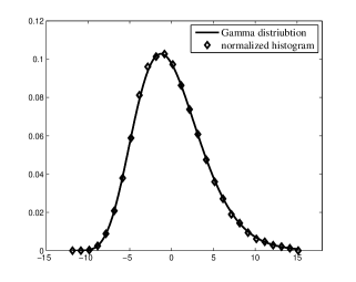
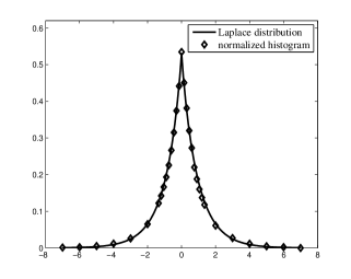
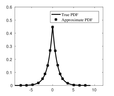
Before we discuss the approximation of the random noise, we first start with a full MD simulation, from which we can obtain the time series of $a(t)$ and $F(t)$. Our numerical test simulates an equilibrium system containing $500$ atoms which are evenly divided into $n=50$ blocks. The histograms of one entry of $a(t)$ and $F(t)$ at equilibrium are shown in Figure 2, which can be assumed to be the exact stationary distributions. Interestingly, both quantities exhibit non-Gaussian statistics. The PDF of $a(t)$ fits perfectly to a shifted Gamma distribution, and the PDF of the random noise follows a Laplace distribution. See Figure 2.

Figure 2: The left figure shows the histogram of $a_{1}(t)$ obtained from direct simulations. The data fits well to a shifted Gamma distribution $\Gamma_{\alpha,\beta}(x)\sim(x+\mu)^{\alpha-1}\exp(-\beta(x+\mu)),\;x\geq-\mu,$ with $\alpha=10.0596,\;\beta=0.7825$ and $\mu=\alpha/\beta$. The right figure shows the histogram of $F_{1}(t)$ and it fits a Laplace distribution $\text{Lap}_{b}(x)\sim\exp(-b|x|)$ with $b=1.0801$.

In the following section, we will focus on the approximation of the noise term so that the solution of the reduced models gives consistent statistics of the CG energy variables.

III.3 Approximation of the noise

In the previous section, we have discussed how the memory term can be approximated using the rational approximation in terms of the Laplace transforms. In particular, it gives rise to deterministic (or drift) terms in the resulting approximate models. Here, we discuss the approximation of the noise. We will consider both additive and multiplicative noises.

III.3.1 Approximations by additive noise

A natural (and most widely used) approximation is by a Gaussian white noise. For instance, for the first order approximation, we are led to a linear SDE,

$$\dot{{a}}(t)=-\Gamma{a}(t)+\sigma\zeta(t),$$ (3.46)

where $\zeta(t)$ is the standard Gaussian-white noise,

$$\left<\zeta(t_{1}),\zeta(t_{2})^{\intercal}\right>=\delta(t_{1}-t_{2}).$$ (3.47)

In order for the solution $a$ to have the correct covariance $M$, the parameter $\sigma$ has to satisfy the Lyapunov equation, risken1989fpe

$$\Sigma\overset{\Delta}{=}\sigma\sigma^{\intercal}=\Gamma M+M\Gamma^{\intercal}.$$ (3.48)

On the other hand, with the rational approximation (2.31) of the kernel function, we may introduce noise via the second equation. Namely,

$$\left\{\begin{aligned} \dot{{a}}(t)=&-z(t),\\ \dot{z}(t)=&B_{1}z(t)+A_{1}{a}(t)+\sigma\zeta(t).\end{aligned}\right.$$ (3.49)

It is clear that the second equation can be solved explicitly and substituted into the first equation, which would yield a similar equation to the GLE (2.6). By choosing the initial condition $z(0)$ and $\Sigma$ appropriately, the approximations to the memory kernel and the random noise can be made consistent, in terms of the second FDT (2.9).

Theorem 5.

Assuming the covariance of $z(0)$ is $A_{1}$, and

$$B_{1}A_{1}+A_{1}B_{1}^{\intercal}+\Sigma=0,$$ (3.50)

then, the extended system is equivalent to approximating the kernel function by $\theta_{1}(t)=e^{tB_{1}}A_{1}$, and the approximate noise, denoted by $F_{1}(t)$, to $F(t)$ satisfies the second FDT exactly. Namely,

$$\theta_{1}(t-t^{\prime})=\left<F_{1}(t),F_{1}(t^{\prime})\right>M^{-1},\quad\forall\;t,t^{\prime}\geq 0.$$

The proof of this theorem can be found in ma2016derivation .

The approximation by additive noises inevitably leads to a Gaussian distribution for $a(t)$ risken1989fpe . To check the validity of this assumption, we ran a direct simulation based on both the zeroth order model (3.46) and the first order model (3.49). The solutions are then compared to the true statistics, and the results are displayed in Figure 3.

Figure 3: The left figure shows the true PDF of $a_{1}$ and approximate PDF from approximations with Gaussian additive noise. The right panel shows the time correlation of approximate models.

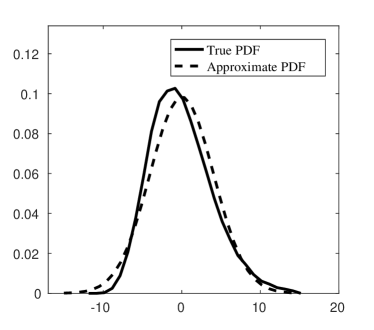
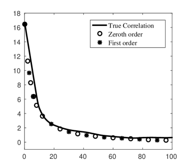
From Figure 3, we observe that although the time correlation of the CG energy is well captured, the PDF deviates from the true distribution.

III.3.2 Approximations using multiplicative noise

As alluded to in the previous section, the approximate model driven by Gaussian additive white noise may not capture the correct PDF. In this section, we consider multiplicative noise, with the objective of enforcing the correct equilibrium statistics for the solution of the SDEs.

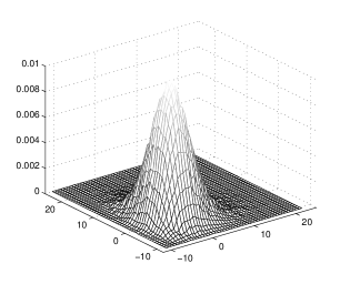
We start with a further observation that the energy of each block is almost independent to each other. Figure 4 shows the agreement between the joint histogram of the energy of two adjacent blocks and the true marginal PDFs. It is interesting that same observations have been made for biomolecules faure2017entropy . It is clearly difficult to prove the exact independence theoretically. Therefore, we keep this as our main assumption, and postulate the stationary PDF ($\rho(a)$) of the energy as a shifted multi-Gamma distribution with parameters $\alpha_{i}$ and $\beta_{i}$,

$$\rho(a)\propto\prod_{i=1}^{n}\left({a}_{i}-\frac{\alpha_{i}}{\beta_{i}}\right)^{\alpha_{i}-1}\!\!\!\!\!e^{-\beta_{i}\left({a}_{i}+\alpha_{i}/\beta_{i}\right)}.$$ (3.51)

Figure 4: The left figure shows the normalized joint histogram of $a_{1}$ and $a_{2}$ and the right panel shows the product of two normalized individual histogram of $a_{1}$ and $a_{2}$.

Now we reconsider the zeroth order approximation, the Markovian approximation by $R_{0,0}=\Theta(+\infty)=\Gamma.$ With a multiplicative noise, we are solving the following SDE,

$$\dot{a}(t)=-\Gamma a(t)+\sigma(a(t))\xi(t),$$ (3.52)

where $\xi(t)$ is the again standard Gaussian white noise. The SDE is interpreted in the Itô sense.

To derive a simple formula, we seek $\sigma$ in a diagonal form. We aim to construct $D\overset{\Delta}{=}2\sigma\sigma^{\intercal}$ to ensure the desired PDF given by (3.51). By simplifying the Fokker-Planck equation (FPE) that corresponds to (3.52), we obtain,

$$\frac{\partial D_{ii}\rho}{\partial a_{i}}=-\rho\left(\Gamma_{ii}a_{i}+\sum_{j=1,j\neq i}^{n}\Gamma_{ij}a_{j}\right).$$ (3.53)

By directly solving these differential equations, we obtained an explicit formula for the matrix $D$, as summarized in the following theorem, which can be proved by direct integration of (3.53).

Theorem 6.

If $\Gamma$ is a Z-matrix, i.e., the off-diagonal entries are non-positve, and $\Gamma$ is semi-positive definite, then there exists a diagonal matrix $D$ for which the multi-Gamma distribution (3.51) is a steady state solution of the Fokker-Planck equation. The diagonals of $D$ are given by,

$$D_{ii}=\frac{\Gamma_{ii}}{\beta_{i}}\left(a_{i}+\frac{\alpha_{i}}{\beta_{i}}\right)-\sum_{j=1,j\neq i}^{m}\Gamma_{ij}\frac{a_{j}\int_{-\frac{\alpha_{i}}{\beta_{i}}}^{a_{i}}\rho_{i}(x)dx+\alpha_{j}/\beta_{j}}{\rho_{i}(a_{i})}\geq 0,$$ (3.54)

where $\rho_{i}$ is the marginal PDF of $a_{i}$ and $\rho_{i}$ is propontional to $\left({a}_{i}+\frac{\alpha_{i}}{\beta_{i}}\right)^{\alpha_{i}-1}\!\!\!\!\!e^{-\beta_{i}\left({a}_{i}+\alpha_{i}/\beta_{i}\right)}$.

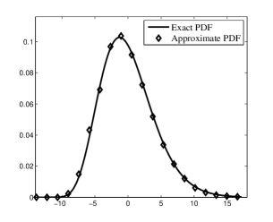
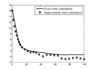
As a verification, we solved the SDEs (3.52) with coefficients determined by the above formula. Figure 5 shows the PDF of the first component along with its time correlation. Due to the uniform partition of the system, we expect the statistics to be the same for all the components of $a$. So we will only show the properties of the first component $a_{1}.$ It is clear that they are both consistent with the truth. It is worthwhile to point out that the SDE (3.52) contains a diffusion coefficient $\sigma$ which is unbounded. This can be viewed as a mechanism for the energy to stay above a lower bound. However, this introduces a stiff problem for the numerical approximation. To resolve this numerical issue, we applied the implicit Taylor method Tian2001implicit .

Figure 5: The left figure shows the approximate PDF of $a_{1}$ from the multiplicative model (3.52), along with the exact PDF. The right panel indicates the time correlation function.

Finally let’s turn to the model obtained by the first order approximation of the memory term. With Gaussian multiplicative noise, the first order model can be written formally as follows,

$$\left\{\begin{aligned} \dot{{a}}(t)=&-z(t),\\ \dot{z}(t)=&A{a}(t)+Bz(t)+\sigma(a(t),z(t))\xi(t),\end{aligned}\right.$$ (3.55)

where $A=A_{1}$ and $B=B_{1}$ are given in (2.32). This is a Langevin equation. But notice that in the multiplicative noise term, we allowed the diffusion coefficient to depend on both $a$ and $z.$

Again from the results of direct simulations, we observed that the components of $a$ and $z$ are independent. So we assume all these components are independent and its joint distribution function is written as,

$$\rho(a,z)\propto\prod_{i=1}^{n}\left({a}_{i}-\frac{\alpha_{i}}{\beta_{i}}\right)^{\alpha_{i}-1}\!\!\!\!\!e^{-\beta_{i}\left({a}_{i}+\alpha_{i}/\beta_{i}\right)}e^{-\gamma_{i}|z_{i}|}.$$ (3.56)

Similarly, we assume $\sigma$ to be diagonal and work with the steady state solution of the FPE, which can be written as,

$$\frac{\partial D_{ii}\rho}{\partial z_{i}}=\left(\sum_{j=1}^{n}A_{ij}a_{j}+\sum_{j=1,j\neq i}^{n}B_{ij}z_{j}-\frac{1}{\gamma_{i}^{2}}\frac{\partial W(a)}{\partial a_{i}}\right)\rho+B_{ii}z_{i}\rho-\frac{1}{\gamma_{i}}\frac{\partial W(a)}{\partial a_{i}}|z_{i}|\rho.$$ (3.57)

By integrating this equation, we have,

Theorem 7.

In (3.55), suppose $B$ has non-positive diagonal entries. We have for $i=1,2,\cdots,n$,

$$D_{ii}= -\frac{sgn(z_{i})}{\gamma_{i}}\left(1-e^{\gamma_{i}|z_{i}|}\right)\left(\sum_{j=1}^{n}A_{ij}a_{j}+\sum_{j=1,j\neq i}^{n}B_{ij}z_{j}-\frac{2}{\gamma_{i}^{2}}\frac{\partial W(a)}{\partial a_{i}}\right)+f_{1}e^{\gamma_{i}|z_{i}|}$$ (3.58)

$$+\frac{1}{\gamma_{i}^{2}}\frac{\partial W(a)}{\partial a_{i}}z_{i}+f_{2}e^{\gamma_{i}|z_{i}|}+B_{ii}\left(-\frac{1}{\gamma_{i}}|z_{i}|-\frac{1}{\gamma_{i}^{2}}+\frac{1}{\gamma_{i}^{2}}e^{\gamma_{i}|z_{i}|}\right)+f_{3}e^{\gamma_{i}|z_{i}|},$$

where

$$f_{1} =\frac{1}{\gamma_{i}}\left(\sum_{j=1}^{n}|A_{ij}||a_{j}|+\sum_{j=1,j\neq i}^{n}|B_{ij}||z_{j}|+\frac{2}{\gamma_{i}^{2}}\left(\beta_{i}+\frac{\alpha_{i}-1}{a_{i}+\mu_{i}}\right)\right),$$ (3.59)

$$f_{2} =\frac{1}{\gamma_{i}^{3}e}\left(\beta_{i}+\frac{\alpha_{i}-1}{a_{i}+\mu_{i}}\right),$$

$$f_{3} =-B_{ii}\frac{1}{\gamma_{i}^{2}},$$

Further, $D_{ii}$ are positive and $\rho$ given in (3.56) is a steady state solution of the FPE, if $\sigma$ is a diagonal matrix and $2\sigma_{ii}^{2}=D_{ii}$.

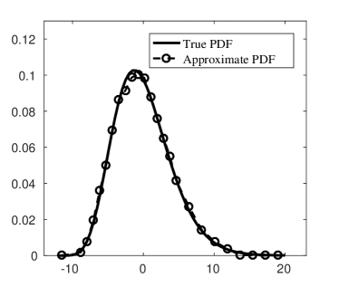
From Figure 6, we see that the first order model (3.55) is able to capture the statistics of both energy $a$ and $z$. Similar to the zeroth order model, the SDEs are stiff, and the implicit Taylor method Tian2001implicit with stepsize $\Delta t=5\times 10^{-4}$ is used to generate a long time series to obtain the statistics.

Figure 6: The left figure shows the comparison of the true PDF of $a_{1}$ and its approximation obtained from solving the first order SDE model (3.55) using the implicit Taylor method. The right panel shows the PDFs of $z_{1}$.

IV Summary and discussions

This work is concerned with a coarse-grained energy model directly obtained from the full molecular dynamics model. The goal is to find a more efficient model so that the heat conduction process can be simulated with a model that is a lot cheaper than non-equilibrium molecular dynamics simulations. Our focus has been placed on the equilibrium statistics of such models, which conceptually, is often a good starting point to develop a stochastic model. Unlike many of the coarse-grained molecular models, in which the coarse-grained velocity is expected to have Gaussian statistics, we found that the coarse-grained energy follows non-Gaussian statistics. We proposed to introduce multiplicative noise, within the Markovian embedding framework for the memory term, to ensure that the solution of the coarse-grained models has the correct equilibrium statistics.

Although we only considered a one-dimensional model as the example, the framework is applicable to more general systems. In particular, none of the theorems assumed the space dimensionality. The applications to nano-mechanical systems is currently underway.

This work suggests a new paradigms for modeling nano-scale transport phenomena in general: Rather than relying on traditional deterministic models, e.g., the Fourier’s Law and the Fick’s Law, one may derive from first-principle a stochastic and nonlocal constitutive relation for the mass or heat current. The extension of the current effort to general diffusion processes will be in the scope of our future work.

References

- [1] M. P. Allen and D. J. Tildesley. Computer Simulation of Liquids. Oxford University Press, 1989.
- [2] M. Baaden and S. J. Marrink. Coarse-grain modelling of protein-protein interactions. Current Opinion in Structural Biology, In press., Oct. 2013.
- [3] A. A. Balandin. Thermal properties of graphene and nanostructured carbon materials. Nature Materials, 10:569, 2011.
- [4] C. Bernardin and S. Olla. Fourier’s law for a microscopic model of heat conduction. Journal of Statistical Physics, 121(3-4):271–289, 2005.
- [5] P. L. Bhatnagar, E. P. Gross, and M. Krook. A model for collision processes in gases. i. small amplitude processes in charged and neutral one-component systems. Physical review, 94(3):511, 1954.
- [6] F. Bonetto, J. L. Lebowitz, and L. Rey-Bellet. Fourier’s law: A challenge for theorists. arXiv preprint math-ph/0002052, 2000.
- [7] J. Callaway. Model for lattice thermal conductivity at low temperatures. Phys. Rev., 113:1046–1051, 1959.
- [8] M. Ceriotti, G. Bussi, and M. Parrinello. Colored-noise thermostats à la carte. Journal of Chemical Theory and Computation, 6(4):1170–1180, 2010.
- [9] C. W. Chang, D. Okawa, H. Garcia, A. Majumdar, and A. Zettl. Breakdown of Fourier’s Law in nanotube thermal conductors. Phys. Rev. Lett., 101:075903, 2008.
- [10] J. Che, T. Caǧom, W. Deng, and W. A. G. III. Thermal conductivity of diamond and related materials from molecular dynamics simulations. J. Chem. Phys., 22:6888, 2000.
- [11] G. Chen. Ballistic-diffusive heat-conduction equations. Phys. Rev. Lett., 86:2297 2300, 2001.
- [12] J. Chen, G. Zhang, and B. Li. Molecular dynamics simulations of heat conduction in nanostructures: Effect of heat bath. J. Phys. Soc. Jpn., 79:074604, 2010.
- [13] K.-Q. Chen, W.-X. Li, W. Duan, Z. Shuai, and B.-L. Gu. Effect of defects on the thermal conductivity in a nanowire. Physical Review B, 72(4):045422, 2005.
- [14] Y. Chen, D. Li, J. Yang, Y. Wu, J. R. Lukes, and A. Majumdar. Molecular dynamics study of the lattice thermal conductivity of kr/ar superlattice nanowires. Physica B: Condensed Matter, 349(1):270–280, 2004.
- [15] A. J. Chorin and O. H. Hald. Stochastic tools in mathematics and science, volume 3. Springer, 2009.
- [16] A. J. Chorin, O. H. Hald, and R. Kupferman. Optimal prediction with memory. Phys. D, 166:239–257, 2002.
- [17] A. J. Chorin, A. Kast, and R. Kupferman. Optimal prediction of underresolved dynamics. Proc. Nat. Acad. Sci. USA, 96:4094 – 4098, 1998.
- [18] A. J. Chorin and P. Stinis. Problem reduction, renormalization, and memory. Comm. Appl. Math. Comp. Sc., 1:1–27, 2005.
- [19] B. Cockburn, S. Hou, and C. Shu. The Runge-Kutta local projection discontinuous Galerkin finite element method for conservation laws. IV: the multidimensional case. Math. Comp., 54(190):545–581, 1990.
- [20] C. Dames and G. Chen. Theoretical phonon thermal conductivity of si/ge superlattice nanowires. Journal of Applied Physics, 95(2):682–693, 2004.
- [21] D. Donadio and G. Galli. Atomistic simulations of heat transport in silicon nanowires. Phys. Rev. L, 102:195901, 2009.
- [22] D. Donadio and G. Galli. Atomistic simulations of heat transport in silicon nanowires. Physical review letters, 102(19):195901, 2009.
- [23] P. Espanol and P. Warren. Statistical mechanics of dissipative particle dynamics. EPL (Europhysics Letters), 30(4):191, 1995.
- [24] D. J. Evans and G. Morriss. Nonlinear-response theory for steady planar Couette flow. Physical Review A, 30:1528–1530, 1984.
- [25] D. J. Evans and G. P. Morriss. Statistical Mechanics of Non-equilibrium Liquids. ACADEMIC PRESS, 2008.
- [26] W. J. Evans, L. Hu, and P. Keblinski. Thermal conductivity of graphene ribbons from equilibrium molecular dynamics: Effect of ribbon width, edge roughness, and hydrogen termination. Applied physics letters, 96(20):203112–203112, 2010.
- [27] G. Faure, R. Delgado-Buscalioni, and P. Español. The entropy of a complex molecule. The Journal of Chemical Physics, 146(22):224106, 2017.
- [28] D. Frenkel and B. Smit. Understanding Molecular Simulation: From Algorithms to Applications. Academic Press, 2nd edition, 2002.
- [29] M. Fujii, X. Zhang, H. Xie, H. Ago, K. Takahashi, T. Ikuta, H. Abe, and T. Shimizu. Measuring the thermal conductivity of a single carbon nanotube. Phys. Rev. Lett., 95:065502, 2005.
- [30] P. L. Garrido, P. I. Hurtado, and B. Nadrowski. Simple one-dimensional model of heat conduction which obeys Fourier’s law. Physical Review Letters, 86(24):5486, 2001.
- [31] S. Gill, Z. Jia, B. Leimkuhler, and A. Cocks. Rapid thermal equilibration in coarse-grained molecular dynamics. Physical Review B, 73(18):184304, 2006.
- [32] H. Gohlke and M. Thorpe. A natural coarse graining for simulating large biomolecular motion. Biophysical Journal, 91(6):2115–2120, Sept. 2006.
- [33] P. A. Golubkov and P. Ren. Generalized coarse-grained model based on point multipole and Gay-Berne potentials. The Journal of Chemical Physics, 125(6):064103, 2006.
- [34] A. Gramada and P. E. Bourne. Coarse-graining the electrostatic potential via distributed multipole expansions. Computer Physics Communications, 182(7):1455–1462, July 2011.
- [35] A. S. Henry and G. Chen. Spectral phonon transport properties of Silicon based on molecular dynamics simulations and lattice dynamics. J. Comput. Theor. Nanosci., 5:1–12, 2008.
- [36] C. Hijón, M. Serrano, and P. Español. Markovian approximation in a coarse-grained description of atomic systems. J. Chem. Phys., 125:204101, 2006.
- [37] J. Hone, M. Whitney, C. Piskoti, and A. Zettl. Thermal conductivity of single-walled carbon nanotubes. Physical Review B, 59(4):R2514, 1999.
- [38] J. Hu, X. Ruan, and Y. P. Chen. Thermal conductivity and thermal rectification in graphene nanoribbons: a molecular dynamics study. Nano Letters, 9(7):2730–2735, 2009.
- [39] S. Izvekov and G. A. Voth. Modeling real dynamics in the coarse-grained representation of condensed phase systems. J. Chem. Phys., 125:151101–151104, 2006.
- [40] K. Jolley and S. Gill. Modelling transient heat conduction in solids at multiple length and time scales: A coupled non-equilibrium molecular dynamics/continuum approach. Journal of Computational Physics, 228(19):7412–7425, 2009.
- [41] A. Joshi and A. Majumdar. Transient ballistic and diffusive phonon heat transport in thin films. J. Appl. Phys., 74:31, 1993.
- [42] M. A. Katsoulakis, A. J. Majda, and D. G. Vlachos. Coarse-grained stochastic processes for lattice systems. Proc. Natl. Acad. Sci. USA, 100:782–787, 2003.
- [43] D. Kauzlarić, P. Español, A. Greiner, and S. Succi. Markovian dissipative coarse grained molecular dynamics for a simple 2d graphene model. The Journal of chemical physics, 137(23):234103, 2012.
- [44] P. Kim, L. Shi, A. Majumdar, and P. McEuen. Thermal transport measurements of individual multiwalled nanotubes. Phys. Rev. Lett, 87:215502, 2001.
- [45] R. Kubo. The fluctuation-dissipation theorem. Reports on Progress in Physics, 29(1):255 – 284, 1966.
- [46] H. Lei, N. A. Baker, and X. Li. Data-driven parameterization of the generalized Langevin equation. Proceedings of the National Academy of Sciences, 113(50):14183–14188, 2016.
- [47] S. Lepri, R. Livi, and A. Politi. Heat conduction in chains of nonlinear oscillators. Physical review letters, 78(10):1896, 1997.
- [48] S. Lepri, R. Livi, and A. Politi. On the anomalous thermal conductivity of one-dimensional lattices. EPL (Europhysics Letters), 43(3):271, 1998.
- [49] S. Lepri, R. Livi, and A. Politi. Thermal conduction in classical low-dimensional lattices. Physics Reports, 377(1):1–80, 2003.
- [50] D. Li, Y. Wu, P. Kim, L. Shi, P. Yang, and A. Majumdar. Thermal conductivity of individual silicon nanowires. Applied Physics Letters, 83(14):2934–2936, 2003.
- [51] X. Li. A coarse-grained molecular dynamics model for crystalline solids. Int. J. Numer. Meth. Engng., 83:986–997, 2010.
- [52] X. Lu, W. Shen, and J. Chu. Size effect on the thermal conductivity of nanowires. Journal of applied physics, 91(3):1542–1552, 2002.
- [53] L. Ma, X. Li, and C. Liu. The derivation and approximation of coarse-grained dynamics from Langevin dynamics. The Journal of Chemical Physics, 145(20):204117, 2016.
- [54] A. Majumdar. Microscale heat conduction in dielectric thin films. ASME Journal of Heat Transfer, 115:7–16, 1993.
- [55] S. Maruyama. A molecular dynamics simulation of heat conduction in finite length swnts. Physica B: Condensed Matter, 323(1):193–195, 2002.
- [56] S. Maruyama. A molecular dynamics simulation of heat conduction of a finite length single-walled carbon nanotube. Microscale Thermophysical Engineering, 7(1):41–50, 2003.
- [57] A. J. H. McGaughey and M. Ka. Phonon transport in molecular dynamics simulations: Formulation and thermal conductivity prediction. Advances in Heat Transfer, 39:169, 2006.
- [58] A. J. H. McGaughey and M. Kaviany. Thermal conductivity decomposition and analysis using molecular dynamics simulations. part I. Lennard-Jones argon. International Journal of Heat and Mass Transfer, 47:1783–1798, 2003.
- [59] H. Mori. A continued-fraction representation of the time-correlation functions. Progress of Theoretical Physics, 34:399–416, Sept. 1965.
- [60] H. Mori. Transport, collective motion, and Brownian motion. Prog. Theor. Phys., 33:423 – 450, 1965.
- [61] G. P. Morriss and D. J. Evans. Application of transient correlation functions to shear flow far from equilibrium. Physical Review A, 35(2):792, 1987.
- [62] S. O. Nielsen, R. E. Bulo, P. B. Moore, and B. Ensing. Recent progress in adaptive multiscale molecular dynamics simulations of soft matter. Physical Chemistry Chemical Physics, 12(39):12401, 2010.
- [63] W. G. Noid. Perspective: Coarse-grained models for biomolecular systems. The Journal of Chemical Physics, 139(9):090901, 2013.
- [64] W. G. Noid, J.-W. Chu, G. S. Ayton, V. Krishna, S. Izvekov, G. A. Voth, A. Das, and H. C. Andersen. The multiscale coarse-graining method. i. a rigorous bridge between atomistic and coarse-grained models. The Journal of Chemical Physics, 128(24):244114, 2008.
- [65] S. Nosé. A molecular dynamics method for simulations in the canonical ensemble. Mol. Phys., 52(2):255–268, 1984.
- [66] M. A. Osman and D. Srivastava. Temperature dependence of the thermal conductivity of single-wall carbon nanotubes. Nanotechnology, 12(1):21, 2001.
- [67] R. E. Peierles. Quantum Theory of Solids. Academic Press, 1955.
- [68] E. Pop, D. Mann, Q. Wang, K. Goodson, and H. Dai. Thermal conductance of an individual single-wall carbon nanotube above room temperature. Nano Letters, 6:96–100, 2006.
- [69] P. Poulain, A. Saladin, B. Hartmann, and C. Pravost. Insights on protein-DNA recognition by coarse grain modelling. Journal of computational chemistry, 29(15):2582–2592, 2008.
- [70] M. Praprotnik, L. D. Site, and K. Kremer. Multiscale simulation of soft matter: From scale bridging to adaptive resolution. Annual Review of Physical Chemistry, 59(1):545–571, May 2008.
- [71] S. Riniker, J. R. Allison, and W. F. van Gunsteren. On developing coarse-grained models for biomolecular simulation: a review. Physical Chemistry Chemical Physics, 14(36):12423, 2012.
- [72] M. Ripoll, P. Español, and M. H. Ernst. Dissipative particle dynamics with energy conservation: Heat conduction. International Journal of Modern Physics C, 9(08):1329–1338, 1998.
- [73] H. Risken and H. Haken. The Fokker-Planck Equation: Methods of Solution and Applications Second Edition. Springer, 1989.
- [74] R. E. Rudd and J. Q. Broughton. Coarse-grained molecular dynamics and the atomic limit of finite element. Phys. Rev. B, 58(10):5893 – 5896, 1998.
- [75] R. E. Rudd and J. Q. Broughton. Coarse-grained molecular dynamics: Nonlinear finite elements and finite temperature. Phys. Rev. B, 72:144104, 2005.
- [76] J. F. Rudzinski and W. G. Noid. The role of many-body correlations in determining potentials for coarse-grained models of equilibrium structure. The Journal of Physical Chemistry B, 116(29):8621–8635, July 2012.
- [77] A. V. Savin, Y. S. Kivshar, and B. Hu. Suppression of thermal conductivity in graphene nanoribbons with rough edges. arXiv preprint arXiv:1006.4879, 2010.
- [78] P. K. Schelling, S. R. Phillpot, and P. Keblinski. Comparison of atomic-level simulation methods for computing thermal conductivity. Phys. Rev. B, 65:144306, 2002.
- [79] Q. Shi, P. Liu, and G. A. Voth. Coarse-graining in interaction space: An analytical approximation for the effective short-ranged electrostatics. The Journal of Physical Chemistry B, 112(50):16230–16237, Dec. 2008.
- [80] S. Silling and R. B. Lehoucq. Statistical coarse-graining of molecular dynamics into peridynamics. Technical report, Sandia National Laboratories SAND2007-6410, 2007.
- [81] G. Simonelli, R. Pasianot, and E. J. Savino. Phonon dispersion curves for transition metals within the embedded-atom and embedded-defect methods. Phys. Rev. B, 55:5570 5573, 1997.
- [82] M. Stepanova. Dynamics of essential collective motions in proteins: Theory. Physical Review E, 76:051918, 2007.
- [83] P. Sverdrup, Y. Ju, and K. Goodson. Sub-continuum simulations of heat conduction in silicon-on-insulator transistors. ASME J. Heat Transfer, 123:130 137, 2001.
- [84] T. Tian and K. Burrage. Implicit Taylor methods for stiff stochastic differential equations. Applied Numerical Mathematics, 38(1-2):167–185, 2001.
- [85] M. Toda, R. Kubo, and N. Hashitsume. Statistical Physics II. Non-equilibrium Statistical Mechanics. Springer, 1983.
- [86] D. Tzou. Nonlocal behavior in phonon transport. International Journal of Heat and Mass Transfer, 15:475 481, 2011.
- [87] D. Y. Tzou. Experimental support for the lagging behavior in heat propagation. Journal of Thermophysics and Heat Transfer, 9(4):686–693, 1995.
- [88] A. N. Volkova and L. V. Zhigileib. Heat conduction in carbon nanotube materials: Strong effect of intrinsic thermal conductivity of carbon nanotubes. Appl. Phys. Lett., 101:043113, 2012.
- [89] S. G. Volz and G. Chen. Molecular dynamics simulation of thermal conductivity of silicon nanowires. Applied Physics Letters, 75(14):2056–2058, 1999.
- [90] S. G. Volz and G. Chen. Molecular-dynamics simulation of thermal conductivity of silicon crystals. Phys. Rev. B, 61:2651, 2000.
- [91] J. Wang. Quantum thermal transport from classical molecular dynamics. Phys. Rev. Le, 99:160601, 2007.
- [92] L. Wang, B. Hu, and B. Li. Logarithmic divergent thermal conductivity in two-dimensional nonlinear lattices. Phys. Rev. E, 86:040101, 2012.
- [93] S.-C. Wang, X.-G. Liang, X.-H. Xu, and T. Ohara. Thermal conductivity of silicon nanowire by nonequilibrium molecular dynamics simulations. Journal of Applied Physics, 105(1):014316–014316, 2009.
- [94] P. L. Williams, Y. Mishin, and J. C. Hamilton. An embedded-atom potential for the CuAg system. Modelling Simul. Mater. Sci. Eng., 14:817 833, 2006.
- [95] M. Xu and X. Li. The modeling of nanoscale heat conduction by Boltzmann transport equation. International Journal of Heat and Mass Transfer, 55:1905 1910, 2012.
- [96] C. Yu, L. Shi, Z. Yao, D. Li, and A. Majumdar. Thermal conductance and thermopower of an individual single-wall carbon nanotube. Nano Letters, 5(9):1842–1846, 2005.
- [97] Z. Zhang, L. Lu, W. G. Noid, V. Krishna, J. Pfaendtner, and G. A. Voth. A systematic methodology for defining coarse-grained sites in large biomolecules. Biophysical Journal, 95(11):5073–5083, Dec. 2008.
- [98] J. M. Ziman. Electrons and Phonons. Oxford University Press, 2001.
- [99] R. Zwanzig. Nonlinear generalized Langevin equations. J. Stat. Phys., 9:215 – 220, 1973.
- [100] R. Zwanzig. Problems in nonlinear transport theory. In Systems far from equilibrium, Ed. L. Garrido. Interscience, New York, 1980.
- [101] R. Zwanzig. Nonequilibrium Statistical Mechanics. Oxford University Press, 2001.