Nonparametric Shape-restricted Regression

Abstract

We consider the problem of nonparametric regression under shape constraints. The main examples include isotonic regression (with respect to any partial order), unimodal/convex regression, additive shape-restricted regression, and constrained single index model. We review some of the theoretical properties of the least squares estimator (LSE) in these problems, emphasizing on the adaptive nature of the LSE. In particular, we study the behavior of the risk of the LSE, and its pointwise limiting distribution theory, with special emphasis to isotonic regression. We survey various methods for constructing pointwise confidence intervals around these shape-restricted functions. We also briefly discuss the computation of the LSE and indicate some open research problems and future directions.

and

t1Supported by NSF CAREER Grant DMS-16-54589. t2Supported by NSF Grants DMS-17-12822 and AST-16-14743.

1 Introduction

In nonparametric shape-restricted regression the observations $\{(x_{i},y_{i}):i=1,\ldots,n\}$ satisfy

$$y_{i}=f(x_{i})+\varepsilon_{i},\qquad\mbox{for }i=1,\ldots,n,$$ (1)

where $x_{1},\ldots,x_{n}$ are design points in some space (e.g., $\mathbb{R}^{d}$, $d\geq 1$), $\varepsilon_{1},\ldots,\varepsilon_{n}$ are unobserved mean-zero errors (with finite variances), and the real-valued regression function $f$ is unknown but obeys certain known qualitative restrictions like monotonicity, convexity, etc. Let $\mathcal{F}$ denote the class of all such regression functions. Letting $\theta^{*}:=(f(x_{1}),\ldots,f(x_{n}))$, $Y:=(y_{1},\ldots,y_{n})$ and $\varepsilon:=(\varepsilon_{1},\ldots,\varepsilon_{n})$, model (1) may be rewritten as

$$Y=\theta^{*}+\varepsilon,$$ (2)

and the problem is to estimate $\theta^{*}$ and/or $f$ from $Y$, subject to the constraints imposed by the properties of $\mathcal{F}$. The constraints on the function class $\mathcal{F}$ translate to constraints on $\theta^{*}$ of the form $\theta^{*}\in\mathcal{C}$, where

$$\mathcal{C}:=\big{\{}(f(x_{1}),\dots,f(x_{n}))\in\mathbb{R}^{n}:f\in\mathcal{F}\big{\}}$$ (3)

is a subset of $\mathbb{R}^{n}$ (in fact, in most cases, $\mathcal{C}$ will be a closed convex cone). In the following we give some examples of shape-restricted regression.

Example 1.1 (Isotonic regression).

Probably the most studied shape-restricted regression problem is that of estimating a monotone (nondecreasing) regression function $f$ when $x_{1}<\ldots<x_{n}$ are the univariate design points. In this case, $\mathcal{F}$ is the class of all nondecreasing functions on the interval $[x_{1},x_{n}]$, and the constraint set $\mathcal{C}$ reduces to

$$\mathcal{I}:=\{(\theta_{1},\ldots,\theta_{n})\in\mathbb{R}^{n}:\theta_{1}\leq\ldots\leq\theta_{n}\},$$ (4)

which is a closed convex cone in $\mathbb{R}^{n}$ ($\mathcal{I}$ is defined through $n-1$ linear constraints). The above problem is typically known as isotonic regression and has a long history in statistics; see e.g., [23, 5, 138].

Example 1.2 (Order preserving regression on a partially ordered set).

Isotonic regression can be easily extended to the setup where the covariates take values in a space $\mathcal{X}$ with a partial order $\precsim$; see e.g., [118, Chapter 1]. A function $f:\mathcal{X}\to\mathbb{R}$ is said to be isotonic (or order preserving) with respect to the partial order $\precsim$ if for every pair $u,v\in\mathcal{X}$,

$$u\precsim v\;\;\Rightarrow\;\;f(u)\leq f(v).$$

For example, suppose that the predictors take values in $\mathbb{R}^{2}$ and the partial order $\precsim$ is defined as $(u_{1},u_{2})\precsim(v_{1},v_{2})$ if and only if $u_{1}\leq v_{1}$ and $u_{2}\leq v_{2}$. This partial order leads to a natural extension of isotonic regression to two dimensions; see e.g., [71, 117, 29]. One can also consider other partial orders; see e.g., [131, 132] and the references therein for isotonic regression with different partial orders. We will introduce and study yet another partial order in Section 6.

Given data from model (1), the goal is to estimate the unknown regression function $f:\mathcal{X}\to\mathbb{R}$ under the assumption that $f$ is order preserving (with respect to the partial order $\precsim$). The restrictions imposed by the partial order $\precsim$ constrain $\theta^{*}$ to lie in a closed convex cone $\mathcal{C}$ which may be expressed as

$$\{(\theta_{1},\ldots,\theta_{n})\in\mathbb{R}^{n}:\theta_{i}\leq\theta_{j}\mbox{ for every }i,j\mbox{ such that }x_{i}\precsim x_{j}\}.$$

Example 1.3 (Convex regression).

Suppose that the underlying regression function $f:\mathbb{R}^{d}\to\mathbb{R}$ ($d\geq 1$) is known to be convex, i.e., for every $u,v\in\mathbb{R}^{d}$,

$$f(\alpha u+(1-\alpha)v)\leq\alpha f(u)+(1-\alpha)f(v),\quad\mbox{ for every }\alpha\in(0,1).$$ (5)

Convexity appears naturally in many applications; see e.g., [73, 86, 38] and the references therein. The convexity of $f$ constrains $\theta^{*}$ to lie in a (polyhedral) convex set $\mathcal{C}\subset\mathbb{R}^{n}$ which, when $d=1$ and the $x_{i}$’s are ordered, reduces to

$$\mathcal{K}:=\left\{(\theta_{1},\ldots,\theta_{n})\in\mathbb{R}^{n}:\frac{\theta_{2}-\theta_{1}}{x_{2}-x_{1}}\leq\ldots\leq\frac{\theta_{n}-\theta_{n-1}}{x_{n}-x_{n-1}}\right\},$$ (6)

whereas for $d\geq 2$ the characterization of $\mathcal{C}$ is more complex; see e.g., [121].

Observe that when $d=1$, convexity is characterized by nondecreasing derivatives (subgradients). This observation can be used to generalize convexity to $k$-monotonicity ($k\geq 1$): a real-valued function $f$ is said to be $k$-monotone if its $(k-1)$’th derivative is monotone; see e.g., [94, 28]. For equi-spaced design points in $\mathbb{R}$, this restriction constrains $\theta^{*}$ to lie in the set

$$\{\theta\in\mathbb{R}^{n}:\nabla^{k}\theta\geq 0\}$$

where $\nabla:\mathbb{R}^{n}\rightarrow\mathbb{R}^{n}$ is given by $\nabla(\theta):=(\theta_{2}-\theta_{1},\theta_{3}-\theta_{2},\dots,\theta_{n}-\theta_{n-1},0)$ and $\nabla^{k}$ represents the $k$-times composition of $\nabla$. Note that the case $k=1$ and $k=2$ correspond to isotonic and convex regression, respectively.

Example 1.4 (Unimodal regression).

In many applications $f$, the underlying regression function, is known to be unimodal; see e.g., [49, 27] and the references therein. Let $\mathcal{I}_{m}$, $1\leq m\leq n$, denote the convex set of all unimodal vectors (first decreasing and then increasing) with mode at position $m$, i.e.,

$$\mathcal{I}_{m}:=\{(\theta_{1},\ldots,\theta_{n})\in\mathbb{R}^{n}:\theta_{1}\geq\ldots\geq\theta_{m}\leq\theta_{m+1}\leq\ldots\leq\theta_{n}\}.$$

Then, the unimodality of $f$ constrains $\theta^{*}$ to belong to $\mathcal{U}:=\cup_{m=1}^{n}\mathcal{I}_{m}$. Observe that now $\mathcal{U}$ is not a convex set, but a union of $n$ convex cones.

Example 1.5 (Shape-restricted additive model).

In an additive regression model one assumes that $f:\mathbb{R}^{d}\to\mathbb{R}$ ($d\geq 1$) depends on each of the predictor variables in an additive fashion, i.e., for $(u_{1},\ldots,u_{d})\in\mathbb{R}^{d}$,

$$f(u_{1},\ldots,u_{d})=\sum_{i=1}^{d}f_{i}(u_{i}),$$

where $f_{i}$’s are one-dimensional functions and $f_{i}$ captures the influence of the $i$’th variable. Observe that the additive model generalizes (multiple) linear regression. If we assume that each of the $f_{i}$’s are shape-constrained, then one obtains a shape-restricted additive model; see e.g., [6, 97, 105, 35] for a study of some possible applications, identifiability and estimation in such a model.

Example 1.6 (Shape-restricted single index model).

In a single index regression model one assumes that the regression function $f:\mathbb{R}^{d}\to\mathbb{R}$ takes the form

$$f(x)=m(x^{\top}\beta^{*}),\quad\mbox{ for all }\,x\in\mathbb{R}^{d},$$

where $m:\mathbb{R}\to\mathbb{R}$ and $\beta^{*}\in\mathbb{R}^{d}$ are unknown. Single index models are popular in many application areas, including econometrics and biostatistics (see e.g., [114, 90]), as they circumvent the curse of dimensionality encountered in estimating the fully nonparametric regression function by assuming that the link function depends on $x$ only through a one-dimensional projection, i.e., $x^{\top}\beta^{*}$. Moreover, the coefficient vector $\beta^{*}$ provides interpretability. Observe that single index models extend generalized linear models (where the link function $m$ is assumed known). Moreover, as most known link functions are nondecreasing, the monotone single index model (where $m$ is assumed unknown but nondecreasing) arises naturally in applications; see e.g., [108, 57, 9].

Observe that all the aforementioned problems fall under the general area of nonparametric regression. However, it turns out that in each of the above problems one can use classical techniques like least squares and/or maximum likelihood (without additional explicit regularization/penalization) to readily obtain tuning parameter-free estimators that have attractive theoretical and computational properties. This makes shape-restricted regression different from usual nonparametric regression, where likelihood based methods are generally infeasible. In this paper we try to showcase some of these attractive features of shape-restricted regression and give an overview of the major theoretical advances in this area.

Let us now introduce the estimator of $\theta^{*}$ (and $f$) that we will study in this paper. The least squares estimator (LSE) $\hat{\theta}$ of $\theta^{*}$ in shape-restricted regression is defined as the projection of $Y$ onto the set $\mathcal{C}$ (see (3)), i.e.,

$$\hat{\theta}:=\arg\min_{\theta\in\mathcal{C}}\|Y-\theta\|^{2},$$ (7)

where $\|\cdot\|$ denotes the usual Euclidean norm in $\mathbb{R}^{n}$. If $\mathcal{C}$ is a closed convex set then $\hat{\theta}\in\mathcal{C}$ is unique and is characterized by the following condition:

$$\langle Y-\hat{\theta},\theta-\hat{\theta}\rangle\leq 0,\quad\mbox{for all }\theta\in\mathcal{C},$$ (8)

where $\langle\cdot,\cdot\rangle$ denotes the usual inner product in $\mathbb{R}^{n}$; see [20, Proposition 2.2.1]. It is easy to see now that the LSE $\hat{\theta}$ is tuning parameter-free, unlike most nonparametric estimators. However it is not generally easy to find a closed-form expression for $\hat{\theta}$. As for estimating $f$, any $\hat{f}_{n}\in\mathcal{F}$ that agrees with $\hat{\theta}$ at the data points $x_{i}$’s will be considered as a LSE of $f$.

In this paper we mainly review the main theoretical properties of the LSE $\hat{\theta}$ with special emphasis on its adaptive nature. The risk behavior of $\hat{\theta}$ (in estimating $\theta^{*}$) is studied in Sections 2 and 3 — Section 2 mainly deals with the isotonic LSE in detail whereas Section 3 summarizes the main results for other shape-restricted problems. In Section 4 we study the pointwise asymptotic behavior of the LSE $\hat{f}_{n}$, in the case of isotonic and convex regression, focusing on methods for constructing (pointwise) confidence intervals around $f$. In the process of this review we highlight the main ideas and techniques used in the proofs of the theoretical results; in fact, we give (nearly) complete proofs in some cases.

The computation of the LSE $\hat{\theta}$, in the various problems outlined above, is discussed in Section 5. In Section 6 we mention a few open research problems and possible future directions. Although the paper mostly summarizes known results, we also present some new results — Theorems 2.1, 2.2, 2.3, and 6.1, and Lemma 3.1 are new. Appendix A contains some of the detailed proofs of results in this paper.

There are indeed many other important applications and examples of shape-restricted regression beyond those highlighted so far. We briefly mention some of these below. Shape constrained functions also arise naturally in interval censoring problems (e.g., in the current status model; see [65, 76]), in survival analysis (e.g., in estimation of monotone/unimodal hazard rates [75]), and in regression models where the response, conditional on the covariate, comes from a regular parametric family (e.g., monotone response models [13]). It also arises in the study of many inverse problems; e.g., deconvolution problems (see e.g., [65, 77]) and the classical Wicksell’s corpuscle problem (see e.g., [58, 124]). There are many applications that involve testing with shape constraints; see e.g., [44, 123, 140] and the references therein.

In this paper we will mostly focus on estimation of the underlying shape-restricted function using the method of least squares. Although this produces tuning parameter-free estimators, the obtained LSEs are not “smooth”. There is also a line of research that combines shape constraints with smoothness assumptions — see e.g., [107, 93, 64] (and the references therein) where kernel-based methods have been combined with shape-restrictions, and see [96, 104, 108, 84] where splines are used in conjunction with the shape constraints.

1.1 Some applications of shape-restricted regression

Shape-constrained regression has a long history in statistics: Hildreth [73] considered least squares estimation (i.e., maximum likelihood estimation under Gaussian errors) of production functions under the natural assumption of nonincreasing returns (which implies that the production function is concave and nondecreasing). Around the same time, Brunk [23] considered maximum likelihood estimation of a regression function under monotonicity constraints. Since then isotonic regression (under any partial order) has seen many applications in diverse settings: in biology [111], in dose-response models [74], in psychology [83], in genetics [91], etc.

Similarly, convexity or concavity constraints arise natural in many disciplines. Economic theory dictates that utility functions are increasing and concave [100] whereas production functions are often assumed to be concave [139]. In finance, theory restricts call option prices to be convex and decreasing functions of the strike price [2]; in stochastic control, value functions are often assumed to be convex (see [79] [12, Chapter 2] and [127]); see [92] for some applications of convex regression in optimization (in particular, in linear programming).

Unimodal regression also arises in many settings; see [49] and the references therein. Shape-restricted additive and single-index regression models offer flexible, yet interpretable, statistical procedures for handling multidimensional covariates, and have been extensively used in econometrics, epidemiology and other fields (see [35, 116, 84] and the references therein).

2 Risk bounds in Isotonic Regression

In this section we attempt to answer the following question: “How good is $\hat{\theta}$ as an estimator of $\theta^{*}$?”. To quantify the accuracy of $\hat{\theta}$ we first need to fix a loss function. Arguably the most natural loss function here is the squared error loss: $\lVert\hat{\theta}-\theta^{*}\rVert^{2}/n$. As the loss function is random, we follow the usual approach and study its expectation:

$$R(\hat{\theta},\theta^{*}):=\frac{1}{n}\mathbb{E}_{\theta^{*}}\big{[}\|\hat{\theta}-\theta^{*}\|^{2}\big{]}=\frac{1}{n}\mathbb{E}_{\theta^{*}}\sum_{i=1}^{n}\big{(}\hat{\theta}_{i}-\theta^{*}_{i}\big{)}^{2}$$ (9)

which we shall refer to as the risk of the LSE $\hat{\theta}$. We focus on the risk in this paper. It may be noted that upper bounds derived for the risk usually hold on the loss $\|\hat{\theta}-\theta^{*}\|^{2}/n$ as well, with high probability. When $\varepsilon\sim N_{n}(0,\sigma^{2}I_{n})$, this is essentially because $\|\hat{\theta}-\theta^{*}\|$ concentrates around its mean; see [136] and [19] for more details on high probability results.

One can also try to study the risk under more general $\ell_{p}$-loss functions. For $p\geq 1$, let

$$R^{(p)}(\hat{\theta},\theta^{*}):=\frac{1}{n}\mathbb{E}_{\theta^{*}}\big{[}\|\hat{\theta}-\theta^{*}\|_{p}^{p}\big{]}=\frac{1}{n}\mathbb{E}_{\theta^{*}}\sum_{i=1}^{n}\big{|}\hat{\theta}_{i}-\theta^{*}_{i}\big{|}^{p}$$ (10)

where $\lVert u\rVert_{p}:=\left(\sum_{j=1}^{n}|u_{j}|^{p}\right)^{1/p}$, for $u=(u_{1},\ldots,u_{n})\in\mathbb{R}^{n}$. We shall mostly focus on the risk for $p=2$ in this paper but we shall also discuss some results for $p\neq 2$.

In this section, we focus on the problem of isotonic regression (Example 1.1) and describe bounds on the risk of the isotonic LSE. As mentioned in the Introduction, isotonic regression is the most studied problem in shape-restricted regression where the risk behavior of the LSE is well-understood. We shall present the main results here. The results described in this section will serve as benchmarks to which risk bounds for other shape-restricted regression problems (see Section 3) can be compared.

Throughout this section, $\hat{\theta}$ will denote the isotonic LSE (which is the minimizer of $\|Y-\theta\|^{2}$ subject to the constraint that $\theta$ lies in the closed convex cone $\mathcal{I}$ described in (4)) and $\theta^{*}$ will usually denote an arbitrary vector in $\mathcal{I}$ (in some situations we deal with misspecified risks where $\theta^{*}$ is an arbitrary vector in $\mathbb{R}^{n}$ not necessarily in $\mathcal{I}$).

The risk, $R(\hat{\theta},\theta^{*})$, essentially has two different kinds of behavior. As long as $\theta^{*}\in\mathcal{I}$ and $V(\theta^{*}):=\theta_{n}^{*}-\theta^{*}_{1}$ (referred to as the variation of $\theta^{*}$) is bounded from above independently of $n$, the risk $R(\hat{\theta},\theta^{*})$ is bounded from above by a constant multiple of $n^{-2/3}$. We shall refer to this $n^{-2/3}$ bound as the worst case risk bound mainly because it is, in some sense, the maximum possible rate at which $R(\hat{\theta},\theta^{*})$ converges to zero. On the other hand, if $\theta^{*}\in\mathcal{I}$ is piecewise constant with not too many constant pieces, then the risk $R(\hat{\theta},\theta^{*})$ is bounded from above by the parametric rate $1/n$ up to a logarithmic multiplicative factor. This rate is obviously much faster compared to the worst case rate of $n^{-2/3}$ which means that the isotonic LSE is estimating piecewise constant nondecreasing sequences at a much faster rate. In other words, the isotonic LSE is adapting to piecewise constant nondecreasing sequences with not too many constant pieces. We shall therefore refer to this $\log n/n$ risk bound as the adaptive risk bound.

The worst case risk bounds for the isotonic LSE will be explored in Section 2.1 while the adaptive risk bounds are treated in Section 2.2. Proofs will be provided in the Appendix A. Before proceeding to risk bounds, let us first describe some basic properties of the isotonic LSE.

An important fact about the isotonic LSE is that $\hat{\theta}=(\hat{\theta}_{1},\dots,\hat{\theta}_{n})$ can be explicitly represented as (see [118, Chapter 1]):

$$\hat{\theta}_{j}=\min_{v\geq j}\max_{u\leq j}\frac{\sum_{l=u}^{v}y_{l}}{v-u+1},\quad\mbox{for }j=1,\ldots,n.$$ (11)

This is often referred to as the min-max formula for isotonic regression. The isotonic LSE is, in some sense, unique among shape-restricted regression LSEs because it has the above explicit characterization. It is this characterization that allows for a precise study of the properties of $\hat{\theta}$.

The above characterization of the isotonic LSE shows that $\hat{\theta}$ is piecewise constant, and in each “block” (i.e., region of constancy) it is the average of the response values (within the block); see [118, Chapter 1]. However, the blocks, their lengths and their positions, are chosen adaptively by the algorithm, the least squares procedure. If $\theta^{*}_{i}=f(x_{i})$ for some design points $0\leq x_{1}<\dots<x_{n}\leq 1$, then we can define the isotonic LSE of $f$ as the piecewise constant function $\hat{f}_{n}:[0,1]\to\mathbb{R}$ which has jumps only at the design points and such that $\hat{f}_{n}(x_{i})=\hat{\theta}_{i}$ for each $i=1,\ldots,n$. Figure 1 shows three different scatter plots, for three different regression functions $f$, with the fitted isotonic LSEs $\hat{f}_{n}$. Observe that for the leftmost plot the block-sizes (of the isotonic LSE) vary considerably with the change in slope of the underlying function $f$ — the isotonic LSE, $\hat{f}_{n}$, is nearly constant in the interval $[0.3,0.7]$ where $f$ is relatively flat whereas $\hat{f}_{n}$ has many small blocks towards the boundary of the covariate domain where $f$ has large slope. This highlights the adaptive nature of the isotonic LSE $\hat{f}_{n}$ and also provides some intuition as to why the isotonic LSE adapts to piecewise constant nondecreasing functions with not too many constant pieces. Moreover, in some sense, $\hat{f}_{n}$ can be thought of as a kernel estimator (with the box kernel) or a ‘regressogram’ ([134]), but with a varying bandwidth/window.

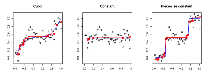
Figure 1: Plots of $Y$ (circles), $\hat{\theta}$ (red), and $\theta^{*}$ (blue) for three different choices of $f$: (i) cubic polynomial (left plot), (ii) constant (middle plot), and (iii) piecewise constant. Here $n=60$, and $\varepsilon\sim N_{n}(0,\sigma^{2}I_{n})$ with $\sigma=0.1$. Here $I_{n}$ denotes the identity matrix of order $n$.

2.1 Worst case risk bound

The worst case risk bound for the isotonic LSE is given by the following inequality. Under the assumption that the errors $\varepsilon_{1},\dots,\varepsilon_{n}$ are i.i.d. with mean zero and variance $\sigma^{2}$, the risk of the isotonic LSE satisfies the bound (see [146]):

$$R(\hat{\theta},\theta^{*})\leq C\left(\frac{\sigma^{2}V(\theta^{*})}{n}\right)^{2/3}+C\frac{\sigma^{2}\log(en)}{n}$$ (12)

where $V(\theta^{*})=\theta_{n}^{*}-\theta_{1}^{*}$ denotes the variation of $\theta^{*}\in\mathcal{I}$ and $C>0$ is a universal constant.

Let us try to understand each of the terms on the right side of (12). As long as the variation $V(\theta^{*})$ is not small the risk $R(\hat{\theta},\theta^{*})$ is given by $(\sigma^{2}V(\theta^{*})/n)^{2/3}$, up to a constant multiplicative factor. This shows that the rate of estimating any monotone function (under the $\ell_{2}$-loss) is $n^{-2/3}$. Moreover, (12) gives the explicit dependence of the risk on the variation of $\theta^{*}$ (and on $\sigma^{2}$).

The second term on the right side of (12) is also interesting — when $V(\theta^{*})=0$, i.e., $\theta^{*}$ is a constant sequence, (12) shows that the risk of the isotonic LSE scales like $\log n/n$. This is a consequence of the fact that $\hat{\theta}$ chooses its blocks (of constancy) adaptively depending on the data. When $\theta^{*}$ is the constant sequence, $\hat{\theta}$ has fewer blocks (in fact, it has of the order of $\log n$ blocks; see [18, Theorem 3] and [102, Theorem 1]) and some of the blocks will be very large (see e.g., the middle plot of Figure 1), so that averaging the responses within the large blocks would yield a value very close to the grand mean $\bar{Y}=(\sum_{i=1}^{n}y_{i})/n$ (which has risk $\sigma^{2}/n$ in this problem). Thus (12) already illustrates the adaptive nature of the LSE — the risk of the LSE $\hat{\theta}$ changes depending on the “structure” of the true $\theta^{*}$. In the next subsection (see (13)) we further highlight this adaptive nature of the LSE.

Remark 2.1.

To the best of our knowledge, inequality (12) first appeared in [102, Theorem 1] who proved it under the assumption that the errors $\varepsilon_{1},\dots,\varepsilon_{n}$ are i.i.d. $N(0,\sigma^{2})$. Zhang [146] proved (12) for much more general errors including the case when $\varepsilon_{1},\dots,\varepsilon_{n}$ are i.i.d. with mean zero and variance $\sigma^{2}$. The proof we give (in Section A.2 of Appendix A) follows the arguments of [146]. Another proof of an inequality similar to (12) for the case of normal errors has been given recently by [26] who proved it as an illustration of a general technique for bounding the risk of LSEs.

Remark 2.2.

The LSE over bounded monotone functions also satisfies the bound (12) and has been observed by many authors including [109, 135, 39]. Proving this result is easier, however, because of the presence of the uniform bound on the function class (such a bound is not present for the isotonic LSE). It must also be kept in mind that the bounded isotonic LSE comes with a tuning parameter that needs to chosen by the user.

Remark 2.3.

Inequality (12) also implies that the isotonic LSE achieves the risk $(\sigma^{2}V/n)^{2/3}$ for $\theta^{*}\in\mathcal{I}_{V}:=\{\theta\in\mathcal{I}:\theta_{n}-\theta_{1}\leq V\}$ (as long as $V$ is not too small) without any knowledge of $V$. It turns out that the minimax risk over $\mathcal{I}_{V}$ is of the order $(\sigma^{2}V/n)^{2/3}$ as long as $V$ is in the range $\sigma/\sqrt{n}\lesssim V\lesssim\sigma n$ (see e.g., [28, Theorem 5.3]). Therefore, in this wide range of $V$, the isotonic LSE is minimax (up to constant multiplicative factors) over the class $\mathcal{I}_{V}$. This is especially interesting because the isotonic LSE does not require any knowledge of $V$. This illustrates another kind of adaptation of the isotonic LSE; further details on this can be found in [31].

2.2 Adaptive risk bounds

As the isotonic LSE fit is piecewise constant, it may be reasonable to expect that when $\theta^{*}$ is itself a piecewise constant (with not too many pieces), the risk of $\hat{\theta}$ would be small. The rightmost plot of Figure 1 corroborates this intuition. This leads us to our second type of risk bound for the LSE. For $\theta\in\mathcal{I}$, let $k(\theta)\geq 1$ denote the number of constant blocks of $\theta$, i.e., $k(\theta)$ is the integer such that $k(\theta)-1$ is the number of inequalities $\theta_{i}\leq\theta_{i+1}$ that are strict, for $i=1,\ldots,n-1$ (the number of jumps of $\theta$).

Theorem 2.1.

Under the assumption that $\varepsilon_{1},\dots,\varepsilon_{n}$ are i.i.d. with mean zero and variance $\sigma^{2}$ we have

$$R(\hat{\theta},\theta^{*})\leq\inf_{\theta\in\mathcal{I}}\left[\frac{1}{n}\|\theta^{*}-\theta\|^{2}+\frac{4\sigma^{2}k(\theta)}{n}\log\frac{en}{k(\theta)}\right]$$ (13)

for every $\theta^{*}\in\mathbb{R}^{n}$.

Note that $\theta^{*}$ in Theorem 2.1 can be any arbitrary vector in $\mathbb{R}^{n}$ (it is not required that $\theta^{*}\in\mathcal{I}$). An important special case of inequality (13) arises when $\theta^{*}\in\mathcal{I}$ and $\theta$ is taken to be $\theta^{*}$ in order to obtain:

$$R(\hat{\theta},\theta^{*})\leq\frac{4\sigma^{2}k(\theta^{*})}{n}\log\frac{en}{k(\theta^{*})}.$$ (14)

It makes sense to compare (14) with the worst case risk bound (12). Suppose, for example, $\theta_{j}^{*}=\mathbf{1}\{j>n/2\}$ (here $\mathbf{1}$ denotes the indicator function) so that $k(\theta^{*})=2$ and $V(\theta^{*})=1$. Then the risk bound in (12) is essentially $(\sigma^{2}/n)^{2/3}$ while the right side of (14) is $(8\sigma^{2}/n)\log(en/2)$ which is much smaller than $(\sigma^{2}/n)^{2/3}$. More generally, if $\theta^{*}$ is piecewise constant with $k$ blocks then $k(\theta^{*})=k$ so that inequality (14) implies that the risk is given by the parametric rate $k\sigma^{2}/n$ with a logarithmic multiplicative factor of $4\log(en/k)$ — this is a much stronger bound compared to (12) when $k$ is small.

Inequality (14) is an example of an oracle inequality. This is because of the following. Let $\hat{\theta}^{OR}$ denote the oracle piecewise constant estimator of $\theta^{*}$ which estimates $\theta^{*}$ by the mean of $Y$ in each constant block of $\theta^{*}$ (note that $\hat{\theta}^{OR}$ uses knowledge of the locations of the constant blocks of $\theta^{*}$ and hence is an oracle estimator). It is easy to see then that the risk of $\hat{\theta}^{OR}$ is given by

$$R(\hat{\theta}^{OR},\theta^{*})=\frac{\sigma^{2}k(\theta^{*})}{n}.$$

As a result, inequality (14) can be rewritten as

$$R(\hat{\theta},\theta^{*})\leq\left(4\log\frac{en}{k(\theta^{*})}\right)R(\hat{\theta}^{OR},\theta^{*}).$$ (15)

Because this involves a comparison of the risk of the LSE $\hat{\theta}$ with that of the oracle estimator $\hat{\theta}^{OR}$, inequality (14) is referred to as an oracle inequality. Inequality (15) shows that the isotonic LSE, which uses no knowledge of $k(\theta^{*})$ and the positions of the blocks, has essentially the same risk performance as the oracle piecewise constant estimator (up to the multiplicative logarithmic factor $4\log(en/k(\theta^{*}))$). This is indeed remarkable!

For certain piecewise constant vectors $\theta^{*}$ with $k$ blocks, it might be possible to approximate $\theta^{*}$ closely with another piecewise constant vector $\tilde{\theta}$ having $k^{\prime}$ blocks where $k^{\prime}<k$. In such cases, it makes sense to compare the performance of the isotonic estimator $\hat{\theta}$ to the oracle piecewise constant estimator with $k^{\prime}$ blocks. Such a comparison is achieved by inequality (13) which is a stronger inequality than (14). In fact, (13) can actually be viewed as a more general oracle inequality where the behavior of the isotonic LSE is compared with oracle piecewise constant estimators even when $\theta^{*}\notin\mathcal{I}$. We would like to mention here that, in this context, (13) is referred to as a sharp oracle inequality because the leading constant in front of the $\lVert\theta^{*}-\theta\rVert^{2}/n$ term on the right-hand side of (13) is equal to one. We refer to [19] for a detailed explanation of oracle and sharp oracle inequalities.

Based on the discussion above, it should be clear to the reader that the adaptive risk bound (13) complements the worst case bound (12) as it gives much finer information about how well any particular $\theta^{*}$ (depending on its ‘complexity’) can be estimated by the LSE $\hat{\theta}$.

Remark 2.4 (Model misspecification).

As already mentioned, the sharp oracle inequality (13) needs no assumption on $\theta^{*}$ (which can be any arbitrary vector in $\mathbb{R}^{n}$), i.e., the inequality holds true even when $\theta^{*}\notin\mathcal{I}$. See [28, Section 6] for another way of handling model misspecification, where $\hat{\theta}$ is compared with the “closest” element to $\theta^{*}$ in $\mathcal{I}$ (and not $\theta^{*}$).

Remark 2.5.

To the best of our knowledge, an inequality of the form (13) first explicitly appeared in [28, Theorem 3.1] where it was proved that

$$R(\hat{\theta},\theta^{*})\leq 4\inf_{\theta\in\mathcal{I}}\left[\frac{1}{n}\|\theta^{*}-\theta\|^{2}+\frac{4\sigma^{2}k(\theta)}{n}\log\frac{en}{k(\theta)}\right]$$ (16)

under the additional assumption that $\theta^{*}\in\mathcal{I}$. The proof of this inequality given in [28] is based on ideas developed in [146]. Note the additional constant factor of $4$ in the above inequality compared to (13).

Under the stronger assumption $\varepsilon\sim N_{n}(0,\sigma^{2}I_{n})$, Bellec [19, Theorem 3.2] improved (16) and proved that

$$R(\hat{\theta},\theta^{*})\leq\inf_{\theta\in\mathcal{I}}\left[\frac{1}{n}\|\theta^{*}-\theta\|^{2}+\frac{\sigma^{2}k(\theta)}{n}\log\frac{en}{k(\theta)}\right],$$ (17)

for every $\theta^{*}\in\mathbb{R}^{n}$. A sketch of the proof of this inequality is given in Subsection A.3 of Appendix A. A remarkable feature of this bound is that the multiplicative constants involved are all tight, which implies, in particular, that

$$R(\hat{\theta},\theta^{*})\leq\inf_{\theta\in\mathcal{I}}\left[\frac{1}{n}\|\theta^{*}-\theta\|^{2}+C\frac{\sigma^{2}k(\theta)}{n}\log\frac{en}{k(\theta)}\right]$$

cannot hold for every $\theta^{*}$ if $C<1$. This follows from the fact that when $\theta^{*}=(0,0,\dots,0)\in\mathcal{I}$ and $\varepsilon\sim N_{n}(0,\sigma^{2}I_{n})$, the risk $R(\hat{\theta},\theta^{*})$ exactly equals $\sigma^{2}\sum_{j=1}^{n}1/j\asymp\sigma^{2}\log n$; see [19] for an explanation. It must be noted that this implies, in particular, that the logarithmic term in these adaptive risk bounds cannot be removed.

Note that inequality (13) has an additional factor of $4$ compared to (17) on the second term in the right-hand side. This is because the errors $\varepsilon_{1},\dots,\varepsilon_{n}$ can be non-Gaussian in Theorem 2.1.

Remark 2.6.

One may attempt to prove (12) from the adaptive risk bound (13) by approximating arbitrary $\theta^{*}\in\mathcal{I}$ via $\theta\in\mathcal{I}$ with a bound on $k(\theta)$. However, it is likely that such an approach will lead to additional logarithmic terms on the right hand side of (12) (see e.g., [28, Theorem 4.1]).

Remark 2.7.

For some choices of $\theta^{*}\in\mathcal{M}$, it is possible to obtain bounds on the risk $R(\hat{\theta},\theta^{*})$ of the LSE which combine aspects of both (12) and (13). For example, if $\theta^{*}$ is piecewise constant with $k$ blocks for $1\leq i\leq n/2$ and if it is strictly increasing with variation bounded by $V$ for $n/2\leq i\leq n$, then it can be shown that the risk of the LSE will be bounded from above by a constant multiple of $\sigma^{2}(k/n)\log({en}/{k})+(\sigma^{2}V/n)^{2/3}$. Techniques for obtaining such hybrid risk bounds in isotonic regression can be found in [146, Sections 2 and 3].

2.2.1 Adaptive Risk Bounds for $R^{(p)}(\hat{\theta},\theta^{*})$.

The risk bound (13) (or more specifically (15)) implies that the isotonic LSE pays a logarithmic price in risk compared to the oracle piecewise constant estimator. This fact is strongly tied to the fact that the risk is measured via squared error loss (as in (9)). The story will be different if one measures risk under $\ell_{p}$-metrics for $p\neq 2$. To illustrate this, we shall describe adaptive bounds for the risk $R^{(p)}(\hat{\theta},\theta^{*})$ defined in (10).

The following result bounds the risk $R^{(p)}(\hat{\theta},\theta^{*})$ assuming that $\theta^{*}\in\mathcal{I}$. The risk bounds involve a positive constant $C_{p}$ that depends on $p$ alone. Explicit expressions for $C_{p}$ can be gleaned from the proof of Theorem 2.2 (in Section A.5).

Theorem 2.2.

Assume that the errors $\varepsilon_{1},\dots,\varepsilon_{n}$ are i.i.d. $N(0,\sigma^{2})$. Fix $\theta^{*}\in\mathcal{I}$ and let $p\geq 1,p\neq 2$. Let $k$ denote the number of constant blocks of $\theta^{*}$ and let the lengths of the blocks be denoted by $n_{1},\dots,n_{k}$. We then have

$$R^{(p)}(\hat{\theta},\theta^{*})\leq C_{p}\frac{\sigma^{p}}{n}\sum_{i=1}^{k}n_{i}^{(2-p)_{+}/2}\leq C_{p}\sigma^{p}\left(\frac{k}{n}\right)^{\min(p,2)/2}$$ (18)

where $C_{p}$ is a positive constant that depends on $p$ alone.

Remark 2.8.

As stated, Theorem 2.2 appears to be new even though its conclusion is implicit in the detailed risk calculations of [146] for isotonic regression. We have assumed that $\varepsilon_{1},\dots,\varepsilon_{n}$ are normal in Theorem 2.2 but it is possible to allow non-Gaussian errors by imposing suitable moment conditions.

Remark 2.9.

From an examination of the proof of Theorem 2.2 (given in Subsection A.5), it is evident that the constant $C_{p}$ tends to $+\infty$ as $p\rightarrow 2$. Note that this makes sense because when $p=2$, the right hand side of (18) equals $C_{p}\sigma^{2}k/n$ and we know from the previous subsection that there must be a logarithmic term (in $n$) for the risk when $p=2$. It is helpful here to note that by Jensen’s inequality (and the bound (14)), we have, for $1\leq p\leq 2$, the bound

$$R^{(p)}(\hat{\theta},\theta^{*})\leq\left(R^{(2)}(\hat{\theta},\theta^{*})\right)^{p/2}\leq 4^{p/2}\sigma^{p}\left(\frac{k}{n}\right)^{p/2}\left(\log\frac{en}{k}\right)^{p/2}.$$

which does not explode as $p\uparrow 2$. The above bound can also be obtained by modifying the proof of Theorem 2.2 where in place of the inequality

$$\sum_{j=1}^{n}j^{-p/2}\leq\frac{2}{2-p}n^{1-(p/2)}\qquad\text{for $1\leq p<2$},$$ (19)

we use

$$\sum_{j=1}^{n}j^{-p/2}\leq n\left(\frac{1}{n}\sum_{j=1}^{n}\frac{1}{j}\right)^{p/2}\leq n\left(\frac{\log(en)}{n}\right)^{p/2}\qquad\text{for all $1\leq p\leq 2$}$$ (20)

which is again a consequence of Jensen’s inequality.

Let us now compare the isotonic LSE to the oracle piecewise constant estimator $\hat{\theta}^{OR}$ (introduced in the previous subsection) in terms of the $\ell_{p}$-risk. It is easy to verify that the risk of $\hat{\theta}^{OR}$ under the $\ell_{p}$-loss is given by

$$R^{(p)}(\hat{\theta}^{OR},\theta^{*})=(\mathbb{E}|\eta|^{p})\sigma^{p}\frac{1}{n}\sum_{i=1}^{k}n_{i}^{(2-p)/2}$$ (21)

for every $p>0$ where $\eta:=\varepsilon_{1}/\sigma$ is standard normal.

Comparing (18) and (21), we see that the isotonic LSE performs at the same rate (up to constant multiplicative factors) as the oracle piecewise constant estimator for $1\leq p<2$ (there is not even a logarithmic price for these values of $p$). When $p=2$, as seen from (15), the isotonic LSE pays a logarithmic price of $4\log(en/k(\theta^{*}))$. For $p>2$ however, there is a significant price that is paid. For example, if all the constant blocks have roughly equal size, then the oracle estimator’s risk, when $p>2$, is of order $(k/n)^{p/2}$ while the bound in (18) is of order $k/n$. It is also actually true that if $\mathcal{I}_{k}$ denotes the class of all $\theta^{*}\in\mathcal{I}$ with $k$ constant blocks, then (for a positive constant $C_{p}$)

$$\sup_{\theta^{*}\in\mathcal{I}_{k}}R^{(p)}(\hat{\theta},\theta^{*})\geq C_{p}\sigma^{p}\left(\frac{k}{n}\right)\qquad\text{for every $p>2$}$$ (22)

and this confirms the fact that there is a significant price to be paid by the LSE (compared to the oracle piecewise constant estimator) for estimating $\theta^{*}\in\mathcal{I}_{k}$ when the risk is measured by $R^{(p)}(\hat{\theta},\theta^{*})$ for $p>2$. A sketch of the proof of (22) is given in Subsection A.4.

Theorem 2.2 can be generalized to situations where $\theta^{*}\in\mathcal{I}$ has a large number of constant blocks provided it can be well-approximated by $\theta\in\mathcal{I}$ with a small (compared to $n$) number of constant blocks. This result is given below (and proved in Subsection A.6). It is similar in spirit to (13) even though it is not as sharp or clean as (13). We need some notation to state this result. An interval partition $\pi$ of $n$ is a finite sequence of positive integers that sum to $n$. Let $\Pi$ denote the set of all such interval partitions $\pi$ of $n$. For each $\pi=(n_{1},\dots,n_{k})\in\Pi$, let $k(\pi):=k$. The variation of $\theta\in\mathcal{I}$ with respect to $\pi\in\Pi$ is defined as

$$V_{\pi}(\theta):=\max_{1\leq i\leq k}\left(\theta_{s_{i}}-\theta_{s_{i-1}}\right)$$

where $s_{i},0\leq i\leq k$ are defined (with respect to the partition $\pi:=(n_{1},\dots,n_{k})$) as $s_{0}:=0$ and $s_{i}:=n_{1}+\dots+n_{i}$ for $i=1,\dots,k$.

Theorem 2.3.

Assume that the errors $\epsilon_{1},\dots,\epsilon_{n}$ are i.i.d $N(0,\sigma^{2})$. Fix $\theta^{*}\in\mathcal{I}$ and let $p\geq 1,p\neq 2$. Then

$$R^{(p)}(\hat{\theta},\theta^{*})\leq C_{p}\inf_{\pi\in\Pi}\left(\left[V_{\pi}(\theta^{*})\right]^{p}+\sigma^{p}\left(\frac{k(\pi)}{n}\right)^{\min(p,2)/2}\right)$$ (23)

for a positive constant $C_{p}$ that depends on $p$ alone.

Unlike (13), inequality (23) is not a sharp oracle inequality because it only holds for $\theta^{*}\in\mathcal{I}$ (and not for general $\theta^{*}\in\mathbb{R}^{n}$) and because the constant in front of the $V_{\pi}(\theta^{*})$ term is not one. However it is still useful and it includes Theorem 2.2 as a special case (indeed to derive (18) from (23), just take the partition $\pi$ which corresponds to the constant blocks of $\theta^{*}$). The bound (23) can also be used to obtain worst case risk bounds for the LSE in terms of the $L^{p}$ risk for $1\leq p<2$ (analogous to (12)). Indeed, it can be shown (see, for example, [28, Lemma 11.1 in the supplementary material]) that for every $\theta^{*}\in\mathcal{I}$ and $\delta>0$, there exists $\pi\in\Pi$ with

$$V_{\pi}(\theta^{*})\leq\delta~{}~{}\text{ and }~{}~{}k(\pi)\leq 1+\frac{V(\theta^{*})}{\delta}.$$

This implies from (23) that

$$R^{(p)}(\hat{\theta},\theta^{*})\leq C_{p}\inf_{\delta>0}\left(\delta^{p}+\sigma^{p}\left(\frac{1}{n}+\frac{V(\theta^{*})}{n\delta}\right)^{\min(p,2)/2}\right).$$

From here, it can be shown that

$$R^{(p)}(\hat{\theta},\theta^{*})\leq C_{p}\left(\frac{\sigma^{2}V(\theta^{*})}{n}\right)^{p/3}+C_{p}\left(\frac{\sigma^{2}}{n}\right)^{p/2}\qquad\text{for $1\leq p<2$}.$$

It turns out that this bound cannot be improved (up to the multiplicative factor $C_{p}$) as argued in [146, Theorem 2.2 and the following discussion]. We would like to remark here that this method will lead to a suboptimal worst case risk bound for $R^{(p)}(\hat{\theta},\theta^{*})$ for $p>2$.

3 Risk bounds in other shape-restricted regression problems

In this section we consider the problems of convex regression (Example 1.3), isotonic regression on a partially ordered set (Example 1.2), unimodal regression (Example 1.4) and shape restricted additive models (Example 1.5). In each of these problems, we describe results related to the performance of the LSEs. The reader will notice that the risk results are not as detailed as compared to the isotonic regression results of the previous section.

3.1 Convex Regression

Let us consider Example 1.3 where the goal is to estimate a convex function $f:[0,1]\to\mathbb{R}$ from regression data as in (1). The convex LSE $\hat{\theta}$ is defined as the projection of $Y$ onto the closed convex cone $\mathcal{K}$ (see (6)). This estimator was first proposed in [73] for the estimation of production functions and Engel curves. It can be shown that $\hat{\theta}$ is piecewise affine with knots only at the design points; see [62, Lemma 2.6]. The accuracy of the LSE, in terms of the risk $R(\hat{\theta},\theta^{*})$ (defined in (9)), was first studied in [68] followed by [28, 19, 27]. These results are summarized below. Earlier results on the risk under a supremum loss can be found in [70, 43].

Suppose that $\varepsilon\sim N_{n}(0,\sigma^{2}I_{n})$. In [27], the following worst case risk bound for $\hat{\theta}$ was given (when $x_{i}=i/n$ are the ordered design points):

$$R(\hat{\theta},\theta^{*})\leq C\left(\frac{\sigma^{2}\sqrt{T(\theta^{*})}}{n}\right)^{4/5}+C\frac{\sigma^{2}}{n^{4/5}}$$ (24)

where $C>0$ is a universal constant and $T(\theta^{*})$ is a constant depending on $\theta^{*}$ (like $V(\theta^{*})$ in (12) for isotonic regression). Roughly speaking, $T(\theta^{*})$ measures the “distance” of $\theta^{*}$ from the set of all affine (functions) sequences. Formally, Let $L$ denote the subspace of $\mathbb{R}^{n}$ spanned by the constant vector $(1,\ldots,1)$ and the vector $(1,2,\ldots,n)$; i.e., $L$ is the linear subspace of affine sequences. Let $P_{L}$ denote the orthogonal projection matrix onto the subspace $L$ and let $\beta^{*}:=(I_{n}-P_{L})\theta^{*}$. Then $T(\theta^{*}):=\max_{1\leq i\leq n}\beta_{i}^{*}-\min_{1\leq i\leq n}\beta_{i}^{*}$. Observe that when $\theta^{*}$ itself is an affine sequence (which is also a convex sequence), then $T(\theta^{*})=0$.

The risk bound (24) shows that the risk of the convex LSE is bounded above by $n^{-4/5}$. Inequality (24) improved a result in [68], which had a similar bound but with an additional multiplicative logarithmic factor (in $n$). Comparing with (12), it is natural to conjecture that the second term in (24) can be improved to $C\sigma^{2}(\log(en))/n$ but this has not been proved so far. Another feature of (24) is that the errors are assumed to be Gaussian; it might be possible to extend them to sub-Gaussian errors but this is still a strong assumption compared to the corresponding result for isotonic regression (see (12)) which holds without distributional assumptions.

The proof of (24) (and other worst case risk bounds like (24) for shape-restricted regression problems under Gaussian/sub-Gaussian errors) involves tools from the theory of Gaussian processes like chaining and Dudley’s entropy bound and crucially relies on an accurate ‘size’ measure of the underlying class (e.g., ‘local’ balls of $\mathcal{K}$) as captured by its metric entropy; see Section 3.5 for a broad outline of the proof strategy. Although the main idea of the proof is simple, deriving appropriate bounds on the metric entropy of the underlying class can be challenging.

As with the isotonic LSE, the convex LSE $\hat{\theta}$ exhibits adaptive behavior. As the convex LSE $\hat{\theta}$ is piecewise affine it may be expected that the risk of $\hat{\theta}$ would be nearly parametric if the true $\theta^{*}$ is (well approximated by) a piecewise affine function. Indeed this is the case. For $\theta\in\mathcal{K}$ let $q(\theta)\geq 1$ denote the number of affine pieces of $\theta$; i.e., $q(\theta)$ is an integer such that $q(\theta)-1$ is the number of inequalities in (6) that are strict. This adaptive behavior can be illustrated through the following risk bound:

$$R(\hat{\theta},\theta^{*})\leq\inf_{\theta\in\mathcal{K}}\left[\frac{1}{n}\|\theta^{*}-\theta\|^{2}+\frac{8\sigma^{2}q(\theta)}{n}\log\frac{en}{q(\theta)}\right].$$ (25)

This inequality has been proved by [19, Section 4] improving earlier results of [68, 28] which had superfluous multiplicative constants. Note that this bound holds for $\varepsilon\sim N(0,\sigma^{2}I_{n})$. It is not known if the bounds holds for non-Gaussian errors (compare this with the corresponding inequality (13) for isotonic regression which holds without distributional assumptions on the errors). Let us also note that risk bounds for the LSE under the $R^{(p)}(\hat{\theta},\theta^{*})$ risk (defined in (10)) are not available for convex regression.

3.2 Isotonic regression on a partially ordered set

We now turn our attention to Example 1.2 where the covariates are partially ordered and the goal is to estimate the order preserving (isotonic) regression function. The book Robertson et al. [118, Chapter 1] gives a nice overview of the characterization and computation of LSEs in such problems along with their applications in statistics. However, not much is known in terms of rates of convergence for these LSEs beyond the example of coordinate-wise nondecreasing ordering introduced in Example 1.2.

In this subsection we briefly review the main results in [29] which considers estimation of a bivariate ($d=2$) coordinate-wise nondecreasing regression function. An interesting recent paper [69] has extended these results to all dimensions $d\geq 2$ (see Remark 3.1). Estimation of bivariate coordinate-wise nondecreasing functions has applications and connections to the problem of estimating matrices of pairwise comparison probabilities arising from pairwise comparison data ([32, 126]) and to seriation ([47]).

As the distribution of the design points $x_{i}$ complicate the analysis of shape-restricted LSEs, especially when $d>1$, for simplicity, we consider the regular uniform grid design. This reduces the problem to estimating an isotonic ‘matrix’ $\theta^{*}:=(\theta_{ij}^{*})\in\mathbb{R}^{n_{1}\times n_{2}}$ from observations

$${y}_{ij}=\theta_{ij}^{*}+\varepsilon_{ij},\qquad\mbox{for }i=1,\ldots,n_{1},\;j=1,\ldots,n_{2},$$

where $\theta^{*}$ is constrained to lie in

$$\mathcal{M}:=\{\theta\in\mathbb{R}^{n_{1}\times n_{2}}:\theta_{ij}\leq\theta_{kl}\mbox{ whenever $i\leq k$ and $j\leq l$}\},$$

and the random errors $\varepsilon_{ij}$’s are i.i.d. $N(0,\sigma^{2})$, with $\sigma^{2}>0$ unknown. We refer to any matrix in $\mathcal{M}$ as an isotonic matrix. Letting $Y:=({y}_{ij})$ denote the matrix (of order $n_{1}\times n_{2}$; $n:=n_{1}n_{2}$) of the observed responses, the LSE $\hat{\theta}$ is defined as the minimizer of the squared Frobenius norm, $\|Y-\theta\|^{2}$, over $\theta\in\mathcal{M}$, i.e.,

$$\hat{\theta}:=\operatorname*{arg\,min}_{\theta\in\mathcal{M}}\sum_{i=1}^{n_{1}}\sum_{j=1}^{n_{2}}({y}_{ij}-\theta_{ij})^{2}.$$ (26)

As $\mathcal{M}$ is a closed convex cone in $\mathbb{R}^{n_{1}\times n_{2}}$, the LSE $\hat{\theta}$ exists uniquely.

The goal now is to formulate both the worst case and adaptive risk bounds for the matrix isotonic LSE $\hat{\theta}$ in estimating $\theta^{*}$. In [29, Theorem 2.1] it was shown that

$$R(\hat{\theta},\theta^{*})\leq C\left(\sqrt{\frac{\sigma^{2}V^{2}(\theta^{*})}{n}}(\log n)^{4}+\frac{\sigma^{2}}{n}(\log n)^{8}\right)$$ (27)

for a universal constant $C>0$, where $V(\theta^{*}):=\theta_{n_{1}n_{2}}^{*}-\theta_{11}^{*}$ is the variation of the isotonic matrix $\theta^{*}$. The above bound shows that when the variation $V(\theta^{*})$ of $\theta^{*}$ is a non-zero constant, the risk of $\hat{\theta}$ decays at the rate $n^{-1/2}$, while when $V(\theta^{*})=0$ (i.e., $\theta^{*}$ is a constant), the risk is (almost) parametric. The above bound probably has superfluous logarithmic factors but bounds with smaller logarithmic factors have not yet been proved. Some understanding of the dependence of the bound (27) on $\sigma,V(\theta^{*})$ and $n$ (which is different from the corresponding dependence in the one dimensional bound (12)) can be derived from the following scaling argument. The risk $R(\hat{\theta},\theta^{*})$ only depends on $\theta^{*}$ and $\sigma$ so let us denote it by $g(\theta^{*},\sigma)$. By a natural scaling argument (where we multiply all the observations by a constant $t>0$), it should be clear that

$$g(\theta^{*},\sigma)=t^{2}g(\theta^{*}/t,\sigma/t)\qquad\text{for every $t>0$}.$$ (28)

It is easy to see now that the same identity holds when $g(\theta^{*},\sigma)$ is taken to be the right hand side of (27) as well. This will not be true if, for example, $V^{2}(\theta^{*})$ is replaced by some other power of $V(\theta^{*})$ in the right hand side of (27). This argument, via the scaling identity (28), can be used to understand the dependencies on $\theta^{*}$ and $n$ in the one-dimensional bound (12) as well.

To describe the adaptive risk bound for the matrix isotonic LSE we need to introduce some notation. A subset $A$ of $\{1,\dots,n_{1}\}\times\{1,\dots,n_{2}\}$ is called a rectangle if $A=\{(i,j):k_{1}\leq i\leq l_{1},k_{2}\leq j\leq l_{2}\}$ for some $1\leq k_{1}\leq l_{1}\leq n_{1}$ and $1\leq k_{2}\leq l_{2}\leq n_{2}$. A rectangular partition of $\{1,\dots,n_{1}\}\times\{1,\dots,n_{2}\}$ is a collection of rectangles $\pi=(A_{1},\dots,A_{k})$ that are disjoint and whose union is $\{1,\dots,n_{1}\}\times\{1,\dots,n_{2}\}$. The cardinality of such a partition, $|\pi|$, is the number of rectangles in the partition. The collection of all rectangular partitions of $\{1,\dots,n_{1}\}\times\{1,\dots,n_{2}\}$ will be denoted by ${\mathcal{P}}$. For $\theta\in\mathcal{M}$ and $\pi=(A_{1},\dots,A_{k})\in{\mathcal{P}}$, we say that $\theta$ is constant on $\pi$ if $\{\theta_{ij}:(i,j)\in A_{l}\}$ is a singleton for each $l=1,\dots,k$. We define $k(\theta)$, for $\theta\in\mathcal{M}$, as the “number of rectangular blocks” of $\theta$, i.e., the smallest integer $k$ for which there exists a partition $\pi\in{\mathcal{P}}$ with $|\pi|=k$ such that $\theta$ is constant on $\pi$. In [29, Theorem 2.4] the following adaptive risk bound was stated:

$$R(\hat{\theta},\theta^{*})\leq\inf_{\theta\in\mathcal{M}}\left(\frac{\|\theta^{*}-\theta\|^{2}}{n}+\frac{C\sigma^{2}k(\theta)}{n}(\log n)^{8}\right).$$ (29)

where $C>0$ is a universal constant.

In [29] the authors also established a property of the LSE that they termed ‘variable’ adaptation. Let $\mathcal{I}_{n_{1}}:=\left\{\theta\in\mathbb{R}^{n_{1}}:\theta_{1}\leq\dots\leq\theta_{n_{1}}\right\}$. Suppose $\theta^{*}=(\theta^{*}_{ij})\in\mathcal{I}$ has the property that $\theta^{*}_{ij}$ only depends on $i$, i.e., there exists $\theta^{**}\in\mathcal{I}_{n_{1}}$ such that $\theta^{*}_{ij}=\theta^{**}_{i}$ for every $i$ and $j$. If we knew this fact about $\theta^{*}$, then the most natural way of estimating it would be to perform vector isotonic estimation based on the row-averages $\bar{y}:=\left(\bar{y}_{1},\dots,\bar{y}_{n_{1}}\right)$, where $\bar{y}_{i}:=\sum_{j=1}^{n_{2}}y_{ij}/n_{2}$, resulting in an estimator $\breve{\theta}$ of $\theta^{**}$. Note that the construction of $\breve{\theta}$ requires the knowledge that all rows of $\theta^{*}$ are constant. As a consequence of the adaptive risk bound (29), it was shown in [29, Theorem 2.4] that the matrix isotonic LSE $\hat{\theta}$ achieves the same risk bounds as $\breve{\theta}$, up to additional logarithmic factors. This is remarkable because $\hat{\theta}$ uses no special knowledge on $\theta^{*}$; it automatically adapts to intrinsic dimension of $\theta^{*}$.

Remark 3.1 (Extension to $d\geq 2$).

The recent paper, Han et al. [69], studied $d$-dimensional isotonic regression for general $d\geq 1$ and proved versions of inequalities (27) and (29). Specifically, it is shown there that the worst case risk of the LSE is bounded from above by $n^{-1/d}(\log n)^{4}$ (ignoring multiplicative factors involving $\sigma$ and $V(\theta^{*})$). Note that for $d=2$, this matches the rate given by (27). Interestingly, it is also shown in [69] that the LSE is minimax rate optimal (up to the $(\log n)^{4}$ factor) over the class of all bounded isotonic functions. This minimax optimality of the LSE is especially impressive because the class of all bounded isotonic functions for $d\geq 3$ is quite massive in terms of metric entropy and it was suspected previously that the LSE might suffer from overfitting. [69] also extended the adaptive risk bound (29) to $d\geq 3$ by proving that

$$R(\hat{\theta},\theta^{*})\leq\inf_{\theta\in\mathcal{M}}\left(\frac{\|\theta^{*}-\theta\|^{2}}{n}+C_{d}\sigma^{2}\left(\frac{k(\theta)}{n}\right)^{2/d}(\log n)^{8}\right).$$

Note that the $k(\theta)/n$ term in (29) is replaced by $(k(\theta)/n)^{2/d}$ in the above bound. [69, Proposition 2] also observed that the above bound will not hold if $(k(\theta)/n)^{2/d}$ is replaced by $k(\theta)/n$. This implies that the LSE for $d\geq 3$ also displays adaptive behavior for piecewise hyperrectangular constant functions but that the adaptation risks are not parametric. We should also mention here that [69] also obtained results for the isotonic LSE under random design settings.

Let us reiterate that the bounds (27) and (29) are established under the assumption that the errors $\varepsilon_{i,j}$ are i.i.d. $N(0,\sigma^{2})$. It is possible to generalize them to sub-Gaussian errors (see [19, Section 6] for general results with sub-Gaussian errors). However, it is not known if they hold under general error distributions that are not sub-Gaussian. Also risk bounds in other loss functions (such as those in appropriate $\ell_{p}$-metrics) are not available.

3.3 Unimodal Regression

In this subsection we summarize the two kinds of risk bounds known for the LSE in unimodal (decreasing and then increasing) regression, introduced in Example 1.4. The unimodal LSE $\hat{\theta}$ is defined as any projection of $Y$ onto $\mathcal{U}$, a finite union of the closed convex cones described in Example 1.4. It is known that $\hat{\theta}$ is piecewise constant with possible jumps only at the design points. Once the mode of the fitted LSE is known (and fixed), $\hat{\theta}$ is just the nonincreasing (isotonic) LSE fitted to the points to the left of the mode and nondecreasing (isotonic) LSE fitted to the points on the right of the mode.

As in isotonic regression, the unimodal LSE $\hat{\theta}$ exhibits adaptive behavior. In fact, the risk bounds for the unimodal LSE $\hat{\theta}$ are quite similar to those obtained for the isotonic LSE. The two kinds of risk bounds are given below (under the assumption that $\varepsilon\sim N_{n}(0,\sigma^{2}I_{n})$):

$$R(\hat{\theta},\theta^{*})\leq C\left(\frac{\sigma^{2}V(\theta^{*})}{n}\right)^{2/3}+C\frac{\sigma^{2}}{n^{2/3}},\quad\mbox{where }\theta^{*}\in\mathcal{U},$$ (30)

and

$$R(\hat{\theta},\theta^{*})\leq C\inf_{\theta\in\mathcal{U}}\left[\frac{1}{n}\|\theta^{*}-\theta\|^{2}+C\frac{\sigma^{2}(k(\theta)+1)}{n}\log\frac{en}{k(\theta)+1}\right]$$ (31)

where $k(\theta)$ is the number of constant blocks of $\theta$, $V(\theta^{*}):=\max_{i,j}|\theta_{i}^{*}-\theta_{j}^{*}|$ is the range or variation of $\theta^{*}$ and $C>0$ is a universal constant.

The worst case risk bound (30) is given in [30, Theorem 2.1] while the adaptive risk bound (31) is a consequence of [19, Theorem A.4] (after integrating the tail probability). The proof of (30) (given in [30, Theorem 2.1]) is based on the general theory of least squares outlined in Section 3.5; also see [26, Theorem 2.2]. It shows that a unimodal regression function can also be estimated at the same rate as a monotone function. The adaptive risk bound (31), although being similar in spirit to that of the isotonic LSE, is weaker than (17) (obtained for the isotonic LSE). Note that inequality (31) is not sharp (i.e., the leading constant on the right side of (31) is not 1); in fact it is not known whether a sharp oracle inequality can be constructed for $R(\hat{\theta},\theta^{*})$ (see [19]). The proof of the adaptive risk bound is also slightly more involved than that of Theorem 2.1; the fact that the underlying parameter space $\mathcal{U}$ is non-convex complicates the analysis.

3.4 Shape-restricted additive models

Given observations $(x_{1},y_{1}),\dots,(x_{n},y_{n})$ where $\{x_{i}=(x_{ij},1\leq j\leq d)\}_{i=1}^{n}$ are $d$-dimensional design points and $y_{1},\dots,y_{n}$ are real-valued, the additive model (see e.g., [72, 95]) assumes that

$$y_{i}=\mu^{*}+\sum_{j=1}^{d}f^{*}_{j}(x_{ij})+\varepsilon_{i}\qquad\text{for $i=1,\dots,n$}$$

where $\mu^{*}\in\mathbb{R}$ is an unknown intercept term, $f^{*}_{1},\dots,f^{*}_{d}$ are unknown univariate functions satisfying

$$\frac{1}{n}\sum_{i=1}^{n}f^{*}_{j}(x_{ij})=0,\quad\mbox{ for every }j=1,\dots,d,$$ (32)

and $\varepsilon_{1},\ldots,\varepsilon_{n}$ are unobserved mean-zero errors. An assumption similar to (32) is necessary to ensure the identifiability of $f^{*}_{1},\dots,f^{*}_{d}$. We focus our attention to shape-restricted additive models where it is assumed that each $f^{*}_{j}$ obeys a known qualitative restriction such as monotonicity or convexity which is captured by the assumption that $f^{*}_{j}\in\mathcal{F}_{j}$ for a known class of functions $\mathcal{F}_{j}$. One of the main goals in additive modeling is to recover each individual function $f^{*}_{j}\in\mathcal{F}_{j}$ for $j=1,\dots,d$.

The LSEs $\hat{\mu},\hat{f}_{j}$ of $\mu^{*},f_{j}^{*}$, for $j=1,\dots,d$ are defined as minimizers of the sum of squares criterion, i.e.,

$$(\hat{\mu},\hat{f}_{1},\ldots,\hat{f}_{d}):=\operatorname*{arg\,min}\sum_{i=1}^{n}\Big{(}y_{i}-\mu-\sum_{j=1}^{d}f_{j}(x_{ij})\Big{)}^{2}$$ (33)

under the constraints $\mu\in\mathbb{R},f_{j}\in\mathcal{F}_{j},\sum_{i=1}^{n}f_{j}(x_{ij})=0\text{ for }j=1,\dots,d.$ It is natural to compare the performance of these LSEs to the corresponding oracle estimators defined in the following way. For each $k=1,\dots,d$, the oracle estimator $\hat{f}^{OR}_{k}$ is defined as

$$\hat{f}^{OR}_{k}:=\operatorname*{arg\,min}_{f_{k}}\sum_{i=1}^{n}\Big{(}y_{i}-\mu^{*}-\sum_{j\neq k}f^{*}_{j}(x_{ij})-f_{k}(x_{ik})\Big{)}^{2},$$ (34)

where $f_{k}\in\mathcal{F}_{k}$ and satisfies $\sum_{i=1}^{n}f_{k}(x_{ik})=0$. In other words, $\hat{f}_{k}^{OR}$ assumes knowledge of $f^{*}_{j}$, for $j\neq k$, and $\mu^{*}$, and performs least squares minimization only over $f_{k}\in\mathcal{F}_{k}$.

A very important aspect about shape-restricted additive models is that it is possible for the LSE $\hat{f}_{k}$ to be close to the oracle estimator $\hat{f}^{OR}_{k}$, for each $k=1,\dots,d$. Indeed, this property was proved by Mammen and Yu [98] under certain assumptions for additive isotonic regression where each function $f_{j}$ is assumed to be monotone. Specifically, [98] worked with a random design setting where the design points are assumed to be i.i.d. from a Lipschitz density that is bounded away from zero and infinity on $[0,1]^{d}$ (this is a very general setting which allows for non-product measures). They also assumed that each function $f_{j}$ is differentiable and strictly increasing. Although the design restrictions in this result are surprisingly minimal, we believe that the assumptions on the $f_{j}$’s can be relaxed. In particular, this result should hold when $f_{j}$’s are piecewise constant and even under more general shape restrictions such as convexity.

Our intuition is based on the following simple observation that there exist design configurations where the LSE $\hat{f}_{k}$ is remarkably close to $\hat{f}^{OR}_{k}$ for each $k=1,\dots,d$ under almost no additional assumptions. The simplest such instance is when the set of design points $\mathcal{X}:=\{x_{1},\dots,x_{n}\}\subseteq\mathbb{R}^{d}$ has a Cartesian product structure in the sense that $\mathcal{X}$ equals $\mathcal{X}_{1}\times\dots\times\mathcal{X}_{d}$ where each $\mathcal{X}_{i}$ is a subset of the real line. In this case, it is easy to see that $\hat{f}_{k}$ is exactly equal to $\hat{f}^{OR}_{k}$ as stated in the result below. It is convenient here to index the observations as $(i_{1},\dots,i_{d})$ where each $i_{j}$ ranges in the set $\mathcal{X}_{j}$ for $j=1,\dots,d$. The observation model can then be written as

$$y_{i_{1},i_{2},\dots,i_{d}}=\mu^{*}+f_{1}^{*}(i_{1})+f_{2}^{*}(i_{2})+\dots+f_{d}^{*}(i_{d})+\varepsilon_{i_{1},i_{2},\dots,i_{d}},$$ (35)

for $i_{n}\in\mathcal{X}_{j},j=1,\dots,d$. The following result is proved in Section A.7 for the special case $d=2$ (the proof for the general case follows analogously).

Lemma 3.1.

Consider model (35) where $f_{j}^{*}\in\mathcal{F}_{j}$, for $j=1,\dots,d$. Suppose that $\hat{f}_{j},j=1,\dots,d$ denote the LSEs of $f_{j}^{*},j=1,\dots,d$, as defined in (33). Also, let the oracle estimators $\hat{f}_{j}^{OR},j=1,\dots,d$ be as defined in (34). Then $\hat{f}_{j}=\hat{f}_{j}^{OR}$ for every $j=1,\dots,d$.

Note that we have made no assumptions at all on $\mathcal{F}_{1},\dots,\mathcal{F}_{d}$. Thus when the design points come from a product set $\mathcal{X}_{1}\times\dots\times\mathcal{X}_{d}$ in $\mathbb{R}^{d}$, the LSE of $f^{*}_{j}$ is exactly equal to the oracle estimate $\hat{f}_{j}^{OR}$ for every $j=1,\dots,d$. For general design configurations, it might be much harder to relate the LSEs to the corresponding oracle estimators. Nevertheless, the aforementioned phenomenon for gridded designs allows us to conjecture that the closeness of $\hat{f}_{j}$ to $\hat{f}_{j}^{OR}$ must hold in much greater generality than has been observed previously in the literature.

It may be noted that the risk behavior of $\hat{f}_{j}^{OR}$ is easy to characterize. For example, when $f_{j}^{*}$ is assumed to be monotone, $\hat{f}_{j}^{OR}$ will satisfy risk bounds similar to those described in Section 2. Likewise, when $f_{j}^{*}$ is assumed to be convex, then $\hat{f}_{j}^{OR}$ will satisfy risk bounds described in Subsection 3.1. Thus, when $\hat{f}_{j}$ is close to $\hat{f}_{j}^{OR}$ (which we expect to happen under a broad set of design configurations), it is natural to expect that $\hat{f}_{j}$ will satisfy such risk bounds as well.

3.5 General theory of LSEs

In this section, we collect some general results on the behavior of the LSEs that are useful for proving the risk bounds described in the previous two sections. These results apply to LSEs that are defined by (7) for a closed convex constraint set $\mathcal{C}$. Convexity of $\mathcal{C}$ is crucial here (in particular, these results do not directly apply to unimodal regression where the constraint set is non-convex; see Section 3.3). We assume that the observation vector $Y=\theta^{*}+\varepsilon$ for a mean-zero random vector $\varepsilon$. Except in Lemma 3.4, we assume that $\varepsilon\sim N_{n}(0,\sigma^{2}I_{n})$.

The first result reduces the problem of bounding $R(\hat{\theta},\theta^{*})$ to controlling the expected supremum of an appropriate Gaussian process. This result was proved by Chatterjee [26] (see [33, 136] for extensions to penalized LSEs).

Lemma 3.2 (Chatterjee).

Consider the LSE (7) for a fixed closed convex set $\mathcal{C}$. Assume that $Y=\theta^{*}+\varepsilon$ where $\varepsilon\sim N_{n}(0,\sigma^{2}I_{n})$ and $\theta^{*}\in\mathcal{C}$. Let us define the function $g_{\theta^{*}}:\mathbb{R}_{+}\rightarrow\mathbb{R}$ as

$$g_{\theta^{*}}(t):=\mathbb{E}\left[\sup_{\theta\in\mathcal{C}:\|\theta-\theta^{*}\|\leq t}\langle\varepsilon,\theta-\theta^{*}\rangle\right]-\frac{t^{2}}{2}.$$ (36)

Let $t_{\theta^{*}}$ be the point in $[0,\infty)$ where $t\mapsto g_{\theta^{*}}(t)$ attains its maximum (existence and uniqueness of $t_{\theta^{*}}$ are proved in [26, Theorem 1.1]). Then there exists a universal positive constant $C$ such that

$$R(\hat{\theta},\theta^{*})\leq\frac{C}{n}\max\left(t_{\theta^{*}}^{2},\sigma^{2}\right).$$ (37)

Remark 3.2.

Chatterjee [26] actually proved a result that is much stronger than (37). Specifically, he proved that the fluctuations of the random variable $\|\hat{\theta}-\theta^{*}\|$ around the deterministic quantity $t_{\theta^{*}}$ are of the order $\sqrt{t_{\theta^{*}}}$. When $t_{\theta^{*}}$ is large, this therefore implies that $\|\hat{\theta}-\theta^{*}\|$ is tightly concentrated around $t_{\theta^{*}}$. The bound (37) is an easy consequence of this concentration result.

Lemma 3.2 reduces the problem of bounding $R(\hat{\theta},\theta^{*})$ to that of bounding $t_{\theta^{*}}$. For this latter problem, [26, Proposition 1.3] observed that

$$t_{\theta^{*}}\leq t^{**}\quad\mbox{whenever $t^{**}>0$ and $g_{\theta^{*}}(t^{**})\leq 0$}.$$

In order to bound $t_{\theta^{*}}$, one therefore seeks $t^{**}>0$ such that $g_{\theta^{*}}(t^{**})\leq 0$. This now requires a bound on the expected supremum of the Gaussian process in the definition of $g_{\theta^{*}}(t)$ in (36). A simple upper bound for this expected Gaussian supremum is given by Dudley’s entropy bound (see e.g., [133, Chapter 2]) which is given below. This bound involves covering numbers. For a subset $K\subseteq\mathbb{R}^{n}$ and $\epsilon>0$, let $N(\epsilon,K)$ denote the $\epsilon$-covering number of $K$ under the Euclidean metric $\|\cdot\|$ (i.e., $N(\epsilon,K)$ is the minimum number of closed balls of radius $\epsilon$ required to cover $K$). The logarithm of $N(\epsilon,K)$ is known as the $\epsilon$-metric entropy of $K$. Also, for each $\theta^{*}\in\mathcal{C}$ and $t>0$, let

$$B(\theta^{*},t):=\left\{\theta\in\mathcal{C}:\|\theta-\theta^{*}\|\leq t\right\}$$

denote the ball of radius $t$ around $\theta^{*}$. Observe that the supremum in the definition in (36) is over all $\theta\in B(\theta^{*},t)$. Dudley’s entropy bound leads to the following upper bound for the expected Gaussian supremum appearing in the definition of $g_{\theta^{*}}(t)$.

Lemma 3.3 (Chaining).

For every $\theta^{*}\in\mathcal{C}$ and $t>0$,

$$\mathbb{E}\left[\sup_{\theta\in B(\theta^{*},t)}\left<\varepsilon,\theta-\theta^{*}\right>\right]\leq\sigma\inf_{0<\delta\leq 2t}\left\{12\int_{\delta}^{2t}\sqrt{\log N(\epsilon,B(\theta^{*},t))}\;d\epsilon+4\delta\sqrt{n}\right\}.$$

Remark 3.3.

Dudley’s entropy bound is not always sharp. More sophisticated generic chaining arguments exist which gives tight bounds (up to universal multiplicative constants) for suprema of Gaussian processes; see [133].

Lemma 3.2 and Lemma 3.3 present one way of bounding $R(\hat{\theta},\theta^{*})$. This involves controlling the metric entropy of subsets of the constraint set $\mathcal{C}$ of the form $B(\theta^{*},t)$. This method is useful but works only for the case of Gaussian/sub-Gaussian errors.

Let us now present another result which is useful for proving adaptive risk bounds under misspecification. We shall now work with general error distributions for $\varepsilon$ that are not necessarily Gaussian (we only assume that $\mathbb{E}(\varepsilon)=0$). This result essentially states for bounding $R(\hat{\theta},\theta^{*})$, it is possible to work with tangent cones associated with $\mathcal{C}$ instead of $\mathcal{C}$. It is easier to deal with cones as opposed to general closed convex sets which leads to the usefulness of this result.

For a closed convex set $\mathcal{C}$ and $\theta\in\mathcal{C}$, the tangent cone of $\mathcal{C}$ at $\theta$ is defined as

$$T_{\mathcal{C}}(\theta):=\mbox{Closure}\{t(\eta-\theta):t\geq 0,\eta\in\mathcal{C}\}.$$

Informally, $T_{\mathcal{C}}(\theta)$ represents all directions in which one can move from $\theta$ and still remain in $\mathcal{C}$. It is helpful to note that when $\mathcal{C}$ is a closed convex cone (as in many applications of shape restricted regression), then the tangent cone has the following simple expression:

$$T_{\mathcal{C}}(\theta)=\left\{c-t\theta:c\in\mathcal{C},t>0\right\}.$$ (38)

In other words, we simply add the generator $-\theta$ to the cone $\mathcal{C}$ to obtain $T_{\mathcal{C}}(\theta)$.

The following lemma relates the risk $R(\hat{\theta},\theta^{*})$ to tangent cones.

Lemma 3.4.

Let $\mathcal{C}$ be a closed convex set in $\mathbb{R}^{n}$. Let $\theta^{*}\in\mathbb{R}^{n}$ and suppose that $Y=\theta^{*}+\sigma Z$ for some mean-zero random vector $Z$ with $\mathbb{E}\|Z\|^{2}<\infty$. Then,

$$\mathbb{E}\big{[}\|\hat{\theta}-\theta^{*}\|^{2}\big{]}\leq\inf_{\theta\in\mathcal{C}}\Big{\{}\|\theta^{*}-\theta\|^{2}+{\sigma^{2}}\mathbb{E}\big{[}\|\Pi_{T_{\mathcal{C}}(\theta)}(Z)\|^{2}\big{]}\Big{\}},$$ (39)

where $\Pi_{T_{\mathcal{C}}(\theta)}(Z)$ denotes the projection of $Z$ onto the closed convex cone $T_{\mathcal{C}}(\theta)$.

Some remarks on this lemma are given below.

Remark 3.4 (Statistical dimension).

When $Z\sim N_{n}(0,I_{n})$ and $K$ is a closed convex cone in $\mathbb{R}^{n}$, the quantity

$$\delta(K):=\mathbb{E}\big{[}\|\Pi_{K}(Z)\|^{2}\big{]}=\mathbb{E}\big{[}\langle Z,\Pi_{K}(Z)\rangle\big{]}=\mathbb{E}\left[\Big{(}\sup_{\theta\in K:\|\theta\|\leq 1}\langle Z,\theta\rangle\Big{)}^{2}\right],$$

has been termed the statistical dimension of $K$ by Amelunxen et al. [3]. Therefore, when $Z\sim N_{n}(0,I_{n})$,inequality (39) bounds the risk $R(\hat{\theta},\theta^{*})$ of the LSE via the statistical dimension of the tangent cones $T_{\mathcal{C}}(\theta)$.

Remark 3.5 (No distributional assumptions).

There are no distributional assumptions on $Z$ for (39) to hold. In particular, the components of $Z$ can be arbitrarily dependent and non-Gaussian (as long as $\mathbb{E}\|Z\|^{2}<\infty$). This follows from [19, Proposition 2.1] which is a deterministic assertion.

Remark 3.6.

When $\theta^{*}\in\mathcal{C}$, then one can take $\theta=\theta^{*}$ in the right side of (39) to deduce that

$$\mathbb{E}\|\hat{\theta}-\theta^{*}\|^{2}\leq\sigma^{2}\mathbb{E}\|\Pi_{T_{\mathcal{C}}(\theta^{*})}(Z)\|^{2}.$$ (40)

This inequality (40) was first proved by [112]. Bellec [19] extended it to the case when $\theta^{*}\notin\mathcal{C}$ by proving Lemma 3.4.

Remark 3.7 (Tightness).

A remarkable fact proved by Oymak and Hassibi [112] is that

$$\lim_{\sigma\downarrow 0}\frac{1}{\sigma^{2}}\mathbb{E}\|\hat{\theta}-\theta^{*}\|^{2}=\mathbb{E}\|\Pi_{T_{\mathcal{C}}(\theta^{*})}(Z)\|^{2}\quad\mbox{when $\theta^{*}\in\mathcal{C}$}.$$ (41)

Analogues of this inequality when $\theta^{*}\notin\mathcal{C}$ have been recently proved in [46]. The equality in (41) implies that if $r_{n}(\theta)$, for $\theta\in\mathcal{C}$, is any rate term controlling the adaptive behavior of the LSE in the following sense:

$$\mathbb{E}\|\hat{\theta}-\theta^{*}\|^{2}\leq\inf_{\theta\in\mathcal{C}}\left\{\|\theta^{*}-\theta\|^{2}+\sigma^{2}r_{n}(\theta)\right\}\quad\mbox{for every $\theta^{*}\in\mathbb{R}^{n}$}$$ (42)

then it necessarily must happen that

$$r_{n}(\theta)\geq\mathbb{E}\|\Pi_{T_{\mathcal{C}}(\theta)}(Z)\|^{2}\quad\mbox{for every $\theta\in\mathcal{C}$}.$$

Thus it suffices to work with tangent cones (i.e., focussing on bounding $\mathbb{E}\|\Pi_{T_{\mathcal{C}}(\theta)}(Z)\|^{2}$) for proving adaptive risk bounds of the form (42). It must be noted here though that (42) can be quite suboptimal when $\sigma$ is large.

We shall show how to apply Lemma 3.4 to prove the adaptive risk bound (13) in Section A.1. Lemma 3.4 is also crucially used in [19] to prove the adaptive risk bound (25) for convex regression. Lemma 3.4 also has applications beyond shape-restricted regression. It has been recently used to prove risk bounds for total variation denoising and trend filtering (see [67]).

4 Pointwise Asymptotic Theory

Till now we have focused our attention on (global) risk properties of shape-restricted LSEs. In this section we investigate the pointwise limiting behavior of the estimators. By the pointwise behavior we mean the distribution of the LSE $\hat{f}_{n}$ at a fixed point (say $t$), properly normalized. Developing asymptotic distribution theory for the LSEs turns out to be rather non-trivial, mainly because there is no closed form simple expression for the LSEs; all the properties of the estimator have to be teased out from the general characterization (8).

The LSEs exhibit non-standard asymptotics: The limiting distributions that arise are non-normal (and the rates of convergence are slower than ${n}^{-1/2}$) and involve many nuisance parameters (that are difficult to estimate). As before, analyzing the isotonic LSE is probably the simplest, and we will work with this example in Section 4.1. In Section 4.2 we develop bootstrap and likelihood based methods for constructing (asymptotically) valid pointwise confidence intervals, for the isotonic regression function $f$, that bypass estimation of nuisance parameters. Section 4.3 deals with the case when $f$ is convex — we sketch a proof of the pointwise limiting distribution of the convex LSE. Not much is known in this area beyond $d=1$ for any of the shape-restricted LSEs discussed in the Introduction.

4.1 Pointwise limit theory of the LSE in isotonic regression

Let us recall the setup in (1) where $f$ is now an unknown nondecreasing function. Further, for simplicity, let $x_{i}=i/n$, for $i=1,\ldots,n$, be the ordered design points and we assume that $\varepsilon_{1},\ldots,\varepsilon_{n}$ are i.i.d. mean zero errors with finite variance $\sigma^{2}>0$. The above assumptions can be relaxed substantially, e.g., we can allow for dependent, heteroscedastic errors and the $x_{i}$’s can be any sequence whose empirical distribution converges to a probability measure on $[0,1]$; see e.g., [4], [137, Section 3.2.15].

We start with another useful characterization of the isotonic LSE ([17, Theorem 1.1]). Define the cumulative sum diagram (CSD) as the continuous piecewise affine function $F_{n}:[0,1]\to\mathbb{R}$ (with possible knots only at $i/n$, for $i=1,\ldots,n$) for which

$$F_{n}(0):=0,\quad\mbox{and}\quad F_{n}\Big{(}\frac{i}{n}\Big{)}:=\frac{1}{n}\sum_{j=1}^{i}y_{j},\quad\mbox{for}\;i=1,\ldots,n.$$ (43)

For any function $g:I\to\mathbb{R}$, where $I\subset\mathbb{R}$ is an interval, we denote by $\tilde{g}$ the greatest convex minorant (GCM) of $g$ (on $I$), i.e., $\tilde{g}$ is the largest convex function sitting below $g$. Thus, $\tilde{F}_{n}$ denotes the GCM of $F_{n}$ (on the interval $[0,1]$). Let $\hat{f}_{n}:(0,1]\to\mathbb{R}$ be defined as the left-hand derivative of the GCM of the CSD; i.e.,

$$\hat{f}_{n}:=[\tilde{F}_{n}]^{\prime}\equiv\tilde{F}_{n}^{\prime},$$

the left-hand slope of $\tilde{F}_{n}$. Then, it can be shown that (see e.g., [118, Chapter 1]) the isotonic LSE $\hat{\theta}$ is given by $\hat{\theta}_{i}=\hat{f}_{n}(i/n)$, for $i=1,\ldots,n$. Figure 2 illustrates these concepts from a simple simulation.

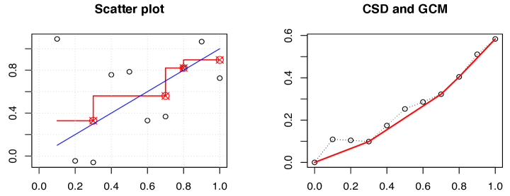
Figure 2: The left panel shows the scatter plot with the fitted function $\hat{f}_{n}$ (in red) and the true $f$ (in blue) while the right panel shows the CSD (dashed) along with its GCM (in red). Here $n=10$, $f(x)=x$ and $\varepsilon\sim N_{n}(0,\sigma^{2}I_{n})$ with $\sigma=0.5$.

Fix $0<t<1$ and suppose that $f$ has a positive continuous derivative $f^{\prime}$ on some neighborhood of $t$. The following gives the asymptotic distribution of $\hat{f}_{n}(t)$, properly normalized:

$$\Delta_{n}:=n^{1/3}\{\hat{f}_{n}(t)-f(t)\}\stackrel{{\scriptstyle d}}{{\to}}\kappa\mathbb{C},$$ (44)

where $\mathbb{C}:=\arg\min_{h\in\mathbb{R}}\{\mathbb{W}(h)+h^{2}\}$ has Chernoff’s distribution (here $\mathbb{W}(\cdot)$ is a two-sided Brownian motion starting from 0) and $\kappa:=[4\sigma^{2}f^{\prime}(t)]^{1/3}$; see e.g., [24, 142, 54, 55]. In Section A.10 we give an outline of a proof of (44). The first result of this type was derived in [115] for the Grenander estimator — the maximum likelihood estimator of a nonincreasing density in $[0,\infty)$ (see [53]). Note that the Chernoff’s random variable $\mathbb{C}$ is pivotal and its quantiles are known; see e.g., [36, 66].

4.1.1 Other asymptotic regimes.

Observe that the assumption $f^{\prime}(t)\neq 0$ is crucial in deriving the limiting distribution in (44). One may ask, what if $f^{\prime}(t)=0$? Or even simply, what if $f$ is a constant function on [0,1]? In the latter case, we can easily show that, for $t\in(0,1)$,

$$\sqrt{n}\{\hat{f}_{n}(t)-f(t)\}\stackrel{{\scriptstyle d}}{{\to}}\sigma[\tilde{\mathbb{B}}]^{\prime}(t),$$

where $\mathbb{B}$ is the standard Brownian motion on $[0,1]$. The above holds because of the following observations. First note that $\sqrt{n}\{\hat{f}_{n}(t)-f(t)\}$ is the left-hand slope of the GCM of $\sqrt{n}(F_{n}-F)$ at $t$ (as $F$ is now linear). As $\sqrt{n}(F_{n}-F)$ converges in distribution to the process $\sigma\mathbb{B}$ on $D[0,1]$, we have

$$\sqrt{n}\{\hat{f}_{n}(t)-f(t)\}=\sqrt{n}[\widetilde{F_{n}-F}]^{\prime}(t)\stackrel{{\scriptstyle d}}{{\to}}\sigma[\tilde{\mathbb{B}}]^{\prime}(t).$$

The above heuristic can be justified rigorously; see e.g., [59, Section 3.2]. In the related (nonincreasing) density estimation problem, [55, 25] showed that if $f(t)$ lies on a flat stretch of the underlying function $f$ then the LSE (which is also the nonparametric maximum likelihood estimator, usually known as the Grenander estimator) converges to a non-degenerate limit at rate $n^{-1/2}$, and they characterized the limiting distribution.

If one assumes that $f^{(j)}(t)=0$, for $j=1,\ldots,p-1$, and $f^{(p)}(t)\neq 0$ (for $p\geq 1$), where $f^{(j)}$ denotes the $j$’th derivative of $f$, then one can derive the limiting distribution of $\hat{f}_{n}(t)$, which now converges at the rate $n^{-p/(2p+1)}$; see e.g., [142, 88]. Note that all the above scenarios illustrate that the rate of convergence of the isotonic LSE $\hat{f}_{n}(t)$ crucially depends on the the behavior of $f$ around $t$; this demonstrates the adaptive behavior of the isotonic LSE from a pointwise asymptotics standpoint.

4.2 Constructing asymptotically valid pointwise confidence intervals

Although (44) gives the asymptotic distribution of the isotonic LSE at the point $t$, it is not immediately clear how it can be used to construct a confidence interval for $f(t)$ — the limiting distribution involves the nuisance parameter $f^{\prime}(t)$ that needs to be estimated. A naive approach would suggest plugging in an estimator of $f^{\prime}(t)$ in the limiting distribution in (44) to construct an approximate confidence interval. However, as $\hat{f}_{n}$ is a piecewise constant function, $\hat{f}_{n}^{\prime}$ is either 0 or undefined and cannot be used to estimate $f^{\prime}(t)$ consistently. This motivates the use of bootstrap and likelihood ratio based methods to construct confidence intervals for $f(t)$. In the following we just assume that $\varepsilon_{1},\ldots,\varepsilon_{n}$ i.i.d. mean zero errors with finite variance.

4.2.1 Bootstrap based inference.

Let us revisit (44) and consider the problem of bootstrapping $\hat{f}_{n}$ to estimate the distribution of $\Delta_{n}\sim H_{n}$ (say). Suppose that $\hat{H}_{n}$ is an approximation of $H_{n}$ (which will be obtained from bootstrap in this subsection) that can be computed. Then, an approximate $1-\alpha$ ($0<\alpha<1$) confidence interval for $f(t)$ would be

$$[\hat{f}_{n}(t)-\hat{q}_{1-\alpha/2}n^{-1/3},\hat{f}_{n}(t)-\hat{q}_{\alpha/2}n^{-1/3}],$$

where $\hat{q}_{\alpha}$ denotes the $\alpha$’th quantile of $\hat{H}_{n}$.

In a regression setup there are two main bootstrapping techniques: ‘bootstrapping pairs’ and ‘bootstrapping residuals’. Bootstrapping pairs refers to drawing with replacement samples from the data $\{(x_{i},y_{i}):i=1,\ldots,n\}$; it is more natural when we have i.i.d. bivariate data from a joint distribution. The residual bootstrap procedure fixes the design points $x_{i}$’s and draws

$$y_{i}^{*}:=\check{f}_{n}(x_{i})+\varepsilon^{*}_{i},\quad\;\;i=1,\ldots,n$$

(the ^∗ indicates a data point in the bootstrap sample) where $\check{f}_{n}$ is a natural estimator of $f$ in the model, and $\varepsilon^{*}_{i}$’s are i.i.d. (conditional on the data) having the distribution of the (centered) residuals $\{y_{i}-\check{f}_{n}(x_{i}):i=1,\ldots,n\}$. Let $\hat{f}_{n}^{*}$ denote the isotonic LSE computed from the bootstrap sample. The bootstrap counterpart of $\Delta_{n}$ (cf. (44)) is

$$\Delta^{*}_{n}:=n^{1/3}\{\hat{f}_{n}^{*}(t)-\check{f}_{n}(t)\}.$$

We now approximate $H_{n}$ by $\hat{H}_{n}$, the conditional distribution of $\Delta^{*}_{n}$, given the data. Note that a natural candidate for $\check{f}_{n}$ in isotonic regression is the LSE $\hat{f}_{n}$.

Will this bootstrap approximation (by $\hat{H}_{n}$) work? This brings us to the notion of consistency of the bootstrap. Let $d$ denote the Levy metric or any other metric metrizing weak convergence of distributions. We say that $\hat{H}_{n}$ is weakly consistent if $d(H_{n},\hat{H}_{n})\stackrel{{\scriptstyle}}{{\rightarrow}}0$ in probability. If the convergence holds with probability 1, then we say that the bootstrap is strongly consistent. If $H_{n}$ has a weak limit $H$, then consistency requires $\hat{H}_{n}$ to converge weakly to $H$, in probability; and if $H$ is continuous, consistency requires $\sup_{x\in\mathbb{R}}|\hat{H}_{n}(x)-H(x)|\stackrel{{\scriptstyle}}{{\rightarrow}}0$ in probability.

It is well-known that both the above bootstrap schemes — bootstrapping pairs and bootstrapping residuals with $\check{f}_{n}=\hat{f}_{n}$ — yield inconsistent estimators of $H_{n}$; see [1, 122, 82, 125, 56]. Intuitively, the inconsistency of the residual bootstrap procedure can be attributed to the lack of smoothness of $\hat{f}_{n}$. Indeed a version of the residual bootstrap where one considers $\check{f}_{n}$ as a smoothed version of $\hat{f}_{n}$ (that can approximate the nuisance parameter $f^{\prime}(t)$ consistently) can be shown to be consistent; see e.g., [125]. Specifically, suppose that $\check{f}_{n}$ is a sequence of estimators such that

$$\lim_{n\rightarrow\infty}\sup_{x\in I}\big{|}\check{f}_{n}(x)-f(x)\big{|}=0,$$ (45)

almost surely, where $I\subset[0,1]$ is an open neighborhood of $t$, and

$$\lim_{n\rightarrow\infty}\sup_{h\in K}n^{1/3}\big{|}\check{f}_{n}(t+n^{-1/3}h)-\check{f}_{n}(t)-f^{\prime}(t)n^{-1/3}h\big{|}=0$$ (46)

almost surely for any compact set $K\subset\mathbb{R}$. It can be shown, using arguments similar to those in the proof of [125, Theorem 2.1], that if (45) and (46) hold then, conditional on the data, the bootstrap estimator $\Delta_{n}^{*}$ converges in distribution to $\kappa\mathbb{C}$, as defined in (44), almost surely. Thus, this bootstrap scheme is strongly consistent.

A natural question that arises now is: Can we construct a smooth $\check{f}_{n}$ such that (45) and (46) hold w.p. 1? We briefly describe such a smoothed bootstrap scheme. Let $k(\cdot)$ be a differentiable symmetric density (kernel) with compact support (e.g., $k(x)\propto(1-x^{2})^{2}{\mathbf{1}}_{[-1,1]}(x)$) and let $K(x):=\int_{-\infty}^{x}k(s)\,ds$ be the corresponding distribution function. Let $h$ be a smoothing parameter. Note that $h$ may depend on the sample size $n$ but, for notational convenience, we write $h$ instead of $h_{n}$. Let $k_{h}(x):=k(x/h)/h\mbox{ and }K_{h}(x):=K(x/h).$ Then the smoothed isotonic LSE of $f$ is defined as (cf. [64])

$$\check{f}_{n}(x)\equiv\check{f}_{n,h}(x):=\int K_{h}(x-s)\,d\hat{f}_{n}(s),\quad x\in[0,1].$$

It can be easily seen that $\check{f}_{n}$ is a nondecreasing function (if $t_{2}>t_{1}$, then $K_{h}(t_{2}-s)\geq K_{h}(t_{1}-s)$ for all $s$). Observe that $\check{f}_{n}$ is a smoothed version of the step function $\hat{f}_{n}$. In [125] it is shown that the obtained bootstrap procedure is strongly consistent, i.e., $\Delta^{*}_{n}=n^{1/3}\{\hat{f}_{n}^{*}(t)-\check{f}_{n}(t)\}$ converges weakly to $\kappa\mathbb{C}$, conditional on the data, almost surely.

It is natural to conjecture that a (suitably) smoothed bootstrap procedure would also yield (asymptotically) valid pointwise confidence intervals for other shape-restricted regression functions (e.g., convex regression). Moreover, it can be expected that the naive ‘with replacement’ bootstrap and the residual bootstrap using the LSE would lead to inconsistent procedures. However, as far as we are aware, there is no work that rigorously proves these claims.

4.2.2 Likelihood ratio based inference.

Banerjee and Wellner [15] proposed a novel method for constructing pointwise confidence intervals for a monotone function (e.g., $f$) that avoids the need to estimate nuisance parameters; also see [13, 60]. Specifically, the strategy is to consider the testing problem $H_{0}:f(t)=\phi_{0}$ versus $H_{1}:f(t)\neq\phi_{0}$, where $\phi_{0}\in\mathbb{R}$ is a known constant, using the likelihood ratio statistic (LRS), constructed under the assumption of i.i.d. Gaussian errors. If one could find the limiting distribution of the LRS under the null hypothesis and show that the limit is pivotal (as is the case in parametric models where the limiting distribution turns out to be $\chi^{2}$) then that would provide a convenient way to construct a confidence interval for $f(t)$ via the method of inversion: an asymptotic level $1-\alpha$ confidence set would be given by the set of all $\phi_{0}$’s for which the null hypothesis $H_{0}:f(t)=\phi_{0}$ is accepted.

To study the form of the LRS, we first need to understand the constrained isotonic LSE. Consider the setup introduced in the beginning of Subsection 4.1 and suppose that $l:=\lfloor nt\rfloor$, so that $l/n\leq t<(l+1)/n$. Under $H_{0}:f(t)=\phi_{0}$, the constrained isotonic LSE $\hat{f}_{n}^{0}$ is given by

$$\big{\{}\hat{f}_{n}^{0}(i/n):i=1,\ldots,n\big{\}}:=\operatorname*{arg\,min}_{\theta\in\mathbb{R}^{n}:\theta_{1}\leq\cdots\leq\theta_{l}\leq\phi_{0}\leq\theta_{l+1}\leq\cdots\leq\theta_{n}}\sum_{i=1}^{n}(Y_{i}-\theta_{i})^{2}.$$

Note that both functions $\hat{f}_{n}$ and $\hat{f}_{n}^{0}$ are identified only at the design points. By convention, we extend them as left-continuous piecewise constant functions defined on the entire interval (0, 1]. The hypothesis test is based on the following LRS:

$$L_{n}:=\sum_{i=1}^{n}\big{(}Y_{i}-\hat{f}_{n}^{0}(i/n)\big{)}^{2}-\sum_{i=1}^{n}\big{(}Y_{i}-\hat{f}_{n}(i/n)\big{)}^{2}.$$

As shown in [13, 14] (in the setting of random design, which can be easily generalized to cover the uniform grid design; see [7]), if $f(t)=\phi_{0}$ and $f^{\prime}(t)\neq 0$, then

$$L_{n}\stackrel{{\scriptstyle d}}{{\to}}\sigma^{2}L,$$

where $L$ is a nonnegative random variable expressible as a functional of two-sided Brownian motion plus quadratic drift $\{\mathbb{W}(h)+h^{2}:h\in\mathbb{R}\}$, and $\sigma^{2}$ is the common variance of the errors. An important feature of this limiting distribution is that it is pivotal — free of the parameters of the problem. This readily yields confidence sets for $f(t)$ (obtained by the method of inversion) that do not need estimation of the nuisance parameter $f^{\prime}(t)$ — a challenging quantity to estimate in practice. However, an estimate of $\sigma^{2}$ is required, which can be easily obtained: The natural estimator $\|Y-\hat{\theta}\|^{2}/n$ of $\sigma^{2}$ is asymptotically normal with mean $\sigma^{2}$ and variance $2\sigma^{4}/n$ (see [102, Proposition 3]). This methodology has been applied successfully in several monotone function estimation problems; see e.g., [15, 13, 60]. The method, and extensions thereof, also applies to both short- and long-range dependence regimes for the errors; see [7]. Also see [16, 7] for illustrations and examples of the superior performance of the LR based method over plug-in methods for constructing confidence intervals for $f(t)$, especially when the estimation of the derivative $f^{\prime}(t)$ is difficult.

Not much is known about the (asymptotic) distribution of the LRS beyond monotone function estimation problems. However, in the recent papers [40, 41] the authors study the LRS for testing the location of the mode of a log-concave density $f$ using the unconstrained/constrained maximum likelihood estimator of a log-concave density (also see [11]) and show that, under the null hypothesis which fixes the value of the mode of $f$ (and assumes strict curvature of $-\log f$ at the mode), the LRS is asymptotically pivotal.

4.3 Pointwise limit theory of the LSE in convex regression

We assume that we have data from (1) where $f:[0,1]\to\mathbb{R}$ is now assumed to be convex (see Example 1.3). In this section we study the pointwise asymptotic theory for the convex LSE. For simplicity, as before, we consider equi-spaced design points. Let us first describe the characterization of the convex LSE that will drive the asymptotic analysis. Given the convex LSE $\hat{\theta}$, let $\hat{\Theta}=(\hat{\Theta}_{1},\ldots,\hat{\Theta}_{n})$ denote the vector of its cumulative sums (divided by $n$), i.e., $\hat{\Theta}_{i}:=n^{-1}\sum_{j=1}^{i}\hat{\theta}_{j}$, for $i=1,\ldots,n,$ and recall $F_{n}$, as defined in (43). Then, $\hat{\theta}$ has the following characterization: $\hat{\theta}$ is the unique vector such that $\hat{\Theta}_{n}=F_{n}(1)$ and

$$\sum_{i=1}^{j-1}\hat{\Theta}_{i}\begin{cases}\geq\sum_{i=1}^{j-1}F_{n}(i/n)&\mbox{for }\;j=2,\ldots,n,\\ =\sum_{i=1}^{j-1}F_{n}(i/n)&\mbox{if $\hat{\theta}$ has a kink at $j/n$ or $j=n$;}\end{cases}$$ (47)

this follows from the characterization of projection on the closed convex set $\mathcal{K}$ (as defined in (6)); see [62, Lemma 2.6] for a complete proof. We define the convex LSE $\hat{f}_{n}:[1/n,1]\to\mathbb{R}$ of $f$ as the piecewise linear interpolation of the points $\{(i/n,\hat{\theta}_{i}):i=1,\ldots,n\}$.

Fix $t\in(0,1)$ and consider the estimation of $f(t)$ using the convex LSE $\hat{f}_{n}(t)$ under the assumption that $f^{\prime\prime}$ is continuous and nonzero in a neighborhood of $t$. If the errors are i.i.d. sub-Gaussian with mean zero and $f^{\prime\prime}(t)\neq 0$, the rate of convergence of $\hat{f}_{n}(t)$ is known to be $n^{-2/5}$ (see [94]). The pointwise asymptotic distribution of the convex LSE (properly normalized) is derived in [62]. In Groeneboom et al. [62] the authors show that

$$\Delta_{n}:=n^{2/5}\{\hat{f}_{n}(t)-f(t)\}\stackrel{{\scriptstyle d}}{{\to}}\mathbb{H}^{\prime\prime}(0),$$ (48)

where $\mathbb{H}$ is the “invelope” of integrated Brownian motion with quartic drift ($+h^{4}$), and $\mathbb{H}^{\prime\prime}(0)$ is the second derivative of $\mathbb{H}$ at 0 (which exists w.p. 1). The invelope is a cubic spline lying above and touching integrated Brownian motion $+h^{4}$; compare this with the “envelope” of Brownian motion with a parabolic drift ($+h^{2}$) that appears when analyzing the isotonic LSE (see Section A.10). Although a rigorous proof of the above weak convergence is long and delicate (see [62, Theorem 6.3]), the main intuition for such a limit can be gotten from looking at the characterization given in (47). We describe some of the main ideas below. The first step is to show that the characterization in (47) can be ‘localized’ in an appropriate sense. Then we show that the right side of the inequality in (47), appropriately localized and normalized, converges to a limiting process involving integrated Brownian motion $+h^{4}$. Then, a continuous mapping-like result, where we look at the limiting version of the localized (47), yields the convergence of $\Delta_{n}$. A slightly more detailed sketch of the main steps is provided in Section A.11.

Remark 4.1 (Multiscale inference in shape-restricted problems).

The pointwise asymptotic theory for isotonic and convex regression is developed under suitable smoothness assumptions on $f$, e.g., (44) needs $f^{\prime}(t)\neq 0$ whereas the weak convergence of (48) assumes $f^{\prime\prime}(t)\neq 0$. In [42], utilizing suitable multiscale tests, the author constructs confidence bands for $f$ that are locally adaptive in a certain sense (to the underlying smoothness in $f$) and have guaranteed coverage, assuming that $f$ is isotonic or convex. These confidence bands are computationally feasible and are also shown to be asymptotically sharp optimal in an appropriate sense. Also see the recent paper [144] for another method of constructing finite-sample locally adaptive confidence bands in isotonic regression.

5 Computation of the LSE

In this section we discuss the computation of the LSE $\hat{\theta}$ in nonparametric shape-restricted regression problems. Note that in most cases (see e.g., Examples 1.1–1.5) the LSE $\hat{\theta}$ is the projection of $Y$ onto $\mathcal{C}$, a (finite union of) closed convex set(s) in $\mathbb{R}^{n}$. If $\mathcal{C}$ is a polyhedral convex set, then the computation of $\hat{\theta}$ involves solving a quadratic program with a bunch of linear constraints. Many off-the-shelf solvers — e.g., CPLEX, MOSEK, Gurobi — can solve these quadratic programs easily even for moderately large sample sizes (e.g., $n\approx 10^{5}$). In the following we consider the main examples in the Introduction and discuss some problem specific algorithms that are computationally more efficient.

Isotonic and unimodal regression. For the monotone regression problem [17] presented a graphical interpretation of the isotonic LSE (defined in (11)) in terms of the GCM of the CSD; see Section 4.1. The method of successive approximation to the GCM can be described algebraically as the pool-adjacent-violators algorithm (PAVA); see e.g., [118, p. 9-10]. Roughly speaking, PAVA works as follows. We start with $y_{1}$ on the left. We move to the right until we encounter the first violation $y_{i}>y_{i+1}$. Then we replace this pair by their average, and back-average to the left as needed, to get monotonicity. We continue this process to the right, until finally we reach $y_{n}$. If skillfully implemented, PAVA has a computational complexity of $O(n)$; see [131] for a comparison of various algorithms to solve isotonic regression in $\ell_{p}$-metrics, for $p\geq 1$. The isoreg command in the stats package in the R programming language implements the isotonic LSE. Further, see [130] for an efficient (requiring only $O(n)$ time) computation of the unimodal LSE (Example 1.4).

Order preserving regression on a partially ordered set. Given a partial order $\precsim$ on the design points $x_{i}$’s we can compute the LSE $\hat{\theta}$ of the isotonic (order preserving) $\theta^{*}$ by solving (7). Here $\mathcal{C}$, the space where $Y$ is projected onto to obtain $\hat{\theta}$, is a closed convex cone and can be represented as

$$\mathcal{C}:=\{(\theta_{1},\ldots,\theta_{n})\in\mathbb{R}^{d}:\theta_{i}\leq\theta_{j}\mbox{ if }x_{i}\precsim x_{j},\mbox{ for some }i\neq j\}.$$

Thus, the computation of $\hat{\theta}$ involves solving a quadratic program with $O(n^{2})$ linear constraints (although for some special situations, like isotonic regression in $d=1$, $\mathcal{C}$ can be represented by $O(n)$ linear constraints). The computation of the order preserving LSE on a partially ordered set (Example 1.2) has received quite a bit of attention recently; see e.g., [87, 132] and the references therein. In particular, https://github.com/sachdevasushant/Isotonic gives an implementation of the isotonic LSE using interior point methods. The special case of the matrix isotonic LSE defined in (26) can be computed efficiently by an iterative algorithm (see e.g., [51] and [118, Chapter 1]).

Once we obtain $\hat{\theta}=(\hat{\theta}_{1},\ldots,\hat{\theta}_{n})$ we can then easily construct an estimate $\hat{f}_{n}$ of the order preserving $f$ at any $x$ (not necessarily a design point) by taking a maximum over a selected number of coordinates of $\hat{\theta}$: We can define $\hat{f}_{n}$ as

$$\hat{f}_{n}(x):=\sup_{j:x_{j}\precsim\;x}\hat{\theta}_{j},\quad\mbox{for }x\in\mathbb{R}^{d},$$

where we take the convention that $\sup(\emptyset)=-\infty$. Note that $\hat{f}_{n}$ is indeed order preserving — for $u,v$ with $u\precsim v$ we have $\hat{f}_{n}(u)=\sup_{j:x_{j}\precsim\;u}\hat{\theta}_{j}\leq\sup_{j:x_{j}\precsim\;v}\hat{\theta}_{j}=\hat{f}_{n}(v),$ as in the right side the supremum is taken over a bigger set.

Convex regression. Algorithms for the computation of the convex LSE (Example 1.3) when $d=1$ can be found in [45], [48], [63] and the references therein. When $d>1$, the problem is substantially harder: Due to the lack of a natural ordering of points in $\mathbb{R}^{d}$ (for $d>1$), the constraint set $\mathcal{C}$ is not easy to express (cf. (6)). In fact, in this case $\mathcal{C}$ can be expressed as the projection of the higher-dimensional polyhedron

$$\left\{(\xi,\theta)\in\mathbb{R}^{dn+n}:\xi=[\xi_{1}^{\top},\ldots,\xi_{n}^{\top}]^{\top},\theta_{j}+\xi_{j}^{\top}(x_{i}-x_{j})\leq\theta_{i},\forall\;i,j=1,\dots,n\right\}$$

onto the space of $\theta$; see [34]. The above characterization can be seen as a consequence of the subgradient inequality for convex functions; see [119, Theorem 25.1, p. 242]. Thus the computation of the convex LSE $\hat{\theta}$ involves solving a quadratic program with $n(d+1)$ variables and $n(n-1)$ linear constraints; see [121] for the characterization, computation and consistency of the convex LSE where off-the-shelf interior point solvers (e.g., cvx, MOSEK, etc.) were used to compute $\hat{\theta}$. However, these off-the-shelf solvers do not scale well and become prohibitively expensive for $n\geq 300$ mainly due to the presence of $O(n^{2})$ linear constraints. In [101], exploiting problem specific structure, the authors propose a scalable algorithmic framework based on the augmented Lagrangian method to compute the convex LSE $\hat{\theta}$. This iterative algorithm can compute the LSE with $n\sim 5000$ and $d\sim 10$ within moderate accuracy (i.e., 4 significant digits) in around 30 minutes in a laptop.

Shape constrained additive models. The computation of the additive shape-restricted (Example 1.5) LSE is discussed in [106, 35]. As this reduces to solving a quadratic program with $O(n)$ linear constraints, off-the-shelf solvers can be effectively used for computing the LSE. The shape-restricted LSE can also be computed efficiently by the back-fitting algorithm ([22]) — a simple iterative procedure used to fit a generalized additive model — which involves fitting one function at a time (out of the $d$ many univariate nonparametric functions).

Shape-restricted single index model. Let us now look at Example 1.6. Here interest focuses on estimating the nonparametric (shape-restricted) function $m$ and the finite-dimensional parameter $\beta^{*}$. Although single index models are well-studied in the statistical literature (see e.g., [114], [89], [37] and the references therein), estimation and inference in shape-restricted single index models are not very well-developed, despite their numerous applications. The LSE in the monotone single index model is defined as

$$(\hat{m},\hat{\beta}):=\operatorname*{arg\,min}_{\psi,\beta}\sum_{i=1}^{n}(y_{i}-\psi(x_{i}^{\top}\beta))^{2},$$ (49)

where the minimization is over all nondecreasing functions $\psi:\mathbb{R}\to\mathbb{R}$ and over $\beta\in\mathbb{R}^{d}$ (with $\|\beta\|=1$, for identifiability). As the above LSE solves a non-convex problem, its computation is non-trivial. A version of the following alternating minimization scheme is typically applied to compute the LSE. For a fixed $\beta$, the sum-of-squared errors can be easily minimized over all nondecreasing functions (as this reduces to the problem to univariate isotonic regression). However, the minimization of the profiled least squares criterion (over $\beta$), for a fixed $\psi$, is non-smooth and non-convex; see [78, 57] and the references therein for some strategies to find $\hat{\beta}$. A similar strategy is employed in computing the maximum likelihood estimate in the related problem of current status regression; see e.g., [57]. Also see [84] and the R package simest for the related computation in a convex single index model.

6 Some open problems

In this section we state and motivate a few open research problems and some possible future directions.

Beyond i.i.d. Gaussian errors. We have mentioned in Section 2 that risk bounds for isotonic regression do not assume that the errors $\varepsilon_{1},\dots,\varepsilon_{n}$ are Gaussian. Indeed, the worst case risk bound (12) as well as the adaptive risk bound in Theorem 2.1 work under no distributional assumptions on the errors (it is only assumed that the errors are i.i.d. with mean zero and finite variance $\sigma^{2}$; even the i.i.d. assumption can be relaxed considerably; see [146]). However the risk bounds for other shape-restricted regression problems (including convex regression, isotonic regression on partially ordered sets such as multivariate isotonic regression, unimodal regression, etc.) assume Gaussian (or sub-Gaussian) errors. Based on the results for the univariate isotonic LSE, we believe that the assumption of Gaussianity should not really be necessary for these other problems as well. However the existing proof techniques for these risk bounds strongly rely on the assumption of sub-Gaussianity. It will be very interesting to prove risk bounds in these problems without Gaussianity. We believe that new techniques will need to be developed for this.

Beyond $\ell_{2}$-loss. Most of the risk results available in the shape constrained literature apply only to the $\ell_{2}$-loss. A notable exception is the case of isotonic regression where risk bounds are available under the $\ell_{p}$-loss for every $p\geq 1$ (as already described in Subsection 2.2.1). It will be interesting to develop risk results for $\ell_{p}$-losses in problems such as convex regression and multivariate shape-restricted regression. The results for isotonic regression (see Theorem 2.2 and the following discussion) indicate that adaptation risk bounds for LSEs have a different relationship with oracle risk bounds for $p\neq 2$. For example, for $p<2$, the isotonic LSE is suboptimal only by a constant factor in comparison to the oracle while for $p>2$, the isotonic LSE is significantly suboptimal. We believe that it is quite non-trivial to study risk of the LSEs under $\ell_{p}$-loss functions for $p\neq 2$. The existing abstract theory for studying LSEs seems to give risk results only under the $\ell_{2}$-loss function.

Minimax Results. The risk of a LSE $R(\hat{\theta},\theta^{*})$ in a shape-restricted regression problem usually varies quite significantly as $\theta^{*}$ varies over the parameter space. For example, in isotonic regression, the risk behaves as $n^{-2/3}$ when $V(\theta^{*})$ is bounded and as $(k/n)\log(n/k)$ when $\theta^{*}$ is piecewise constant having $k$ constant pieces. Minimax lower bounds over these parameter classes allow the assessment of optimality of the LSE compared to other estimators. We mentioned in Remark 2.3 that the isotonic LSE is minimax optimal over $\{\theta\in\mathcal{I}:\theta_{n}-\theta_{1}\leq V\}$ for a wide range of values of $V$. In an interesting recent paper [50], the authors characterized the minimax risk over the class of all monotone vectors with at most $k$ constant pieces. Their results imply that the risk $(k/n)(\log(n/k))$ achieved by the isotonic LSE over this class is only suboptimal by a factor of $(\log n)/(\log\log n)$ in comparison to the minimax risk. Minimax lower bounds exist for other shape-restricted regression problems (see e.g., [68, 28, 19, 69, 31]) which suggest that the LSE is nearly minimax optimal but some of these results are not as tight as the corresponding results for univariate isotonic regression. It will be interesting to develop tight minimax results for other shape-restricted regression problems which will allow a precise evaluation of the minimaxity properties of the LSEs.

Estimation of other shape constrained regression functions. In the recent years there has been quite a bit of interest in studying different shape-restricted regression functions, beyond $d=1$. We have already seen a few such examples in this paper (e.g., Examples 1.2, 1.3 and 1.5). What are other useful shape-restrictions in multi-dimension? In the following we mention a few such shape constraints (that have many real applications): (i) unordered weak majorization, (ii) quasiconvexity, and (iii) supermodularity.

Unordered weak majorization. In Example 1.2 we discussed the problem of estimating an order preserving regression function (with respect to a partial order). Robertson et al. [118, Chapter 1] gives a nice overview of the properties of the LSE in this problem. As an example we introduced a generalization of monotonicity beyond $d=1$, namely, coordinate-wise monotonicity. In the following we introduce and characterize another related (and slightly stronger) notion of monotonicity in multi-dimensions that is closely tied to the concept of majorization and Schur-convexity (see e.g., [99]). We define the unordered weak majorization partial order $\precsim$ as

$$(u_{1},\ldots,u_{d})\precsim(v_{1},\ldots,v_{d})\;\;\mbox{if and only if}\;\;\sum_{k=1}^{i}u_{k}\leq\sum_{k=1}^{i}v_{k}\;\;\mbox{for }i=1,2,\ldots,d.$$

The following result characterizes all functions that preserve the ordering $\precsim$.

Theorem 6.1.

Let $f:\mathbb{R}^{d}\to\mathbb{R}$ be a continuously differentiable function. Then $f$ preserves the partial order $\precsim$ if and only if for any $z\in\mathbb{R}^{d}$,

$$f_{(1)}(z)\geq f_{(2)}(z)\geq\ldots\geq f_{(d)}(z)\geq 0,$$ (50)

where $f_{(i)}$ denotes the partial derivate of $f$ with respect to the $i$’th coordinate.

The above result shows that in a regression setup if $f$ can be assumed to obey (50), i.e., the influence of the predictor variables is ordered, LS estimation under the unordered weak majorization partial order can be used to estimate $f$. Constraints like (50) appear quite often in econometrics; see e.g., [145] and the references therein.

Quasiconvexity. A function $f:\mathbb{R}^{d}\to\mathbb{R}$ is quasiconvex if and only if its sub-level sets $S_{\alpha}(f)=\{u\in\mathbb{R}^{d}:f(u)\leq\alpha\}$ are convex for every $\alpha\in\mathbb{R}$; see [21, Section 3.4]. Alternatively, a function $f$ is quasiconvex if and only if $f(\alpha u+(1-\alpha)v)\leq\max\{f(u),f(v)\}$, for all $u,v\in\mathbb{R}^{n}$, and $\alpha\in[0,1]$ (cf. (5)). Quasiconvex functions extend the notion of unimodality to multi-dimensions and have applications in mathematical optimization and economics. The computation of $f$ using the method of least squares is likely to be a non-convex problem.

Supermodularity. A function $f:\mathbb{R}^{d}\to\mathbb{R}$ is supermodular if $f(u\vee v)+f(u\wedge v)\geq f(u)+f(v)$ for all $u,v\in\mathbb{R}^{d}$, where $u\vee v$ and $u\wedge v$ denote the component-wise maximum and minimum of $u$ and $v$, respectively, i.e., $(u_{1},\ldots,u_{d})\vee(v_{1},\ldots,v_{d}):=(\max\{u_{1},v_{1}\},\ldots,\max\{u_{d},v_{d}\})$ and $(u_{1},\ldots,u_{d})\wedge(v_{1},\ldots,v_{d}):=(\min\{u_{1},v_{1}\},$ $\ldots,\min\{u_{d},v_{d}\})$. The concept of supermodularity is used in the social sciences (economics and game theory). If $f$ is twice continuously differentiable, then supermodularity is equivalent to the condition $\frac{\partial^{2}f(u)}{\partial u_{i}\,\partial u_{j}}\geq 0$ for all $i\neq j$; see e.g., [128].

In all the above problems, computation of the LSE, its theoretical properties (consistency, rates of convergence, etc.) are unknown.

Connection to nonnegative least squares. In many shape-restricted regression problems the LSE $\hat{\theta}$ is defined as the projection of $Y$ onto a closed convex polyhedral cone $\mathcal{C}$; see Examples 1.1–1.3 and 1.5. As every closed convex polyhedral cone $\mathcal{C}$ in $\mathbb{R}^{n}$ can be represented in terms of its generators (i.e., there exists a finite subset of $\mathcal{C}$, whose elements are referred to as generators of $\mathcal{C}$, such that every vector $\theta\in\mathcal{C}$ is a nonnegative linear combination of the generators; see, for example, [120, Corollary 7.1a]), $\hat{\theta}$ can be thought of as solving a nonnegative least squares problem. Moreover, in the examples mentioned above, $\mathcal{C}$ is generated by at least $O(n)$ vectors (which form the design matrix) that are highly correlated; see e.g., [103] for the exact form of the generators of some of the examples discussed. In fact, for isotonic and convex regression in $d=1$ there are exactly $n+1$ and $n+2$ generators, respectively. However, for their higher dimensional analogues (i.e., $d>1$) it is not clear what the generators are. We think this is an open problem. More generally, one can ask how does one construct the design matrix (or the generators) corresponding to any closed convex polyhedral cone expressed in terms of linear inequalities, e.g., $\mathcal{C}:=\{\theta\in\mathbb{R}^{n}:A\theta\leq 0\}$ where $A$ is an $m\times n$ matrix ($m$ being the number of linear constraints) and the ‘$\leq$’ is interpreted coordinate-wise.

As the number of generators (or the columns of the design matrix) is increasing with $n$, we are essentially solving a ‘high-dimensional’ nonnegative least squares problem; see e.g., [129]. A general open question is: Can a theory be developed on the estimation accuracy of the LSE $\hat{\theta}$ based solely on the properties of the design matrix? It may be noted here that the generators can be highly correlated.

Boundary behavior of shape-restricted LSEs. It is well known that the isotonic LSE is inconsistent at the boundary of the covariate domain, i.e., $\hat{f}_{n}(0+)$ does not consistently estimate $f(0+)$ (see e.g., [141, 85, 10] for detailed discussions on the properties of the LSE for a nonincreasing density near 0). Intuitively, this inconsistency is because there are very few ‘constraints’ near the boundary (of the covariates). This phenomenon is expected to persist for other shape constrained LSEs, especially in multi-dimensional problems. However not much is known about the boundary behavior of these LSEs. Even in one-dimensional convex regression, as far as we are aware, whether $\hat{f}_{n}(0+)$ is a $O_{p}(1)$ random variable is not known; see [52] for some results on $\hat{f}_{n}(0+)$ and its derivative (also see [8]). This has motivated the study of bounded/penalized shape-restricted LSEs; see e.g., [34, 143, 84].

Shape-restricted single index models. Although several smoothing based methods have been proposed and investigated in single index models (see e.g., [108, 57] and the references therein) to obtain $\sqrt{n}$-consistent and efficient estimators of $\beta^{*}$ (see [110] for a brief overview of the notion of semiparametric efficiency), not much is known for just shape-restricted single index models. Durot et al. [9] studied the LSE in a monotone single index model (see (49)) and showed the $n^{1/3}$-consistency of the LSEs of $m$ and $\beta^{*}$; also see [108] and [57]. However many open questions remain. The limiting distribution of the LSE $\hat{\beta}$ of $\beta^{*}$ is unknown; in fact, it is not known whether $\hat{\beta}$ is $\sqrt{n}$-consistent.

In a convex single index model (i.e., $m$ is convex), [84] shows that the Lipschitz constrained convex LSE (where we minimize the least squares criterion over the class of all $L$-Lipschitz convex functions, for $L$ fixed) yields a semiparametrically efficient estimator of the index parameter $\beta^{*}$. However, the behavior of the convex LSE (without the Lipschitz assumption) is unknown.

As mentioned above, the computation of the shape-restricted LSEs is non-trivial. Usually an alternating minimization scheme is used to compute the LSEs. However, no convergence guarantees (to a local optimum) exist for such an alternating minimization procedure.

Appendix A Proofs

This section contains proofs of some of the results from the main paper.

A.1 Proof of Theorem 2.1

To prove the adaptive risk bound (13) for isotonic regression we shall apply inequality (39) with $Z=\varepsilon/\sigma$ which reduces the task to proving that

$$\mathbb{E}\|\Pi_{T_{\mathcal{I}}(\theta)}(Z)\|^{2}\leq 4k(\theta)\log\frac{en}{k(\theta)}\quad\mbox{for every $\theta\in\mathcal{I}$}.$$ (51)

To prove this, we obviously need to characterize the tangent cone $T_{\mathcal{I}}(\theta)$. Fix $\theta\in\mathcal{I}$ and let $k=k(\theta)$. This means that $\theta$ has $k$ constant pieces (and $k-1$ jumps). Let the lengths of the $k$ constant pieces be $n_{1},\dots,n_{k}$ (so that $n_{j}\geq 1$ and $\sum_{j=1}^{k}n_{j}=n$). It is now an easy exercise to verify (via (38)) that the tangent cone $T_{\mathcal{I}}(\theta)$ is given by

$$T_{\mathcal{I}}(\theta)=\mathcal{I}_{n_{1}}\times\dots\times\mathcal{I}_{n_{k}}$$ (52)

where $\times$ denotes Cartesian product and, for an integer $\ell\geq 1$,

$$\mathcal{I}_{\ell}:=\left\{(x_{1},\dots,x_{\ell})\in\mathbb{R}^{l}:x_{1}\leq\dots\leq x_{\ell}\right\}.$$

The equality (52) immediately implies that

$$\mathbb{E}\|\Pi_{T_{\mathcal{I}}(\theta)}(Z)\|^{2}=\sum_{j=1}^{k}\mathbb{E}\|\Pi_{{\mathcal{I}_{n_{j}}}}(Z^{(j)})\|^{2}$$ (53)

where $Z^{(j)}$ denotes the part of the vector $Z$ corresponding to the $j^{th}$ constant piece of $\theta$. The key now is to prove that

$$\mathbb{E}\|\Pi_{\mathcal{I}_{n}}(Z)\|^{2}\leq 4\left(1+\frac{1}{2}+\dots+\frac{1}{n}\right)\quad\mbox{for every $n\geq 1$}.$$ (54)

This, along with the standard fact that $\sum_{j=1}^{n}(1/j)\leq\log(en)$, implies that

$$\mathbb{E}\|\Pi_{{\mathcal{I}_{n_{j}}}}(Z^{(j)})\|^{2}\leq 4\log(en_{j}).$$

Thus, we obtain, via (53),

$$\mathbb{E}\|\Pi_{T_{\mathcal{I}}(\theta)}(Z)\|^{2}\leq\sum_{j=1}^{k}4\log(en_{j})\leq 4k\log\frac{en}{k}$$

where the last inequality follows from the concavity of the logarithm function. This proves (51) and consequently (13). To prove (54) let

$$U=(U_{1},\dots,U_{n}):=\Pi_{\mathcal{I}_{n}}(Z).$$

The representation (11) gives

$$U_{j}=\min_{v\geq j}\max_{u\leq j}\bar{Z}_{uv}\quad\mbox{for every $1\leq j\leq n$}$$

where $\bar{Z}_{uv}$ represents the mean of $Z_{u},\dots,Z_{v}$. It is clear from here that

$$U_{j}\leq\max_{u\leq j}\bar{Z}_{un}$$

so that

$$\mathbb{E}(U_{j})_{+}^{2}\leq\mathbb{E}\max_{u\leq j}(\bar{Z}_{un})_{+}^{2}.$$

Here $x_{+}:=\max(x,0)$ and $a_{+}^{2}:=(a_{+})^{2}$. The key now is to realize that the sequence of random variables $\bar{Z}_{1n},\dots,\bar{Z}_{jn}$ is a martingale (easy to verify) so that by Doob’s submartingale maximal inequality, we deduce that

$$\mathbb{E}(U_{j})_{+}^{2}\leq 4\mathbb{E}(\bar{Z}_{jn})_{+}^{2}.$$

By an analogous argument, we can also deduce that

$$\mathbb{E}(U_{j})_{-}^{2}\leq 4\mathbb{E}(\bar{Z}_{1j})_{-}^{2}$$

where $x_{-}:=\max(0,-x)$. Putting together, we deduce

$$\mathbb{E}\|\Pi_{\mathcal{I}_{n}}(Z)\|^{2}=\sum_{j=1}^{n}\mathbb{E}U_{j}^{2}\leq 4\sum_{j=1}^{n}\left(\mathbb{E}(\bar{Z}_{jn})_{+}^{2}+\mathbb{E}(\bar{Z}_{1j})_{-}^{2}\right).$$

Now because $Z_{1},\dots,Z_{n}$ are i.i.d. $(Z_{1},\dots,Z_{n})$ has the same distribution as $(Z_{n},\dots,Z_{1})$ so that

$$\mathbb{E}\|\Pi_{\mathcal{I}_{n}}(Z)\|^{2}\leq 4\sum_{j=1}^{n}\left(\mathbb{E}(\bar{Z}_{1,n-j+1})_{+}^{2}+\mathbb{E}(\bar{Z}_{n-j+1,n})_{-}^{2}\right)=4\sum_{j=1}^{n}\left(\mathbb{E}(\bar{Z}_{1j})_{+}^{2}+\mathbb{E}(\bar{Z}_{jn})_{-}^{2}\right).$$

Adding the above two inequalities, we obtain

$$2\mathbb{E}\|\Pi_{\mathcal{I}_{n}}(Z)\|^{2}\leq 4\sum_{j=1}^{n}\left(\mathbb{E}(\bar{Z}_{jn})^{2}+\mathbb{E}(\bar{Z}_{1j})^{2}\right)=4\sum_{j=1}^{n}\left(\frac{1}{n-j+1}+\frac{1}{j}\right)=8\sum_{j=1}^{n}\frac{1}{j}.$$

This proves (54) and completes the proof of (13). ∎

A.2 Proof of inequality (12)

The initial steps of this proof follow the same steps as in the beginning of the proof of Theorem 2.2 (the proof of Theorem 2.2 is provided in Subsection A.5). Specifically, we use inequality (60) for $p=2$ which says that

$$\mathbb{E}_{\theta^{*}}\left(\hat{\theta}_{j}-\theta^{*}_{j}\right)_{+}^{2}\leq\mathbb{E}_{\theta^{*}}\left(\left(\bar{\theta^{*}}_{j,j+m}-\theta^{*}_{j}\right)+\left(\max_{u\leq j}\bar{\varepsilon}_{u,j+m}\right)_{+}\right)^{2}.$$

for every $1\leq j\leq n$ and $0\leq m\leq n-j$. The elementary inequality $\mathbb{E}(c+X)^{2}\leq(c+\sqrt{\mathbb{E}X^{2}})^{2}$ for $c\geq 0$ applied to $c=\bar{\theta^{*}}_{j,j+m}-\theta^{*}_{j}\geq 0$ and $X:=\left(\max_{u\leq j}\bar{\varepsilon}_{u,j+m}\right)_{+}$ now gives

$$\mathbb{E}_{\theta^{*}}\left(\hat{\theta}_{j}-\theta^{*}_{j}\right)_{+}^{2}\leq\left(\bar{\theta^{*}}_{j,j+m}-\theta^{*}_{j}+\sqrt{\mathbb{E}\max_{u\leq j}\left(\bar{\varepsilon}_{u,j+m}\right)^{2}_{+}}\right)^{2}.$$

Doob’s maximal submartingale inequality applied to the expectation above results in

$$\mathbb{E}\max_{u\leq j}\left(\bar{\varepsilon}_{u,j+m}\right)^{2}_{+}\leq 4\mathbb{E}\left(\bar{\varepsilon}_{u,j+m}\right)^{2}_{+}\leq 4\left(\bar{\varepsilon}_{u,j+m}\right)^{2}=\frac{4\sigma^{2}}{m+1}.$$

We have thus proved that

$$\mathbb{E}_{\theta^{*}}\left(\hat{\theta}_{j}-\theta^{*}_{j}\right)_{+}^{2}\leq\min_{0\leq m\leq n-j}\left(\bar{\theta^{*}}_{j,j+m}-\theta^{*}_{j}+\frac{2\sigma}{\sqrt{m+1}}\right)^{2}.$$ (55)

Similarly, we can prove that

$$\mathbb{E}_{\theta^{*}}\left(\hat{\theta}_{j}-\theta^{*}_{j}\right)_{-}^{2}\leq\min_{0\leq m\leq j-1}\left(\theta^{*}_{j}-\bar{\theta^{*}}_{j-m,j}+\frac{2\sigma}{\sqrt{m+1}}\right)^{2}.$$ (56)

For each $1\leq j\leq n$, let us define

$$m_{1}(j):=\max\left\{0\leq m\leq n-j:\bar{\theta^{*}}_{j,j+m}-\theta^{*}_{j}\leq\frac{2\sigma}{\sqrt{m+1}}\right\}$$

and

$$m_{2}(j):=\max\left\{0\leq m\leq j-1:\theta^{*}_{j}-\bar{\theta^{*}}_{j-m,j}\leq\frac{2\sigma}{\sqrt{m+1}}\right\}.$$

Note that these choices of $m_{1}(j)$ and $m_{2}(j)$ are different from those made in the proof of Theorem 2.2. From (55) and (56), we obtain

$$\mathbb{E}_{\theta^{*}}\left|\hat{\theta}_{j}-\theta^{*}_{j}\right|^{2}\leq 16\sigma^{2}\left(\frac{1}{m_{1}(j)+1}+\frac{1}{m_{2}(j)+1}\right)$$

so that the risk of $\hat{\theta}$ is bounded by

$$R(\hat{\theta},\theta^{*})\leq\frac{16\sigma^{2}}{n}\left(\sum_{j=1}^{n}\frac{1}{m_{1}(j)+1}+\sum_{j=1}^{n}\frac{1}{m_{2}(j)+1}\right).$$ (57)

We shall bound $\sum_{j}(m_{1}(j)+1)^{-1}$ below. The bound for the term involving $m_{2}(j)$ will be similar.

For each $m\geq 0$, let

$$\rho(m):=\sum_{j=1}^{n}I\left\{m_{1}(j)=m\right\}~{}~{}~{}\text{ and }~{}~{}~{}l(m):=\sum_{j=1}^{n}I\left\{m_{1}(j)<m\right\}.$$

Clearly $\rho(m)=l(m+1)-l(m)$ and hence

$$\sum_{j=1}^{n}\frac{1}{m_{1}(j)+1}=\sum_{m\geq 0}\frac{\rho(m)}{m+1}=\sum_{m\geq 0}\frac{l(m+1)-l(m)}{m+1}=\sum_{m\geq 0}\frac{l(m+1)}{(m+1)(m+2)}$$ (58)

because $l(0)=0$. For $0\leq m\leq n-1$, we can write

$$l(m+1)=\sum_{j=1}^{n}I\{m_{1}(j)<m+1\}\leq\sum_{j=1}^{n-m-1}I\{m_{1}(j)<m+1\}+m+1.$$

When $1\leq j\leq n-m-1$ and $m_{1}(j)<m+1$, the definition of $m_{1}(j)$ implies that

$$\bar{\theta^{*}}_{j,j+m+1}-\theta^{*}_{j}>\frac{2\sigma}{\sqrt{m+2}}$$

so that

$$I\left\{m_{1}(j)<m+1\right\}<\sqrt{m+2}~{}\frac{\bar{\theta^{*}}_{j,j+m+1}-\theta^{*}_{j}}{2\sigma}\qquad\text{for $1\leq j\leq n-m-1$}.$$

and

$$l(m+1)\leq m+1+\frac{\sqrt{m+2}}{2\sigma}\sum_{j=1}^{n-m-1}\left(\bar{\theta^{*}}_{j,j+m+1}-\theta^{*}_{j}\right)\qquad\text{for $0\leq m\leq n-1$}.$$

We now use Lemma A.1 to bound the right hand side above in terms of $V:=V(\theta^{*})$. Indeed, Lemma A.1 (applied with $l=m+2$) gives

$$l(m+1)\leq m+1+\frac{(m+1)\sqrt{m+2}}{2\sigma}V.$$

Also, the trivial upper bound $l(m+1)\leq n$ always holds. We thus obtain

$$l(m+1)\leq\min\left(n,m+1+\frac{(m+1)\sqrt{m+2}}{2\sigma}V\right)\qquad\text{for all $m\geq 0$}.$$

This inequality, together with (58), gives

$$\sum_{j=1}^{n}\frac{1}{m_{1}(j)+1}\leq\sum_{m\geq 0}\frac{1}{(m+1)(m+2)}\min\left\{n,m+1+\frac{(m+1)\sqrt{m+2}}{2\sigma}V\right\}.$$

Now let

$$s:=\min\left(\left(\frac{\sigma n}{V}\right)^{2/3},n\right)$$

and write ($C$ below stands for a positive constant whose value may change from appearance to appearance; it does not depend on $n$, $V$ or $\sigma$)

$$\sum_{j=1}^{n}\frac{1}{m_{1}(j)+1} \leq\sum_{m\geq 0}\frac{1}{(m+1)(m+2)}\min\left\{n,m+1+\frac{(m+1)\sqrt{m+2}}{2\sigma}V\right\}$$

$$\leq\sum_{0\leq m\leq s}\frac{(m+1)+(m+1)\sqrt{m+2}(V/(2\sigma))}{(m+1)(m+2)}+n\sum_{m>s}\frac{1}{(m+1)(m+2)}$$

$$\leq\sum_{m\leq n}\frac{1}{m+2}+\sum_{m\leq(\sigma n/V)^{2/3}}\frac{V}{2\sigma\sqrt{m+2}}+n\sum_{m>s}\frac{1}{(m+1)(m+2)}$$

$$\leq C\log(en)+C\frac{V}{\sigma}\left(\frac{\sigma n}{V}\right)^{1/3}+\frac{Cn}{s}$$

$$=C\log(en)+C\frac{V^{2/3}n^{1/3}}{\sigma^{2/3}}+Cn\max\left(\left(\frac{V}{\sigma n}\right)^{2/3},\frac{1}{n}\right)$$

$$\leq C\log(en)+C\frac{V^{2/3}n^{1/3}}{\sigma^{2/3}}.$$

One can analogously argue that

$$\sum_{j=1}^{n}\frac{1}{m_{2}(j)+1}\leq C\log(en)+C\frac{V^{2/3}n^{1/3}}{\sigma^{2/3}}.$$

The above pair of inequalities, when combined with (57), complete the proof of inequality (12).

The following auxiliary lemma was used in the proof of inequality (12).

Lemma A.1.

For every nondecreasing sequence $a_{1},\dots,a_{n}$ and $l\geq 1$, we have

$$\sum_{i=1}^{n-l+1}\left(\bar{a}_{i,i+l-1}-a_{i}\right)\leq\frac{l-1}{2}\left(a_{n}-a_{1}\right)$$ (59)

where $\bar{a}_{i,j}$ for $i\leq j$ is the mean of $a_{i},\dots,a_{j}$.

Proof.

Write $b_{i}=a_{i}-a_{i-1}$ for $i\geq 2$ and $b_{1}=a_{1}$. It is elementary to check that

$$\bar{a}_{i,i+l-1}=\frac{1}{l}\sum_{j=1}^{l-1}(l-j)b_{i+j}\qquad\text{for $i=1,\dots,n-l+1$}.$$

As a result, the right hand side of (59) can be easily seen to be a linear combination of $b_{2},\dots,b_{n}$ which are all nonnegative because $a_{1},\dots,a_{n}$ is nondecreasing. The maximum value of the coefficient of any $b_{j}$ is $(l-1)/2$ which completes the proof. ∎

A.3 Proof of (17)

It is now assumed that $\varepsilon_{1},\dots,\varepsilon_{n}$ are i.i.d. $N(0,\sigma^{2})$. Let $Z_{i}:=\varepsilon_{i}/\sigma,i=1,\dots,n$ so that $Z_{1},\dots,Z_{n}$ are i.i.d. $N(0,1)$. We will use the same ideas as in the proof of Theorem 2.1. However, when $Z\sim N_{n}(0,I_{n})$, (54) holds with equality and without the multiplicative factor 4, for every $n\geq 1$. This can be proved via symmetry arguments based on the theory of finite reflection groups. A sketch of this argument can be found in [3, Subsection D.4]. This observation therefore completes the proof of (17).

A.4 Proof Sketch of (22)

To see why (22) is true, first consider the case $k=1$ where we can take $\theta^{*}$ to be the zero vector without loss of generality. We then have (by the formula (11))

$$R^{(p)}(\hat{\theta},\theta^{*})\geq\frac{1}{n}\mathbb{E}\left|\hat{\theta}_{n}\right|^{p}=\frac{1}{n}\mathbb{E}\left|\max_{u\leq n}\frac{\sum_{i=u}^{n}y_{i}}{n-u+1}\right|^{p}\geq\frac{1}{n}\mathbb{E}\left(y_{n}\right)_{+}^{p}=\sigma^{p}\frac{C_{p}}{n}$$

where we have used the fact that when $\theta^{*}=0$, the random variable $y_{n}$ is normal with mean zero and variance $\sigma^{2}$. This proves (22) for $k=1$. For general $k$, fix $\theta^{*}\in\mathcal{I}_{k}$ and let $n_{1},\dots,n_{k}$ denote the lengths of the $k$ constant blocks of $\theta^{*}$. Let $s_{i}:=n_{1}+\dots n_{i}$ for $1\leq i\leq k$. Now if the $k-1$ jumps of $\theta^{*}$ are all very large in magnitude, then with high probability,

$$\hat{\theta}_{s_{i}}=\max_{u\leq s_{i}}\min_{v\geq s_{i}}\frac{\sum_{l=u}^{v}y_{l}}{v-u+1}\geq\max_{u\leq s_{i}}\frac{\sum_{l=u}^{s_{i}}y_{l}}{s_{i}-u+1}\geq y_{s_{i}}.$$

This can be rigorized to prove that

$$R^{(p)}(\hat{\theta},\theta^{*})\geq\frac{1}{n}\sum_{i=1}^{k}\left(y_{s_{i}}-\theta^{*}_{s_{i}}\right)_{+}^{p}\geq C_{p}\sigma^{p}\left(\frac{k}{n}\right)$$

which yields (22).

A.5 Proof of Theorem 2.2

We only need to prove the first inequality in (18). The second inequality is a consequence of Jensen’s inequality (note that $x\mapsto x^{(2-p)_{+}/2}$ is concave on $(0,\infty)$).

We use the representation (11) of the isotonic LSE. Fix $1\leq j\leq n$ and let $0\leq m\leq n-j$. By (11), we have

$$\hat{\theta}_{j}=\min_{v\geq j}\max_{u\leq j}\bar{Y}_{uv}\leq\max_{u\leq j}\bar{Y}_{u,j+m}=\max_{u\leq j}\left(\bar{\theta^{*}}_{u,j+m}+\bar{\varepsilon}_{u,j+m}\right).$$

Because $\theta^{*}\in\mathcal{I}$, we have $\bar{\theta^{*}}_{u,j+m}\leq\bar{\theta^{*}}_{j,j+m}$ for all $u\leq j$. We therefore have

$$\hat{\theta}_{j}-\theta^{*}_{j}\leq\left(\bar{\theta^{*}}_{j,j+m}-\theta^{*}_{j}\right)+\max_{u\leq j}\bar{\varepsilon}_{u,j+m}.$$

Taking positive parts on both sides and then raising to power $p$ and taking expectations on both sides, we derive

$$\mathbb{E}_{\theta^{*}}\left(\hat{\theta}_{j}-\theta^{*}_{j}\right)_{+}^{p}\leq\mathbb{E}_{\theta^{*}}\left(\left(\bar{\theta^{*}}_{j,j+m}-\theta^{*}_{j}\right)+\max_{u\leq j}\bar{\varepsilon}_{u,j+m}\right)_{+}^{p}.$$ (60)

Let us now introduce some notation. Let $k=k(\theta^{*})$ and let $n_{1},\dots,n_{k}$ denote the lengths of the $k$ constant blocks of $\theta^{*}$. Let $s_{0}:=0$ and let $s_{i}:=n_{1}+\dots+n_{i}$ for $1\leq i\leq k$. For each $j=1,\dots,n$, let us define two integers $m_{1}(j)$ and $m_{2}(j)$ in the following way: $m_{1}(j)=s_{i}-j$ and $m_{2}(j)=j-1-s_{i-1}$ when $s_{i-1}+1\leq j\leq s_{i}$. The key is to realize that $\bar{\theta^{*}}_{j,j+m_{1}(j)}=\theta^{*}_{j}$ for every $j$. As a result, inequality (60) with $m=m_{1}(j)$ gives

$$\mathbb{E}_{\theta^{*}}\left(\hat{\theta}_{j}-\theta^{*}_{j}\right)_{+}^{p}\leq\mathbb{E}\left(\max_{u\leq j}\bar{\varepsilon}_{u,j+m_{1}(j)}\right)_{+}^{p}=\sigma^{p}\mathbb{E}\left(\max_{u\leq j}\bar{Z}_{u,j+m_{1}(j)}\right)_{+}^{p}$$ (61)

where, as before, $Z_{j}:=\varepsilon_{j}/\sigma$ for $j=1,\dots,n$. The fact that $\bar{Z}_{1,j+m_{1}(j)},\dots,\bar{Z}_{j,j+m_{1}(j)}$ is a martingale allows us to deduce, via Doob’s $L^{p}$ maximal inequality for nonnegative submartingales, that

$$\qquad\mathbb{E}\left(\max_{u\leq j}\bar{Z}_{u,j+m_{1}(j)}\right)_{+}^{p} \leq \left(\frac{p}{p-1}\right)^{p}\mathbb{E}\left(\bar{Z}_{j,j+m_{1}(j)}\right)_{+}^{p}$$

$$= \left(\frac{p}{p-1}\right)^{p}\mathbb{E}\left(\eta\right)^{p}_{+}\left(\frac{1}{m_{1}(j)+1}\right)^{p/2}$$

where $\eta\sim N(0,1)$ is a standard normal random variable. This inequality requires $p>1$ so we assume now that $p>1$. The argument for controlling the left hand side above for $p=1$ will be given subsequently.

We have therefore proved that, for $p>1$,

$$\mathbb{E}_{\theta^{*}}\left(\hat{\theta}_{j}-\theta^{*}_{j}\right)_{+}^{p}\leq\sigma^{p}\left(\frac{p}{p-1}\right)^{p}\mathbb{E}\left(\eta\right)^{p}_{+}\left(\frac{1}{m_{1}(j)+1}\right)^{p/2}$$

for every $1\leq j\leq n$. A similar argument gives

$$\mathbb{E}_{\theta^{*}}\left(\hat{\theta}_{j}-\theta^{*}_{j}\right)_{-}^{p}\leq\sigma^{p}\left(\frac{p}{p-1}\right)^{p}\mathbb{E}\left(\eta\right)^{p}_{-}\left(\frac{1}{m_{2}(j)+1}\right)^{p/2}.$$

Putting the above two inequalities together, we obtain

$$\mathbb{E}_{\theta^{*}}\left|\hat{\theta}_{j}-\theta^{*}_{j}\right|^{p}\leq\frac{\sigma^{p}}{2}\left(\frac{p}{p-1}\right)^{p}\mathbb{E}|\eta|^{p}\left\{\left(\frac{1}{m_{1}(j)+1}\right)^{p/2}+\left(\frac{1}{m_{2}(j)+1}\right)^{p/2}\right\}$$

for every $j=1,\dots,n$. Note now that

$$\sum_{j=1}^{n}\left(\frac{1}{m_{1}(j)+1}\right)^{p/2}=\sum_{i=1}^{k}\sum_{j=s_{i-1}+1}^{s_{i}}\left(\frac{1}{s_{i}-j+1}\right)^{p/2}=\sum_{i=1}^{k}\sum_{j=1}^{n_{i}}\left(\frac{1}{j}\right)^{p/2}$$

and the same bound holds for $\sum_{j}(m_{2}(j)+1)^{-p/2}$ as well. This gives

$$R^{(p)}(\hat{\theta},\theta^{*})=\frac{1}{n}\mathbb{E}_{\theta^{*}}\sum_{i=1}^{n}\left|\hat{\theta}_{j}-\theta^{*}_{j}\right|^{p}\leq\frac{\sigma^{p}}{n}\left(\frac{p}{p-1}\right)^{p}\mathbb{E}|\eta|^{p}\sum_{i=1}^{k}\sum_{j=1}^{n_{i}}\left(\frac{1}{j}\right)^{p/2}.$$ (63)

We now consider the two cases $1<p<2$ and $2<p<\infty$ separately. The simple bound

$$\sum_{j=1}^{n}j^{-p/2}\leq\frac{2}{2-p}n^{1-(p/2)}\quad\mbox{for $1\leq p<2$}$$

gives

$$R^{(p)}(\hat{\theta},\theta^{*})\leq\frac{2}{2-p}\frac{\sigma^{p}}{n}\left(\frac{p}{p-1}\right)^{p}\mathbb{E}|\eta|^{p}\sum_{i=1}^{k}n_{i}^{1-(p/2)}$$

which proves (18) for $1<p<2$.

For $p>2$, we simply use $\sum_{i=1}^{k}\sum_{j=1}^{n_{i}}\left(\frac{1}{j}\right)^{p/2}\leq k\sum_{j=1}^{\infty}j^{-p/2}$ in (63). This completes the proof of (18) for the case when $p>1,p\neq 2$.

For $p=1$, we shall bound the expectation in the right hand side of (61) in the following way. Let $\tau^{2}:=1/(m_{1}(j)+1)$ be the variance of $\bar{Z}_{j,j+m_{1}(j)}$.

$$\mathbb{E}\left(\max_{u\leq j}\bar{Z}_{u,j+m_{1}(j)}\right)_{+}\leq\tau+\int_{\tau}^{\infty}\mathbb{P}\left\{\max_{u\leq j}\left(\bar{Z}_{u,j+m_{1}(j)}\right)_{+}\geq t\right\}dt$$

Because $\bar{Z}_{u,j+m_{1}(j)},u=1,\dots,j$ is a martingale, the sequence $(\bar{Z}_{u,j+m_{1}(j)})_{+}$ is a nonnegative submartingale and hence Doob’s maximal inequality gives

$$\mathbb{P}\left\{\max_{u\leq j}\left(\bar{Z}_{u,j+m_{1}(j)}\right)_{+}\geq t\right\}\leq\frac{1}{t}\mathbb{E}\left[\left(\bar{Z}_{u,j+m_{1}(j)}\right)_{+}\left\{\left(\bar{Z}_{u,j+m_{1}(j)}\right)_{+}\geq t\right\}\right]$$

so that

$$\mathbb{E}\left(\max_{u\leq j}\bar{Z}_{u,j+m_{1}(j)}\right)_{+} \leq\tau+\mathbb{E}\left(\bar{Z}_{u,j+m_{1}(j)}\right)_{+}\int_{\tau}^{\infty}\left\{\left(\bar{Z}_{u,j+m_{1}(j)}\right)_{+}\geq t\right\}\frac{dt}{t}$$

$$=\tau+\tau\mathbb{E}\left[\eta_{+}\int_{1}^{\infty}\left\{\eta_{+}\geq t\right\}\frac{dt}{t}\right]\leq\tau+\tau\mathbb{E}\eta_{+}^{2}\int_{1}^{\infty}\frac{dt}{t^{2}}$$

$$\leq\frac{3\tau}{2}=\frac{3}{2(m_{1}(j)+1)}$$

where, as before, $\eta$ is a standard normal random variable. Using the above inequality in place of (A.5) proves (18) for $p=1$ thereby completing the proof of Theorem 2.2. ∎

A.6 Proof of Theorem 2.3

The proof of Theorem 2.3 basically follows from the same ideas as in the proof of Theorem 2.2. Here we only highlight the changes that need to be made to the proof of Theorem 2.2. Start with inequality (60) and using $(a+b)^{p}\leq C_{p}(a^{p}+b^{p})$ (for example, $C_{p}$ can be taken to be $2^{p}$), obtain

$$\mathbb{E}_{\theta^{*}}\left(\hat{\theta}_{j}-\theta^{*}_{j}\right)_{+}^{p}\leq C_{p}\left(\bar{\theta^{*}}_{j,j+m}-\theta^{*}_{j}\right)^{p}+C_{p}\mathbb{E}_{\theta^{*}}\left(\max_{u\leq j}\bar{\varepsilon}_{u,j+m}\right)_{+}^{p}.$$

Now we fix an interval partition $\pi=(n_{1},\dots,n_{k})$ with $k(\pi)=k$ and take $s_{0}:=0$ and $s_{i}:=n_{1}+\dots+n_{i}$ for $1\leq i\leq k$. As before we take $m_{1}(j)=s_{i}-j$ and $m_{2}(j)=j-1-s_{i-1}$ whenever $s_{i-1}+1\leq j\leq s_{i}$. We apply the above inequality with $m=m_{1}(j)$. Note then that

$$\bar{\theta^{*}}_{j,j+m_{1}(j)}-\theta^{*}_{j}\leq V_{\pi}(\theta^{*}).$$

The second term involving the errors is dealt with in the same way as in the proof of Theorem 2.2. All other details follow just as in the proof of Theorem 2.2.

A.7 Proof of Lemma 3.1

We shall prove Lemma 3.1 for the case $d=2$ for simplicity of notation. The generalization to arbitrary $d$ is straightforward.

Let $n_{j}$ be the cardinality of $\mathcal{X}_{j}$ for $j=1,2$ and note then that $n=n_{1}n_{2}$. Assumption (32) becomes

$$\frac{1}{n_{1}}\sum_{i_{1}\in\mathcal{X}_{1}}f_{1}^{*}(i_{1})=\frac{1}{n_{2}}\sum_{i_{2}\in\mathcal{X}_{2}}f_{2}^{*}(i_{2})=0.$$

The key observation is that for every pair of functions $f_{1}$ and $f_{2}$ satisfying

$$\frac{1}{n_{1}}\sum_{i_{1}\in\mathcal{X}_{1}}f_{1}(i_{1})=\frac{1}{n_{2}}\sum_{i_{2}\in\mathcal{X}_{2}}f_{2}(i_{2})=0,$$ (64)

and $\mu\in\mathbb{R}$, the following quantity

$$\sum_{i_{1}\in\mathcal{X}_{1}}\sum_{i_{2}\in\mathcal{X}_{2}}\big{(}y_{i_{1},i_{2}}-\mu-f_{1}(i_{1})-f_{2}(i_{2})\big{)}^{2}$$

is equal to

$$\sum_{i_{1}\in\mathcal{X}_{1}}\sum_{i_{2}\in\mathcal{X}_{2}} \left(y_{i_{1},i_{2}}-\bar{y}_{i_{1},\cdot}-\bar{y}_{\cdot,i_{2}}+\bar{y}_{\cdot,\cdot}\right)^{2}+n_{2}\sum_{i_{1}\in\mathcal{X}_{1}}\left(\bar{y}_{i_{1},\cdot}-\bar{y}_{\cdot,\cdot}-f_{1}(i_{1})\right)^{2}$$

$$+n_{1}\sum_{i_{2}\in\mathcal{X}_{2}}\left(\bar{y}_{\cdot,i_{2}}-\bar{y}_{\cdot,\cdot}-f_{2}(i_{2})\right)^{2}+n_{1}n_{2}\left(\bar{y}_{\cdot,\cdot}-\mu\right)^{2}$$

where $\bar{y}_{i_{1},\cdot}:=\left(\sum_{i_{2}\in\mathcal{X}_{2}}y_{i_{1},i_{2}}\right)/n_{2}$ and $\bar{y}_{\cdot,i_{2}}:=\left(\sum_{i_{1}\in\mathcal{X}_{1}}y_{i_{1},i_{2}}\right)/n_{1}$. Also the overall mean is $\bar{y}_{\cdot,\cdot}:=\left(\sum_{i_{1}\in\mathcal{X}_{1}}\sum_{i_{2}\in\mathcal{X}_{2}}y_{i_{1},i_{2}}\right)/(n_{1}n_{2})$. This nice decomposition of the least squares criterion implies that

$$\hat{f}_{1}=\operatorname*{arg\,min}\left\{\sum_{i_{1}\in\mathcal{X}_{1}}\left(\bar{y}_{i_{1},\cdot}-\bar{y}_{\cdot,\cdot}-f_{1}(i_{1})\right)^{2}:f_{1}\in\mathcal{F}_{1},\sum_{i_{1}\in\mathcal{X}_{1}}f_{1}(i_{1})=0\right\}$$

and

$$\hat{f}_{2}=\operatorname*{arg\,min}\left\{\sum_{i_{2}\in\mathcal{X}_{2}}\left(\bar{y}_{\cdot,i_{2}}-\bar{y}_{\cdot,\cdot}-f_{2}(i_{2})\right)^{2}:f_{2}\in\mathcal{F}_{2},\sum_{i_{2}\in\mathcal{X}_{2}}f_{2}(i_{2})=0\right\}$$

and also that $\hat{\mu}=\bar{y}_{\cdot,\cdot}$.

The above decomposition of the least squares criterion holds for every $\mu,f_{1}$ and $f_{2}$ satisfying (64). In particular, it holds when $f_{1}$ (resp. $f_{2}$) is replaced by $f_{1}^{*}$ (resp. $f_{2}^{*}$). It follows therefore that $\hat{f}_{1}=\hat{f}_{1}^{OR}$ and $\hat{f}_{2}=\hat{f}_{2}^{OR}$.

A.8 Proof of Theorem 6.1

The proof of the above result uses the following lemma, which we prove in Section A.9.

Lemma A.2.

Let $f$ be a continuous real-valued function defined on $\mathbb{R}^{d}$ ($d\geq 1$). Define the transformation $T_{k,\epsilon}:\mathbb{R}^{n}\rightarrow\mathbb{R}^{n}$ for $k\in\{1,2,\ldots,d\}$ and $\epsilon\in\mathbb{R}$ as

$$T_{k,\epsilon}(z_{1},\ldots,z_{d}):=(z_{1},\ldots,z_{k-1},z_{k}+\epsilon,z_{k+1}-\epsilon,z_{k+2},\ldots,z_{d}).$$

Then, $f$ is order preserving with respect to the partial order $\precsim$ if and only if for every $z\in\mathbb{R}^{d}$, and $k=1,\ldots,d$, $f(T_{k,\epsilon}(z))$ is nondecreasing in $\epsilon$.

Fix $z\in\mathbb{R}^{d}$. Since $f$ is differentiable and order preserving, by Lemma A.2 this is equivalent to

$$\frac{d}{d\epsilon}f(T_{k,\epsilon}(z)) \geq 0,$$

$$\mbox{i.e.,}\;\;\;f_{(k)}(T_{k,\epsilon}(z))-f_{(k+1)}(T_{k,\epsilon}(z)) \geq 0,$$

for all $k\in\{1,2,\ldots,d-1\}$. Letting $\epsilon$ go to zero yields the desired result. ∎

A.9 Proof of Lemma A.2

Suppose that $f$ is order preserving, i.e., if $u\precsim v$, where $u,v\in\mathbb{R}^{d}$, then $f(u)\leq f(v)$. Let $z\in\mathbb{R}^{d}$ and $\epsilon<\epsilon^{\prime}\in\mathbb{R}$. We want to show that $f(T_{k,\epsilon}(z))\leq f(T_{k,\epsilon^{\prime}}(z))$, for $k=1,\ldots,d$. Fix $k\in\{1,2,\ldots,d\}$ and define

$$u:=T_{k,\epsilon}(z)\;\;\;\mbox{ and }\;\;\;v:=T_{k,\epsilon^{\prime}}(z).$$

Therefore, $\sum_{i=1}^{j}u_{i}=\sum_{i=1}^{j}v_{i}$, for $j=1,\ldots,k-1$, $\sum_{i=1}^{k}u_{i}<\sum_{i=1}^{k}v_{i}$, and $\sum_{i=1}^{j}u_{i}=\sum_{i=1}^{j}v_{i}$, for $j=k+1,\ldots,d$. Thus, $u\precsim v$ and we have $f(u)\leq f(v)$, i.e., $f(T_{k,\epsilon}(z))\leq f(T_{k,\epsilon^{\prime}}(z))$.

Now suppose that $f(T_{k,\epsilon}(z))$ is nondecreasing in $\epsilon$, for every $z\in\mathbb{R}^{d}$. Take $u\equiv(u_{1},\ldots,u_{d})\precsim(v_{1},\ldots,v_{d})\equiv v$ in $\mathbb{R}^{d}$. Let $\epsilon_{k}:=\sum_{i=1}^{k}(v_{i}-u_{i})$, for $k=1,\ldots,d$. By definition, $\epsilon_{k}\geq 0$, for all $k$. Define

$$s_{k}:=T_{k,\epsilon_{k}}(s_{k-1}),$$

for $k=1,\ldots,d$, where $s_{0}\equiv u$. Note that $s_{k}\in\mathbb{R}^{d}$ for every $k=1,\ldots,d$ and $s_{d}=T_{d,\epsilon_{d}}(s_{d-1})=v$. Then from the nondecreasing property of $f(T_{d,\epsilon}(\cdot))$ (and using the fact that $\epsilon_{k}\geq 0$ for all $k$),

$$f(u) \equiv f(T_{1,0}(s_{0}))\leq f(T_{1,\epsilon_{1}}(s_{0}))=f(T_{2,0}(s_{1}))\leq f(T_{2,\epsilon_{2}}(s_{1}))=f(T_{3,0}(s_{3}))$$

$$\leq\cdots\leq f(T_{d,0}(s_{d-1}))\leq f(T_{d,\epsilon_{d}}(s_{d-1}))\equiv f(v),$$

yielding the desired result. ∎

A.10 Outline of a proof of (44)

In the following we sketch an outline of a proof of (44). Our proof technique directly appeals to the characterization of the isotonic LSE as described at the beginning of this section; see [137, Section 3.2.15] for an alternative proof technique that uses the switching relationship, due to Groeneboom [55]. Let us further assume that the i.i.d. errors $\varepsilon_{i}$’s have a finite moment generating function near 0. This assumption lets us avoid the use of heavy empirical process machinery and, we hope, will make the main technical arguments simple and accessible to a broader audience.

We consider the stochastic process

$$\mathbb{Z}_{n}(h):=n^{2/3}[F_{n}(t+n^{-1/3}h)-F_{n}(t)-n^{-1/3}hf(t)],$$

for $h\in[-tn^{1/3},(1-t)n^{1/3}]$. We regard stochastic processes as random elements in $D(\mathbb{R})$, the space of right continuous functions on $\mathbb{R}$ with left limits, equipped with the projection $\sigma$-field and the topology of uniform convergence on compacta; see [113, Chapters IV and V] for background.

Observe that if $u$ is a bounded function and $v$ is affine then $\widetilde{u+v}=\tilde{u}+v$. Using this, $\tilde{\mathbb{Z}}_{n}$, the largest convex function sitting below $\mathbb{Z}_{n}$, has the form

$$\tilde{\mathbb{Z}}_{n}(h)=n^{2/3}[\tilde{F}_{n}(t+n^{-1/3}h)-F_{n}(t)-n^{-1/3}hf(t)],$$

for $h\in[-tn^{1/3},(1-t)n^{1/3}]$. By taking the left-derivative of the above process at $h=0$ we get (w.p. 1),

$$\Delta_{n}=[\tilde{\mathbb{Z}}_{n}]^{\prime}(0).$$ (65)

The above relation is crucial, as it relates $\Delta_{n}$, the quantity of interest, to a functional of the process $\mathbb{Z}_{n}$. We study the process $\mathbb{Z}_{n}$ (and show its convergence) and apply a (version of) ‘continuous’ mapping theorem (see e.g., [80, pp. 217-218]) to derive the limiting distribution of $\Delta_{n}$.

Let $\check{F}_{n}:[0,1]\to\mathbb{R}$ be the continuous piecewise affine function (with possible knots only at $i/n$, for $i=1,\ldots,n$) with

$$\check{F}_{n}\Big{(}\frac{i}{n}\Big{)}:=\frac{1}{n}\sum_{j=1}^{i}f\Big{(}\frac{j}{n}\Big{)},\quad\mbox{for}\;i=0,\ldots,n,$$

and let $F:[0,1]\to\mathbb{R}$ be defined as

$$F(x):=\int_{0}^{x}f(s)ds.$$

To study the stochastic process $\mathbb{Z}_{n}$ we decompose $\mathbb{Z}_{n}$ into the sum of the following three terms:

$$\mathbb{Z}_{n,1}(h) := n^{2/3}[F_{n}(t+n^{-1/3}h)-\check{F}_{n}(t+n^{-1/3}h)-F_{n}(t)+\check{F}_{n}(t)],$$

$$\mathbb{Z}_{n,2}(h) := n^{2/3}[\check{F}_{n}(t+n^{-1/3}h)-F(t+n^{-1/3}h)-\check{F}_{n}(t)+F(t)],$$

$$\mathbb{Z}_{n,3}(h) := n^{2/3}[F(t+n^{-1/3}h)-F(t)-n^{-1/3}hf(t)],$$

Observe that $F_{n}-\check{F}_{n}$ is just the partial sum process, properly normalized. By the Hungarian embedding theorem (see e.g., [81]) we know that the partial sum process is approximated by a Brownian motion process such that

$$F_{n}(x)-\check{F}_{n}(x)=n^{-1/2}\sigma\mathbb{B}_{n}(x)+R_{n}(x),$$ (66)

where $\mathbb{B}_{n}$ is a Brownian motion on [0,1] and

$$\sup_{x}|R_{n}(x)|=O\Big{(}\frac{\log n}{n}\Big{)}\;\mbox{ w.p.~{}1}.$$

Thus,

$$\mathbb{Z}_{n,1}(\cdot)=\sigma\mathbb{W}_{n}(\cdot)+o_{p}(1),$$

where the process $\mathbb{W}_{n}$ is defined as $\mathbb{W}_{n}(h):=n^{1/6}\{\mathbb{B}_{n}(t+n^{-1/3}h)-\mathbb{B}_{n}(t)\},h\in\mathbb{R}$, and $\mathbb{W}_{n}\sim\mathbb{W}$ with $\mathbb{W}$ being distributed as a two-sided Brownian motion (starting at 0). This shows that the process $\mathbb{Z}_{n,1}$ converges in distribution to $\mathbb{W}$.

To study $\mathbb{Z}_{n,2}$, observe that as $f(\cdot)$ is continuously differentiable in a neighborhood $\mathcal{N}$ around $t$, we have (by a simple interpolation bound)

$$\sup_{x\in\mathcal{N}}|\check{F}_{n}(x)-F(x)|=O(n^{-1}).$$

Thus, $\mathbb{Z}_{n,2}$ converges to the zero function. By a simple application of Taylor’s theorem, we can show that $\mathbb{Z}_{n,3}$ converges, uniformly on compacta, to the function $D(h):=h^{2}f^{\prime}(t)/2$.

Combining the above results, we obtain that $\mathbb{Z}_{n}$ converges in distribution to the process $\mathbb{Z}(h):=\sigma\mathbb{W}(h)+h^{2}f^{\prime}(t)/2$, i.e.,

$$\mathbb{Z}_{n}\stackrel{{\scriptstyle d}}{{\to}}\mathbb{Z}$$

in the topology of uniform convergence on compacta. Thus, it is reasonable to expect that

$$\Delta_{n}=[\tilde{\mathbb{Z}}_{n}]^{\prime}(0)\stackrel{{\scriptstyle d}}{{\to}}[\tilde{\mathbb{Z}}]^{\prime}(0).$$

However, a rigorous proof of the convergence in distribution of $\Delta_{n}$ involves a little more than an application of a continuous mapping theorem. The convergence of $\mathbb{Z}_{n}$ to $\mathbb{Z}$ is only under the metric of uniform convergence on compacta. However, the GCM near the origin might be determined by values of the process far away from the origin; the convergence $\mathbb{Z}_{n}$ to $\mathbb{Z}$ itself does not imply the convergence of $[\tilde{\mathbb{Z}}_{n}]^{\prime}(0)$ to $[\tilde{\mathbb{Z}}]^{\prime}(0)$. We need to show that $\Delta_{n}$ is determined by values of $\mathbb{Z}_{n}(h)$ for $h$ in an $O_{p}(1)$ neighborhood of 0; see e.g., [80, pp. 217-218] for such a result with a detailed proof.

It can be shown that $[\tilde{\mathbb{Z}}]^{\prime}(0)\stackrel{{\scriptstyle d}}{{=}}\kappa\mathbb{C}$ (see e.g., [59, Chapter 3.2] and [59, Exercise 3.12]) which completes the proof sketch of (44).

A.11 A sketch of the main steps in the proof of (48)

Let $\hat{\Theta}_{n}:[0,1]\to\mathbb{R}$ be the continuous piecewise affine function (with possible knots only at $i/n$) such that $\hat{\Theta}_{n}(i/n)=\hat{\Theta}_{i}$, for $i=1,\ldots,n$, and $\hat{\Theta}_{n}(0)=0$. Let $\tilde{\Theta}_{n}:[0,1]\to\mathbb{R}$ be defined as

$$\tilde{\Theta}_{n}(x):=\int_{0}^{x}\hat{f}_{n}(s)\,ds.$$

Note that $\hat{\Theta}_{n}$ and $\tilde{\Theta}_{n}$ are asymptotically the same, but it is easier to study $\tilde{\Theta}_{n}$. Let $G_{n}$ denote the empirical distribution function of the design points $\{i/n:i=1,\ldots,n\}$. Further, let us define the stochastic processes $\mathbb{H}_{n}^{loc}$ and $\tilde{\mathbb{H}}_{n}^{loc}$ (on $\mathbb{R}$) as

$$\mathbb{H}_{n}^{loc}(h):=n^{4/5}\int_{t}^{t+n^{-1/5}h}\left[\hat{\Theta}_{n}(v)-\hat{\Theta}_{n}(t)-\int_{t}^{v}\big{\{}f(t)-(u-t)f^{\prime}(t)\big{\}}dG_{n}(u)\right]dv+A_{n}h+B_{n},$$

$$\tilde{\mathbb{H}}_{n}^{loc}(h):=n^{4/5}\int_{t}^{t+n^{-1/5}h}\left[\tilde{\Theta}_{n}(v)-\tilde{\Theta}_{n}(t)-\int_{t}^{v}\big{\{}f(t)-(u-t)f^{\prime}(t)\big{\}}du\right]dv+A_{n}h+B_{n},\qquad$$

where

$$A_{n}:=n^{3/5}\{\hat{\Theta}_{n}(t)-F_{n}(t)\},\quad\mbox{and}\quad B_{n}:=n^{4/5}\int_{0}^{t}\{\hat{\Theta}_{n}(s)-F_{n}(s)\}\;ds.$$

The process $\mathbb{H}_{n}^{loc}$ can be thought of as the ‘localization’ of the left side of (47). The process $\tilde{\mathbb{H}}_{n}^{loc}$ is important for the following reason. As $\tilde{\Theta}_{n}^{\prime}(x)=\hat{f}_{n}(x)$, for $x\in(0,1)$, by differentiating the process $\tilde{\mathbb{H}}_{n}^{loc}$ twice we get

$$(\tilde{\mathbb{H}}_{n}^{loc})^{\prime\prime}(h)=n^{2/5}\{\hat{f}_{n}(t+n^{-1/5}h)-f(t)-f^{\prime}(t)n^{-1/5}h\}.$$

Thus, the quantity of interest $\Delta_{n}$ is related to the process $\tilde{\mathbb{H}}_{n}^{loc}$ as

$$\Delta_{n}=(\tilde{\mathbb{H}}_{n}^{loc})^{\prime\prime}(0),$$

and this motivates the study of the process $\tilde{\mathbb{H}}_{n}^{loc}$ (cf. (65)). Further, one can show that $\tilde{\mathbb{H}}_{n}^{loc}$ and $\mathbb{H}_{n}^{loc}$ are asymptotically the same; see [62, p. 1696].

The following process can be thought of as the localization of the right side of (47):

$$\mathbb{Z}_{n}^{loc}(h):=n^{4/5}\int_{t}^{t+n^{-1/5}h}\left[F_{n}(v)-F_{n}(t)-\int_{t}^{v}\big{\{}f(t)-(u-t)f^{\prime}(t)\big{\}}dG_{n}(u)\right]dv.$$

Moreover, as we will show, the process $\mathbb{Z}_{n}^{loc}$ converges to a limiting distribution and is related to $\mathbb{H}_{n}^{loc}$ (and thus to $\tilde{\mathbb{H}}_{n}^{loc}$) as, for all $h\in\mathbb{R}$,

$$\mathbb{H}_{n}^{loc}(h)-\mathbb{Z}_{n}^{loc}(h) = n^{4/5}\int_{t}^{t+n^{-1/5}h}\{\hat{\Theta}_{n}(v)-F_{n}(v)\}dv+B_{n}$$

$$= n^{4/5}\int_{0}^{t+n^{-1/5}h}\{\hat{\Theta}_{n}(v)-F_{n}(v)\}dv\geq 0,$$

with equality if $t+n^{-1/5}h$ is a kink point. As the process $\mathbb{Z}_{n}^{loc}$ involves empirical averages we can use empirical process techniques (or the Hungarian embedding theorem; see (66)) and Taylor’s expansion to show that

$$\mathbb{Z}_{n}^{loc}(h)\stackrel{{\scriptstyle d}}{{\to}}\sqrt{f(t)}\int_{0}^{h}\mathbb{W}(s)ds+\frac{1}{24}f^{\prime\prime}(t)h^{4}:=\mathbb{Z}(h),\quad h\in[-K,K],$$

as a stochastic process in $D[-K,K]$, for any $K>0$, under the metric of uniform convergence on $[-K,K]$, where $\mathbb{W}$ is a two-sided Brownian motion; see [62, pp. 1694–1696].

By [62, Theorem 6.1] there exists an almost surely uniquely defined random continuous process $\mathbb{H}$, called an invelope of the process $\mathbb{Z}$, such that (i) $\mathbb{H}(h)\geq\mathbb{Z}(h)$, for each $h\in\mathbb{R}$; (ii) $\mathbb{H}$ has a convex second derivative, and, with probability 1, $\mathbb{H}$ is three times differentiable at $h=0$; and (iii) $\int\{\mathbb{H}(h)-\mathbb{Z}(h)\}d\mathbb{H}^{(3)}(h)=0$ (which signifies that $\mathbb{H}=\mathbb{Z}$ on the set where $\mathbb{H}^{(3)}$ has a jump). Further, it is shown in [62, pp. 1689–1692] that along with the process $\mathbb{Z}_{n}^{loc}$, the “invelope” $\mathbb{H}_{n}^{loc}$ converges in such a way that the second and third derivatives of $\mathbb{H}_{n}^{loc}$ at zero converges in distribution to the corresponding quantities of $\mathbb{H}$; also see [61]. Thus, $\tilde{\mathbb{H}}_{n}^{loc}$ converges weakly to $\mathbb{H}$ (as $\tilde{\mathbb{H}}_{n}^{loc}$ and $\mathbb{H}_{n}^{loc}$ are asymptotically equivalent) and $\Delta_{n}=(\tilde{\mathbb{H}}_{n}^{loc})^{\prime\prime}(0)$ (see (48)) converges weakly to $\mathbb{H}^{\prime\prime}(0)$.

References

- [1] J. Abrevaya and J. Huang. On the bootstrap of the maximum score estimator. Econometrica, 73(4):1175–1204, 2005.
- [2] Y. Aï t Sahalia and J. Duarte. Nonparametric option pricing under shape restrictions. J. Econometrics, 116(1-2):9–47, 2003. Frontiers of financial econometrics and financial engineering.
- [3] D. Amelunxen, M. Lotz, M. B. McCoy, and J. A. Tropp. Living on the edge: phase transitions in convex programs with random data. Inf. Inference, 3(3):224–294, 2014.
- [4] D. Anevski and O. Hössjer. A general asymptotic scheme for inference under order restrictions. Ann. Statist., 34(4):1874–1930, 2006.
- [5] M. Ayer, H. D. Brunk, G. M. Ewing, W. T. Reid, and S. E. An empirical distribution function for sampling with incomplete information. Ann. Math. Statist., 26:641–647, 1955.
- [6] P. Bacchetti. Additive isotonic models. Journal of the American Statistical Association, 84(405):289–294, 1989.
- [7] P. Bagchi, M. Banerjee, and S. A. Stoev. Inference for monotone functions under short- and long-range dependence: confidence intervals and new universal limits. J. Amer. Statist. Assoc., 111(516):1634–1647, 2016.
- [8] F. Balabdaoui. Consistent estimation of a convex density at the origin. Math. Methods Statist., 16(2):77–95, 2007.
- [9] F. Balabdaoui, C. Durot, and H. Jankowski. Least squares estimation in the monotone single index model. arXiv preprint arXiv:1610.06026, 2016.
- [10] F. Balabdaoui, H. Jankowski, M. Pavlides, A. Seregin, and J. Wellner. On the Grenander estimator at zero. Statist. Sinica, 21(2):873–899, 2011.
- [11] F. Balabdaoui, K. Rufibach, and J. A. Wellner. Limit distribution theory for maximum likelihood estimation of a log-concave density. Ann. Statist., 37(3):1299–1331, 2009.
- [12] G. Balázs. Convex Regression: Theory, Practice, and Applications. PhD thesis, University of Alberta, 2016.
- [13] M. Banerjee. Likelihood based inference for monotone response models. Ann. Statist., 35(3):931–956, 2007.
- [14] M. Banerjee. Inference in exponential family regression models under certain shape constraints using inversion based techniques. In Advances in multivariate statistical methods, volume 4 of Stat. Sci. Interdiscip. Res., pages 249–271. World Sci. Publ., Hackensack, NJ, 2009.
- [15] M. Banerjee and J. A. Wellner. Likelihood ratio tests for monotone functions. Ann. Statist., 29(6):1699–1731, 2001.
- [16] M. Banerjee and J. A. Wellner. Confidence intervals for current status data. Scand. J. Statist., 32(3):405–424, 2005.
- [17] R. E. Barlow, D. J. Bartholomew, J. M. Bremner, and H. D. Brunk. Statistical inference under order restrictions. The theory and application of isotonic regression. John Wiley & Sons, London-New York-Sydney, 1972. Wiley Series in Probability and Mathematical Statistics.
- [18] P. C. Bellec. Adaptive confidence sets in shape restricted regression. arXiv preprint arXiv:1601.05766, 2016.
- [19] P. C. Bellec. Sharp oracle inequalities for least squares estimators in shape restricted regression. The Annals of Statistics, 46(2):745–780, 2018.
- [20] D. P. Bertsekas. Convex analysis and optimization. Athena Scientific, Belmont, MA, 2003. With Angelia Nedić and Asuman E. Ozdaglar.
- [21] S. Boyd and L. Vandenberghe. Convex optimization. Cambridge University Press, Cambridge, 2004.
- [22] L. Breiman and J. H. Friedman. Estimating optimal transformations for multiple regression and correlation. J. Amer. Statist. Assoc., 80(391):580–619, 1985. With discussion and with a reply by the authors.
- [23] H. D. Brunk. Maximum likelihood estimates of monotone parameters. Ann. Math. Statist., 26:607–616, 1955.
- [24] H. D. Brunk. Estimation of isotonic regression. In Nonparametric Techniques in Statistical Inference (Proc. Sympos., Indiana Univ., Bloomington, Ind., 1969), pages 177–197. Cambridge Univ. Press, London, 1970.
- [25] C. Carolan and R. Dykstra. Asymptotic behavior of the Grenander estimator at density flat regions. Canad. J. Statist., 27(3):557–566, 1999.
- [26] S. Chatterjee. A new perspective on least squares under convex constraint. Ann. Statist., 42(6):2340–2381, 2014.
- [27] S. Chatterjee. An improved global risk bound in concave regression. Electron. J. Stat., 10(1):1608–1629, 2016.
- [28] S. Chatterjee, A. Guntuboyina, and B. Sen. On risk bounds in isotonic and other shape restricted regression problems. Ann. Statist., 43(4):1774–1800, 2015.
- [29] S. Chatterjee, A. Guntuboyina, and B. Sen. On matrix estimation under monotonicity constraints. Bernoulli (to appear; arXiv preprint arXiv:1506.03430), 2017.
- [30] S. Chatterjee and J. Lafferty. Adaptive risk bounds in unimodal regression. arXiv preprint arXiv:1512.02956, 2015.
- [31] S. Chatterjee and J. Lafferty. Denoising flows on trees. arXiv preprint arXiv:1602.08048, 2017.
- [32] S. Chatterjee and S. Mukherjee. On estimation in tournaments and graphs under monotonicity constraints. arXiv preprint arXiv:1603.04556, 2017.
- [33] X. Chen, A. Guntuboyina, and Y. Zhang. A note on the approximate admissibility of regularized estimators in the gaussian sequence model. arXiv preprint arXiv:1703.00542, 2017.
- [34] X. Chen, Q. Lin, and B. Sen. On degrees of freedom of projection estimators with applications to multivariate shape restricted regression. arXiv preprint arXiv:1509.01877, 2015.
- [35] Y. Chen and R. J. Samworth. Generalized additive and index models with shape constraints. J. R. Stat. Soc. Ser. B. Stat. Methodol., 78(4):729–754, 2016.
- [36] H. Chernoff. Estimation of the mode. Ann. Inst. Statist. Math., 16:31–41, 1964.
- [37] X. Cui, W. K. Härdle, and L. Zhu. The EFM approach for single-index models. Ann. Statist., 39(3):1658–1688, 2011.
- [38] I. Demetriou and P. Tzitziris. Infant mortality and economic growth: Modeling by increasing returns and least squares. In Proceedings of the World Congress on Engineering, volume 2, 2017.
- [39] D. L. Donoho. Gelfand n-widths and the method of least squares. Technical report 282, 1990.
- [40] C. R. Doss and J. A. Wellner. Inference for the mode of a log-concave density. arXiv preprint arXiv:1611.10348, 2016.
- [41] C. R. Doss and J. A. Wellner. Mode-constrained estimation of a log-concave density. arXiv preprint arXiv:1611.10335, 2016.
- [42] L. Dümbgen. Optimal confidence bands for shape-restricted curves. Bernoulli, 9(3):423–449, 2003.
- [43] L. Dümbgen, S. Freitag, and G. Jongbloed. Consistency of concave regression with an application to current-status data. Math. Methods Statist., 13(1):69–81, 2004.
- [44] L. Dümbgen and V. G. Spokoiny. Multiscale testing of qualitative hypotheses. Ann. Statist., 29(1):124–152, 2001.
- [45] R. L. Dykstra. An algorithm for restricted least squares regression. J. Amer. Statist. Assoc., 78(384):837–842, 1983.
- [46] B. Fang and A. Guntuboyina. On the risk of convex-constrained least squares estimators under misspecification. arXiv preprint arXiv:1706.04276, 2017.
- [47] N. Flammarion, C. Mao, and P. Rigollet. Optimal rates of statistical seriation. arXiv preprint arXiv:1607.02435, 2016.
- [48] D. A. S. Fraser and H. Massam. A mixed primal-dual bases algorithm for regression under inequality constraints. Application to concave regression. Scand. J. Statist., 16(1):65–74, 1989.
- [49] M. Frisén. Unimodal regression. The Statistician, pages 479–485, 1986.
- [50] C. Gao, F. Han, and C.-H. Zhang. Minimax risk bounds for piecewise constant models. arXiv preprint arXiv:1705.06386, 2017.
- [51] F. Gebhardt. An algorithm for monotone regression with one or more independent variables. Biometrika, 57(2):263–271, 1970.
- [52] P. Ghosal and B. Sen. On univariate convex regression. Sankhya A, pages 1–39, 2016.
- [53] U. Grenander. On the theory of mortality measurement. II. Skand. Aktuarietidskr., 39:125–153 (1957), 1956.
- [54] P. Groeneboom. The concave majorant of Brownian motion. Ann. Probab., 11(4):1016–1027, 1983.
- [55] P. Groeneboom. Estimating a monotone density. In Proceedings of the Berkeley conference in honor of Jerzy Neyman and Jack Kiefer, Vol. II (Berkeley, Calif., 1983), Wadsworth Statist./Probab. Ser., pages 539–555, Belmont, CA, 1985. Wadsworth.
- [56] P. Groeneboom and K. Hendrickx. Confidence intervals for the current status model. arXiv preprint arXiv:1611.08299, 2016.
- [57] P. Groeneboom and K. Hendrickx. Current status linear regression. ArXiv e-prints arXiv:1601.00202, 2016.
- [58] P. Groeneboom and G. Jongbloed. Isotonic estimation and rates of convergence in Wicksell’s problem. Ann. Statist., 23(5):1518–1542, 1995.
- [59] P. Groeneboom and G. Jongbloed. Nonparametric estimation under shape constraints, volume 38 of Cambridge Series in Statistical and Probabilistic Mathematics. Cambridge University Press, New York, 2014. Estimators, algorithms and asymptotics.
- [60] P. Groeneboom and G. Jongbloed. Nonparametric confidence intervals for monotone functions. Ann. Statist., 43(5):2019–2054, 2015.
- [61] P. Groeneboom, G. Jongbloed, and J. A. Wellner. A canonical process for estimation of convex functions: the “invelope” of integrated Brownian motion . Ann. Statist., 29(6):1620–1652, 2001.
- [62] P. Groeneboom, G. Jongbloed, and J. A. Wellner. Estimation of a convex function: characterizations and asymptotic theory. Ann. Statist., 29(6):1653–1698, 2001.
- [63] P. Groeneboom, G. Jongbloed, and J. A. Wellner. The support reduction algorithm for computing non-parametric function estimates in mixture models. Scand. J. Statist., 35(3):385–399, 2008.
- [64] P. Groeneboom, G. Jongbloed, and B. I. Witte. Maximum smoothed likelihood estimation and smoothed maximum likelihood estimation in the current status model. Ann. Statist., 38(1):352–387, 2010.
- [65] P. Groeneboom and J. A. Wellner. Information bounds and nonparametric maximum likelihood estimation, volume 19 of DMV Seminar. Birkhäuser Verlag, Basel, 1992.
- [66] P. Groeneboom and J. A. Wellner. Computing Chernoff’s distribution. J. Comput. Graph. Statist., 10(2):388–400, 2001.
- [67] A. Guntuboyina, D. Lieu, S. Chatterjee, and B. Sen. Spatial adaptation in trend filtering. arXiv preprint arXiv:1702.05113, 2017.
- [68] A. Guntuboyina and B. Sen. Global risk bounds and adaptation in univariate convex regression. Probab. Theory Related Fields, 163(1-2):379–411, 2015.
- [69] Q. Han, T. Wang, S. Chatterjee, and R. J. Samworth. Isotonic regression in general dimensions. arXiv preprint arXiv:1708.09468, 2017.
- [70] D. L. Hanson and G. Pledger. Consistency in concave regression. Ann. Statist., 4(6):1038–1050, 1976.
- [71] D. L. Hanson, G. Pledger, and F. T. Wright. On consistency in monotonic regression. Ann. Statist., 1:401–421, 1973.
- [72] T. J. Hastie and R. J. Tibshirani. Generalized additive models, volume 43 of Monographs on Statistics and Applied Probability. Chapman and Hall, Ltd., London, 1990.
- [73] C. Hildreth. Point estimates of ordinates of concave functions. J. Amer. Statist. Assoc., 49:598–619, 1954.
- [74] J. Hu, M. Kapoor, W. Zhang, S. R. Hamilton, and K. R. Coombes. Analysis of dose–response effects on gene expression data with comparison of two microarray platforms. Bioinformatics, 21(17):3524–3529, 2005.
- [75] J. Huang and J. A. Wellner. Estimation of a monotone density or monotone hazard under random censoring. Scand. J. Statist., 22(1):3–33, 1995.
- [76] J. Huang and J. A. Wellner. Interval censored survival data: A review of recent progress. Proceedings of the First Seattle Symposium in Biostatistics: Survival Analysis, Ed. D. Y. Lin and T. R. Fleming, pages 123–169, 1997.
- [77] G. Jongbloed and F. H. van der Meulen. Estimating a concave distribution function from data corrupted with additive noise. Ann. Statist., 37(2):782–815, 2009.
- [78] S. M. Kakade, V. Kanade, O. Shamir, and A. Kalai. Efficient learning of generalized linear and single index models with isotonic regression. In Advances in Neural Information Processing Systems, pages 927–935, 2011.
- [79] A. Keshavarz, Y. Wang, and S. Boyd. Imputing a convex objective function. In Intelligent Control (ISIC), 2011 IEEE International Symposium on, pages 613–619. IEEE, 2011.
- [80] J. Kim and D. Pollard. Cube root asymptotics. Ann. Statist., 18(1):191–219, 1990.
- [81] J. Komlós, P. Major, and G. Tusnády. An approximation of partial sums of independent RV’s, and the sample DF. II. Z. Wahrscheinlichkeitstheorie und Verw. Gebiete, 34(1):33–58, 1976.
- [82] M. R. Kosorok. Bootstrapping in Grenander estimator. In Beyond parametrics in interdisciplinary research: Festschrift in honor of Professor Pranab K. Sen, volume 1 of Inst. Math. Stat. (IMS) Collect., pages 282–292. Inst. Math. Statist., Beachwood, OH, 2008.
- [83] J. B. Kruskal. Multidimensional scaling by optimizing goodness of fit to a nonmetric hypothesis. Psychometrika, 29(1):1–27, 1964.
- [84] A. K. Kuchibhotla, R. K. Patra, and B. Sen. Efficient estimation in convex single index models. arXiv preprint arXiv:1708.00145, 2017.
- [85] V. N. Kulikov and H. P. Lopuhaä. The behavior of the NPMLE of a decreasing density near the boundaries of the support. Ann. Statist., 34(2):742–768, 2006.
- [86] T. Kuosmanen. Representation theorem for convex nonparametric least squares. Econometrics J., 11(2):308–325, 2008.
- [87] R. Kyng, A. Rao, and S. Sachdeva. Fast, provable algorithms for isotonic regression in all l_p-norms. In Advances in Neural Information Processing Systems, pages 2719–2727, 2015.
- [88] S. Leurgans. Asymptotic distributions of slope-of-greatest-convex-minorant estimators. Ann. Statist., 10(1):287–296, 1982.
- [89] K.-C. Li and N. Duan. Regression analysis under link violation. Ann. Statist., 17(3):1009–1052, 1989.
- [90] Q. Li and J. S. Racine. Nonparametric econometrics. Princeton University Press, Princeton, NJ, 2007. Theory and practice.
- [91] R. Luss, S. Rosset, and M. Shahar. Efficient regularized isotonic regression with application to gene-gene interaction search. Ann. Appl. Stat., 6(1):253–283, 2012.
- [92] A. Magnani and S. P. Boyd. Convex piecewise-linear fitting. Optim. Eng., 10(1):1–17, 2009.
- [93] E. Mammen. Estimating a smooth monotone regression function. Ann. Statist., 19(2):724–740, 1991.
- [94] E. Mammen. Nonparametric regression under qualitative smoothness assumptions. Ann. Statist., 19(2):741–759, 1991.
- [95] E. Mammen, O. Linton, and J. Nielsen. The existence and asymptotic properties of a backfitting projection algorithm under weak conditions. Ann. Statist., 27(5):1443–1490, 1999.
- [96] E. Mammen and C. Thomas-Agnan. Smoothing splines and shape restrictions. Scand. J. Statist., 26(2):239–252, 1999.
- [97] E. Mammen and K. Yu. Additive isotone regression. IMS Lecture Notes-Monograph Series Asymptotics: Particles, Processes, and Inverse Problems, 55:179–195, 2007.
- [98] E. Mammen and K. Yu. Additive isotone regression. In Asymptotics: particles, processes and inverse problems, pages 179–195. Institute of Mathematical Statistics, 2007.
- [99] A. W. Marshall, I. Olkin, and B. C. Arnold. Inequalities: theory of majorization and its applications. Springer Series in Statistics. Springer, New York, second edition, 2011.
- [100] R. L. Matzkin. Semiparametric estimation of monotone and concave utility functions for polychotomous choice models. Econometrica, 59(5):1315–1327, 1991.
- [101] R. Mazumder, A. Choudhury, G. Iyengar, and B. Sen. A computational framework for multivariate convex regression and its variants. J. Amer. Statist. Assoc. (accepted); arXiv preprint arXiv:1509.08165, 2015.
- [102] M. Meyer and M. Woodroofe. On the degrees of freedom in shape-restricted regression. Ann. Statist., 28(4):1083–1104, 2000.
- [103] M. C. Meyer. An extension of the mixed primal-dual bases algorithm to the case of more constraints than dimensions. J. Statist. Plann. Inference, 81(1):13–31, 1999.
- [104] M. C. Meyer. Inference using shape-restricted regression splines. Ann. Appl. Stat., 2(3):1013–1033, 2008.
- [105] M. C. Meyer. Semi-parametric additive constrained regression. J. Nonparametr. Stat., 25(3):715–730, 2013.
- [106] M. C. Meyer. A simple new algorithm for quadratic programming with applications in statistics. Comm. Statist. Simulation Comput., 42(5):1126–1139, 2013.
- [107] H. Mukerjee. Monotone nonparameteric regression. Ann. Statist., 16(2):741–750, 1988.
- [108] S. A. Murphy, A. W. van der Vaart, and J. A. Wellner. Current status regression. Math. Methods Statist., 8(3):407–425, 1999.
- [109] A. S. Nemirovski, B. T. Polyak, and A. B. Tsybakov. Convergence rate of nonparametric estimates of maximum-likelihood type. Problemy peredachi informatsii, 21(4):17–33, 1985.
- [110] W. K. Newey. Semiparametric efficiency bounds. Journal of applied econometrics, 5(2):99–135, 1990.
- [111] G. Obozinski, G. Lanckriet, C. Grant, M. I. Jordan, and W. S. Noble. Consistent probabilistic outputs for protein function prediction. Genome Biology, 9(1):S6, 2008.
- [112] S. Oymak and B. Hassibi. Sharp MSE bounds for proximal denoising. Found. Comput. Math., 16(4):965–1029, 2016.
- [113] D. Pollard. Convergence of stochastic processes. Springer Series in Statistics. Springer-Verlag, New York, 1984.
- [114] J. L. Powell, J. H. Stock, and T. M. Stoker. Semiparametric estimation of index coefficients. Econometrica, 57(6):1403–1430, 1989.
- [115] B. L. S. Prakasa Rao. Estkmation of a unimodal density. Sankhyā Ser. A, 31:23–36, 1969.
- [116] N. Pya and S. N. Wood. Shape constrained additive models. Stat. Comput., 25(3):543–559, 2015.
- [117] T. Robertson and F. T. Wright. Consistency in generalized isotonic regression. Ann. Statist., 3:350–362, 1975.
- [118] T. Robertson, F. T. Wright, and R. L. Dykstra. Order restricted statistical inference. John Wiley & Sons, 1988.
- [119] R. T. Rockafellar. Convex analysis. Princeton Mathematical Series, No. 28. Princeton University Press, Princeton, N.J., 1970.
- [120] A. Schrijver. Theory of linear and integer programming. Wiley-Interscience Series in Discrete Mathematics. John Wiley & Sons, Ltd., Chichester, 1986. A Wiley-Interscience Publication.
- [121] E. Seijo and B. Sen. Nonparametric least squares estimation of a multivariate convex regression function. Annals of Statistics, 39:1633–1657, 2011.
- [122] B. Sen, M. Banerjee, and M. Woodroofe. Inconsistency of bootstrap: the Grenander estimator. Ann. Statist., 38(4):1953–1977, 2010.
- [123] B. Sen and M. Meyer. Testing against a linear regression model using ideas from shape-restricted estimation. J. R. Stat. Soc. Ser. B. Stat. Methodol., 79(2):423–448, 2017.
- [124] B. Sen and M. Woodroofe. Bootstrap confidence intervals for isotonic estimators in a stereological problem. Bernoulli, 18(4):1249–1266, 2012.
- [125] B. Sen and G. Xu. Model based bootstrap methods for interval censored data. Comput. Statist. Data Anal., 81:121–129, 2015.
- [126] N. B. Shah, S. Balakrishnan, A. Guntuboyina, and M. J. Wainwright. Stochastically transitive models for pairwise comparisons: statistical and computational issues. IEEE Trans. Inform. Theory, 63(2):934–959, 2017.
- [127] A. Shapiro, D. Dentcheva, and A. Ruszczyński. Lectures on stochastic programming, volume 9 of MPS/SIAM Series on Optimization. Society for Industrial and Applied Mathematics (SIAM), Philadelphia, PA; Mathematical Programming Society (MPS), Philadelphia, PA, 2009. Modeling and theory.
- [128] D. Simchi-Levi, X. Chen, and J. Bramel. Convexity and supermodularity. The Logic of Logistics: Theory, Algorithms, and Applications for Logistics and Supply Chain Management, pages 13–32, 2005.
- [129] M. Slawski and M. Hein. Non-negative least squares for high-dimensional linear models: consistency and sparse recovery without regularization. Electron. J. Stat., 7:3004–3056, 2013.
- [130] Q. F. Stout. Unimodal regression via prefix isotonic regression. Comput. Statist. Data Anal., 53(2):289–297, 2008.
- [131] Q. F. Stout. Fastest isotonic regression algorithms, 2014.
- [132] Q. F. Stout. Isotonic regression for multiple independent variables. Algorithmica, 71(2):450–470, 2015.
- [133] M. Talagrand. Upper and lower bounds for stochastic processes: modern methods and classical problems, volume 60. Springer Science & Business Media, 2014.
- [134] J. W. Tukey. Curves as parameters, and touch estimation. In Proc. 4th Berkeley Sympos. Math. Statist. and Prob., Vol. I, pages 681–694. Univ. California Press, Berkeley, Calif., 1961.
- [135] S. Van de Geer. Estimating a regression function. Annals of Statistics, 18:907–924, 1990.
- [136] S. van de Geer and M. J. Wainwright. On concentration for (regularized) empirical risk minimization. Sankhya A, pages 1–42, 2017.
- [137] A. W. van der Vaart and J. A. Wellner. Weak convergence and empirical processes. Springer Series in Statistics. Springer-Verlag, New York, 1996. With applications to statistics.
- [138] C. van Eeden. Maximum likelihood estimation of ordered probabilities. Nederl. Akad. Wetensch. Proc. Ser. A. 59, Indag. Math., 18:444–455, 1956.
- [139] H. R. Varian. The nonparametric approach to production analysis. Econometrica, 52(3):579–597, 1984.
- [140] Y. Wei, M. J. Wainwright, and A. Guntuboyina. The geometry of hypothesis testing over convex cones: Generalized likelihood tests and minimax radii. arXiv preprint arXiv:1703.06810, 2017.
- [141] M. Woodroofe and J. Sun. A penalized maximum likelihood estimate of when is nonincreasing. Statist. Sinica, 3(2):501–515, 1993.
- [142] F. T. Wright. The asymptotic behavior of monotone regression estimates. Ann. Statist., 9(2):443–448, 1981.
- [143] J. Wu, M. C. Meyer, and J. D. Opsomer. Penalized isotonic regression. J. Statist. Plann. Inference, 161:12–24, 2015.
- [144] F. Yang and R. F. Barber. Contraction and uniform convergence of isotonic regression. arXiv preprint arXiv:1706.01852, 2017.
- [145] A. Yatchew. Semiparametric regression for the applied econometrician. Cambridge University Press, 2003.
- [146] C.-H. Zhang. Risk bounds in isotonic regression. Ann. Statist., 30(2):528–555, 2002.