KOBE-TH-17-06

KIAS-P17067

Dynamical generation of fermion mass hierarchy
in an extra dimension

Yukihiro Fujimoto^(a), Takashi Miura^(b), Kenji Nishiwaki^(c), Makoto Sakamoto^(d)

^(a)National Institute of Technology, Oita college,
Maki1666, Oaza, Oita 870-0152, Japan
^(b)Artificial Intelligence Laboratory, FUJITSU LABORATORIES LTD. 1-1,
Kamikodanaka 4-chome, Nakahara-ku Kawasaki, 211-8588 Japan
^(c)School of Physics, Korea Institute for Advanced Study,
Seoul 02455, Republic of Korea
^(d)Department of Physics, Kobe University,
Kobe 657-8501, Japan

We propose a new mechanism to produce a fermion mass hierarchy dynamically in a model with a single generation of fermions. A five dimensional gauge theory on an interval with point interactions (zero-width branes) takes responsibility for realizing three generations and each massless zero mode localizes at boundaries of the segments on the extra dimension. An extra-dimension coordinate-dependent vacuum expectation value of a scalar field makes large differences in overlap integrals of the localized zero modes and then an exponential fermion mass hierarchy can appear. The positions of the point interactions control the magnitude of the fermion mass hierarchy and are determined by the minimization condition of the Casimir energy. As a result of the minimization of the Casimir energy, an exponential mass hierarchy appears dynamically. We also discuss the stability of the extra dimension.

1 Introduction

The standard model (SM), which provides an articulate description of the nature around TeV energy scale, was completed by the discovery of the Higgs boson [1, 2]. However, the SM still contains several mysteries and problems, which cannot be solved within the context of the SM. One is so-called the generation problem. The SM contains three sets of quarks and leptons, which have the exact same quantum numbers except for their Yukawa couplings. Three generations were introduced to the Kobayashi-Maskawa theory [3] by hand though the origin of the generations is not unveiled. Another problem is on the fermion mass hierarchy. Each generation of the quarks and the charged leptons has exactly the same quantum numbers though their masses have an exponential hierarchy around $10^{5}$. In the SM, the masses are generated by the Higgs mechanism and are determined by the dimensionless Yukawa couplings; however, there is no explanation to the question of why so large a hierarchy appears in the dimensionless parameters.

Because of the above circumstance, various theories beyond the SM have been explored. One possibility in the context of four-dimensional (4d) gauge theory is a scenario with non-compact gauge symmetry, which can naturally produce the fermion mass hierarchy and three generations [4, 5, 6, 7, 8]. Another way is achieved by using extra dimensions. Extra dimension models with magnetic flux [9] can lead to both of the fermion mass hierarchy and three generations. Magnetized orbifold models [10, 11, 12, 13, 14, 15, 16, 17, 18, 19] are also fascinating to discuss within the fermion flavor structure and several achievements have been investigated. However, some parameters of the models have to be chosen suitably by hand to make a fermion mass hierarchy. Moreover, in the case of extra dimension models, arguments for the stability of the extra dimension have mostly been postponed. Therefore, it is worth searching the dynamical generation mechanism of the fermion mass hierarchy and discussing the stability of the extra dimension, simultaneously.

In this paper, we propose a dynamical generation mechanism for the fermion mass hierarchy in a model with a single generation of fermions in five dimensions (5d). An interval extra dimension with point interactions [25, 26, 27, 28] takes the responsibility to produce the generations. Point interactions also play an important role to discuss the fermion mass hierarchy. In the previous model [25, 26, 27, 28], the positions of the point interactions, which affect to the fermion mass hierarchy, have been controlled by hand. On the other hand, in this paper, the positions of the point interactions are determined dynamically through the minimization of the Casimir energy [29, 30] (or say, Radion effective potential [31, 32, 33, 34]). As a result, a large mass hierarchy appears dynamically in our model. We also discuss the stability of the extra dimension from a Casimir energy point of view.

This paper is organized as follows. In section 2, we review the 4d spectrum of a 5d $U(1)$ gauge theory on an interval extra dimension. A general class of boundary conditions (BCs), which is important to determine the 4d spectrum of the fields and phase structure of the symmetries, is derived for gauge, fermion and scalar fields. Using the knowledge of the general boundary conditions, we display the 4d spectrum at low energies and the profiles of the mode functions with respect to the extra dimension. In section 3, we discuss the stability of the extra dimension. Evaluating the contribution of each field, we investigate the extra dimension length dependence of the total Casimir energy. In section 4, a theory with point interactions is reviewed and the 4d mass spectrum at low energies and the profiles of the mode functions are shown. In section 5, using all the results, we construct an $SU(2)\times U(1)$ model, which can lead to the fermion mass hierarchy dynamically with a single generation of fermions. The minimization of the Casimir energy determines the positions of the point interactions, which are important parameters to produce the fermion mass hierarchy, and leads to the stability of the extra dimension. After that, we find that a fermion mass hierarchy is realized dynamically. Section 6 is devoted to conclusion and discussion. In Appendix A, we provide a self-contained review on the formulation of wave functions of a 5d fermion under the presence of one point interaction in the bulk part of an interval.

2 4d spectum of a 5d $U(1)$ gauge theory on an interval

In this section, we first summarize the results of allowed boundary conditions, which are consistent with the requirements from the action principle, the gauge invariance and 4d Lorentz invariance, for gauge, fermion and scalar fields on an interval. The boundary conditions are crucially important to determine the 4d mass spectrum at low energies and also the phase structure of symmetries [38, 39, 40, 41, 42, 43, 44, 45, 46, 47, 48, 25, 26, 27, 28]. We then derive the 4d mass spectrum of the gauge and fermion fields, which are necessary to evaluate Casimir energies. We further show that the scalar field can possess a coordinate-dependent vacuum expectation value (VEV) on the extra dimension [38, 39, 40, 25, 26, 27, 28], which is found to be a crucial ingredient of our dynamical generation mechanism for generating a fermion mass hierarchy.

2.1 Consistent BCs for the fields

In this subsection, we investigate the general class of BCs for an abelian gauge field, a fermion field and a scalar field on an interval, respectively.

2.1.1 BCs for Abelian gauge, ghost, and anti-ghost fields

First, we start from the gauge field:

$$S_{G}=\int d^{4}x\int^{L}_{0}dy\Bigl{[}-\frac{1}{4}F^{MN}F_{MN}-\frac{1}{2}(\partial^{\mu}A_{\mu}+\partial_{y}A_{y})^{2}-i\bar{c}(\partial^{\mu}\partial_{\mu}+\partial_{y}^{2})c\Bigr{]},$$ (2.1)

where

$$F_{MN}=\partial_{M}A_{N}(x^{\mu},y)-\partial_{N}A_{M}(x^{\mu},y),\hskip 30.00005pt(M,N=0,1,2,3,y).$$ (2.2)

$x^{\mu}$ ($\mu=0,1,2,3$) denotes the four-dimensional Minkowski-spacetime coordinate and $y$ is the coordinate of the extra dimension with $0\leq y\leq L$. Our choice of the 5d metric is $\eta_{MN}={\rm diag}(-1,1,1,1,1)$. We introduced the second term as a gauge fixing term and the third term as a kinetic term of ghost fields. The general class of boundary conditions for the gauge field is obtained from the action principle:

$$\delta S_{G}=0.$$ (2.3)

We obtain the bulk field equation for $A_{M}$, together with the following surface term from the first term of the action after taking the variation.

$$(\partial^{\mu}A_{y}-\partial_{y}A^{\mu})\delta A_{\mu}=0,\hskip 30.00005pt{\rm at}\ y=0,L.$$ (2.4)

Since the boundary condition $A_{\mu}=0$ at $y=0,L$ breaks 4d gauge symmetry explicitly, the general class of boundary conditions consistent with the 4d gauge invariance is given by the following:

$$\left\{\begin{array}[]{l}\partial_{y}A_{\mu}=0,\\ A_{y}=0,\end{array}\right.\hskip 30.00005pt{\rm at}\ y=0,L.$$ (2.7)

The BRST transformation leads us to BCs for the ghost field. The abelian gauge field $A_{M}$ and the ghost field $c$ have a relation with each other through the Grassmann-odd BRST transformation ${\bm{\delta}}_{B}$:

$${\bm{\delta}}_{B}A_{M}=\partial_{M}c.$$ (2.8)

This fact implies that $\partial_{y}c$ ($c$) should obey the same boundary conditions as $A_{y}$ ($A_{\mu}$). Thus we obtain the BCs for the ghost as

$$\partial_{y}c=0\hskip 30.00005pt{\rm at}\ y=0,L.$$ (2.9)

The boundary condition for the anti-ghost field $\bar{c}$ can be derived from the action principle for the third term of the action. The variation for the third term produces the following surface term:

$$\bar{c}\partial_{y}(\delta c)-(\partial_{y}\bar{c})\delta c=0\hskip 30.00005pt{\rm at}\ y=0,L.$$ (2.10)

Since $c(x,y)$ obeys the boundary conditions (2.9), the following boundary condition should be imposed for the anti-ghost field $\bar{c}$:

$$\partial_{y}\bar{c}=0\hskip 30.00005pt{\rm at}\ y=0,L.$$ (2.11)

2.1.2 BCs for fermion

Next, we consider the BCs for the fermion with adding the following action to eq. (2.1):

$$S_{F}=\int d^{4}x\int^{L}_{0}dy\ \overline{\Psi}(i\Gamma^{M}D_{M}+M_{F})\Psi,$$ (2.12)

where

$$D_{M}\Psi=(\partial_{M}-ieA_{M})\Psi,$$ (2.13)

and $\Psi$ is a 5d 4-component Dirac spinor. $M_{F}$ is a bulk mass of the fermion and we take the gamma matrix $\Gamma^{M}$ as

$$\Gamma^{\mu} =\gamma^{\mu},$$ (2.14)

$$\Gamma^{y} =-i\gamma_{5}=\gamma^{0}\gamma^{1}\gamma^{2}\gamma^{3}.$$ (2.15)

From the action principle $\delta S_{F}=0$, we obtain the following condition for the surface term:

$$\overline{\Psi}\ \gamma_{5}\delta\Psi=0,\hskip 30.00005pt{\rm at}\ y=0,L,$$ (2.16)

with the 5d Dirac equation,

$$i\gamma^{\mu}D_{\mu}\Psi+(\gamma_{5}D_{y}+M_{F})\Psi=0.$$ (2.17)

In terms of the chiral spinors $\Psi_{R/L}$ ($\Psi=\Psi_{R}+\Psi_{L}$), which are defined as $\gamma_{5}\Psi_{R/L}=\pm\Psi_{R/L}$, we can rewrite the above equations as

$$\overline{\Psi}_{L}\delta\Psi_{R}-\overline{\Psi}_{R}\delta\Psi_{L}=0,\hskip 30.00005pt{\rm at}\ y=0,L,$$ (2.18)

$$i\gamma^{\mu}D_{\mu}\Psi_{R}+(-D_{y}+M_{F})\Psi_{L}=0,$$ (2.19)

$$i\gamma^{\mu}D_{\mu}\Psi_{L}+(D_{y}+M_{F})\Psi_{R}=0.$$ (2.20)

Since boundary conditions which consist of a linear combination of $\Psi_{R}$ and $\Psi_{L}$ break the 4d Lorentz invariance, the condition (2.18) should be reduced to the form

$$\overline{\Psi}_{L}\delta\Psi_{R}=0=\overline{\Psi}_{R}\delta\Psi_{L},$$ (2.21)

which leads to the BCs:

$$\Psi_{R}=0\hskip 10.00002pt\text{or}\hskip 10.00002pt\Psi_{L}=0.\hskip 30.00005pt\text{at}\ y=0,L.$$ (2.22)

We should note that under the BC $\Psi_{R}=0$ ($\Psi_{L}=0$) at boundaries, the 5d Dirac equation automatically determines the BC for $\Psi_{L}$ ($\Psi_{R}$) as

$$\Psi_{R}=0 \rightarrow(-D_{y}+M_{F})\Psi_{L}=0,$$ (2.23)

$$\Psi_{L}=0 \rightarrow(D_{y}+M_{F})\Psi_{R}=0.$$ (2.24)

Thus we have the following four choices for the fermion BCs [25, 26, 27, 28]:

$$\begin{array}[]{ll}\text{type-(I)}:\Psi_{R}(0)=0=\Psi_{R}(L),\\[5.69046pt] \text{type-(II)}:\Psi_{L}(0)=0=\Psi_{L}(L),\\[5.69046pt] \text{type-(III)}:\Psi_{R}(0)=0=\Psi_{L}(L),\\[5.69046pt] \text{type-(IV)}:\Psi_{L}(0)=0=\Psi_{R}(L).\end{array}$$ (2.29)

2.1.3 BCs for scalar field

Finally, we consider the general class of boundary conditions for a scalar field:

$$S_{\Phi}=\int d^{4}x\int^{L}_{0}dy\left[\Phi^{\ast}(D^{M}D_{M}-M^{2})\Phi-\frac{\lambda}{2}(\Phi^{\ast}\Phi)^{2}\right],$$ (2.30)

where

$$D_{M}\Phi=(\partial_{M}-ie^{\prime}A_{M})\Phi,$$ (2.31)

and $\Phi(x,y)$ denotes a 5d complex scalar field. As in the previous cases, we obtain the surface term from the action principle $\delta S_{\Phi}=0$:

$$\Phi^{\ast}D_{y}\delta\Phi-(D_{y}\Phi)^{\ast}\delta\Phi=0,\hskip 30.00005pt{\rm at}\ y=0,L.$$ (2.32)

Under the infinitesimal special variation $\delta\Phi=\varepsilon\Phi$, we can rewrite the above surface term as

$$|\Phi-iL_{0}D_{y}\Phi|^{2}=|\Phi+iL_{0}D_{y}\Phi|^{2}\hskip 30.00005pt{\rm at}\ y=0,L,$$ (2.33)

where $L_{0}$ is an arbitral non-zero real constant, which possesses mass dimension $-1$. The above equation implies that $\Phi-iL_{0}D_{y}\Phi$ and $\Phi+iL_{0}D_{y}\Phi$ have a difference only up to a phase at the boundaries:

$$\Phi-iL_{0}(D_{y}\Phi)=e^{i\theta_{0}}(\Phi+iL_{0}D_{y}\Phi)\hskip 30.00005pt{\rm at}\ y=0,$$ (2.34)

$$\Phi-iL_{0}(D_{y}\Phi)=e^{i\theta_{L}}(\Phi+iL_{0}D_{y}\Phi)\hskip 30.00005pt{\rm at}\ y=L.$$ (2.35)

With $L_{+}\equiv L_{0}\cot\frac{\theta_{0}}{2}$ and $L_{-}\equiv-L_{0}\cot\frac{\theta_{L}}{2}$, we obtain the general class of BCs for the scalar field [25, 26, 27, 28],

$$\left\{\begin{array}[]{l}\Phi(0)+L_{+}D_{y}\Phi(0)=0,\\ \Phi(L)-L_{-}D_{y}\Phi(L)=0,\end{array}\right.\hskip 30.00005pt(-\infty\leq L_{\pm}\leq+\infty).$$ (2.38)

These boundary conditions are known as the Robin boundary condition. Note that the derived Robin boundary condition satisfies the condition (2.32) under the assumption that $\Phi$ and $\delta\Phi$ satisfy the same boundary condition.

We should emphasize that all derived boundary conditions (2.7), (2.9), (2.11), (2.29), (2.38) are consistent with the 5d gauge invariance.

2.2 4d spectrum

In the previous subsection, we investigated the general class of BCs for each field. Now, we derive the 4d spectrum of the gauge field and the fermion field under the derived boundary conditions, respectively. For the scalar field, we only investigate the vacuum expectation value for our purpose.

2.2.1 4d spectrum of Abelian gauge, ghost, and anti-ghost fields

First, we start from the abelian gauge, the ghost, and the anti-ghost fields. The action and the boundary conditions are given by eq. (2.1) and eqs. (2.7), (2.9), (2.11). The action $S_{G}$ can be rewritten as

$$S_{G}=\int d^{4}x\int^{L}_{0}dy\ \left[\frac{1}{2}A^{\mu}(\partial^{\nu}\partial_{\nu}+\partial_{y}^{2})A_{\mu}+\frac{1}{2}A_{y}(\partial^{\mu}\partial_{\mu}+\partial_{y}^{2})A_{y}-i\bar{c}(\partial^{\mu}\partial_{\mu}+\partial_{y}^{2})c\right].$$ (2.39)

To obtain the 4d spectrum, we expand the fields as follows:

$$A_{\mu}(x,y)=\sum_{n}A^{(n)}_{\mu}(x)f_{n}(y),$$ (2.40)

$$A_{y}(x,y)=\sum_{n}A^{(n)}_{y}(x)g_{n}(y),$$ (2.41)

$$c(x,y)=\sum_{n}c^{(n)}(x)\Xi_{n}(y),$$ (2.42)

$$\bar{c}(x,y)=\sum_{n}\bar{c}^{(n)}(x)\Xi_{n}(y),$$ (2.43)

where $\{f_{n}(y)\}$ $\Bigl{(}\{g_{n}(y)\}\Bigr{)}$ are eigenfunctions of the Hermitian operator ${\cal D}^{\dagger}{\cal D}$ (${\cal D}{\cal D}^{\dagger}$):

$$\left\{\begin{array}[]{l}{\cal D}^{\dagger}{\cal D}f_{n}(y)=m_{n}^{2}f_{n}(y),\\[8.5359pt] {\cal D}{\cal D}^{\dagger}g_{n}(y)=m_{n}^{2}g_{n}(y),\end{array}\right.$$ (2.46)

and we defined ${\cal D}$ and ${\cal D}^{\dagger}$ as

$${\cal D} \equiv\partial_{y},$$ (2.47)

$${\cal D}^{\dagger} \equiv-\partial_{y}.$$ (2.48)

$\{\Xi_{n}(y)\}$ are eigenfunctions of the Hermitian operator $(-\partial_{y}^{2})$,

$$-\partial_{y}^{2}\Xi_{n}(y)=m_{n}^{2}\Xi_{n}(y).$$ (2.49)

Note that $\{f_{n}\}$, $\{g_{n}\}$, and $\{\Xi_{n}\}$ form complete sets, respectively, and can obey the orthonormal relations:

$$\int^{L}_{0}dy\ f_{n}^{\ast}(y)f_{m}(y)=\delta_{n,m},$$ (2.50)

$$\int^{L}_{0}dy\ g_{n}^{\ast}(y)g_{m}(y)=\delta_{n,m},$$ (2.51)

$$\int^{L}_{0}dy\ \Xi^{\ast}_{n}(y)\Xi_{m}(y)=\delta_{n,m}.$$ (2.52)

Furthermore, $\{f_{n}\}$ and $\{g_{n}\}$ satisfy the quantum-mechanical supersymmetry (QM-SUSY) relations [46, 47, 48, 49, 50, 51],

$$\left\{\begin{array}[]{l}{\cal D}f_{n}(y)=m_{n}g_{n}(y),\\ {\cal D}^{\dagger}g_{n}(y)=m_{n}f_{n}(y).\end{array}\right.$$ (2.55)

Under the BCs (2.7), (2.9), (2.11), we can derive the explicit forms of $\{f_{n}\}$, $\{g_{n}\}$ and $\{\Xi_{n}\}$ with the mass eigenvalue $m_{n}$ as

$$\begin{array}[]{ll}f_{0}=\sqrt{\frac{1}{L}},&\\ f_{n}=\sqrt{\frac{2}{L}}\cos\left(\frac{n\pi}{L}y\right),&\hskip 30.00005pt(n=1,2,3,\cdots),\\ g_{n}=-\sqrt{\frac{2}{L}}\sin\left(\frac{n\pi}{L}y\right),&\hskip 30.00005pt(n=1,2,3,\cdots),\\ \Xi_{0}=\sqrt{\frac{1}{L}},&\\ \Xi_{n}=\sqrt{\frac{2}{L}}\cos\left(\frac{n\pi}{L}y\right),&\hskip 30.00005pt(n=1,2,3,\cdots),\\ {{m_{n}}=\frac{n\pi}{L}},&\hskip 30.00005pt(n=0,1,2,\cdots).\end{array}$$ (2.62)

Substituting the above expansions into the action (2.39) and executing the integration with respect to the extra dimension, we obtain the following reduced action.

$$S_{G} =\int d^{4}x\biggl{[}\frac{1}{2}A^{(0)}_{\mu}\eta^{\mu\nu}(\partial^{\alpha}\partial_{\alpha})A^{(0)}_{\nu}+\sum^{\infty}_{n=1}\frac{1}{2}A^{(n)}_{\mu}\eta^{\mu\nu}(\partial^{\alpha}\partial_{\alpha}-m_{n}^{2})A_{\nu}^{(n)}+\sum^{\infty}_{n=1}\frac{1}{2}A_{y}^{(n)}(\partial^{\alpha}\partial_{\alpha}-m_{n}^{2})A_{y}^{(n)}$$

$$\hskip 50.00008pt-i\bar{c}^{(0)}(\partial^{\alpha}\partial_{\alpha})c^{(0)}-i\sum^{\infty}_{n=1}\bar{c}^{(n)}(\partial^{\alpha}\partial_{\alpha}-m_{n}^{2})c^{(n)}\biggr{]}.$$ (2.63)

A schematic figure of the 4d spectrum is depicted in Figure 1.

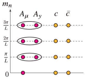
Figure 1: A schematic figure of the 4d spectrum of the abelian gauge field with ghosts on an interval. Each black oval pair indicates a QM-SUSY pair to make a mass term

2.2.2 4d spectrum of fermion

Second, we investigate the 4d spectrum of the fermion on an interval. The action and BCs are given by eq. (2.12) and eq. (2.29). To evaluate the 4d spectrum of the fermion, we expand the fermion as

$$\Psi(x,y) =\Psi_{R}(x,y)+\Psi_{L}(x,y)$$

$$=\sum_{n}\psi^{(n)}_{R}(x)\mathscr{F}^{(n)}_{\psi_{R}}(y)+\sum_{n}\psi^{(n)}_{L}(x)\mathscr{G}^{(n)}_{\psi_{L}}(y),$$ (2.64)

where $\{\mathscr{F}^{(n)}_{\psi_{R}}\}$ ($\{\mathscr{G}^{(n)}_{\psi_{L}}\}$) are eigenfunctions of the Hermitian operator $\mathscr{D}^{\dagger}\mathscr{D}$ ($\mathscr{D}\mathscr{D}^{\dagger}$):

$$\left\{\begin{array}[]{l}\mathscr{D}^{\dagger}\mathscr{D}\mathscr{F}^{(n)}_{\psi_{R}}(y)=m_{\psi^{(n)}}^{2}\mathscr{F}^{(n)}_{\psi_{R}}(y),\\[5.69046pt] \mathscr{D}\mathscr{D}^{\dagger}\mathscr{G}^{(n)}_{\psi_{L}}(y)=m_{\psi^{(n)}}^{2}\mathscr{G}^{(n)}_{\psi_{L}}(y),\end{array}\right.$$ (2.67)

and form complete sets. In the above, the operators $\mathscr{D}$ and $\mathscr{D}^{\dagger}$ are defined as

$$\mathscr{D} \equiv\partial_{y}+M_{F},$$ (2.68)

$$\mathscr{D}^{\dagger} \equiv-\partial_{y}+M_{F}.$$ (2.69)

Furthermore, $\{\mathscr{F}^{(n)}_{\psi_{R}}\}$ and $\{\mathscr{G}^{(n)}_{\psi_{L}}\}$ satisfy the QM-SUSY relations:

$$\left\{\begin{array}[]{l}\mathscr{D}\mathscr{F}^{(n)}_{\psi_{R}}(y)=m_{\psi^{(n)}}\mathscr{G}^{(n)}_{\psi_{L}}(y),\\[5.69046pt] \mathscr{D}^{\dagger}\mathscr{G}^{(n)}_{\psi_{L}}(y)=m_{\psi^{(n)}}\mathscr{F}^{(n)}_{\psi_{R}}(y).\end{array}\right.$$ (2.72)

We can obtain the explicit forms of the wavefunctions after we solve the eigenvalue equations (2.67) while taking into account the BCs (2.29). However, we here concentrate on the existence of a chiral massless zero-mode and the form of its wavefunction. Zero-mode solutions are obtained from the QM-SUSY relations (2.72) with $m_{\psi^{(0)}}=0$:

$$\mathscr{D}\mathscr{F}^{(0)}_{\psi_{R}} =0,$$ (2.73)

$$\mathscr{D}^{\dagger}\mathscr{G}^{(0)}_{\psi_{L}} =0.$$ (2.74)

The solutions of the above equations would be given as follows:

$$\mathscr{F}^{(0)}_{\psi_{R}}(y) =\sqrt{\frac{2M_{F}}{1-e^{-2M_{F}L}}}e^{-M_{F}y},$$ (2.75)

$$\mathscr{G}^{(0)}_{\psi_{L}}(y) =\sqrt{\frac{2M_{F}}{e^{2M_{F}L}-1}}e^{M_{F}y}.$$ (2.76)

Schematic figures of the zero-mode solutions are depicted in Figure 2. The zero-mode solution $\mathscr{F}^{(0)}_{\psi_{R}}$ $\Bigl{(}\mathscr{G}^{(0)}_{\psi_{L}}\Bigr{)}$ localizes to the boundary $y=0$ ($y=L$) in the case of $M_{F}>0$ and localizes to $y=L$ ($y=0$) in the case of $M_{F}<0$.

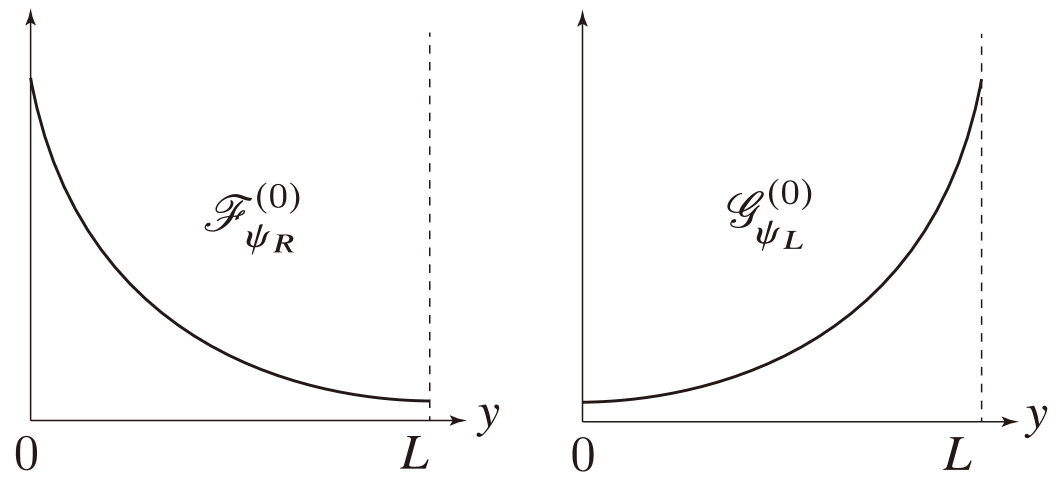
(i) Schematic figures of $\mathscr{F}^{(0)}_{\psi_{R}}$ and $\mathscr{G}^{(0)}_{\psi L}$ in the case of $M_{F}>0$. $\mathscr{F}^{(0)}_{\psi_{R}}$ ($\mathscr{G}^{(0)}_{\psi_{L}}$) localizes to the boundary point $y=0$ ($y=L$).

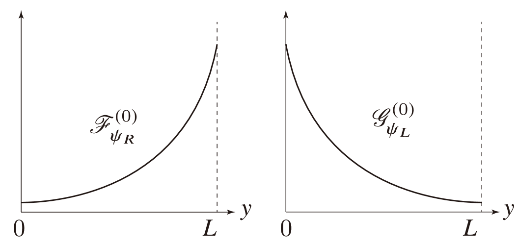
(ii) Schematic figures of $\mathscr{F}^{(0)}_{\psi_{R}}$ and $\mathscr{G}^{(0)}_{\psi_{L}}$ in the case of $M_{F}<0$. $\mathscr{F}^{(0)}_{\psi_{R}}$ ($\mathscr{G}^{(0)}_{\psi_{L}}$) localizes to the boundary point $y=L$ ($y=0$).

Figure 2: Schematic figures of chiral massless fermion zero mode solutions.

It should be emphasized that the zero-mode solutions $(\ref{f0R})$ $\bigl{(}(\ref{g0L})\bigr{)}$ are consistent only with the type-(II) $\bigl{(}$type-(I)$\bigr{)}$ BC given in (2.29) because of (2.23) and (2.24), respectively. Therefore we will concentrate on the type-(I) and type-(II) BCs in the following. The mass spectrum of both type-(I) and type-(II) is given by

$$m_{\psi^{(0)}} =0,$$ (2.77)

$${m_{\psi^{(n)}}} {=\sqrt{\left(\frac{n\pi}{L}\right)^{2}+M_{F}^{2}}},\hskip 40.00006pt(n=1,2,3,\cdots).$$ (2.78)

Inserting the mode expansions into the action and using the orthonormal relations of the mode functions, we have

$$S_{F}=\int d^{4}x\left\{{\cal L}_{m=0}+\sum^{\infty}_{n=1}\overline{\psi^{(n)}}(x)\Bigl{(}i\gamma^{\mu}\partial_{\mu}+m_{n}\Bigr{)}\psi^{(n)}(x)\right\},$$ (2.79)

where

$${\cal L}_{m=0} =\left\{\begin{array}[]{l}\overline{\psi^{(0)}_{L}}(x)(i\gamma^{\mu}\partial_{\mu})\psi^{(0)}_{L}(x),\hskip 40.00006pt\text{{for}\quad type-(I)},\\[8.5359pt] \overline{\psi^{(0)}_{R}}(x)(i\gamma^{\mu}\partial_{\mu})\psi^{(0)}_{R}(x),\hskip 40.00006pt\text{{for}\quad type-(II)},\end{array}\right.$$ (2.82)

and $\psi^{(n)}=\psi^{(n)}_{R}+\psi^{(n)}_{L}$. A typical spectrum of the fermion is depicted in Figure 3. A chiral massless zero mode exists in the case of both type-(I) and type-(II).

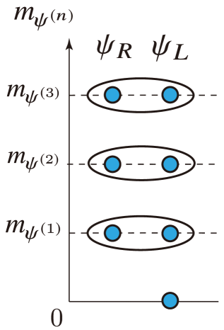
Type-(I) case

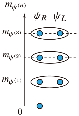
Type-(II) case

Figure 3: A typical mass spectrum of the fermion on an interval. Each black oval pair indicates a QM-SUSY pair to make a mass term.

2.2.3 Vacuum expectation value of the scalar

Finally, we comment on the vacuum expectation value of the scalar field. The action and the BCs are given by eq. (2.30) and eq. (2.38). It was found in Refs. [25, 26] that under the Robin boundary condition (2.38), $\Phi(x,y)$ can possess a non-vanishing vacuum expectation value $\langle\Phi(x,y)\rangle=\phi(y)$ with the form

$$\phi(y)=\dfrac{\frac{M}{\sqrt{\lambda}}(\sqrt{1+X}-1)^{\frac{1}{2}}}{{\rm cn}\left[M(1+X)^{\frac{1}{4}}(y-y_{0}),\sqrt{\frac{1}{2}(1+\frac{1}{\sqrt{1+X}}})\right]},$$ (2.83)

with

$$X=\frac{4\lambda|Q|}{M^{4}}.$$ (2.84)

${\rm cn}(y,a)$ is the Jacobi’s elliptic function, and $y_{0}$, $Q$ are constants which are determined by the parameters $L_{\pm}$ of the Robin BCs. Choosing suitable values of $L_{\pm}$, we can approximately take the form of the scalar VEV $\phi(y)$ as

$$\phi(y)\sim{\cal A}e^{My},$$ (2.85)

where ${\cal A}$ is a constant with mass dimension $\frac{3}{2}$.

3 Casimir energy and stability of the extra dimension

In the previous section, we succeeded in obtaining the 4d spectrum of the fields with the specified BCs. Taking the result into account, we evaluate the Casimir energy $E[L]$ as a function of the length $L$ of the extra dimension and show that the minimization of the Casimir energy provides a mechanism to stabilize the extra dimension.

For our purpose, we only concentrate on the gauge and fermion field contributions to the Casimir energy while ignoring the effect of the scalar field in this paper. We summarize the action and the BCs which we consider,

$$S =S_{G}+S_{F},$$ (3.1)

$$S_{G} =\int d^{4}x\int^{L}_{0}dy\Bigl{[}-\frac{1}{4}F^{MN}F_{MN}-\frac{1}{2}(\partial^{\mu}A_{\mu}+\partial_{y}A_{y})^{2}-i\bar{c}(\partial^{\mu}\partial_{\mu}+\partial_{y}^{2})c\Bigr{]},$$ (3.2)

$$S_{F} =\int d^{4}x\int^{L}_{0}dy\ \overline{\Psi}(i\Gamma^{\mu}\partial_{\mu}+i\Gamma^{y}\partial_{y}+M_{F})\Psi,$$ (3.3)

$$\left\{\begin{array}[]{l}\partial_{y}A_{\mu}=0,\\ A_{y}=0,\end{array}\right.\hskip 30.00005pt{\rm at}\ y=0,L{,}$$ (3.6)

$$\partial_{y}c=0=\partial_{y}\bar{c}\hskip 30.00005pt{\rm at}\ y=0,L,$$ (3.7)

$$\begin{array}[]{ll}\text{type-(I)}:\Psi_{R}(0)=0=\Psi_{R}(L),\\[5.69046pt] \text{type-(II)}:\Psi_{L}(0)=0=\Psi_{L}(L){.}\end{array}$$ (3.10)

We focus on the situation in which a chiral massless zero mode exists. As an example, we consider the type-(II) BC first. To evaluate the Casimir energy, we examine the partition function $Z[L]$.

$$Z[L]=\int[dA_{\mu}\,dA_{y}\,{d\Psi\,d\bar{\Psi}}\,dc\,d\bar{c}]\,e^{iS}.$$ (3.11)

The gauge field part of the partition function reads

$$Z_{G}[L] =\int[dA_{\mu}dA_{y}dcd\bar{c}]\,e^{iS_{G}}$$ (3.12)

$$\propto{\rm exp}\left[i\int d^{4}x\Biggl{\{}i\int\frac{d^{4}p}{(2\pi)^{4}}\,\biggl{(}{\rm ln}\,p^{\mu}p_{\mu}+\frac{3}{2}\sum^{\infty}_{n=1}{\rm ln}\,(p^{\mu}p_{\mu}+m_{n}^{2})\biggr{)}\Biggr{\}}\right].$$ (3.13)

After moving to the Euclidian space, we obtain the Casimir energy of the gauge field:

$$Z^{{\rm Euclid}}_{G}[L]\propto{\rm exp}\left[-E^{\rm U(1)}[L]\int d^{4}x_{E}\right],$$ (3.14)

where

$$E^{\rm U(1)}[L] =\int\frac{d^{4}p_{E}}{(2\pi)^{4}}\left[{\rm ln}\,p_{E}^{2}+\frac{3}{2}\sum^{\infty}_{n=1}{\rm ln}\,(p_{E}^{2}+m_{n}^{2})\right]$$

$$=\int\frac{d^{4}p_{E}}{(2\pi)^{4}}\left[\frac{1}{4}\,{\rm ln}\,p_{E}^{2}+\frac{3}{4}\sum^{\infty}_{n=-\infty}{\rm ln}\Bigl{\{}p_{E}^{2}+\left(\frac{n\pi}{L}\right)^{2}\Bigr{\}}\right].$$ (3.15)

and $p_{E}^{2}=(p^{0}_{E})^{2}+(p^{1}_{E})^{2}+(p^{2}_{E})^{2}+(p^{3}_{E})^{2}$. For further concrete discussions, we divide $E^{\rm U(1)}[L]$ into two parts:

$$E^{\rm U(1)}[L] =E^{\rm U(1)}_{{\rm part1}}[L]+E^{\rm U(1)}_{{\rm part2}}[L],$$ (3.16)

$$E^{\rm U(1)}_{{\rm part1}}[L] =\int\frac{d^{4}p_{E}}{(2\pi)^{4}}\ \frac{1}{4}\,{\rm ln}\,p_{E}^{2},$$ (3.17)

$$E^{\rm U(1)}_{{\rm part2}}[L] =\int\frac{d^{4}p_{E}}{(2\pi)^{4}}\ \frac{3}{4}\sum^{\infty}_{n=-\infty}{\rm ln}\,\biggl{\{}p_{E}^{2}+\left(\frac{n\pi}{L}\right)^{2}\biggr{\}}$$ (3.18)

Now we find that $E^{\rm U(1)}_{\rm part1}[L]$ has no $L$-dependence. Our interest is only in the $L$-dependence of the Casimir energy $E^{\rm U(1)}[L]$ so that we simply ignore this part. We emphasize that this part actually does not affect any results of the $L$-dependence of the Casimir energy $E^{\rm U(1)}[L]$. On the other hand, $E^{\rm U(1)}_{\rm part2}[L]$ has an $L$-dependence and plays a crucial role when we discuss the $L$-dependence of the total Casimir energy. By using the formulas

$$-{\rm ln}\,A=\frac{d}{ds}A^{-s}\biggr{|}_{s=0},$$ (3.19)

$$A^{-s}=\frac{1}{\Gamma(s)}\int^{\infty}_{0}dt\ t^{s-1}e^{-At},$$ (3.20)

$$\frac{d}{ds}\frac{t^{s}}{\Gamma(s)}\Biggr{|}_{s=0}=1,$$ (3.21)

with the Gamma function $\Gamma(s)=\int^{\infty}_{0}dt\,t^{s-1}e^{-t}$, we can rewrite $E^{\rm U(1)}_{\rm part2}[L]$ as

$$E^{\rm U(1)}_{\rm part2}[L]=-\frac{3}{4}\cdot\frac{1}{16\pi^{2}}\sum^{\infty}_{n=-\infty}\int^{\infty}_{0}dt\,t^{-3}e^{-(\frac{n\pi}{L})^{2}t}.$$ (3.22)

The Poisson summation formula

$$\sum^{\infty}_{n=-\infty}e^{-(\frac{n\pi}{L})^{2}t}=\sum^{\infty}_{w=-\infty}\frac{L}{\sqrt{\pi t}}e^{-\frac{w^{2}L^{2}}{t}},$$ (3.23)

will help us to move on. Here, the index $w$ is an integer which represents the winding number. By utilizing the Poisson summation formula, we obtain

$$E^{\rm U(1)}_{\rm part2}[L]=-\frac{3L}{64\pi^{5/2}}\sum^{\infty}_{w=-\infty}\int^{\infty}_{0}dt\,{t}^{-\frac{7}{2}}e^{-\frac{w^{2}L^{2}}{t}},$$ (3.24)

and find that $E^{\rm U(1)}_{\rm part2}[L]$ contains a UV-divergence when $t\rightarrow 0$. To remove this UV-divergence, we define the regularized total Casimir energy as

$$\frac{1}{L}E^{\rm U(1)}_{\rm part2}[L]_{\rm reg.}\equiv\frac{1}{L}E^{\rm U(1)}_{\rm part2}[L]-\frac{1}{L}E^{\rm U(1)}_{\rm part2}[L]\Biggr{|}_{{L\to\infty}}.$$ (3.25)

We note that this regularization is equivalent simply to removing the $w=0$ mode from the Casimir energy. The $w\neq 0$ modes express winding modes and provide finite contributions to the $L$-dependence of the Casimir energy. On the other hand, $w=0$ corresponds to an unwinding mode and it causes a UV-divergence. Since the regularized Casimir energy $E^{\rm U(1)}_{\rm part2}[L]_{\rm reg.}$ does not contain any unwinding mode, it has no UV-divergence and becomes finite. The explicit form of $E^{\rm U(1)}_{\rm part2}[L]$ is

$$E^{\rm U(1)}_{\rm part2}[L]_{\rm reg.} =-\frac{3L}{32\pi^{5/2}}\sum^{\infty}_{w=1}\int^{\infty}_{0}dt\,t^{-\frac{7}{2}}e^{-\frac{w^{2}L^{2}}{t}}$$

$$=-\frac{3L}{32\pi^{5/2}}\sum^{\infty}_{w=1}\frac{1}{w^{5}L^{5}}\int^{\infty}_{0}dt^{\prime}\ t^{\prime}{}^{\frac{5}{2}-1}e^{-t^{\prime}}$$

$$=-\frac{9}{128\pi^{2}L^{4}}\zeta(5),$$ (3.26)

where we performed the integration by substitution $t^{\prime}\equiv\frac{w^{2}L^{2}}{t}$ and used $\Gamma(\frac{5}{2})=\frac{3\sqrt{\pi}}{4}$. From the above analysis, we obtain the regularized Casimir energy $E^{\rm U(1)}[L]_{\rm reg.}$ of the gauge field:

$$E^{\rm U(1)}[L]_{\rm reg.}=-\frac{9}{128\pi^{2}L^{4}}\zeta(5).$$ (3.27)

In the same way, we next evaluate the Casimir energy of the fermion with the type-(II) boundary condition. (It is found that the type-(I) boundary condition leads to the same conclusion as the type-(II) for the Casimir energy.) To move on, we introduce the chiral representation:

$$\psi^{(n)}=\left(\begin{array}[]{c}\xi^{(n)}\\ 0\end{array}\right)+\left(\begin{array}[]{c}0\\ \eta^{(n)}\end{array}\right){.}$$ (3.32)

The Gamma matrices are represented by

$$\gamma^{\mu}=\left(\begin{array}[]{cc}0&\bar{\sigma}^{\mu}\\ \sigma^{\mu}&0\\ \end{array}\right),$$ (3.35)

where

$$\bar{\sigma}^{\mu} =(1,{\bm{\sigma}}),$$ (3.36)

$$\sigma^{\mu} =(1,-{\bm{\sigma}}){,}$$ (3.37)

and ${\bm{\sigma}}$ are Pauli matrices. The partition function of the fermion reads

$$Z_{F}[M_{F},L] =\int[{d\Psi d\bar{\Psi}}]\ e^{iS_{F}}$$

$$\propto{\rm exp}\left[i\int d^{4}x\Biggl{\{}-i\int\frac{d^{4}p}{(2\pi)^{4}}\,\biggl{(}{\rm ln}\,p^{\mu}p_{\mu}+2\sum^{\infty}_{n=1}{\rm ln}\,(p^{\mu}p_{\mu}+m_{\psi^{(n)}}^{2})\biggr{)}\Biggr{\}}\right]{,}$$ (3.38)

where the overall minus sign originates in the Grassmann property of fermions. After moving to the Euclidian space, we obtain the Casimir energy of the fermion:

$$Z^{\rm Euclid}_{F}[M_{F},L] \propto{\rm exp}\left[-E^{(F)}[M_{F},L]\int d^{4}x_{E}\right],$$ (3.39)

where

$$E^{(F)}[M_{F},L] =-\int\frac{d^{4}p_{E}}{(2\pi)^{4}}\left[{\rm ln}\,p_{E}^{2}+2\sum^{\infty}_{n=1}\,{\rm ln}(p_{E}^{2}+m_{\psi^{(n)}}^{2})\right]$$

$$=-\int\frac{d^{4}p_{E}}{(2\pi)^{4}}\left[{\rm ln}\,p_{E}^{2}-{\rm ln}\,(p_{E}^{2}+M_{F}^{2})+\sum^{\infty}_{n=-\infty}{\rm ln}\,\biggl{\{}p_{E}^{2}+\Bigl{(}\frac{n\pi}{L}\Bigr{)}^{2}+M_{F}^{2}\biggr{\}}\right].$$ (3.40)

We divide $E^{(F)}[M_{F},L]$ into two parts as is the case of the gauge field:

$$E^{(F)}[M_{F},L] =E^{(F)}_{\rm part1}[M_{F},L]+E^{(F)}_{\rm part2}[M_{F},L],$$ (3.41)

$$E^{(F)}_{\rm part1}[M_{F},L] =-\int\frac{d^{4}p_{E}}{(2\pi)^{4}}\left[{\rm ln}\,p_{E}^{2}-{\rm ln}\,(p_{E}^{2}+M_{F}^{2})\right],$$ (3.42)

$$E^{(F)}_{\rm part2}[M_{F},L] =-\int\frac{d^{4}p_{E}}{(2\pi)^{4}}\sum^{\infty}_{n=-\infty}{\rm ln}\,\left[p_{E}^{2}+\Bigl{(}\frac{n\pi}{L}\Bigr{)}^{2}+M_{F}^{2}\right].$$ (3.43)

In the same way as the gauge field, $E^{(F)}_{\rm part1}[M_{F},L]$ does not contain any $L$-dependence. Since we have an interest in the $L$-dependence of the Casimir energy, we just ignore this part. $E^{(F)}_{\rm part2}[M_{F},L]$ can be also evaluated as the gauge field case. Using the formulas (3.19)-(3.21), we can rewrite $E^{(F)}_{\rm part2}[M_{F},L]$ as

$$E^{(F)}_{\rm part2}[M_{F},L]=\frac{1}{16\pi^{2}}\sum^{\infty}_{n=-\infty}\int^{\infty}_{0}dt\,t^{-3}e^{-\left\{(\frac{n\pi}{L})^{2}+M_{F}^{2}\right\}t}.$$ (3.44)

By using the Poisson summation formula (3.23), we obtain the following form for $E^{(F)}_{\rm part2}[M_{F},L]$:

$$E^{(F)}_{\rm part2}[M_{F},L]=\frac{L}{16\pi^{5/2}}\sum^{\infty}_{w=-\infty}\int^{\infty}_{0}dt\,t^{-\frac{7}{2}}e^{-\frac{w^{2}L^{2}}{t}-M_{F}^{2}t}.$$ (3.45)

Since $E^{(F)}_{\rm part2}[M_{F},L]$ contains UV-divergence when $t\rightarrow 0$, we regularize it as

$$\frac{1}{L}E^{(F)}_{\rm part2}[M_{F},L]_{\rm reg.}\equiv\frac{1}{L}E^{(F)}_{\rm part2}[M_{F},L]-\frac{1}{L}E^{(F)}_{\rm part2}[M_{F},L]\Biggr{|}_{L\rightarrow\infty}.$$ (3.46)

The regularized Casimir energy $E^{(F)}_{\rm part2}[M_{F},L]_{\rm reg.}$ is expressed by the modified Bessel function $K_{\nu}(z)$ as

$$E^{(F)}_{\rm part2}[M_{F},L]_{\rm reg.}=\frac{{L}}{4\pi^{5/2}}\sum^{\infty}_{w=1}\left(\frac{|M_{F}|}{wL}\right)^{\frac{5}{2}}K_{\frac{5}{2}}(2w|M_{F}|L),$$ (3.47)

where the modified Bessel function is defined by

$$2\left(\frac{A}{B}\right)^{\frac{\nu}{2}}K_{\nu}(2\sqrt{AB})=\int^{\infty}_{0}dt\,t^{-\nu-1}e^{-At-\frac{B}{t}}.$$ (3.48)

Moreover, the modified Bessel function $K_{\frac{D}{2}}(z)$ with $D=\text{odd integer}$ can be expressed as

$$K_{\frac{D}{2}}(z)=\sqrt{\frac{\pi}{2z}}e^{-z}\sum^{\frac{D-1}{2}}_{k=0}\frac{\Bigl{(}\frac{D-1}{2}+k\Bigr{)}!}{k!\left(\frac{D-1}{2}-k\right)!(2z)^{k}}.$$ (3.49)

Therefore the explicit form of $E^{(F)}_{\rm part2}[M_{F},L]_{\rm reg.}$ is given by

$$E^{(F)}_{\rm part2}[M_{F},L]_{\rm reg.}=\frac{|M_{F}|^{2}}{8\pi^{2}L^{2}}\sum^{\infty}_{w=1}\frac{e^{-2w|M_{F}|L}}{w^{3}}\left(1+\frac{3}{2w|M_{F}|L}+\frac{3}{4w^{2}(|M_{F}|L)^{2}}\right).$$ (3.50)

From the analysis, we obtain the $L$-dependence of the regularized total Casimir energy $E^{(F)}[M_{F},L]_{\rm reg.}$ of the fermion as

$${E^{(F)}[M_{F},L]_{\rm reg.}=\frac{|M_{F}|^{2}}{8\pi^{2}L^{2}}\sum^{\infty}_{w=1}\frac{e^{-2w|M_{F}|L}}{w^{3}}\left(1+\frac{3}{2w|M_{F}|L}+\frac{3}{4w^{2}(|M_{F}|L)^{2}}\right).}$$ (3.51)

Schematic figures of the regularized Casimir energy of the fermion $E^{(F)}[M_{F},L]_{\rm reg.}$ and its derivative $\frac{d}{dL}E^{(F)}[M_{F},L]_{\rm reg.}$ are depicted in Figure 4 and Figure 5.

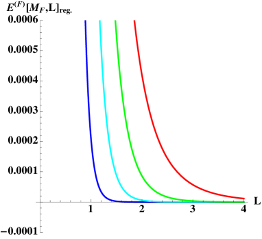
Figure 4: Schematic figure of the $L$-dependence of the Casimir energy $E^{(F)}[M_{F},L]_{\rm reg.}$. The blue, cyan, green, and red lines correspond to the cases of $M_{F}=3.5$, $M_{F}=2$, $M_{F}=1.1$, and $M_{F}=0.4$, respectively. In this plot, $M_{F}$ and $L$ should be regarded as dimensionless parameters by multiplying a fundamental scale of the theory.

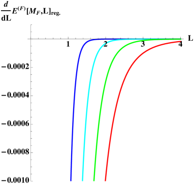
Figure 5: Schematic figure of the $L$-dependence of the derivative of the Casimir energy $\frac{d}{dL}E^{(F)}[M_{F},L]_{\rm reg.}$. The blue, cyan, green, and red lines correspond to the cases of $M_{F}=3.5$, $M_{F}=2$, $M_{F}=1.1$, and $M_{F}=0.4$, respectively. In this plot, $M_{F}$ and $L$ should be regarded as dimensionless parameters by multiplying a fundamental scale of the theory.

Combining all the results and concentrating on the $L$-dependence of the Casimir energy, we obtain the regularized Casimir energy $E[M_{F},L]_{\rm reg.}$ as

$$E[M_{F},L]_{\rm reg.} =E^{\rm U(1)}[L]_{\rm reg.}+E^{(F)}[M_{F},L]_{\rm reg.}$$

$$=-\frac{9}{128\pi^{2}L^{4}}\zeta(5){+\frac{|M_{F}|^{2}}{8\pi^{2}L^{2}}\sum^{\infty}_{w=1}\frac{e^{-2w|M_{F}|L}}{w^{3}}\left(1+\frac{3}{2w|M_{F}|L}+\frac{3}{4w^{2}(|M_{F}|L)^{2}}\right)}.$$ (3.52)

Schematic figures of the total Casimir energy $E[M_{F},L]_{\rm reg.}$ and its derivative $\frac{d}{dL}E[M_{F},L]_{\rm reg.}$ are depicted in Figure 6 and Figure 7. We can find that there exists a non-trivial global minimum to the Casimir energy. Thus we can conclude that the extra dimension is stable in this setup.

We should give a comment for the above results. It was discussed in ref. [29] that, in the case of $M_{F}=0$, the $L$-dependence of $E^{(F)}[M_{F},L]_{\rm reg.}$ becomes

$$E^{(F)}[M_{F},L]_{\rm reg.}\sim\dfrac{\alpha}{L^{4}}\quad(\alpha:\text{Const.}),$$ (3.53)

so that the finite global minimum does not appear in the Casimir energy. In the case of $M_{F}\neq 0$, the fermion’s positive contribution to the Casimir energy becomes dominant for $L\rightarrow 0$ because the fermion has more degrees of freedom than the gauge field. On the other hand, the negative contribution of the gauge field becomes dominant for $L\rightarrow\infty$ since the contribution of the fermion is suppressed by the exponential factor via the bulk mass. Therefore, we have revisited that the extra dimension can be stabilized if the following two conditions, which were pointed out in Ref. [29], are satisfied: (i) 5d massless gauge bosons exist and all 5d fermions have nonzero bulk masses; and (ii) the degrees of freedom of fermions are sufficiently larger than those of bosons. In our interval extra dimension case, in contrast with orbifold models, a bulk mass $M_{F}$ is not forbidden from any symmetry and should be involved so that the finite global minimum of the Casimir energy can emerge.

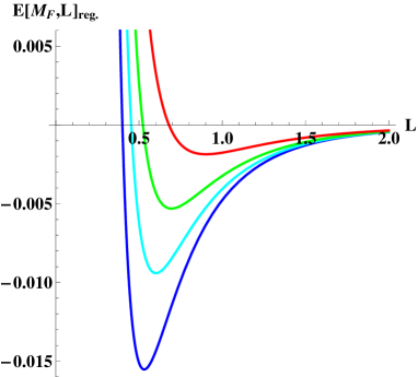
Figure 6: Schematic figure of the total Casimir energy $E[M_{F},L]_{\rm reg.}$ as a function of the length $L$ of the extra dimension. The blue, cyan, green, and red lines correspond to the cases of $M_{F}=1.7$, $M_{F}=1.5$, $M_{F}=1.3$, and $M_{F}=1$, respectively. In this plot, $M_{F}$ and $L$ should be regarded as dimensionless parameters by multiplying a fundamental scale of the theory. We can find a non-trivial global minimum and can conclude that the extra dimension is stable.

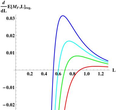
Figure 7: Schematic figure of the derivative of the total Casimir energy $\frac{d}{dL}E[M_{F},L]_{\rm reg.}$ as a function of the length $L$ of the extra dimension. The blue, cyan, green, and red lines correspond to the case of $M_{F}=1.7$, $M_{F}=1.5$, $M_{F}=1.3$, and $M_{F}=1$, respectively. In this plot, $M_{F}$ and $L$ should be regarded as dimensionless parameters by multiplying a fundamental scale of the theory. We can find a non-trivial global minimum.

4 Theory with point interactions

In the papers [26, 27, 28, 52], a new way to produce generations and a mass hierarchy was proposed with introducing zero-width branes, so-called point interactions, to the extra dimension. In this section, we briefly review a theory with point interactions at first. In the theory, massless zero modes become degenerate and a nontrivial number of generations appears from a one-generation 5d fermion (where a self-contained comprehensive review on the formulation is provided in Appendix A). In this section, we clarify the 4d mass spectrum of the theory with point interactions, which plays an important role in the calculation of the Casimir energy.

4.1 BCs and 4d mass spectrum

In a theory with point interactions, we can recognize the point interactions as extra boundary points and need to impose extra boundary conditions at the points. Assuming that only the fermion feels the point interactions at $y=L_{1},\,L_{2}$, we can obtain three-generation chiral massless zero modes from the following BCs :

$$\Psi_{R}(y) =0\qquad\text{at}\qquad{y=0,\,L_{1}{\pm\varepsilon},\,L_{2}{\pm\varepsilon},\,L},$$ (4.1)

or

$$\Psi_{L}(y) =0\qquad\text{at}\qquad{y=0,\,L_{1}{\pm\varepsilon},\,L_{2}{\pm\varepsilon},\,L},$$ (4.2)

where $\varepsilon$ represents an infinitesimal positive constant. We should emphasize that the above BCs are consistent with the 5d gauge invariance since they are invariant under the 5d gauge transformation:

$$\Psi_{R}(x,y)\ \rightarrow\ \widetilde{\Psi}_{R}(x,y)=e^{-ig\Lambda(x,y)}\Psi_{R}(x,y),$$ (4.3)

$$\Psi_{L}(x,y)\ \rightarrow\ \widetilde{\Psi}_{L}(x,y)=e^{-ig\Lambda(x,y)}\Psi_{L}(x,y).$$ (4.4)

We expand a 5d fermion $\Psi(x,y)$ with the BCs (4.1) or (4.2):

$${\Psi(x,y)=\Psi_{R}(x,y)+\Psi_{L}(x,y)=\sum_{n}\psi^{(n)}_{R}(x)\mathscr{F}^{(n)}_{\psi_{R}}(y)+\sum_{n}\psi^{(n)}_{L}(x)\mathscr{G}^{(n)}_{\psi_{L}}(y).}$$ (4.5)

It was found in Refs. [26, 27, 28] that we have three degenerate zero modes $\mathscr{G}^{(0)}_{i,\psi_{L}}(y)$ with $i=1,2,3$ $\bigl{(}\mathscr{F}^{(0)}_{i,\psi_{R}}$ with $i=1,2,3\bigr{)}$ under the BC (4.1) $\bigl{(}$the BC (4.2)$\bigr{)}$ and can obtain three degenerate massless chiral fermions $\psi_{i,L}^{(0)}(x)$ $\bigl{(}\psi_{i,R}^{(0)}(x)\bigr{)}$:

$$\Psi(x,y) =\Psi_{0}(x,y)+\sum_{n=1}^{\infty}\sum^{{3}}_{i=1}\left\{{\psi^{(n)}_{i,R}(x)}\mathscr{F}^{(n)}_{i,\psi_{R}}(y)+{\psi^{(n)}_{i,L}(x)}\mathscr{G}_{i,\psi_{L}}^{(n)}(y)\right\},$$ (4.6)

$$\Psi_{0}(x,y) =\left\{\begin{array}[]{l}\displaystyle\sum^{{3}}_{i=1}{\psi^{(0)}_{i,L}(x)}\mathscr{G}_{i,\psi_{L}}^{(0)}(y),\qquad\text{{for}}\quad\Psi_{R}(y)=0\quad\text{at}\quad{y=0,\,L_{1}{\pm\varepsilon},\,L_{2}{\pm\varepsilon},\,L},\\ \displaystyle\sum^{{3}}_{i=1}{\psi^{(n)}_{i,R}(x)}\mathscr{F}_{i,\psi_{R}}^{(0)}(y),\qquad\text{{for}}\quad\Psi_{L}(y)=0\quad\text{at}\quad{y=0,\,L_{1}{\pm\varepsilon},\,L_{2}{\pm\varepsilon},\,L},\end{array}\right.$$ (4.9)

where $\mathscr{G}_{i,\psi_{L}}^{(0)}(y)$ $\bigl{(}\mathscr{F}_{i,\psi_{R}}^{(0)}(y)\bigr{)}$ is a solution of eq. (2.74) $\bigl{(}$eq. (2.73)$\bigr{)}$ under the BC (4.1) with eq. (2.23) $\bigl{(}$the BC (4.2) with eq. (2.24)$\bigr{)}$. The explicit forms of $\mathscr{G}_{i,\psi_{L}}^{(0)}(y)$ and $\mathscr{F}_{i,\psi_{R}}^{(0)}(y)$ are given by

$$\mathscr{G}_{i,\psi_{L}}^{(0)}(y) =\sqrt{\frac{2M_{F}}{e^{2M_{F}l_{i}}-1}}e^{M_{F}(y-L_{i-1})}\Bigl{[}\theta(y-L_{i-1})\theta(L_{i}-y)\Bigr{]}$$ (4.10)

$$\mathscr{F}_{i,\psi_{R}}^{(0)}(y) =\sqrt{\frac{2M_{F}}{1-e^{-2M_{F}l_{i}}}}e^{-M_{F}(y-L_{i-1})}\Bigl{[}\theta(y-L_{i-1})\theta(L_{i}-y)\Bigr{]}$$ (4.11)

where

$${l_{i}\equiv L_{i}-L_{i-1}\quad(i=1,2,3;\ L_{3}=L,L_{0}=0)},$$ (4.12)

and $\theta(y)$ is the step function. Schematic figures of the localized zero modes $\mathscr{G}_{i,\psi_{L}}^{(0)}(y)$ and $\mathscr{F}_{i,\psi_{R}}^{(0)}(y)$ are depicted in Figure 8 and Figure 9. Each zero mode only lives in a segment and localizes to a boundary.

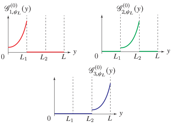
Figure 8: Schematic figures of localized zero modes $\mathscr{G}^{(0)}_{i,\psi_{L}}(y)$ ($i=1,2,3$) with $M_{F}>0$. Each zero mode of $\mathscr{G}^{(0)}_{i,\psi_{L}}(y)$ only has a non-vanishing value within the segment $L_{i-1}<y<L_{i}$ and localizes to a boundary.

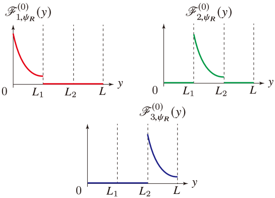
Figure 9: Schematic figures of localized zero modes $\mathscr{F}^{(0)}_{i,\psi_{R}}(y)$ ($i=1,2,3$) with $M_{F}>0$. Each zero mode of $\mathscr{F}^{(0)}_{i,\psi_{R}}(y)$ only has a non-vanishing value within the segment $L_{i-1}<y<L_{i}$ and localizes to a boundary.

After substituting eq. (4.6) into the action (2.12) and using the orthonormal relations

$$\int^{L}_{0}dy\,{\bigl{(}\mathscr{F}^{(n)}_{i,\psi_{R}}(y)\bigr{)}^{\ast}}\mathscr{F}^{(m)}_{j,\psi_{R}}(y) =\delta_{n,m}\delta_{i,j},$$ (4.13)

$$\int^{L}_{0}dy\,{\bigl{(}\mathscr{G}^{(n)}_{i,\psi_{L}}(y)\bigr{)}^{\ast}}\mathscr{G}^{(m)}_{j,\psi_{L}}(y) =\delta_{n,m}\delta_{i,j},\quad{(i,j=1,2,3)}$$ (4.14)

we obtain the 4d spectrum of the fermion,

$$S_{F}=\int d^{4}x\left\{{\cal L}_{n=0}+\sum_{n=1}^{\infty}{\sum^{3}_{i=1}}\ \bar{\psi}^{(n)}_{i}(i\gamma^{\mu}\partial_{\mu}+m_{i,\psi^{(n)}})\psi^{(n)}_{i}\right\},$$ (4.15)

where

$${\cal L}_{n=0}=\left\{\begin{array}[]{l}\displaystyle{\sum^{3}_{i=1}}\ \psi^{(0)}_{i,L}{(x)}(i\gamma^{\mu}\partial_{\mu})\psi^{(0)}_{i,L}{(x)}\qquad\text{for the {BC (\ref{RBC})}},\\ \displaystyle{\sum^{3}_{i=1}}\ \psi^{(0)}_{i,R}{(x)}(i\gamma^{\mu}\partial_{\mu})\psi^{(0)}_{i,R}{(x)}\qquad\text{for the {BC (\ref{LBC})}}.\end{array}\right.$$ (4.18)

and the 4d mass spectrum $m_{i,\psi^{(n)}}$ is given by

$$m_{i,\psi^{(n)}}={\sqrt{M_{F}^{2}+\left(\frac{n\pi}{l_{i}}\right)^{2}}}\qquad{({i=1,2,3;}\ n=1,2,3,\cdots)},$$ (4.19)

where $l_{i}$ is defined by eq. (4.12).

5 Dynamical generation of fermion mass hierarchy

In this section, by using the previous results, we consider an $SU(2)\times U(1)$ model with a single generation of 5d fermions, which produces three generations of 4d chiral fermions by the point interactions, and discuss whether the model can dynamically generate a fermion mass hierarchy. To this end, we first set an action and BCs of this model. The action consists of an $SU(2)$ gauge field, a $U(1)$ gauge field, a single generation $SU(2)$ doublet fermion, a single generation $SU(2)$ singlet fermion, and an $SU(2)$ doublet scalar field. The contents of our model mimic those of the SM without the color degree of freedom, where the $U(1)$ (hyper)charges of $Q$ and $U$ take those of the quark doublet and the up-type singlet. Extra BCs via point interactions are a key ingredient to produce the three generations from one generation 5d fermion as we reviewed in Section 4. The positions of the point interactions crucially affect the fermion mass hierarchy through the overlap integrals, as we will see in Section 5.3. We will show that the positions of the point interactions can be determined dynamically through the minimization of the Casimir energy and then find that an exponential fermion mass hierarchy naturally appears. Following the results, we discuss the stability of the extra dimension.

5.1 Action and BCs

We start with the following action for the gauge fields and fermions:

$$S =S_{G}+S_{F},$$ (5.1)

$$S_{G} =\int d^{4}x\int^{L}_{0}dy\left[-\frac{1}{4}W^{aMN}W_{MN}^{a}-\frac{1}{2}(\partial^{M}W_{M}^{a})^{2}-i\,\bar{c}^{a}(\partial^{M}{\cal D}_{M})c^{a}\right.$$

$$\hskip 100.00015pt\left.{-\frac{1}{4}F^{MN}F_{MN}-\frac{1}{2}(\partial^{M}A_{M})^{2}-i\bar{c}(\partial^{M}\partial_{M})c}\right],$$ (5.2)

$$S_{F} =\int d^{4}x\int^{L}_{0}dy\left[\bar{Q}\Bigl{(}i\Gamma^{M}D_{M}^{(Q)}+M_{F}^{(Q)}\Bigr{)}Q+{\bar{U}\Bigl{(}i\Gamma^{M}\partial_{M}+M_{F}^{(U)}\Bigr{)}U}\right],$$ (5.3)

where

$$W^{a}_{MN} =\partial_{M}W_{N}^{a}-\partial_{N}W_{M}^{a}{-g\varepsilon_{abc}W_{M}^{b}W_{N}^{c}},$$ (5.4)

$${F_{MN}} {=\partial_{M}A_{N}-\partial_{N}A_{M},}$$ (5.5)

$${\cal D}_{M}c^{a} =\partial_{M}c^{a}+g\varepsilon_{abc}W^{b}_{M}c^{c},$$ (5.6)

$$D_{M}^{(Q)}Q =\biggl{(}\partial_{M}{-igW_{M}^{a}T_{a}{-ig^{\prime}A_{M}}}\biggr{)}Q.$$ (5.7)

$W_{M}^{a}$, $A_{M}$, $c^{a}$, $c$ and $\bar{c}^{a}$, $\bar{c}$ denote an $SU(2)$ gauge, a $U(1)$ gauge, ghost and anti-ghost fields, respectively. $g$ and $g^{\prime}$ denote $SU(2)$ and $U(1)$ couplings of the $SU(2)$ doublet fermion. $Q$ and $U$ indicate an $SU(2)$ doublet fermion and an $SU(2)$ single fermion, respectively. A bulk mass of the 5d fermion is denoted by $M_{F}^{(\Psi)}$ ($\Psi=Q,{U}$). $\varepsilon_{abc}$ is a complete antisymmetric tensor and $T_{a}$ is a generator of $SU(2)$ acts on a fundamental representation, which satisfies the following algebra and the orthogonal relation:

$$[T_{a},T_{b}]=i\varepsilon_{abc}T_{c},$$ (5.8)

$$\text{tr}\,T_{a}T_{b}=\frac{1}{2}\delta_{a,b}.$$ (5.9)

According to the analysis given in Section 2, we choose boundary conditions for the fields as follows:

$$\left\{\begin{array}[]{l}\partial_{y}W_{\mu}^{a}(x,y)=0,\\ W_{y}^{a}(x,y)=0,\end{array}\right.\hskip 20.00003pt\text{at}\qquad y=0,L,$$ (5.12)

$$\left\{\begin{array}[]{l}{\partial_{y}c^{a}(x,y)=0},\\ {\partial_{y}\bar{c}^{a}(x,y)=0},\end{array}\right.\hskip 30.00005pt\text{at}\qquad y=0,L,$$ (5.15)

$${\left\{\begin{array}[]{l}\partial_{y}A_{\mu}(x,y)=0,\\ A_{y}(x,y)=0,\end{array}\right.\hskip 20.00003pt\text{at}\qquad y=0,L,}$$ (5.18)

$${\left\{\begin{array}[]{l}\partial_{y}c(x,y)=0,\\ \partial_{y}\bar{c}(x,y)=0,\end{array}\right.\hskip 30.00005pt\text{at}\qquad y=0,L,}$$ (5.21)

$$Q_{R}(x,y)=0\hskip 50.00008pt\text{at}\qquad y=0,L_{1}{\pm\varepsilon},L_{2}{\pm\varepsilon},L,$$ (5.22)

$${U_{L}(x,y)}=0\hskip 50.00008pt\text{at}\qquad y=0,L_{1}{\pm\varepsilon},L_{2}{\pm\varepsilon},L{,}$$ (5.23)

where $L_{1}$ and $L_{2}$ ($0<L_{1}<L_{2}<L$) denote the positions of the point interactions and $\varepsilon$ represents an infinitesimal positive constant. A schematic figure of the extra dimension is depicted in Figure 10. We introduced two point interactions at $y=L_{1}$ and $L_{2}$ for the fermions and put the situation that all fermions feel the point interactions at the same positions for simplicity. On the other hand, the gauge and the ghost fields are assumed not to feel the point interactions at $y=L_{1}$ and $L_{2}$. We note that the 5d gauge symmetries are intact under the configuration of the boundary conditions.

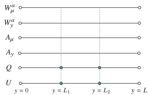
Figure 10: A schematic figure of the extra dimension. Only the fermions $Q$ and $U$ feel the point interactions (Green dots) at $y=L_{1},L_{2}$ and the gauge fields $W_{\mu}^{a}$, $W_{y}^{a}$, $A_{\mu}$ and $A_{y}$ do not. The situation is completely consistent with 5d gauge invariance.

5.2 Determination of the positions of the point interactions

Using the results of section 3, we can evaluate the Casimir energy as a function of the positions of the point interactions $\{L_{1},L_{2}\}$:

$${E^{{(F)}}[M^{(Q)}_{F},M^{{(U)}}_{F},L_{1},L_{2},L]_{\rm reg.}}$$

$${=} \,2\cdot\frac{|M^{(Q)}_{F}|^{2}}{8\pi^{2}L_{1}^{2}}\sum^{\infty}_{w=1}\frac{{\rm e}^{-2w|M^{(Q)}_{F}|L_{1}}}{w^{3}}\left(1+\frac{3}{2w|M_{F}^{(Q)}|L_{1}}+\frac{3}{4w^{2}|M_{F}^{(Q)}|^{2}L_{1}^{2}}\right)$$

$$+2\cdot\frac{|M_{F}^{(Q)}|^{2}}{8\pi^{2}(L_{2}-L_{1})^{2}}\sum^{\infty}_{w=1}\frac{{\rm e}^{-2w|M_{F}^{(Q)}|(L_{2}-L_{1})}}{w^{3}}\left(1+\frac{3}{2w|M_{F}^{(Q)}|(L_{2}-L_{1})}+\frac{3}{4w^{2}|M_{F}^{(Q)}|^{2}(L_{2}-L_{1})^{2}}\right)$$

$$+2\cdot\frac{|M_{F}^{(Q)}|^{2}}{8\pi^{2}(L-L_{2})^{2}}\sum^{\infty}_{w=1}\frac{{\rm e}^{-2w|M_{F}^{(Q)}|(L-L_{2})}}{w^{3}}\left(1+\frac{3}{2w|M_{F}^{(Q)}|(L-L_{2})}+\frac{3}{4w^{2}|M_{F}^{(Q)}|^{2}(L-L_{2})^{2}}\right)$$

$$+\frac{|M^{{(U)}}_{F}|^{2}}{8\pi^{2}L_{1}^{2}}\sum^{\infty}_{w=1}\frac{{\rm e}^{-2w|M^{{(U)}}_{F}|L_{1}}}{w^{3}}\left(1+\frac{3}{2w|M^{{(U)}}_{F}|L_{1}}+\frac{3}{4w^{2}{|M^{{(U)}}_{F}|}^{2}L_{1}^{2}}\right)$$

$$+\frac{|M^{{(U)}}_{F}|^{2}}{8\pi^{2}(L_{2}-L_{1})^{2}}\sum^{\infty}_{w=1}\frac{{\rm e}^{-2w|M^{{(U)}}_{F}|(L_{2}-L_{1})}}{w^{3}}\left(1+\frac{3}{2w|M^{{(U)}}_{F}|(L_{2}-L_{1})}+\frac{3}{4w^{2}|M^{{(U)}}_{F}|^{2}(L_{2}-L_{1})^{2}}\right)$$

$$+\frac{|M^{{(U)}}_{F}|^{2}}{8\pi^{2}(L-L_{2})^{2}}\sum^{\infty}_{w=1}\frac{{\rm e}^{-2w|M^{{(U)}}_{F}|(L-L_{2})}}{w^{3}}\left(1+\frac{3}{2w|M^{{(U)}}_{F}|(L-L_{2})}+\frac{3}{4w^{2}|M^{{(U)}}_{F}|^{2}(L-L_{2})^{2}}\right).$$ (5.24)

With the fixed length $L$, the minimization condition for the Casimir energy can determine the values of the parameters $\{L_{1},L_{2}\}$. The above potential turns out to have the finite global minimum at $L_{1}=\frac{L}{3}$, $L_{2}=\frac{2L}{3}$. To verify this statement, we consider the following function $I(x,y,z)$:

$$I(x,y,z)=f(x)+f(y)+f(z),$$ (5.25)

$${x,y,z>0},$$ (5.26)

$$x+y+z=1.$$ (5.27)

$I(x,y,z)$ imitates the function form of the fermion Casimir energy with the variables $x=\widetilde{L}_{1}$, $y=\widetilde{L}_{2}-\widetilde{L}_{1}$, $z=1-\widetilde{L}_{2}$, where $\widetilde{L}_{i}$ ($i=1,2$) is defined as $\widetilde{L}_{i}\equiv L_{i}/L$. We assume the function $f(x)$ to be a monotonically decreasing function and also $f^{\prime}(x)\equiv\dfrac{df(x)}{dx}$ to be a monotonically increasing one with $\displaystyle{\lim_{x\to 0}}f(x)=+\infty$. We note that the fermion Casimir energy (3.51) turns out to satisfy those assumptions (see Figures 4 and 5). Substituting the condition eq. (5.27) into eq. (5.25), we obtain

$$I(x,y,1-x-y)=f(x)+f(y)+f(1-x-y).$$ (5.28)

To investigate an extreme value of the above function, we examine $\dfrac{\partial I}{\partial x}$ and $\dfrac{\partial I}{\partial y}$:

$$\frac{\partial I}{\partial x} =f^{\prime}(x)-f^{\prime}(1-x-y),$$ (5.29)

$$\frac{\partial I}{\partial y} =f^{\prime}(y)-f^{\prime}(1-x-y),$$ (5.30)

From the conditions $\dfrac{\partial I}{\partial x}=0$ and $\dfrac{\partial I}{\partial y}=0$, we obtain the result

$$f^{\prime}(x)=f^{\prime}(y)=f^{\prime}(1-x-y){.}$$ (5.31)

Since we assumed that $f^{\prime}(x)$ is a monotonically increasing function, the result (5.31) can be realized only when

$$x=y=z=\frac{1}{3}.$$ (5.32)

Thus we find that $I(x,y,z)$ has an extreme value when $x=y=z=\dfrac{1}{3}$. Moreover, the function takes a local minimum at $x=y=z=\dfrac{1}{3}$. To show this, we consider the second-order differentials with the condition $x=y=z=\dfrac{1}{3}$:

$$\frac{\partial^{2}I}{\partial x^{2}}\biggr{|}_{x=y=\frac{1}{3}}=2f^{\prime\prime}\Bigl{(}\frac{1}{3}\Bigr{)},$$ (5.33)

$$\frac{\partial^{2}I}{\partial y\partial x}\biggr{|}_{x=y=\frac{1}{3}}=f^{\prime\prime}\Bigl{(}\frac{1}{3}\Bigr{)},$$ (5.34)

$$\frac{\partial^{2}I}{\partial x\partial y}\biggr{|}_{x=y=\frac{1}{3}}=f^{\prime\prime}\Bigl{(}\frac{1}{3}\Bigr{)},$$ (5.35)

$$\frac{\partial^{2}I}{\partial y^{2}}\biggr{|}_{x=y=\frac{1}{3}}=2f^{\prime\prime}\Bigl{(}\frac{1}{3}\Bigr{)}.$$ (5.36)

We now consider the Hessian matrix $M$:

$$M=\left(\begin{array}[]{cc}\dfrac{\partial^{2}I}{\partial x^{2}}\biggl{|}_{x=y=\frac{1}{3}}&\dfrac{\partial^{2}I}{\partial x\partial y}\biggl{|}_{x=y=\frac{1}{3}}\\[5.69046pt] \dfrac{\partial^{2}I}{\partial y\partial x}\biggl{|}_{x=y=\frac{1}{3}}&\dfrac{\partial^{2}I}{\partial y^{2}}\biggl{|}_{x=y=\frac{1}{3}}\end{array}\right)=\left(\begin{array}[]{cc}2f^{\prime\prime}\Bigl{(}\frac{1}{3}\Bigr{)}&f^{\prime\prime}\Bigl{(}\frac{1}{3}\Bigr{)}\\ f^{\prime\prime}\Bigl{(}\frac{1}{3}\Bigr{)}&2f^{\prime\prime}\Bigl{(}\frac{1}{3}\Bigr{)}\end{array}\right).$$ (5.41)

Since $f^{\prime}(x)$ is a monotonically increasing function, $f^{\prime\prime}(x)>0$. Thus we find that

$${\rm tr}\,M>0,$$ (5.42)

$${\rm det}\,M>0.$$ (5.43)

The above results imply that the eigenvalues of the matrix $M$ are positive and hence that the position $x=y=\dfrac{1}{3}$ is a local minimum of the potential. Moreover, there is no other stationary point, we found that the position $x=y=\dfrac{1}{3}$ is a global minimum of the function $I(x,y,z)$. From the above discussions, we conclude that the Casimir energy (5.24) has a global minimum at $L_{1}=\frac{L}{3}$, $L_{2}=\frac{2L}{3}$.

5.3 Fermion mass hierarchy

Under the above situation, we can produce the fermion mass hierarchy dynamically by introducing the Yukawa coupling to an $SU(2)$ doublet scalar field $\Phi(x,y)$, which possesses the y-dependent VEV

$${\langle\Phi(y)\rangle} {=\left(\begin{array}[]{c}\phi(y)\\ 0\end{array}\right),}$$ (5.46)

$${\phi(y)} {={\cal A}e^{My}},$$ (5.47)

as in eq. (2.85) because of the Robin boundary condition (2.38). The situation, in which the $i$-th generation ($i=1,2,3$) fermion lives in the segment $y\in[L_{i-1},L_{i}]$ ($L_{0}\equiv 0,L_{3}\equiv L$) and the scalar field lives in every region, makes a large mass hierarchy for the fermion masses through the Yukawa interaction $\lambda\bar{Q}\Phi{U}$:

$$m_{i}=\lambda\int^{L}_{0}dy\,{\bigl{(}\mathscr{G}^{(0)}_{i,Q_{L}}(y)\bigr{)}^{\ast}}{\phi(y)}\mathscr{F}^{(0)}_{i,{{U_{R}}}}(y){,}\qquad{(i=1,2,3)}$$ (5.48)

A schematic figure is depicted in Figure 11. Since the minimization of the Casimir energy determines the positions of the point interactions as to make the distances between them equal, the exponential VEV of the scalar field makes an exponential mass hierarchy such as

$${\frac{m_{2}}{m_{1}}=\frac{m_{3}}{m_{2}}={e^{\frac{1}{3}ML}}.}$$ (5.49)

Thus, the fermion mass hierarchy around $10^{5}$ can be obtained by suitably choosing the parameter $ML$. We emphasize that this mass hierarchy appears dynamically since the positions of the point interactions and the form of the VEV of the scalar are determined dynamically.

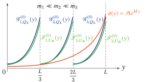
Figure 11: Schematic figure of zero mode profiles of chiral massless fermions and the VEV of the scalar field $\phi(y)$. The figure is depicted with the situation $M_{F}^{(Q)}>0$ and $M_{F}^{{(U)}}<0$. The position of the point interactions are fixed by the minimization of the Casimir energy and the $y$-dependent scalar VEV produces an exponential mass hierarchy through the overlap integrals with respect to the extra dimension.

5.4 Stability of the extra dimension

We have shown that for any fixed length $L$, the positions of the point interactions are determined dynamically to the value $L_{1}=\frac{L}{3}$, $L_{2}=\frac{2L}{3}$ from the minimization of the Casimir energy. Under this situation, we discuss the stability of the whole extra dimension. In our model the $SU(2)$ doublet scalar field $\Phi(x,y)$ possesses the y-dependent VEV and breaks the gauge symmetry as $SU(2)\times U(1)\to U(1)^{\prime}$. Therefore, we will discuss the stability of the extra dimension in the broken phase.

As we investigated in Section 3, the extra dimension can be stabilized if the following two conditions are satisfied: (i) 5d massless gauge bosons exist and all 5d fermions have nonzero bulk masses. (ii) The degrees of freedom of fermions are sufficiently larger than those of bosons. The first condition (i) will ensure that the Casimir energy approaches to zero with negative values in $L\to\infty$ limit, as in (3.42). The second condition (ii) will ensure that the Casimir energy goes to $+\infty$ in $L\to 0$ limit, as in (3.42).

In our model, the $SU(2)\times U(1)$ gauge symmetry is broken by the VEV of the scalar but a subgroup $U(1)^{\prime}$ is still unbroken. Thus, the first condition (i) is satisfied in our model. The second condition (ii) seems to be satisfied in our model because the degrees of freedom of the fermions become three times the number of 5d fermions due to the point interactions. Moreover, there is still room for introducing extra fermions by using the type-(III) BCs, which do not produce any exotic chiral massless fermions. Therefore, in our setup, the extra dimension is expected to be stabilized by the Casimir energy.

6 Conclusion and Discussion

In this paper, we proposed a new mechanism to produce a fermion mass hierarchy dynamically by introducing the point interactions to the 5d gauge theory on an interval. The interval extra dimension can possibly be stable and the point interactions produce generations of fermions. The positions of the point interactions were determined by minimizing the Casimir energy of the fermions. The extra-dimension coordinate-dependent VEV of the scalar field, which is also produced dynamically under the Robin boundary condition, makes exponentially different fermion masses through the overlap integrals.

We give a comment for the contribution of the scalar field to the Casimir energy at first. In this paper, we ignored the effect of the scalar field to the Casimir energy for simplicity because the contribution to the Casimir energy from the scalar field will have no exact analytic expression due to the Robin BC. However, the inclusion of the scalar field will not change the conclusions about the stability of the whole extra dimension and the positions of the point interactions if the degrees of freedom of the fermions are sufficiently larger than those of bosons.

Next, some comments are given to the flavor mixing of the fermions. In our model, we introduced the point interactions at $y=L_{1},L_{2}$ for both the $SU(2)$ doublet and the singlet fermions. Here, mass matrices are diagonal and flavor mixing cannot appear. In general, however, there is no need to share the point interactions in fermions so that we can introduce the individual point interactions to each fermion, respectively, which means that (e.g.) the $SU(2)$ doublet fermion feels the point interactions at $y=L_{1},L_{2}$ and the $SU(2)$ singlet fermion feels the point interactions at $y=L^{\prime}{}_{1},L^{\prime}{}_{2}$ [26, 27, 28]. Then the mode functions of the $SU(2)$-doublet zero mode $\mathscr{G}^{(0)}_{i,Q_{L}}(y)$ and the $SU(2)$-singlet zero mode $\mathscr{F}^{(0)}_{j,{{U_{R}}}}(y)$ may have an overlap for $i\neq j$. In other words, off diagonal components may appear in the mass matrix as

$$m_{ij}=\lambda\int^{L}_{0}dy\,{\Bigl{(}\mathscr{G}^{(0)}_{i,Q_{L}}(y)\Bigr{)}^{\ast}}{\phi(y)}\mathscr{F}^{(0)}_{j,{{U_{R}}}}(y),\qquad{(i,j=1,2,3)}$$ (6.1)

and a flavor mixing can be realized.

If the minimization of the Casimir energy determines the positions of the point interactions as $L_{1}=L^{\prime}{}_{1}$, $L_{2}=L^{\prime}{}_{2}$, flavor mixing does not appear so that we need an idea to make $L_{1}\neq L^{\prime}{}_{1}$, $L_{2}\neq L^{\prime}{}_{2}$. One way to avoid the situation of $L_{i}=L^{\prime}{}_{i}$ is to consider higher loop effects of the Casimir energy, which may make $L_{1}\neq L^{\prime}{}_{1}$, $L_{2}\neq L^{\prime}{}_{2}$ through the interactions. To introduce exotic 5d fermions, where they contribute to the Casimir energy, is another way. No chiral massless zero modes appear in an exotic fermion when we assign a suitable choice of boundary conditions to it. Under such conditions, the low energy matter contents of the model, i.e. the Standard Model particles, do not have a change. If we put a different boundary condition to $y=L_{1}$ ($y=L^{\prime}_{1}$) from $y=L_{2}$ ($y=L^{\prime}_{2}$), each segment has a different contribution of the Casimir energy so that we may produce the flavor mixing. A different strategy is to introduce more than two point interactions, e.g. $N-1$ point interactions for the $SU(2)$ doublet fermion and $N^{\prime}-1$ point interactions for the $SU(2)$ singlet fermion, where we divide the interval extra dimension into more than three segments, i.e. $N$ segments for the doublet and $N^{\prime}$ segments for the singlet. A combination of type-(I)$\bigl{(}$type-(II)$\bigr{)}$ and type-(III) BCs can produce three massless zero modes for $SU(2)$ doublet and singlet fermions, respectively. In this situation, the minimization of the Casimir energy determines the positions of $N-1$ ($N^{\prime}-1$) point interactions and zero modes of the $SU(2)$ doublet (singlet) appear in three of the $N$ ($N^{\prime}$) segments. A suitable choice of the segments with zero modes may possibly produce off-diagonal components of the mass matrix, i.e. flavor mixing even after taking account of the stabilization of the point interactions.

Finally, we focus on the gauge universality. It was pointed out in Refs. [26, 27, 28] that the gauge symmetry breaking due to the y-dependent VEV of the scalar field would cause a gauge universality violation. That is because the y-dependent VEV of the scalar modifies the flat profile of the zero mode function of the gauge boson and thereby the values of the 4d gauge couplings change with respect to the generations through the overlap integrals. A way to avoid this crisis is to introduce two scalar fields; one is an $SU(2)$ doublet scalar and another is a gauge-singlet scalar field. In the situation that the constant VEV of the $SU(2)$ doublet scalar breaks the gauge symmetry and the y-dependent VEV of the gauge-singlet scalar provides a mass hierarchy, we can avoid the gauge universality violation. It would be of great interest to construct a more phenomenologically viable model along the lines discussed in this paper.

Appendix

Appendix A Review of point interactions and derivation of fermion profiles under the existence of one point interaction in the bulk of an interval

In this Appendix, we first review a one-dimensional quantum mechanical system with a point interaction, and then apply the formulation for the five-dimensional Dirac action on an interval with a point interaction.

The well-known Dirac $\delta$-function potential in quantum mechanics is an example of the point interaction, i.e., the interaction of zero range. The consistent manner to treat such a singularity has been given in Ref. [53]. According to the formulation [53], we regard a point interaction as an idealized long wavelength or infrared limit of localized interactions in one dimension, and hence it is a singular interaction with zero range at one point, say $y=L_{1}$ on a line $\mathbb{R}$. A system with such an interaction can be described by the system on the line with the singular point removed, namely, on $\mathbb{R}\backslash\{L_{1}\}$. In order to construct a quantum system on the domain $D=\mathbb{R}\backslash\{L_{1}\}$, we require that the probability current $j_{y}(y)=-i\bigl{(}(\partial_{y}\varphi^{\ast})\varphi-\varphi^{\ast}(\partial_{y}\varphi)\bigr{)}(y)$ is continuous around the singular point, i.e. [53]

$$j_{y}(L_{1}-\varepsilon)=j_{y}(L_{1}+\varepsilon)\,,$$ (A.1)

where $\varepsilon$ represents an infinitesimal positive constant. We note that the above probability conservation guarantees the Hemiticity of the Hamiltonian.

The requirement (A.1) implies that any state in the domain $D$ must obey a certain set of BCs at $y=L_{1}\pm\varepsilon$. For example, the Dirichlet BC

$$\varphi(L_{1}-\varepsilon)=0=\varphi(L_{1}+\varepsilon)$$ (A.2)

satisfies the condition (A.1). The Dirichlet BC may be understood as a point interaction given by the Dirac $\delta$-function potential $V(y)=\alpha\delta(y)$ with the limit of the coupling $\alpha\rightarrow\infty$. Another type of boundary conditions, which also satisfies the condition (A.1), is known as the Robin BC, i.e.

$$-\varphi^{\prime}(L_{1}-\varepsilon)+M\varphi(L_{1}-\varepsilon)=0=-\varphi^{\prime}(L_{1}+\varepsilon)+M\varphi(L_{1}+\varepsilon)\,,$$ (A.3)

where $\varphi^{\prime}(y)=\frac{\partial\varphi(y)}{\partial y}$ and $M$ is a constant parameter with mass-dimension one. The above two types of BCs will become important in our analysis.

Interestingly, point interactions can appear not only in one-dimensional quantum mechanics but also in extra dimension scenarios [26], since finite-range-localized interactions will be regarded as the point interaction in an idealized long wavelength or infrared limit, like a domain wall potential or a brane in extra dimension models. Hence, as we will see below, we apply the above point interaction treatment to the five-dimensional Dirac action on an interval ($y\in[0,L]$) with a point interaction at $y=L_{1}$, and explain how to decompose a five-dimensional Dirac field $\Psi(x,y)$ into KK mass eigenmodes, in a self-contained way.

The five-dimensional free action for $\Psi(x,y)$ that we focus on is

$$S=\int d^{4}x\left[\int_{0}^{{L_{1}-\varepsilon}}dy+\int_{{L_{1}+\varepsilon}}^{L}dy\right]\overline{\Psi}(x,y)\left(i\partial_{M}\Gamma^{M}+M_{F}\right)\Psi(x,y)\,,$$ (A.4)

where the system contains an extra specific point at $y=L_{1}$ in addition to the two end points of the interval at $y=0,L$, and is divided into two parts by the presence of the point interaction at $y=L_{1}$. Using the knowledge of the point interaction on one-dimensional quantum mechanical systems, we describe profiles of KK particles appearing in one-extra-dimensional scenarios.

We first need to find a consistency requirement like the probability current conservation (A.1) in quantum mechanics with a point interaction. Such a consistency requirement of our system is a current conservation along the $y$-direction, i.e.

$$j_{y}(x,y)\big{|}_{y=0}=0=j_{y}(x,y)\big{|}_{y=L}\,,$$ (A.7)

$$j_{y}(x,y)\big{|}_{y=L_{1}-\varepsilon}=j_{y}(x,y)\big{|}_{y=L_{1}+\varepsilon}\,,$$ (A.8)

where

$$j_{y}(x,y)\equiv\big{(}\overline{\Psi}\Gamma_{y}\Psi\big{)}(x,y)\,.$$ (A.9)

The conditions (A.7) imply that there should be no current flow in the $y$-direction outside of the two ends of the interval. The condition (A.8) can be understood as the current conservation in the $y$-direction at the point interaction.

Since the current form $\overline{\Psi}\Gamma_{y}\Psi$ is equivalent to $\overline{\Psi_{L}}\Gamma_{y}\Psi_{R}+\overline{\Psi_{R}}\Gamma_{y}\Psi_{L}$, the Dirichlet BC

$$\Psi_{R}=0\quad\text{or}\quad\Psi_{L}=0\quad\textrm{at}\ y=0,L_{1}-\varepsilon,L_{1}+\varepsilon,L$$ (A.10)

is found to satisfy the conditions (A.7) and (A.8). Thus, in the following analysis, we take the BCs

$$\Psi_{R}=0\quad\text{at }y=0,\ L_{1}-\varepsilon,\ L_{1}+\varepsilon,{L}\,.$$ (A.11)

We should emphasize that once the BCs for the right-handed part of $\Psi$ are fixed as above, the boundary conditions for the opposite chirality, i.e. the left-handed part of $\Psi$ are automatically determined through the equation of motion as

$$(-\partial_{y}+M_{F})\Psi_{L}=0\quad\text{at }y=0,\ L_{1}-\varepsilon,\ L_{1}+\varepsilon,{L}\,.$$ (A.12)

It is worthwhile noticing that wavefunctions $\Psi_{R/L}(y)$ and/or their derivatives $\Psi^{\prime}_{R/L}(y)$ will become discontinuous at $y=L_{1}$, as we will see later, because the continuity conditions of $\Psi_{R/L}(y=L_{1}-\varepsilon)=\Psi_{R/L}(y=L_{1}+\varepsilon)$ and $\Psi^{\prime}_{R/L}(y=L_{1}-\varepsilon)=\Psi^{\prime}_{R/L}(y=L_{1}+\varepsilon)$ are not imposed on $\Psi_{R/L}(y)$ here.

To perform the KK decomposition of the 5d fields $\Psi_{L}(x,y)$ and $\Psi_{R}(x,y)$, let us consider the following one-dimensional eigenvalue equations:

$$(-\partial_{y}^{2}+M_{F}^{2}){\mathscr{G}(y)} =m^{2}{\mathscr{G}(y)}\quad\ \text{on }D\,,$$ (A.13)

$$(-\partial_{y}^{2}+M_{F}^{2}){\mathscr{F}(y)} =m^{2}{\mathscr{F}(y)}\quad\text{on }D\,,$$ (A.14)

with the BCs

$$(-\partial_{y}+M_{F}){\mathscr{G}(y)} =0\qquad\text{at}\quad y=0,L_{1}-\varepsilon,L_{1}+\varepsilon,L\,,$$ (A.15)

$${\mathscr{F}(y)} =0\qquad\text{at}\quad y=0,L_{1}-\varepsilon,L_{1}+\varepsilon,L\,,$$ (A.16)

where the one-dimensional domain $D$ is defined by

$$D=D_{1}\cup D_{2}\,,$$ (A.17)

$$\left\{\begin{array}[]{l}D_{1}=\{y\,|0\leq y<L_{1}\}\,,\\ D_{2}=\{y\,|L_{1}<y\leq L\}\,.\end{array}\right.$$ (A.20)

The eigenfunctions of the equations (A.13) and (A.14) with the BCs (A.15) and (A.16) are found to be of the form

$${\mathscr{G}^{(0)}_{1,\psi_{L}}(y)} =\begin{cases}\sqrt{\frac{2M_{F}}{e^{2M_{F}{L_{1}}}-1}}e^{M_{F}{y}}\qquad&\text{on }D_{1},\\ \hskip 28.45274pt0\qquad&\text{on }D_{2},\end{cases}$$ (A.21)

$${\mathscr{G}^{(n)}_{1,\psi_{L}}(y)} =\begin{cases}{\frac{1}{m^{(n,1)}}\sqrt{\frac{2}{L_{1}}}}\left\{\frac{n\pi}{{L_{1}}}\cos\left(\frac{n\pi{y}}{{L_{1}}}\right)+M_{F}\sin\left(\frac{n\pi{y}}{{L_{1}}}\right)\right\}\qquad&\text{on }D_{1},\\ \hskip 28.45274pt0\qquad&\text{on }D_{2},\end{cases}$$ (A.22)

$${\mathscr{F}^{(n)}_{1,\psi_{R}}(y)} =\begin{cases}\sqrt{\frac{2}{{L_{1}}}}\sin\left(\frac{n\pi{y}}{{L_{1}}}\right)\ \ \ \qquad&\text{on }D_{1},\\ \hskip 28.45274pt0\qquad&\text{on }D_{2},\end{cases}$$ (A.23)

$${\mathscr{G}^{(0)}_{2,\psi_{L}}(y)} =\begin{cases}\hskip 28.45274pt0\qquad&\text{on }D_{1},\\ \sqrt{\frac{2M_{F}}{e^{2M_{F}{(L-L_{1})}}-1}}e^{M_{F}(y-L_{1})}\qquad&\text{on }D_{2},\end{cases}$$ (A.24)

$${\mathscr{G}^{(n)}_{2,\psi_{L}}(y)} =\begin{cases}\hskip 28.45274pt0\qquad&\text{on }D_{1},\\ {\frac{1}{m^{(n,2)}}\sqrt{\frac{2}{L-L_{1}}}}\left\{\frac{n\pi}{{L-L_{1}}}\cos\left(\frac{n\pi(y-L_{1})}{{L-L_{1}}}\right)+M_{F}\sin\left(\frac{n\pi(y-L_{1})}{{L-L_{1}}}\right)\right\}\qquad&\text{on }D_{2},\end{cases}$$ (A.25)

$${\mathscr{F}^{(n)}_{2,\psi_{R}}(y)} =\begin{cases}\hskip 28.45274pt0\ \qquad&\text{on }D_{1},\\ \sqrt{\frac{2}{{L-L_{1}}}}\sin\left(\frac{n\pi(y-L_{1})}{{L-L_{1}}}\right)\ \ \ \qquad&\text{on }D_{2},\end{cases}$$ (A.26)

with $n=1,2,\cdots$. We notice that even though the eigenfunctions $\mathscr{G}^{(n)}_{1,\psi_{L}}(y)$ and $\mathscr{F}^{(n^{\prime})}_{1,\psi_{R}}(y)$ $\bigl{(}\mathscr{G}^{(n)}_{2,\psi_{L}}(y)$ and $\mathscr{F}^{(n^{\prime})}_{2,\psi_{R}}(y)\bigr{)}$ entirely vanish on $D_{2}$ (on $D_{1}$), they are well defined on the whole domain $D$ and satisfy the eigenvalue equations

$$(-\partial_{y}^{2}+M_{F}^{2}){\mathscr{G}^{(n)}_{i,\psi_{L}}(y)}=\bigl{(}{m_{i,\psi^{(n)}}}\bigr{)}^{2}{\mathscr{G}^{(n)}_{i,\psi_{L}}(y)}\quad\text{on }D,$$ (A.27)

$$(-\partial_{y}^{2}+M_{F}^{2}){\mathscr{F}^{(n^{\prime})}_{i,\psi_{R}}(y)}=\bigl{(}{m_{i,\psi^{(n^{\prime})}}}\bigr{)}^{2}{\mathscr{F}^{(n^{\prime})}_{i,\psi_{R}}(y)}\quad\text{on }D,$$ (A.28)

and the BCs

$$(-\partial_{y}+M_{F}){\mathscr{G}^{(n)}_{i,\psi_{L}}(y)} =0\qquad\text{at}\quad y=0,L_{1}-\varepsilon,L_{1}+\varepsilon,L,$$ (A.29)

$${\mathscr{F}^{(n^{\prime})}_{i,\psi_{R}}(y)} =0\qquad\text{at}\quad y=0,L_{1}-\varepsilon,L_{1}+\varepsilon,L,$$ (A.30)

for $n=0,1,2,\cdots$, $n^{\prime}=1,2,\cdots$, $i=1,2$ with the eigenvalues

$${m_{1,\psi^{(0)}}} =0, (i=1,2)\,,$$ (A.31)

$${m_{1,\psi^{(n)}}} =\sqrt{M_{F}^{2}+\Big{(}\dfrac{n\pi}{L_{1}}\Big{)}^{2}}\,, (n=1,2,\cdots)\,,$$ (A.32)

$${m_{2,\psi^{(n)}}} =\sqrt{M_{F}^{2}+\Big{(}\dfrac{n\pi}{L-L_{1}}\Big{)}^{2}}\,, (n=1,2,\cdots)\,.$$ (A.33)

It should be emphasized that no eigenfunctions with non-zero eigenvalues take non-trivial values on both $D_{1}$ and $D_{2}$. This is because there is no degeneracy for non-zero eigenvalues i.e. $m_{i,\psi^{(n)}}\neq m_{i^{\prime},\psi^{(n^{\prime})}}$ if $n\neq n^{\prime}$ or $i\neq i^{\prime}$ (except for $n=n^{\prime}=0$), as long as $L_{1}$ is not equal to $L/2$. Hence, any linear combination of ${\mathscr{G}^{(n)}_{1,\psi_{L}}(y)}$ and ${\mathscr{G}^{(n)}_{2,\psi_{L}}(y)}$ for $n\neq 0$ (${\mathscr{F}^{(n^{\prime})}_{1,\psi_{R}}(y)}$ and ${\mathscr{F}^{(n^{\prime})}_{2,\psi_{R}}(y)}$) cannot become a solution to the eigenvalue equation (A.13) ((A.14)).

The eigenfunctions ${\mathscr{G}^{(n)}_{i,\psi_{L}}(y)}$ and ${\mathscr{F}^{(n)}_{i,\psi_{R}}(y)}$ satisfy the orthonormal relations

$$\int_{D}dy\bigl{(}{\mathscr{G}^{(n)}_{i,\psi_{L}}(y)}\bigr{)}^{\ast}{\mathscr{G}^{(m)}_{j,\psi_{L}}(y)} =\delta_{n,m}\delta_{i,j},$$

$$\int_{D}dy\bigl{(}{\mathscr{F}^{(n^{\prime})}_{i,\psi_{R}}(y)}\bigr{)}^{\ast}{\mathscr{F}^{(m^{\prime})}_{j,\psi_{R}}(y)} =\delta_{n^{\prime},m^{\prime}}\delta_{i,j},$$ (A.34)

for $n,m=0,1,2,\cdots$, $n^{\prime},m^{\prime}=1,2,\cdots$ and $i,j=1,2$. Furthermore, they obey the relations (sometimes called supersymmetry relations)

$$(\partial_{y}+M_{F}){\mathscr{F}^{(n)}_{i,\psi_{R}}(y)} =m_{i,\psi^{(n)}}{\mathscr{G}^{(n)}_{i,\psi_{L}}(y)}\quad\text{on }D,$$ (A.35)

$$(-\partial_{y}+M_{F}){\mathscr{G}^{(n)}_{i,\psi_{L}}(y)} =m_{i,\psi^{(n)}}{\mathscr{F}^{(n)}_{i,\psi_{R}}(y)}\,\quad\text{on }D,$$ (A.36)

for $n=0,1,2,\cdots$ and $i=1,2$ with ${\mathscr{F}^{(0)}_{i,\psi_{R}}(y)}\equiv 0$.

A crucially important fact is that the set of the eigenfunctions ${\big{\{}}{\mathscr{G}^{(n)}_{i,\psi_{L}}(y)};n=0,1,2,\cdots,i=1,2{\big{\}}}$ (${\big{\{}}{\mathscr{F}^{(n)}_{i,\psi_{R}}(y)};n=1,2,\cdots,i=1,2{\big{\}}}$) forms a complete set for square integrable functions on $D$ with the BC (A.15) $\bigl{(}(\ref{BCg})\bigr{)}$. This is because the differential operator $-\partial_{y}^{2}+M_{F}^{2}$ is Hermitian with the BC (A.15) $\bigl{(}(\ref{BCg})\bigr{)}$ and the set of the eigenfunctions ${\big{\{}}{\mathscr{G}^{(n)}_{i,\psi_{L}}(y)}{\big{\}}}$ (${\big{\{}}{\mathscr{F}^{(n)}_{i,\psi_{R}}(y)}{\big{\}}}$) includes all the independent eigenfunctions of (A.13) $\bigl{(}(\ref{eigen-2})\bigr{)}$ with the BC (A.15) $\bigl{(}(\ref{BCg})\bigr{)}$.

The above observation shows that the five-dimensional fields $\Psi_{L}(x,y)$ and $\Psi_{R}(x,y)$ with the BCs

$$(-\partial_{y}+M_{F})\Psi_{L}(x,y) =0\qquad\text{at}\quad y=0,L_{1}-\varepsilon,L_{1}+\varepsilon,L,$$ (A.37)

$$\Psi_{R}(x,y) =0\qquad\text{at}\quad y=0,L_{1}-\varepsilon,L_{1}+\varepsilon,L,$$ (A.38)

can be decomposed, without any loss of generality, as

$$\Psi_{L}(x,y) =\sum^{\infty}_{n=0}\sum^{2}_{i=1}{\psi^{(n)}_{i,L}(x)\mathscr{G}^{(n)}_{i,\psi_{L}}(y)}\quad\ \text{on }D,$$ (A.39)

$$\Psi_{R}(x,y) =\sum^{\infty}_{{n=1}}\sum^{2}_{i=1}{\psi^{(n)}_{i,R}(x)\mathscr{F}^{(n)}_{i,\psi_{R}}(y)}\quad\text{on }D,$$ (A.40)

where the coefficients of the decompositions $\psi^{(n)}_{i,L}(x)$ and $\psi^{(n)}_{i,R}(x)$ correspond to four-dimensional left-handed and right-handed chiral fermions, respectively.

Inserting the above expansions into the five-dimensional Dirac action (A.4) and integrating it over $y$ with the orthonormal relations (A.34) and the supersymmetry relations (A.35), (A.36), we find

$$S=\int d^{4}x\left\{\sum^{2}_{i=1}{\overline{\psi_{i,L}^{(0)}}(x)}\bigl{(}i\gamma^{\mu}\partial_{\mu}\bigr{)}{\psi^{(0)}_{i,L}(x)}+\sum^{\infty}_{n=1}\sum^{2}_{i=1}{\overline{\psi^{(n)}_{i}}(x)}\bigl{(}i\gamma^{\mu}\partial_{\mu}+{m_{i,\psi^{(n)}}}\bigr{)}{\psi^{(n)}_{i}(x)}\right\}$$ (A.41)

where ${\psi^{(n)}_{i}(x)\equiv\psi^{(n)}_{i,L}(x)+\psi^{(n)}_{i,R}(x)}$ for $n=1,2,\cdots$ and $i=1,2$. Here, we have used $\Gamma^{y}=-i\gamma_{5}$. It follows that the four-dimensional massless left-handed chiral fermions ${\psi^{(n)}_{i,L}}$ ($i=1,2$) appear in the four-dimensional spectrum and they are twofold degenerate. The ${\psi^{(n)}_{i}}$ ($n=1,2,\cdots,i=1,2$) corresponds to a four-dimensional massive Dirac fermion with mass ${m_{i,\psi^{(n)}}}$. (For a special case of $L_{1}=L/2$, ${\psi^{(n)}_{1}}$ and ${\psi^{(n)}_{2}}$ are degenerate with the same mass ${m_{1,\psi^{(n)}}}={m_{2,\psi^{(n)}}}$, otherwise they are non-degenerate.)

Several comments are provided for completeness.

• If we impose the BCs (instead of those in Eq. (A.11))

  $$\Psi_{L}=0\quad\text{at }y=0,\ L_{1}-\varepsilon,\ L_{1}+\varepsilon,{L}\,,$$ (A.42)

  with the associated BCs,

  $$(\partial_{y}+M_{F})\Psi_{R}=0\quad\text{at }y=0,\ L_{1}-\varepsilon,\ L_{1}+\varepsilon,{L}\,,$$ (A.43)

  we obtain twofold-degenerated right-handed chiral zero modes (see Ref. [26]).

• A simple generalization with multiple point interactions can be analyzed straightforwardly. Especially, the case with two point interactions is attractive since threefold-degenerated chiral zero modes are realized (see Ref. [26]).

• An intrinsic profile of point interaction(s) can be arranged for each 5d fermion field individually. This property is one of the key ingredients of the flavor model proposed in Ref. [26]. At the two end points to the contrary, BCs should be arranged for all of the fields living in the bulk since the points are kinds of singularities on the background space.

• Since we removed the singular point from the interval, according to the formulation [53], no contribution via ‘brane-localized terms’ emerges in integrations along the $y$ direction in the formulation.

• While no degeneracy is observed (except for the specific situation in $L_{1}=L/2$) in the massive KK modes, twofold degenerated states are found as two left-handed chiral zero modes under the BCs in (A.11) (and (A.12)). This observation means that the form of the zero-mode eigenfunctions ${\mathscr{G}^{(0)}_{1,\psi_{L}}}$ and ${\mathscr{G}^{(0)}_{2,\psi_{L}}}$ (shown in (A.21) and (A.24)) is not the unique choice. For example, we can consider two suitable linear combinations of them, i.e., ${G^{(0)}_{1,\psi_{L}}}\equiv a\,{\mathscr{G}^{(0)}_{1,\psi_{L}}}+b\,{\mathscr{G}^{(0)}_{2,\psi_{L}}}$ and ${G^{(0)}_{2,\psi_{L}}}\equiv a^{\prime}\,{\mathscr{G}^{(0)}_{1,\psi_{L}}}+b^{\prime}\,{\mathscr{G}^{(0)}_{2,\psi_{L}}}$ (assuming $a,a^{\prime},b,b^{\prime}$ being real). Even after imposing the orthonormality condition in (A.34) in the set $\big{\{}G^{(0)}_{i,\psi_{L}},\mathscr{G}^{(n^{\prime})}_{i,\psi_{L}};n^{\prime}=1,2,\cdots,i=1,2\big{\}}$ instead of ${\big{\{}\mathscr{G}^{(n)}_{i,\psi_{L}}};n=0,1,2,\cdots,i=1,2\big{\}}$, one real degree of freedom remains to be unfixed, where we obtain a series of the zero-mode eigenfunctions parametrized by the remaining real degree of freedom. We focus on a concrete expression,

  $${\begin{pmatrix}G^{(0)}_{1,\psi_{L}}(y)\\ G^{(0)}_{2,\psi_{L}}(y)\end{pmatrix}}=\begin{pmatrix}\cos{\theta}&\sin{\theta}\\ -\sin{\theta}&\cos{\theta}\end{pmatrix}{\begin{pmatrix}\mathscr{G}^{(0)}_{1,\psi_{L}}(y)\\ \mathscr{G}^{(0)}_{2,\psi_{L}}(y)\end{pmatrix}}$$ (A.44)

  with $0\leq\theta\leq 2\pi$. It is important that no difference comes out in the form of the effective Lagrangian described in (A.41) from the original 5d action in (A.4) through KK decomposition, irrespective of the choice of the parameter $\theta$. A clear reason behind this fact is that the free system is exactly solved (and the twofold degeneracy is found among the zero mode), where no external interaction which discriminates the difference in the zero-mode profiles is switched on.
  
  Situations are changed when we switch on interactions, which includes mass perturbation. When we introduce an additional mass term as mass perturbation, and if consequently the degeneracy is resolved, no redundancy remains in the form of the mass eigenstates. Here, the rotational degree of freedom does not change the mass eigenvalues after the perturbation and does not affect physics (even though the diagonalizing matrix depends on $\theta$). To take the simplest choice $\theta=0$ makes analyses transparent.

• It is noted that we can introduce point interactions in orbifolds. Here, we sketch how to obtain twofold degenerated localized chiral zero modes in the geometry of $S^{1}/Z_{2}$, where we consider that the fundamental region of $y$ is $[0+\varepsilon,L]$, which is shrunken from that of $S^{1}$, $[-L,L]$. The $Z_{2}$ symmetry is the identification under the reflection $y\to-y$, where

  $$\Psi(x,-y)=\eta_{\Psi}\gamma_{5}\Psi(x,y)$$ (A.45)

  is imposed with the parity $\eta_{\Psi}=\pm 1$. Instead of (A.4), we focus on the fermion action

  $$S_{S^{1}/Z_{2}}=\int d^{4}x\left[\int_{0}^{{L_{1}-\varepsilon}}dy+\int_{{L_{1}+\varepsilon}}^{L}dy\right]\overline{\Psi}(x,y)\left(i\partial_{M}\Gamma^{M}+M_{F}\epsilon(y)\right)\Psi(x,y)\,,$$ (A.46)

  where $\epsilon(y)$ represents the sign function, which is a compulsory factor to make the mass term $Z_{2}$ invariant (see e.g. [58]). Here, we select $\eta_{\Psi}=-1$ for realizing left-handed chiral zero mode and introduce a point interaction at $y=L_{1}$ which put the additional BC for $\Psi(x,y)$ as

  $$\Psi_{R}=0\quad\text{at }y=L_{1}-\varepsilon,\ L_{1}+\varepsilon\,.$$ (A.47)

  Apparently in the fundamental region $[0+\varepsilon,L]$, the two left-handed zero modes are realized as (A.21) and (A.24). If the ‘corresponding’ point interaction is introduced at $y=-L_{1}$ as

  $$\Psi_{R}=0\quad\text{at }y=-L_{1}+\varepsilon,\ -L_{1}-\varepsilon\,,$$ (A.48)

  the whole system remains to be $Z_{2}$ symmetric.

References

- [1] ATLAS Collaboration, G. Aad et al., “Observation of a new particle in the search for the Standard Model Higgs boson with the ATLAS detector at the LHC,” Phys.Lett. B716 (2012) 1–29, arXiv:1207.7214 [hep-ex].
- [2] CMS Collaboration, S. Chatrchyan et al., “Observation of a new boson at a mass of 125 GeV with the CMS experiment at the LHC,” Phys.Lett. B716 (2012) 30–61, arXiv:1207.7235 [hep-ex].
- [3] M. Kobayashi and T. Maskawa, “CP Violation in the Renormalizable Theory of Weak Interaction,” Prog.Theor.Phys. 49 (1973) 652–657.
- [4] K. Inoue, “Generations of quarks and leptons from noncompact horizontal symmetry,” Prog. Theor. Phys. 93 (1995) 403–416, arXiv:hep-ph/9410220 [hep-ph].
- [5] K. Inoue and N.-a. Yamashita, “Mass hierarchy from SU(1,1) horizontal symmetry,” Prog. Theor. Phys. 104 (2000) 677–689, arXiv:hep-ph/0005178 [hep-ph].
- [6] K. Inoue and N.-a. Yamashita, “Neutrino masses and mixing matrix from SU(1,1) horizontal symmetry,” Prog. Theor. Phys. 110 (2004) 1087–1094, arXiv:hep-ph/0305297 [hep-ph].
- [7] K. Inoue and N. Yamatsu, “Charged lepton and down-type quark masses in SU(1,1) model and the structure of higgs sector,” Prog. Theor. Phys. 119 (2008) 775–796, arXiv:0712.2938 [hep-ph].
- [8] N. Yamatsu, “New Mixing Structures of Chiral Generations in a Model with Noncompact Horizontal Symmetry,” PTEP 2013 (2013) 023B03, arXiv:1209.6318 [hep-ph].
- [9] D. Cremades, L. Ibanez, and F. Marchesano, “Computing Yukawa couplings from magnetized extra dimensions,” JHEP 0405 (2004) 079, arXiv:hep-th/0404229 [hep-th].
- [10] H. Abe, T. Kobayashi, and H. Ohki, “Magnetized orbifold models,” JHEP 0809 (2008) 043, arXiv:0806.4748 [hep-th].
- [11] H. Abe, K.-S. Choi, T. Kobayashi, and H. Ohki, “Three generation magnetized orbifold models,” Nucl.Phys. B814 (2009) 265–292, arXiv:0812.3534 [hep-th].
- [12] T.-h. Abe, Y. Fujimoto, T. Kobayashi, T. Miura, K. Nishiwaki, and M. Sakamoto, “Operator analysis of physical states on magnetized orbifolds,” Nucl. Phys. B890 (2014) 442–480, arXiv:1409.5421 [hep-th].
- [13] H. Abe, T. Kobayashi, K. Sumita, and Y. Tatsuta, “Gaussian Froggatt-Nielsen mechanism on magnetized orbifolds,” Phys. Rev. D90 no. 10, (2014) 105006, arXiv:1405.5012 [hep-ph].
- [14] T.-h. Abe, Y. Fujimoto, T. Kobayashi, T. Miura, K. Nishiwaki, M. Sakamoto, and Y. Tatsuta, “Classification of three-generation models on magnetized orbifolds,” Nucl. Phys. B894 (2015) 374–406, arXiv:1501.02787 [hep-ph].
- [15] Y. Fujimoto, T. Kobayashi, K. Nishiwaki, M. Sakamoto, and Y. Tatsuta, “Comprehensive analysis of Yukawa hierarchies on with magnetic fluxes,” Phys. Rev. D94 no. 3, (2016) 035031, arXiv:1605.00140 [hep-ph].
- [16] Y. Sakamura, “Spectrum in the presence of brane-localized mass on torus extra dimensions,” JHEP 10 (2016) 083, arXiv:1607.07152 [hep-th].
- [17] T. Kobayashi, K. Nishiwaki, and Y. Tatsuta, “CP-violating phase on magnetized toroidal orbifolds,” JHEP 04 (2017) 080, arXiv:1609.08608 [hep-th].
- [18] M. Ishida, K. Nishiwaki, and Y. Tatsuta, “Brane-localized masses in magnetic compactifications,” Phys. Rev. D95 no. 9, (2017) 095036, arXiv:1702.08226 [hep-th].
- [19] W. Buchmuller and J. Schweizer, “Flavor mixings in flux compactifications,” Phys. Rev. D95 no. 7, (2017) 075024, arXiv:1701.06935 [hep-ph].
- [20] M. V. Libanov and S. V. Troitsky, “Three fermionic generations on a topological defect in extra dimensions,” Nucl. Phys. B599 (2001) 319–333, arXiv:hep-ph/0011095 [hep-ph].
- [21] J. M. Frere, M. V. Libanov, and S. V. Troitsky, “Neutrino masses with a single generation in the bulk,” JHEP 11 (2001) 025, arXiv:hep-ph/0110045 [hep-ph].
- [22] J. M. Frere, M. V. Libanov, E. Y. Nugaev, and S. V. Troitsky, “Fermions in the vortex background on a sphere,” JHEP 06 (2003) 009, arXiv:hep-ph/0304117 [hep-ph].
- [23] J. M. Frere, M. V. Libanov, E. Y. Nugaev, and S. V. Troitsky, “Flavor violation with a single generation,” JHEP 03 (2004) 001, arXiv:hep-ph/0309014 [hep-ph].
- [24] J.-M. Frere, M. Libanov, and F.-S. Ling, “See-saw neutrino masses and large mixing angles in the vortex background on a sphere,” JHEP 09 (2010) 081, arXiv:1006.5196 [hep-ph].
- [25] Y. Fujimoto, T. Nagasawa, S. Ohya, and M. Sakamoto, “Phase Structure of Gauge Theories on an Interval,” Prog.Theor.Phys. 126 (2011) 841–854, arXiv:1108.1976 [hep-th].
- [26] Y. Fujimoto, T. Nagasawa, K. Nishiwaki, and M. Sakamoto, “Quark mass hierarchy and mixing via geometry of extra dimension with point interactions,” PTEP 2013 (2013) 023B07, arXiv:1209.5150 [hep-ph].
- [27] Y. Fujimoto, K. Nishiwaki, and M. Sakamoto, “CP phase from twisted Higgs vacuum expectation value in extra dimension,” Phys.Rev. D88 no. 11, (2013) 115007, arXiv:1301.7253 [hep-ph].
- [28] Y. Fujimoto, K. Nishiwaki, M. Sakamoto, and R. Takahashi, “Realization of lepton masses and mixing angles from point interactions in an extra dimension,” JHEP 1410 (2014) 191, arXiv:1405.5872 [hep-ph].
- [29] E. Ponton and E. Poppitz, “Casimir energy and radius stabilization in five-dimensional orbifolds and six-dimensional orbifolds,” JHEP 06 (2001) 019, arXiv:hep-ph/0105021 [hep-ph].
- [30] L. C. de Albuquerque and R. M. Cavalcanti, “Casimir effect for the scalar field under Robin boundary conditions: A Functional integral approach,” J. Phys. A37 (2004) 7039–7050, arXiv:hep-th/0311052 [hep-th].
- [31] J. Garriga, O. Pujolas, and T. Tanaka, “Radion effective potential in the brane world,” Nucl. Phys. B605 (2001) 192–214, arXiv:hep-th/0004109 [hep-th].
- [32] W. D. Goldberger and I. Z. Rothstein, “Quantum stabilization of compactified AdS(5),” Phys. Lett. B491 (2000) 339–344, arXiv:hep-th/0007065 [hep-th].
- [33] R. Hofmann, P. Kanti, and M. Pospelov, “(De)stabilization of an extra dimension due to a Casimir force,” Phys. Rev. D63 (2001) 124020, arXiv:hep-ph/0012213 [hep-ph].
- [34] Y. Abe, T. Inami, Y. Kawamura, and Y. Koyama, “Radion stabilization in the presence of a Wilson line phase,” PTEP 2014 no. 7, (2014) 073B04, arXiv:1404.5125 [hep-th].
- [35] G. Panico and A. Pomarol, “Flavor hierarchies from dynamical scales,” JHEP 07 (2016) 097, arXiv:1603.06609 [hep-ph].
- [36] K. Agashe, P. Du, S. Hong, and R. Sundrum, “Flavor Universal Resonances and Warped Gravity,” JHEP 01 (2017) 016, arXiv:1608.00526 [hep-ph].
- [37] L. Da Rold, “Anarchy with linear and bilinear interactions,” arXiv:1708.08515 [hep-ph].
- [38] M. Sakamoto, M. Tachibana, and K. Takenaga, “Spontaneously broken translational invariance of compactified space,” Phys. Lett. B457 (1999) 33–38, arXiv:hep-th/9902069 [hep-th].
- [39] M. Sakamoto, M. Tachibana, and K. Takenaga, “Spontaneous supersymmetry breaking from extra dimensions,” Phys. Lett. B458 (1999) 231–236, arXiv:hep-th/9902070 [hep-th].
- [40] M. Sakamoto, M. Tachibana, and K. Takenaga, “A New mechanism of spontaneous SUSY breaking,” Prog. Theor. Phys. 104 (2000) 633–676, arXiv:hep-th/9912229 [hep-th].
- [41] K. Ohnishi and M. Sakamoto, “Novel phase structure of twisted O(N) phi**4 model on M**(D-1) x S**1,” Phys. Lett. B486 (2000) 179–185, arXiv:hep-th/0005017 [hep-th].
- [42] H. Hatanaka, S. Matsumoto, K. Ohnishi, and M. Sakamoto, “Vacuum structure of twisted scalar field theories on M**(D-1) x S**1,” Phys. Rev. D63 (2001) 105003, arXiv:hep-th/0010283 [hep-th].
- [43] M. Sakamoto and K. Takenaga, “High Temperature Symmetry Nonrestoration and Inverse Symmetry Breaking on Extra Dimensions,” Phys. Rev. D80 (2009) 085016, arXiv:0908.0987 [hep-th].
- [44] H. Hatanaka, K. Ohnishi, M. Sakamoto, and K. Takenaga, “Multiphases in gauge theories on nonsimply connected spaces,” Prog. Theor. Phys. 107 (2002) 1191–1200, arXiv:hep-th/0111183 [hep-th].
- [45] H. Hatanaka, K. Ohnishi, M. Sakamoto, and K. Takenaga, “Phase structures of SU(N) gauge Higgs models on multiply connected spaces,” Prog. Theor. Phys. 110 (2003) 791–818, arXiv:hep-th/0305213 [hep-th].
- [46] C. S. Lim, T. Nagasawa, M. Sakamoto, and H. Sonoda, “Supersymmetry in gauge theories with extra dimensions,” Phys. Rev. D72 (2005) 064006, arXiv:hep-th/0502022 [hep-th].
- [47] C. S. Lim, T. Nagasawa, S. Ohya, K. Sakamoto, and M. Sakamoto, “Supersymmetry in 5d gravity,” Phys. Rev. D77 (2008) 045020, arXiv:0710.0170 [hep-th].
- [48] C. S. Lim, T. Nagasawa, S. Ohya, K. Sakamoto, and M. Sakamoto, “Gauge-Fixing and Residual Symmetries in Gauge/Gravity Theories with Extra Dimensions,” Phys. Rev. D77 (2008) 065009, arXiv:0801.0845 [hep-th].
- [49] S. Ohya, “SUSY QM meets 5d Gravity,” in Supersymmetric quantum mechanics and spectral design. Proceedings, Workshop, Benasque, Spain, July 18-30, 2010. 2010. arXiv:1012.0301 [hep-th]. https://inspirehep.net/record/879240/files/arXiv:1012.0301.pdf.
- [50] T. Nagasawa, S. Ohya, K. Sakamoto, and M. Sakamoto, “Emergent Supersymmetry in Warped Backgrounds,” SIGMA 7 (2011) 065, arXiv:1105.4829 [hep-th].
- [51] M. Sakamoto, “Hidden quantum-mechanical supersymmetry in extra dimensions,” arXiv:1201.2448 [hep-th].
- [52] C. Cai and H.-H. Zhang, “Majorana neutrinos with point interactions,” Phys. Rev. D93 no. 3, (2016) 036003, arXiv:1503.08805 [hep-ph].
- [53] T. Cheon, T. Fulop, and I. Tsutsui, “Symmetry, duality and anholonomy of point interactions in one-dimension,” Annals Phys. 294 (2001) 1–23, arXiv:quant-ph/0008123 [quant-ph].
- [54] C. Csaki, C. Grojean, H. Murayama, L. Pilo, and J. Terning, “Gauge theories on an interval: Unitarity without a Higgs,” Phys. Rev. D69 (2004) 055006, arXiv:hep-ph/0305237 [hep-ph].
- [55] C. Csaki, C. Grojean, J. Hubisz, Y. Shirman, and J. Terning, “Fermions on an interval: Quark and lepton masses without a Higgs,” Phys. Rev. D70 (2004) 015012, arXiv:hep-ph/0310355 [hep-ph].
- [56] Y. Fujimoto, K. Hasegawa, K. Nishiwaki, M. Sakamoto, and K. Tatsumi, “6d Dirac fermion on a rectangle; scrutinizing boundary conditions, mode functions and spectrum,” arXiv:1609.01413 [hep-th].
- [57] Y. Fujimoto, K. Hasegawa, K. Nishiwaki, M. Sakamoto, and K. Tatsumi, “Supersymmetry in 6d Dirac Action,” arXiv:1609.04565 [hep-th].
- [58] D. E. Kaplan and T. M. P. Tait, “New tools for fermion masses from extra dimensions,” JHEP 11 (2001) 051, arXiv:hep-ph/0110126 [hep-ph].