Experimental techniques and performance of
$\Lambda$-hypernuclear spectroscopy with the $(e,e^{\prime}K^{+})$ reaction

Abstract

The missing-mass spectroscopy of $\Lambda$ hypernuclei via the $(e,e^{\prime}K^{+})$ reaction has been developed through experiments at JLab Halls A and C in the last two decades. For the latest experiment, E05-115 in Hall C, we developed a new spectrometer system consisting of the HKS and HES; resulting in the best energy resolution ($\Delta E\simeq 0.5$-MeV FWHM) and $B_{\Lambda}$ accuracy ($\Delta B_{\Lambda}\leq 0.2$ MeV) in $\Lambda$-hypernuclear reaction spectroscopy. This paper describes the characteristics of the $(e,e^{\prime}K^{+})$ reaction compared to other reactions and experimental methods. In addition, the experimental apparatus, some of the important analyses such as the semi-automated calibration of absolute energy scale, and the performance achieved in E05-115 are presented.

I Introduction

Compared to the nucleon-nucleon ($NN$) interaction, hyperon-nucleon ($YN$) and $YY$ interactions are difficult to investigate with free scattering experiments due to experimental difficulties originating from the short lifetimes of hyperons (e.g. $c\tau=7.89$ cm for $\Lambda$). Therefore, these interactions have been studied primarily via measurements of energy levels and transitions of hypernuclei. Almost 40 species of $\Lambda$ hypernuclei up to a mass number of $A=209$ have been measured to date cite:hashimototamura ; cite:feliciello_nagae ; cite:gal_hun_mil in order to investigate the effective $\Lambda N$ potential. However, more precise and systematic measurements are needed to deepen our understanding of the $\Lambda N$ interaction. Today, scientists investigate $\Lambda$ hypernuclei with various types of beams: 1) hadron beams at the Japan Proton Accelerator Research Complex (J-PARC) cite:sugimura ; cite:yamasan ; cite:honda , 2) heavy-ion beams at GSI  cite:hyphi ; cite:rappold ; cite:rappold2 , 3) heavy-ion colliders at the Brookhaven National Laboratory (BNL) Relativistic Heavy Ion Collider (RHIC) cite:star and the CERN Large Hadron Collider (LHC) cite:alice , and 4) electron beams at the Mainz Microtron (MAMI) cite:patrick ; cite:florian ; cite:patrick_hyp and the Thomas Jefferson National Accelerator Facility (JLab) cite:7LHe ; cite:12LB ; cite:10LBe ; cite:7LHe_2 . These different reactions are complementary and allow us to use their sensitivities to study particular nuclear features of interest.

The present paper describes experimental methodology, apparatus and some analyses of the latest hypernuclear experiment (Experiment JLab E05-115) via the $(e,e^{\prime}K^{+})$ reaction. Section II shows the role of missing-mass spectroscopy by means of electron scattering compared to other experimental investigations of $\Lambda$ hypernuclei. In Sec. III, the kinematics, apparatus and setup of JLab E05-115 are described. Section IV shows some of the data analyses such as $K^{+}$ identification and energy-scale calibration etc. The achieved missing-mass resolution comparing to design performance is shown in Sec. V, followed by the conclusion in Sec. VI.

II Missing-mass spectroscopy with the ${\bf(e,e^{\prime}K^{+})}$ reaction

$\Lambda$ hypernuclei were first found in nuclear emulsions that were exposed to cosmic rays cite:danysz_p . Later, the $\Lambda$ binding energies $B_{\Lambda}$, defined in Eq. (17), of $A\leq 15$ hypernuclei were obtained in experiments with nuclear emulsions exposed to mesic beams such as $K^{-}$ cite:juric . A typical accuracy on the $B_{\Lambda}$ determination is approximately $\Delta B_{\Lambda}\leq 0.1$ MeV including systematic errors. Except for a few cases, emulsion experiments were able to determine only the ground-state $B_{\Lambda}$ as they derived the $B_{\Lambda}$ by tracing weak decay processes of $\Lambda$ hypernuclei which take a longer time than deexcitations emitting $\gamma$-rays and neutrons. In addition, with the emulsion technique, the complexity of decay sequences from heavier hypernuclei prevented $B_{\Lambda}$ measurements with the mass numbers larger than fifteen.

The ground state and excitation energies for light and heavy hypernuclear systems up to $A=209$ were investigated by $(K^{-},\pi^{-})$ and $(\pi^{+},K^{+})$ reaction spectroscopy using the missing-mass method. One of novel results is a clear observation of shell structures even deeply inside nuclei for heavy hypernuclear systems cite:hasegawa2 ; cite:hotchi which are not observed by spectroscopy of ordinary nuclei due to the large natural widths of the states. This is due to the fact that a $\Lambda$ can reside in a deep orbit occupied by nucleons since a single embedded $\Lambda$ is not subject to the Pauli Principle from nucleons. The energy resolution in the resulting hypernuclear structures was limited to a few MeV FWHM and was dominated by contributions from the quality of the secondary meson beams. Moreover, the energy scales of all $(\pi^{+},K^{+})$ experiments were calibrated to the published result of ${}^{12}_{\Lambda}$C from the emulsion experiments $B_{\Lambda}(^{12}_{\Lambda}{\rm C})=10.76\pm 0.19$ MeV which is a mean value of six selected events cite:12LC_1 ; cite:12LC_2 . In the $(\pi^{+},K^{+})$ experiments, therefore, the error on the reported $B_{\Lambda}(^{12}_{\Lambda}{\rm C})$ contributed to the $B_{\Lambda}$ measurement, and it resulted in a $\geq 0.5$-MeV systematic error on $B_{\Lambda}$ cite:hasegawa2 . It is worth noting that the reported $B_{\Lambda}(^{12}_{\Lambda}{\rm C})$ indicated to be shifted by about 0.54 MeV according to a careful comparison among results from the emulsion, $(\pi^{+},K^{+})$ and $(e,e^{\prime}K^{+})$ experiments cite:10LBe . Recently, totally independent analysis of (K${}^{-}_{\rm stop}$,$\pi^{-}$) and $(\pi^{+},K^{+})$ data confirmed the existence of the 0.6-MeV difference between them cite:finuda . Thus, the $B_{\Lambda}$ results from the $(\pi^{+},K^{+})$ experiments need a correction of about half MeV.

Recently, hypernuclei of $A=3,4$ were studied in an experiment with a heavy-ion beam impinging on a fixed target at GSI using the invariant-mass technique cite:hyphi ; cite:rappold ; cite:rappold2 . Also, observations of hypertriton (${}^{3}_{\Lambda}$H) and anti-hypertriton [${}^{3}_{\overline{\Lambda}}{\rm\overline{H}}$ (${}^{2}\overline{{\rm H}}+\overline{\Lambda}$)] nuclei were reported by the STAR Collaboration at RHIC cite:star and the ALICE Collaboration at LHC cite:alice using heavy-ion collisions. Invariant-mass spectroscopy with heavy-ion beams and colliders has the potential to access exotic $\Lambda$ hypernuclei far from the nuclear-stable valley. Such exotic hypernuclei are not accessible with reaction spectroscopy. However, the energy resolution and $B_{\Lambda}$ accuracy are larger than 5-MeV FWHM and a few MeV, respectively.

Missing-mass spectroscopy using an electron beam allows us to achieve a better energy resolution ($\simeq 0.5$ MeV FWHM) and $B_{\Lambda}$ accuracy ($\Delta B_{\Lambda}\leq 0.2$ MeV) cite:12LB than with currently available meson beams. The properties of the primary electron beam (small emittance and $\Delta E/E$) result in a better energy resolution in a hypernuclear spectrum. While the production cross section for $\Lambda$ hypernuclei from the $(e,e^{\prime}K^{+})$ reaction is smaller than for the $(K^{-},\pi^{-})$ and $(\pi^{+},K^{+})$ reactions by 2–3 orders of magnitude cite:mot_sot_ito , this is compensated by the intense primary beam. Furthermore, the high intensity allows us to use thinner-production targets (order of 0.1 g/cm²), contributing to improvement of the energy resolution. From the view point of the energy resolution, $\gamma$-ray spectroscopy which measures deexcitation $\gamma$-rays from $\Lambda$ hypernuclei is far much better, with resolutions down to a few keV (FWHM) cite:yamasan ; cite:tamura ; cite:tanida ; cite:akikawa ; cite:ukai ; cite:hosomi ; cite:yang_tamura . Detailed low-lying structures of $\Lambda$ hypernuclei with $A\leq 19$ have been investigated with $\gamma$-ray spectroscopy. However, $\gamma$-ray spectroscopy cannot determine $B_{\Lambda}$ since it measures only energy spacings.

A proton is converted into a $\Lambda$ in the $(e,e^{\prime}K^{+})$ reaction while it is a neutron that is converted in $(K^{-},\pi^{-})$ and $(\pi^{+},K^{+})$ reactions. This feature of the $(e,e^{\prime}K^{+})$ reaction enabled us to accurately calibrate the energy scale well using $\Lambda$ and $\Sigma^{0}$ production from a hydrogen target. The masses of these calibration references are known to be $M(\Lambda)=1115.683\pm 0.006$ and $M(\Sigma^{0})=1192.642\pm 0.024$ MeV cite:pdg with errors much smaller than that of the reported $B_{\Lambda}$(${}^{12}_{\Lambda}$C) which was, as noted above, used as the $B_{\Lambda}$-measurement reference for $(\pi^{+},K^{+})$ experiments. We achieved a total systematic uncertainty on $B_{\Lambda}$ to be $0.11$ MeV (typically $\Delta B_{\Lambda}\leq 0.2$ MeV after statistical contribution are included) after energy-scale calibration in the present experiment (JLab E05-115) as shown in Sec. IV.4. On the other hand, in the meson-beam spectroscopy, such elementary processes cannot be used as the energy-scale reference because a neutron target does not exist. The high-accuracy $B_{\Lambda}$ determination by the decay $\pi^{-}$ spectroscopy, which measures $\pi^{-}$ momenta from two-body weak decays of $\Lambda$ hypernuclei at rest for the mass reconstruction, has been proven by measuring ${}^{4}_{\Lambda}$H at MAMI cite:patrick ; cite:florian ; cite:patrick_hyp . The energy resolution and $B_{\Lambda}$ accuracy achieved were $\Delta E=0.1$ and $\Delta B_{\Lambda}\leq 0.1$ MeV, respectively, in decay $\pi^{-}$ spectroscopy.

Furthermore, the $(e,e^{\prime}K^{+})$ reaction can investigate hypernuclei whose isotopic mirror partners have been well studied by meson-beam experiments. With a ¹²C target, for example, the $(e,e^{\prime}K^{+})$${}^{12}_{\Lambda}$B and $(\pi^{+},K^{+})$${}^{12}_{\Lambda}$C hypernuclei can be measured and compared with each other. Such a comparison between mirror hypernuclei provides insight into charge symmetry breaking (CSB) in the $\Lambda N$ interactioncite:gal ; cite:dani . The HKS Collaboration reported on the results of ${}^{7}_{\Lambda}$He cite:7LHe ; cite:7LHe_2 and ${}^{10}_{\Lambda}$Be cite:10LBe along with discussions of $\Lambda$ hypernuclear CSB in the $A=7$ isotriplet ($T=1$) (${}^{7}_{\Lambda}$He, ${}^{7}_{\Lambda}$Li^∗, ${}^{7}_{\Lambda}$Be) and $A=10$, $T=1/2$ (${}^{10}_{\Lambda}$Be, ${}^{10}_{\Lambda}$B) systems, respectively.

Table 1: Typical energy resolutions ($\Delta E$), $B_{\Lambda}$ accuracy ($\Delta B_{\Lambda}$), and mass numbers ($A$) measured in the various hypernuclear experiments shown in the text.

Experimental		$\Delta E$	$\Delta B_{\Lambda}$	$A$
technique		(FWHM) (keV)	(keV)	(so far)
Emulsion		-	$\leq 100$	$\leq 15$
Missing-mass	$(K^{-},\pi^{-})$, $(\pi^{+},K^{+})$	$\geq 1000$	$\leq 1000$	$\leq 209$
spectroscopy	$(e,e^{\prime}K^{+})$	$\simeq 500$	$\leq 200$	$\leq 52$
Invariant-mass spectroscopy		$>5000$	a few 1000	$\leq 4$
with heavy-ion beam/collider
$\gamma$-ray spectroscopy		a few	-	$\leq 19$
Decay $\pi^{-}$ spectroscopy		$\simeq 100$	$\leq 100$	4

Typical energy resolutions, $B_{\Lambda}$ accuracy, and mass numbers of hypernuclei measured in the various hypernuclear experiments described above are tabulated in Table 1. For $A>15$, experiments using reactions other than $(e,e^{\prime}K^{+})$ have not measured $\Lambda$ binding energies with accuracy or with energy resolutions much better than one MeV. Improving the accuracy and resolution provides insight into 1) the many-body baryon interactions which are expected to act an important role particularly in high density nuclear matters such as neutron stars cite:yamamoto_neustar , 2) the dynamics of nuclear deformation by adding a $\Lambda$ as an impurity cite:isaka_def ; cite:win ; cite:bnlu ; cite:xue , 3) the $p$-shell hypernuclear CSB cite:gal ; cite:hiyama1 ; cite:hiyama_10LB , and so on. In addition, sub-MeV resolution is necessary to resolve particular $\Lambda$-hypernuclear structures that are due to effects such as a core-configuration mixing and spin-orbit splitting cite:bydzovsky . In terms of required momentum resolution and acceptance of a magnetic-spectrometer system in addition to the beam quality, JLab is a unique facility, at the moment, to perform spectroscopic studies for medium to heavy $\Lambda$ hypernuclei with sub-MeV energy resolution and $B_{\Lambda}$ accuracy of a few hundred keV or better cite:kusaka-fujita ; cite:loi208 . The JLab Hall C facility has, so far, measured hypernuclei ${}^{7}_{\Lambda}$He cite:7LHe ; cite:7LHe_2 , ${}^{9}_{\Lambda}$Li cite:toshi , ${}^{10}_{\Lambda}$Be cite:10LBe , ${}^{12}_{\Lambda}$B cite:miyoshi ; cite:lulin ; cite:12LB , ${}^{28}_{\Lambda}$Al cite:28LAl , and ${}^{52}_{\Lambda}$V cite:52LV . In addition, in Hall A at JLab, which covers different kinematical region than Hall C, ${}^{9}_{\Lambda}$Li cite:9LLi , ${}^{12}_{\Lambda}$B cite:iodice , and ${}^{16}_{\Lambda}$N cite:cusanno were measured.

III Experimental setup and apparatus

III.1 Kinematics

Electroproduction is related to photoproduction through a virtual photon produced in the ($e,e^{\prime}$) reaction cite:sotona ; cite:hunger ; cite:xu . Figure 1 shows a schematic of the $(e,e^{\prime}K^{+})$ reaction.

Figure 1: A schematic of the $(e,e^{\prime}K^{+})$ reaction.

The $p$ shown in the figure denotes the four momentum of each particle, and $q=p_{e}-p_{e^{\prime}}$ is the four-momentum transfer to the virtual photon. The energy and momentum of the virtual photon are defined as:

$$\omega = E_{e}-E_{e^{\prime}}\hskip 2.84544pt,$$ (1)

$$\vec{q} = \vec{p}_{e}-\vec{p}_{e^{\prime}}\hskip 5.69046pt.$$ (2)

The triple-differential cross section for $\Lambda$ hypernuclear production is described by the following form cite:sotona ; cite:hunger :

$$\frac{d^{3}\sigma}{dE_{e^{\prime}}d\Omega_{e^{\prime}}d\Omega_{K}}=\Gamma\Bigl{(}\frac{d\sigma_{U}}{d\Omega_{K}}+\epsilon_{L}\frac{d\sigma_{L}}{d\Omega_{K}}+\epsilon\frac{d\sigma_{P}}{d\Omega_{K}}$$

$$+\sqrt{\epsilon_{L}(1+\epsilon)}\frac{d\sigma_{I}}{d\Omega_{K}}\Bigr{)}$$ (3)

where $\sigma_{U}$, $\sigma_{L}$, $\sigma_{P}$ and $\sigma_{I}$ are the unpolarized transverse, longitudinal, polarized transverse and interference cross sections, respectively. The $\Gamma$ is the virtual photon flux represented by:

$$\Gamma=\frac{\alpha}{2\pi^{2}Q^{2}}\frac{E_{\gamma}}{1-\epsilon}\frac{E_{e^{\prime}}}{E_{e}}$$ (4)

where $\alpha=\frac{e^{2}}{4\pi}=\frac{1}{137}$ and $Q^{2}=-q^{2}>0$. The virtual photon transverse polarization ($\epsilon$), longitudinal polarization ($\epsilon_{L}$), and the effective photon energy ($E_{\gamma}$) in Eq. (III.1) and Eq. (4) are defined as follows:

$$\epsilon = \Bigl{(}1+\frac{2|\vec{q}|^{2}}{Q^{2}}\tan^{2}{\frac{\theta_{e^{\prime}}}{2}}\Bigr{)}^{-1},$$ (5)

$$\epsilon_{L} = \frac{Q^{2}}{\omega^{2}}\epsilon,$$ (6)

$$E_{\gamma} = \omega+\frac{q^{2}}{2m_{p}},$$ (7)

where $\theta_{e^{\prime}}$ is the electron scattering angle in the laboratory frame. In the case of real photons, only the unpolarized transverse term is nonvanishing because $Q^{2}\rightarrow 0$. In the experimental geometry for JLab E05-115, the virtual photon can be treated as almost real as $Q^{2}$ was quite small [$Q^{2}\simeq$ 0.01 (GeV/$c$)², $\epsilon\simeq 0.63$] cite:12LB .

An electron beam with an energy of $E_{e}=2.344$ GeV, provided by the Continuous Electron Beam Accelerator Facility (CEBAF) at JLab, was used for the experiment. In order to maximize the yield of $\Lambda$ hypernuclei, the virtual photon energy at $\omega=1.5$ GeV [$\sqrt{s}=1.92$ GeV for $p$($\gamma^{*},K^{+}$)] was chosen where the production-cross sections of both $\Lambda$ and $\Sigma^{0}$ hyperons by photoproduction are large cite:bradford . Hence, the central momentum of the scattered electron is designed to be at $|\vec{p_{e^{\prime}}}|\simeq E_{e^{\prime}}=E_{e}-\omega=0.844$ GeV/$c$. In this case, the $K^{+}$ momentum is approximately 1.2 GeV/$c$.

Figure 2: A calculated virtual-photon flux defined in Eq. (4) as a function of a scattered-electron angle $\theta_{e^{\prime}}$ in the laboratory frame at $E_{e}=2.344$ GeV and $\omega=1.5$ GeV.

Figure 2 shows the virtual photon flux defined in Eq. (4) as a function of the scattered angle of $e^{\prime}$ in the laboratory frame at $E_{e}=2.344$ GeV and $\omega=1.5$ GeV. The virtual photon flux is large at the small scattering angle of $e^{\prime}$. At the same time, the small $K^{+}$ scattering angle yields a large production-cross section for $\Lambda$ hypernuclei cite:sotona . Consequently, the detectable scattering angles for both $e^{\prime}$ and $K^{+}$ should be as small as possible to maximize the yield of $\Lambda$ hypernuclei. For this purpose, a charge separation dipole magnet [splitter magnet (SPL)] was installed right after the production target to bend the $K^{+}$ and $e^{\prime}$ in opposite directions towards each of the magnetic spectrometers as shown in Sec. III.2.

III.2 Magnetic spectrometers

Figure 3 shows a schematic of the experimental setup of JLab E05-115 in the experimental Hall C. The electron beam at $E_{e}=2.344$ GeV was incident on the production target which was installed at the entrance of the SPL. A $K^{+}$ and scattered electron via the $(e,e^{\prime}K^{+})$ reaction were bent in opposite directions by the SPL and were measured with a high-resolution kaon spectrometer (HKS) cite:gogami ; cite:fujii and a high-resolution electron spectrometer (HES), respectively. A “pre”-chicane beam line was designed and used instead of the existing beam line at JLab Hall C. A combination of the pre-chicane beam line and SPL allowed us to transport unused beams and Bremsstrahlung photons generated in the target toward beam and photon dumps, respectively, without any additional bending magnets between the target and dumps. On the other hand, in the previous $(e,e^{\prime}K^{+})$ experiment JLab E01-011 cite:7LHe ; cite:12LB , a “post”-chicane was adopted to transport the unused beam to the beam dump. Though the post-chicane has the merit that one beam dump accepts both unused electrons and Bremsstrahlung photons, background particles are likely to be produced by beam halo which originates from beam broadening in the target. Therefore, a larger system of magnet and beam pipe is necessary for the post-chicane configuration to suppress the background rate. The pre-chicane option requires careful adjustment of electron-beam direction before the target, but it handles the clean primary beam and the system is compact. Therefore, a pre-chicane was employed for the beam transport in JLab E05-115.

Figure 3: A schematic of the experimental setup of JLab E05-115, which was performed at JLab Hall C in 2009. The $E_{e}=2.344$-GeV continuous-wave electron beam, incident on the production target located at the SPL entrance, produced lambda hypernuclei via the $(e,e^{\prime}K^{+})$ reaction. $K^{+}$s and scattered electrons at approximately 1 GeV/$c$ were measured and momentum-analyzed in HKS and HES, respectively.

The HKS was constructed and used for the previous $\Lambda$ hypernuclear experiment at JLab Hall-C (JLab E01-011), and was used again in the present experiment for the $K^{+}$ detection. The magnet configuration of the HKS was two quadrupole and one dipole magnets (Q-Q-D configuration). Particle detectors which are described in Sec. III.3 were installed downstream of the dipole magnet. The HES was newly constructed for the present experiment. The magnet configuration of HES was, like the HKS, Q-Q-D and the particle detectors were installed behind the dipole magnet. SPL was also newly designed and constructed for the present experiment and optical matched to the HKS and HES. The major magnet parameters of the SPL, HKS and HES are summarized in Table 2.

Table 2: Major parameters of magnets of SPL, HKS and HES in the JLab E05-115 experiment.

		Magnet	Max.	Max.	Gap	Max.	Bore	Pole
		weight	current	field	height	field grad.	radius	length
		(ton)	(A)	(T)	(mm)	(T/m)	(mm)	(mm)
SPL	(D)	31.7	1020	1.74	190	-	-	-
HKS	Q1	8.2	875	-	-	6.6	120	840
	Q2	10.5	450	-	-	4.2	145	600
	D	210	1140	1.53	200	-	-	3254
HES	Q1	2.8	800	-	-	7.8	100	600
	Q2	3.1	800	-	-	5.0	125	500
	D	36.4	1065	1.65	194	-	-	2049

One of important features in the present experiment is a high-momentum resolution of $\Delta p/p\simeq 2\times 10^{-4}$ (FWHM) for both $K^{+}$ and $e^{\prime}$ at about 1 GeV/$c$, owing to optical systems of SPL $+$ HKS and SPL $+$ HES, respectively. This resulted in an energy resolution of about 0.5 MeV (FWHM) in the measured hypernuclear structures cite:12LB ; cite:10LBe . Table 3 shows some of specifications of the spectrometers.

Table 3: Key specifications of our spectrometers in JLab E05-115 experiment.

Spectrometer	SPL+HKS ($K^{+}$)	SPL+HES ($e^{\prime}$)
Central momentum (GeV/$c$)	1.200	0.844
Momentum bite	$\pm 12.5\%$	$\pm 17.5\%$
Momentum resolution ($\Delta p/p$)	$2\times 10^{-4}$ (FWHM)
Angular acceptance in laboratory frame (deg)	1–13	2–13
Solid angle at the central momentum (msr)	8.5	7.0

III.3 Particle Detectors

The HKS ($K^{+}$ spectrometer) detector system was composed of two drift chambers (KDC1, KDC2) for a particle tracking, three layers of time-of-flight (TOF) detectors (KTOF1X, KTOF1Y, KTOF2X) used for the data-taking trigger and off-line particle identification (PID), and two types of Cherenkov detectors with radiation media of aerogel (refractive index of $n=1.05$) and water ($n=1.33$) (AC1–3, WC1,2) for both on-line and off-line PID. Figure 4 shows a schematic of the HKS detector system, in which $x$, $y$ and $z$-coordinates in HKS are defined.

Figure 4: A schematic drawing of the HKS detector system. The HKS detector system is composed of two planar-drift chambers (KDC1,2) for a particle tracking, three layers of TOF detectors (KTOF1X, KTOF1Y, KTOF2X) for the data-taking trigger and off-line PID, and two types of Cherenkov detectors (AC1–3, WC1,2) for both on-line and off-line PID.

KDC1 and KDC2 are identical planar-drift chambers with a cell size of 5 mm. Each KDC consists of six layers with wire configurations of $uu^{\prime}(-60^{\circ})xx^{\prime}(0^{\circ})vv^{\prime}(+60^{\circ})$. The primes ( ^′ ) denote planes with wires having a half-cell offset, and were used to solve the left-right ambiguity in tracking analysis. Information on position and angle of a particle at a reference plane, which is defined as a mid-plane between KDC1 and KDC2, was obtained by the tracking and used for momentum analysis as shown in Sec. IV.1. A typical KDC plane resolution was $\sigma\simeq 280$ $\mu$m. KTOF1X, KTOF1Y and KTOF2X are plastic scintillation detectors with a thickness of 20 mm in $z$-direction. KTOF1X and KTOF2X are segmented by respectively seventeen and eighteen in $x$-direction, and KTOF1Y is segmented by nine in $y$-direction, taking into account the counting rate in each segment. The timing resolutions of KTOF1X, KTOF2X and KTOF1Y were obtained to be $\sigma\simeq 70$, $60$, and $110$ ps, respectively, in cosmic-ray tests.

The primary background particles in the HKS were $\pi^{+}$s and protons. Yields of $\pi^{+}$s and protons were approximately 80:1 and 30:1, respectively, relative to $K^{+}$s, when we used an unbiased trigger (CP_trigger shown in Sec. III.8), for a 0.451-g/cm² polyethylene target. For the desired $\Lambda$ hypernucleus production rate, these background fractions were too high for our data acquisition (DAQ) system. Thus, these background particles needed to be suppressed at the trigger level (on-line). In order to suppress $\pi^{+}$s and protons on-line, we employed three layers of aerogel Cherenkov detectors and two layers of water Cherenkov detectors, respectively. On-line rejection capabilities for $\pi^{+}$ and proton were $5.4\times 10^{-3}$ and $1.2\times 10^{-1}$, respectively, while maintaining a $K^{+}$ survival ratio of $92\%$ in the case of the polyethylene-target data. For off-line PID, light-yield information of the Cherenkov detectors was used in addition to reconstructed particle-mass squares which was obtained by TOF and momentum analyses as described in Sec. IV.2. Details about the analyses using the Cherenkov detectors can be found in Ref. cite:gogami .

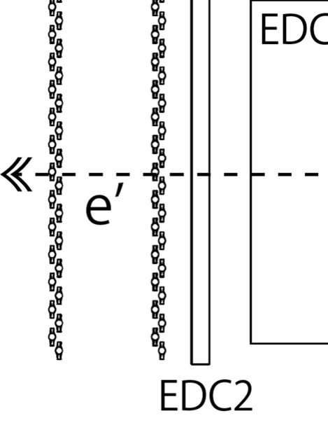
Figure 5: Schematic of the HES detector system. The HES detector system is composed of two drift chambers (EDC1,2) for the particle tracking, and two layers of TOF detectors (ETOF1,2) for the data-taking trigger.

The HES ($e^{\prime}$ spectrometer) detector system consists of two drift chambers (EDC1, EDC2) for the particle tracking, and two layers of TOF detectors (ETOF1, ETOF2) for the data-taking trigger, as shown in Fig. 5. EDC1 is a honeycomb-cell drift chamber with a cell size of 5 mm. EDC1 consists of ten layers with wire configurations of $xx^{\prime}(0^{\circ})uu^{\prime}(-30^{\circ})xx^{\prime}(0^{\circ})vv^{\prime}(+30^{\circ})xx^{\prime}(0^{\circ})$. The typical plane resolution of EDC1 is approximately $\sigma=220$ $\mu$m. The HES-reference plane, on which information of position and angle of particles were used for the momentum analysis in HES, was defined as the mid-plane of EDC1. EDC2 is a planar-drift chamber identical to the KDC. ETOF1 and ETOF2 are plastic scintillation detectors each with a thickness of 10 mm in $z$-direction. The configurations of ETOF1 and ETOF2 are identical. Each ETOF is segmented by 29 in $x$-direction, taking into account a counting rate in each segment. The timing resolution of ETOF was obtained to be $\sigma\simeq 100$ ps in cosmic-ray tests.

III.4 The tilt method in HES

The HES detector system was expected to suffer from huge amount of background electrons which originate from electromagnetic processes. Major sources of background electrons were expected to come from 1) beam electrons which lose their energies via Bremsstrahlung process cite:tsai , and 2) Møller scattering (elastic electron-electron scattering) cite:moller in the target. The reaction cross-sections of these background processes are larger at the smaller scattering angle of $e^{\prime}$. On the other hand, the virtual photon flux, which directly relates to the yield of $\Lambda$ hypernuclei, is also larger at the small $e^{\prime}$ scattering angle, as shown in Fig. 2. Therefore, we attempted to optimize the angular acceptance of HES, taking into account the $S/N$ and yield of $\Lambda$ hypernuclei. For the purpose, we adopted the “tilt method”, which was developed and proven to work sufficiently in the previous $(e,e^{\prime}K^{+})$ experiment (JLab E01-011) cite:miyoshi ; cite:lulin .

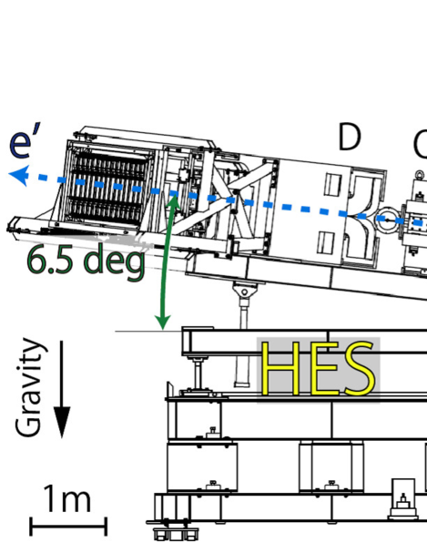
Figure 6: A schematic of the HES side view. HES was vertically tilted to avoid the very small $e^{\prime}$ scattering angle, where the $S/N$ is poor. The tilt angle at 6.5 degrees was chosen by Monte Carlo simulations taking into account both yield and $S/N$.

The tilt method is a method of angular acceptance optimization in which the magnetic spectrometer is tilted vertically, as shown in Fig. 6. A Monte Carlo simulation was performed to optimize the tilt angle. A figure-of-merit (FoM) that was used for the optimization as a reference was defined as follows:

$${\rm FoM}=\frac{R_{{\rm VP}}}{\sqrt{R_{{\rm Brems}}+R_{\textrm{M\o ller}}}},$$ (8)

where $R_{{\rm VP},{\rm Brems},\textrm{M\o ller}}$ are counting rates of electrons associated with the virtual photon, Bremsstrahlung and Møller scattering in HES.

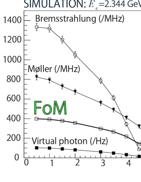
Figure 7: Expected counting rates of electrons associated with the virtual photon ($R_{{\rm VP}}$), Bremsstrahlung ($R_{{\rm Brems}}$) and Møller scattering ($R_{\textrm{M\o ller}}$) in HES by a Monte Carlo simulation. This simulation assumed a 30-$\mu$A electron beam on a 100-mg/cm^{2 12}C target at $E_{e}=2.344$ GeV. A figure of merit (FoM) defined in Eq. (8) is also shown, and the tilt angle was chosen to be 6.5 degrees.

Figure 7 shows the result of the Monte Carlo simulation of a 30-$\mu$A electron beam on a 100-mg/cm^{2 12}C target at $E_{e}=2.344$ GeV. The HES tilt angle was determined to be 6.5 degrees by using this result. The virtual photon flux [Eq. (4)] integrated over the acceptance for scattered electrons (Fig. 9) was evaluated by the Monte Carlo simulation, and was found to be $\Gamma^{int}=(5.67\pm 0.04)\times 10^{-5}$ (/electron) for a momentum range of $p_{e^{\prime}}=0.80$–$0.98$ GeV/$c$.

Table 4 shows typical values of beam intensity $I_{b}$, luminosity $L$, typical angle for scattered electrons $\theta_{e^{\prime}}$, integrated virtual photon flux $\Gamma^{int}$, solid-angle acceptance at the central $K^{+}$ momentum d$\Omega_{K}$, total detection efficiency $\epsilon_{tot}$, counting rates in $e^{\prime}$ spectrometer $R_{e^{\prime}}$, signal yield per hour per 100 nb/sr, $S/N$ for the ground-state doublet peak of ${}^{12}_{\Lambda}$B at the peak position, comparing between E89-009 (without tilt method) cite:miyoshi ; cite:lulin ; cite:miyoshi_dthesis and E05-115 (with tilt method) cite:12LB ; cite:toshi . Because of the tilt method, we were able to increase the luminosity by a factor of 230, while reducing the counting rate in the scattered electron spectrometer by a factor of 1/100. Consequently, although the virtual photon flux is smaller by a factor of 0.14 due to the larger $\theta_{e^{\prime}}$, the yield per a unit time and $S/N$ improved by factors of 60 and 2.5, respectively.

Table 4: Comparison of experimental conditions in E89-009 (without tilt method) and E05-115 (with tilt method).

Experiment	$I_{b}$	$L$	$\theta_{e^{\prime}}$	$\Gamma^{int}$	$d\Omega_{K}$	$\epsilon_{\rm tot}$	$R_{e^{\prime}}$	Yield	$S/N$
(year)	($\mu$A)	(cm-2s-1)	(deg)	(/electron)	(mrad)		(MHz)	per hour
								per 100 nb/sr
E89-009 (2000)	0.6	$4.1\times 10^{33}$	0–4	$4.0\times 10^{-4}$	5.0	0.18	200	0.5	1.1
E05-115 (2009)	35	$9.6\times 10^{35}$	2–13	$5.7\times 10^{-5}$	8.5	0.17	2	30	2.8

III.5 Spectrometer acceptance

The acceptance for each SPL $+$ HKS and SPL $+$ HES optical system was estimated by the Monte Carlo simulation. In the simulation, realistic experimental geometries and magnetic field maps calculated by Opera3D (TOSCA) cite:tosca were used. Figures 8 and 9 show the estimated solid-angle acceptances for SPL $+$ HKS and SPL $+$ HES, respectively. The solid-angle acceptances of SPL $+$ HKS and SPL $+$ HES at each central momentum are approximately 8.5 and 7.0 msr.

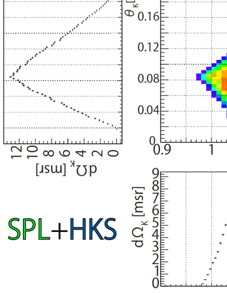
Figure 8: The estimated solid-angle acceptance of SPL $+$ HKS.

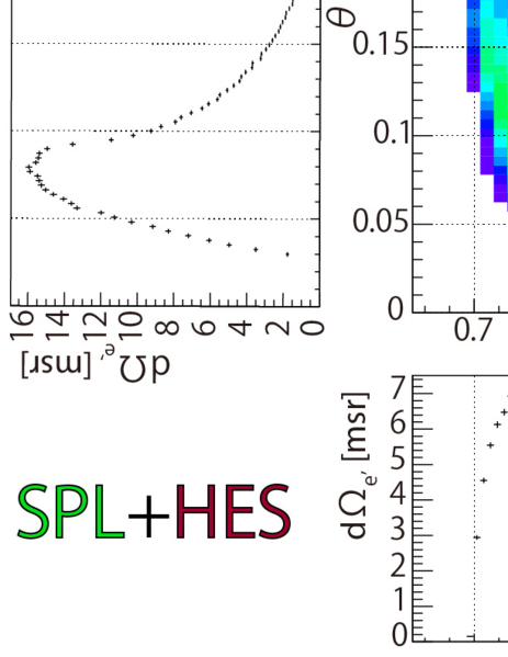
Figure 9: The estimated solid-angle acceptance of SPL $+$ HES.

III.6 Production Target

In the experiment, a natural carbon target and isotopically-enriched solid-targets of ⁷Li, ⁹Be, ¹⁰B, and ⁵²Cr were used for $\Lambda$ hypernuclear production. In addition, we used polyethylene (CH₂) and water (H₂O) targets to measure $\Lambda$ and $\Sigma^{0}$ production from hydrogen nuclei. These targets were used for the energy-scale calibration described in Sec. IV.4. The targets used in the experiment are summarized in Table 5.

Table 5: A list of targets used for the JLab E05-115 experiment.

Target	Reaction	Thickness	Density	Purity	Radiation length	Length in $X_{0}$
		(mm)	(g/cm3)	($\%$)	$X_{0}$ (g/cm2)
CH2	$p$$(e,e^{\prime}K^{+})$$\Lambda$,$\Sigma^{0}$	5.0	0.90	-	44.8	1.0$\times$10-2
	12C$(e,e^{\prime}K^{+})$${}^{12}_{\Lambda}$B
H2O	$p$$(e,e^{\prime}K^{+})$$\Lambda$,$\Sigma^{0}$	5.0	1.00	-	36.1	1.4$\times$10-2
	16O$(e,e^{\prime}K^{+})$${}^{16}_{\Lambda}$N
7Li	7Li$(e,e^{\prime}K^{+})$${}^{7}_{\Lambda}$He	3.9	0.54	99.9	82.8	2.5$\times$10-3
9Be	9Be$(e,e^{\prime}K^{+})$${}^{9}_{\Lambda}$Li	1.0	1.85	100.0	65.2	2.9$\times$10-3
10B	10B$(e,e^{\prime}K^{+})$${}^{10}_{\Lambda}$Be	0.3	2.16	99.9	49.2	1.1$\times$10-3
12C	12C$(e,e^{\prime}K^{+})$${}^{12}_{\Lambda}$B	0.5	1.75	98.89	42.7	2.0$\times$10-3
				(13C:1.11)
52Cr	52Cr$(e,e^{\prime}K^{+})$${}^{52}_{\Lambda}$V	0.2	7.15	99.9	15.3	8.8$\times$10-3

A target holder which had several frames to fix the solid targets was attached to a target ladder as shown in Fig. 10. The target ladder, made primarily of aluminum, was inserted at the SPL entrance with the normal to the target surface at an angle of seventeen degrees with respect to the beam direction, as shown in Fig. 11.

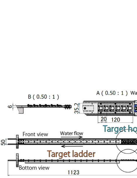
Figure 10: A schematic of the target ladder. The target holder which has some frames to hold targets was put on the ladder. The target holders with different target materials were exchanged two times during the experiment. The dimensions are in mm.

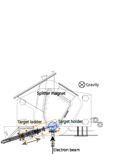
Figure 11: A schematic of the SPL and the target system. The target ladder was inserted at the SPL entrance with the angle of seventeen degrees between the beam direction and the normal of the target surface.

The position of the target holder was controlled by remotely sliding the target ladder in order to change the target intercepting the beam. The target ladder required cooling as the targets were heated by the intense electron beam. For example, the heat deposit was estimated to be approximately 8 W for 50-$\mu$A beam on a 0.1-g/cm² carbon target. Thus, water at the room temperature ($\sim$ 25 ^∘C) continuously flowed along the edge of target ladder to remove the heat from the solid targets. Moreover, the water cell which consisted of 25-$\mu$m Havar foil in back and front was fabricated at the end of target ladder in order to use water as a target. Havar is a non-magnetic cobalt-base alloy which exhibits high strength cite:havar .

Prior to the experiment, the maximum beam current for each target was estimated taking into account the melting point and heat conduction cite:shichijo by using ANSYS cite:ansys , a three-dimensional finite element method software package. As a result, the expected maximum beam currents on the 0.1-g/cm² thick targets were obtained as shown in Table 6. The beam intensities in the experiment were determined according to the above simulation results.

Table 6: The expected maximum beam current for each target with a thickness of 0.1 g/cm² cite:shichijo .

Target	Melting point cite:rika	Expected maximum	Beam current
	(K)	temperature (K)	($\mu$A)
7Li	454	386 (Result without rastering)	30
10B	2349	970	50
12C	4098 (Sublimation point)	521	50
52Cr	2180	988	50

III.7 TUL

For the trigger logic in the experiments, the Tohoku universal logic module (TUL, TUL-8040) cite:yokota , a programmable logic module, was developed to reduce the number of NIM modules and cables needed. A field programmable gate array (FPGA) of ALTERA cite:altera APEX 20K series was mounted on TUL. The major specifications of this module are summarized in Table 7. The introduction of the TUL made it possible to have an on-line grouping trigger as described in Sec. III.8, and it reduced the risks of missed connections among hardware circuits.

Table 7: Major specifications of TUL.

FPGA
Product	ALTERA APEX 20K (EP20K300E)
Maximum gates	728,000
Logic elements	11,520
I/O
Input	NIM: 16 ch
	ECL: 64 ch
Output	NIM: 8 ch
	ECL: 32 ch
Internal clock	33 MHz

III.8 Data-taking trigger

A logical condition of the data-taking trigger for physics run (COIN_trigger) consisted of:

$${\rm COIN}_{{\rm trigger}}={\rm HKS}_{{\rm trigger}}\otimes{\rm HES}_{{\rm trigger}}$$ (9)

where HKS_trigger and HES_trigger are trigger conditions in HKS and HES, respectively, to be explained below.

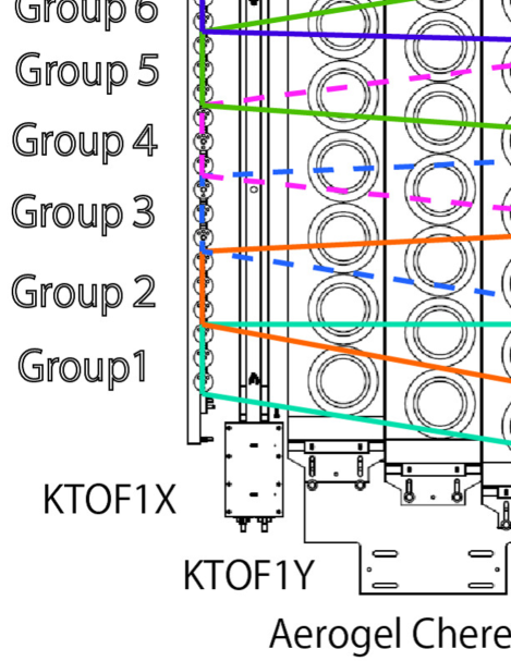
Figure 12: A schematic of the HKS-detector grouping used for the HKS kaon trigger. The HKS detectors were divided into six groups taking into account the optics of HKS.

For the HKS trigger, the detectors were divided into six groups taking into account the HKS optics as shown in Fig. 12. A detector combination for each group was determined by the Monte Carlo simulation in order to minimize the $K^{+}$-overkill ratio as well as background contamination. A trigger was made for each group (HKS${}^{i}_{{\rm trigger}}$) and logically added (OR) to form the HKS trigger (HKS_trigger):

$${\rm HKS}_{{\rm trigger}}=\sum^{6}_{i=1}{\rm HKS}^{i}_{{\rm trigger}},$$ (10)

where $i$ is the group number (grouping trigger). Particles which were not in the HKS optics could be reduced by the grouping trigger. The HKS trigger of the $i^{{\rm th}}$ group consisted of the following logical condition:

$${\rm HKS}^{i}_{{\rm trigger}}={\rm CP}^{i}_{{\rm trigger}}\otimes\overline{{\rm AC}^{i}}\otimes{\rm WC}^{i}$$ (11)

where,

$${\rm CP}^{i}_{{\rm trigger}}={\rm KTOF1X}^{i}\otimes{\rm KTOF1Y}\otimes{\rm KTOF2X}^{i}.$$ (12)

The CP_trigger shown in Sec. III.3 is defined by $\sum^{6}_{i=1}{\rm CP}^{i}_{{\rm trigger}}$. The ACⁱ and WCⁱ in Eq. (11) denote $[$(AC1 $\otimes$ AC2)ⁱ $\oplus$ (AC2 $\otimes$ AC3)ⁱ $\oplus$ (AC3 $\otimes$ AC1)${}^{i}]$, and (WC1 $\otimes$ WC2)ⁱ, respectively. The overline on ACⁱ indicates that the ACⁱ was used as a veto for $\pi^{+}$ suppression. The logic circuit of the HKS trigger is shown in Fig. 13. This complicated trigger condition was realized by the introduction of the TUL (Sec. III.7).

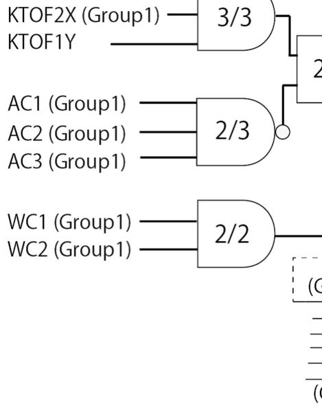
Figure 13: Diagram of logic circuit of the HKS trigger. The HKS detectors were divided into six groups as shown in Fig. 12, taking into account the HKS optics. The trigger was made in each group (HKS${}^{i}_{{\rm trigger}}$), and added logically (OR) being HKS_trigger.

The HES electron trigger was simpler than the HKS kaon trigger. The logic condition of the HES_trigger was as follows:

$${\rm HES}_{{\rm trigger}}={\rm ETOF1}\otimes{\rm ETOF2},$$ (13)

where

$${\rm ETOF1} = \sum^{29}_{j=1}{\rm ETOF1}^{j},$$ (14)

$${\rm ETOF2} = \sum^{29}_{j=1}{\rm ETOF2}^{j}.$$

$$(j:{\rm segment\hskip 2.84544ptnumber})$$

The typical counting rate for each data set is summarized in Table 8. It is noted that the HES-collimator setting for the ⁵²Cr-target data was different from that of the other targets, and thus, HES_trigger and COIN_trigger for the ⁵²Cr target cannot be directly compared to the other targets.

Table 8: Typical trigger rate for each target in the JLab E05-115 experiment.

Target	Beam current	Rate [kHz]
(g/cm2)	($\mu$A)	CPtrigger	HKStrigger	HEStrigger	COINtrigger
CH2 (0.451)	2.0	220	1.8	1200	0.10
H2O (0.500)	2.8	1100	20	1500	1.50
7Li (0.208)	35	540	7.3	2200	0.96
9Be (0.188)	40	710	1.0	2500	1.50
10B (0.056)	40	190	2.0	1600	0.17
12C (0.088)	35	630	7.9	2300	1.30
52Cr (0.134)	8.0	980	11	2500	1.80

IV Analysis

In this section, some of the important analysis steps are described: missing mass reconstruction, $K^{+}$ identification, event selection for $e^{\prime}K^{+}$ coincidence, and energy scale calibration. Background particles which were not in the optics were detected in addition to expected backgrounds of protons and $\pi^{+}$s in the HKS. The origin of the backgrounds and an event selection method which we applied to eliminate them in off-line analysis are discussed in Sec. IV.5.

IV.1 Missing mass reconstruction

The position and angle of a $K^{+}$ and scattered electron at the reference planes in the magnetic spectrometers were measured by the particle detectors. This information was converted to momentum vectors at the target position with backward transfer matrices (BTM) of the optical systems for the SPL $+$ HES and SPL $+$ HKS, respectively, in order to reconstruct a missing mass $M_{{\rm HYP}}$. The $M_{{\rm HYP}}$ is be calculated as follows:

$$M_{{\rm HYP}} = \Bigr{[}E_{{\rm HYP}}^{2}-\vec{p}_{{\rm HYP}}^{\hskip 2.84544pt2}\Bigl{]}^{\frac{1}{2}}$$ (16)

$$= \Bigr{[}(E_{e}+M_{{\rm target}}-E_{K}-E_{e^{\prime}})^{2}$$

$$-(\vec{p}_{e}-\vec{p}_{K}-\vec{p}_{e^{\prime}})^{2}\Bigl{]}^{\frac{1}{2}}$$

$$= \Bigl{[}(E_{e}+M_{{\rm target}}-E_{K}-E_{e^{\prime}})^{2}$$

$$-(p_{e}^{2}+p_{K}^{2}+p_{e^{\prime}}^{2}$$

$$-2p_{e}p_{K}\cos{\theta_{eK}}-2p_{e}p_{e^{\prime}}\cos{\theta_{ee^{\prime}}}$$

$$+2p_{e^{\prime}}p_{K}\cos{\theta_{e^{\prime}K}})\Bigr{]}^{\frac{1}{2}}$$

where $E$, $\vec{p}$ and $M_{{\rm target}}$ are the energy, momentum vectors, and mass of the target nucleus. The beam-momentum vector $\vec{p}_{e}$ was precisely determined by the accelerator ($\Delta E_{e}/E_{e}\leq 10^{-4}$ (FWHM), emittance of 2 $\mu$m$\cdot$mrad). Therefore, only the momentum vectors of $K^{+}$ and scattered electron ($\vec{p}_{K}$ and $\vec{p}_{e^{\prime}}$) are necessary to deduce the missing mass in the experiment. Once $M_{{\rm HYP}}$ is obtained, the $\Lambda$ binding energy $B_{\Lambda}$ can be calculated by:

$$B_{\Lambda}(^{{\rm A}}_{\Lambda}Z)=M(^{{\rm A}-1}Z)+M_{\Lambda}-M_{{\rm HYP}}(^{{\rm A}}_{\Lambda}Z)$$ (17)

where $Z$ denotes the proton number, and $M(^{{\rm A}-1}Z)$ and $M_{\Lambda}$ are the rest masses of a core nucleus at the ground state and a $\Lambda$.

The BTM ($M^{{\rm R2T}}$), which converts the position and angle of a particle at the reference plane to the momentum vector at the target, for each optical system, SPL $+$ HES and SPL $+$ HKS, is written as:

$$\left(\begin{array}[]{c}x_{{\rm T}}\\ x^{\prime}_{{\rm T}}\\ y_{{\rm T}}\\ y^{\prime}_{{\rm T}}\\ p\\ \end{array}\right) = M^{{\rm R2T}}\left(\begin{array}[]{c}x_{{\rm RP}}\\ x^{\prime}_{{\rm RP}}\\ y_{{\rm RP}}\\ y^{\prime}_{{\rm RP}}\\ x_{{\rm RP}}^{2}\\ x_{{\rm RP}}x^{\prime}_{{\rm RP}}\\ \vdots\end{array}\right)$$ (30)

where $x$, $y$, $x^{\prime}$ ($\equiv\frac{p_{x}}{p_{z}}$), $y^{\prime}$ ($\equiv\frac{p_{y}}{p_{z}}$) are the positions and angles at the reference plane (subscript of RP) and the target point (subscript of T), and $p$ is the momentum. For an initial BTM calculation, $x_{{\rm T}}$, $y_{{\rm T}}$ were assumed to be zero as the spatial size of electron beam on the target point was negligibly small (typically $\sigma\simeq 100$ $\mu$m), although the beam was rastered only for low melting-point targets, polyethylene and ⁷Li, as shown in Sec. V.3. The variables, $x^{\prime}_{{\rm T}}$, $y^{\prime}_{{\rm T}}$ and $p$ in Eq. (30) are written as $n^{{\rm th}}$ order polynomial functions as follows:

$$x^{\prime}_{{\rm T}} = \sum^{n}_{a+b+c+d=0}C_{x}(a,b,c,d)(x_{{\rm RP}})^{a}(x^{\prime}_{{\rm RP}})^{b}$$ (31)

$$\times(y_{{\rm RP}})^{c}(y^{\prime}_{{\rm RP}})^{d},$$

$$y^{\prime}_{{\rm T}} = \sum^{n}_{a+b+c+d=0}C_{y}(a,b,c,d)(x_{{\rm RP}})^{a}(x^{\prime}_{{\rm RP}})^{b}$$ (32)

$$\times(y_{{\rm RP}})^{c}(y^{\prime}_{{\rm RP}})^{d},$$

$$p = \sum^{n}_{a+b+c+d=0}C_{p}(a,b,c,d)(x_{{\rm RP}})^{a}(x^{\prime}_{{\rm RP}})^{b}$$ (33)

$$\times(y_{{\rm RP}})^{c}(y^{\prime}_{{\rm RP}})^{d}$$

where $C_{x,y,p}(a,b,c,d)$ are elements of $M^{{\rm R2T}}$.

The initial BTMs were obtained in the full-modeled Monte Carlo simulations. Magnetic field maps, that were used in the Monte Carlo simulation, were calculated by Opera3D (TOSCA). Models of SPL $+$ HKS and SPL $+$ HES were separately prepared, taking into account realistic geometrical information. Then, particles were randomly generated at the target point with uniform distributions over momentum and angular ranges in order to obtain corresponding position and angular information at the reference planes. The initial BTMs were obtained with a fitting algorithm of the singular-value decomposition by inputting the above information at the reference planes and target. The obtained BTMs were not perfect for describing the real optics of our spectrometer systems due to imperfections of the simulation models. In fact, momentum resolutions of $\Delta p/p=10^{-3}$–$10^{-2}$ (FWHM) could be achieved with the initial BTMs, although our goal was $\Delta p/p\simeq 2\times 10^{-4}$ (FWHM). In addition, an energy scale had not been calibrated at this initial stage. Therefore, the initial BTMs needed to be optimized. We optimized the BTMs by a sieve-slit analysis cite:12LB and a semi-automated optimization program as described in Sec. IV.4.

The required computational cost of the optimization process increases as the polynomial order $n$ is increased. For $n=3$, 210 elements [35 (matrix elements) $\times 3$ ($x^{\prime}$, $y^{\prime}$, $p$) elements for HES, and similarly $35\times 3$ elements for HKS] have to be optimized. In contrast, for $n=6$, 1260 elements need to be optimized and their optimizations require much more computation. In the optical simulation, it was found that complexities of $n\geq 6$ are needed for both SPL $+$ HKS and SPL $+$ HES systems to achieve our goal, $\Delta p/p\simeq 2\times 10^{-4}$ FWHM. In the present analysis, therefore, the complexities of $n=6$ were chosen taking also into account the computational cost in the optimization process.

IV.2 $K^{+}$ identification

A $K^{+}$ identification (KID) was essential in both on-line (data-taking trigger; Sec. III.8) and off-line (analysis). Major background particles in HKS were $\pi^{+}$s and protons.

On-line KID was performed with a combination of two types of Cherenkov detectors using radiation media of pure water (refractive index of 1.33) and aerogel (refractive index of 1.05), as shown in Sec. III.8. To avoid over-cutting of $K^{+}$ at the trigger level, the trigger thresholds for water and aerogel Cherenkov detectors were set to be loose, maintaining a DAQ efficiency that was high enough ($>90\%$). Thus, some $\pi^{+}$s and protons remained in data, but were rejected in the off-line analysis.

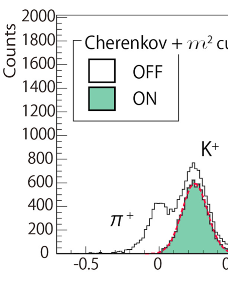
Figure 14: A typical mass squared ($m^{2}$) distribution of data with the 0.451 g/cm² polyethylene target. Colored spectrum shows the $m^{2}$ distribution when event selections of the number of photoelectrons in the aerogel and water Cherenkov detectors were applied as shown in Fig. 15. $K^{+}$s were clearly separated by the event selections by Cherenkov and $m^{2}$ information.

The off-line KID was done by using the number of photoelectrons (NPE) in the Cherenkov detectors, and reconstructed mass squared of the particles. The mass squared ($m^{2}$) was calculated by:

$$m^{2}=p^{2}\Bigl{(}\frac{1}{\beta^{2}}-1\Bigr{)}$$ (34)

where $\beta$ is the velocity factor obtained by TOF and path-length measurements, and $p$ is the particle momentum reconstructed by the BTM as shown in Sec. IV.1. Figure 14 shows a typical mass squared distribution of data with the 0.451 g/cm² polyethylene target.

The top panel of Fig. 15 shows a typical correlation between $m^{2}$ and NPE (sum of three layers) in the aerogel Cherenkov detector. The most probable value of summed NPE for $\pi^{+}$ was at about 30, and those of $K^{+}$ and proton were at about zero. Thus, the $\pi^{+}$s could be separated from $K^{+}$s and protons by applying a cut of NPE as represented by a solid line in Fig. 15.

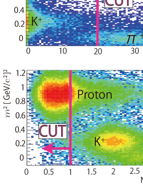
Figure 15: Correlations between the number of photoelectrons (NPE) and $m^{2}$ in AC (sum of three layers) and WC (sum of two layers). $\pi^{+}$s could be separated from $K^{+}$s and protons by a cut of NPE detected by AC, as represented by a solid line in the top panel. Similarly, protons could be distinguished from $\pi^{+}$s and $K^{+}$s by a cut on the normalized NPE detected by the WC, as represented by a solid line in the bottom panel.

We used two types of water Cherenkov detectors (type A cite:taniya and B cite:okayasu_d ) by which detection capabilities of a Cherenkov radiation were different. Main differences between these two types were reflection materials and choice of photo multiplier tubes. The type A was able to detect two times larger NPE than the type B, and the type A was installed for higher momentum side where better capability of proton-$K^{+}$ separation was required cite:gogami . In the analyses, the most probable value of NPE for $K^{+}$ in a layer of the water Cherenkov detector was normalized to unity. A bottom panel of Fig. 15 shows a typical correlation between $m^{2}$ and normalized NPE (sum of two layers) in the water Cherenkov detector. As with the aerogel Cherenkov detector, protons could be separated from $\pi^{+}$s and $K^{+}$s by a cut on the normalized NPE in the water Cherenkov detector, as represented by a solid line in Fig. 15. The colored spectrum in Fig. 14 shows a typical $m^{2}$ distribution with the above cuts of $\pi^{+}$s and protons by the Cherenkov detectors (Fig. 15), and a $m^{2}$ selection of $|m^{2}-m^{2}_{K}|\leq 0.3$ where $m_{K}$ is the known mass of $K^{+}$ cite:pdg . The $K^{+}$ peak in the $m^{2}$ distribution was fitted with a Gaussian function, and the width was found to be $\sigma\simeq(0.29$ GeV/$c^{2})^{2}$. When the off-line KID cuts were selected to maintain a $90\%$ $K^{+}$ survival ratio, the total (on-line and off-line) rejection capabilities of $\pi^{+}$s and protons were $4.7\times 10^{-4}$ and $1.9\times 10^{-4}$, respectively, for the case of a 2-$\mu$A beam on the 0.451 g/cm² polyethylene target cite:gogami .

IV.3 Event Selection for Real $e^{\prime}K^{+}$ Coincidence

In order to find proper coincidences between $e^{\prime}$s and $K^{+}$s in the data, we defined a coincidence time ${\rm T}_{\rm coin}$ as follows:

$${\rm T}_{{\rm coin}}={\rm T}_{{\rm HKS}}-{\rm T}_{{\rm HES}}$$ (35)

where T_HKS and T_HES are reconstructed times at the target position in the HKS and HES, respectively. T_HKS and T_HES were calculated by using the times at the TOF detectors (KTOF, ETOF), the path lengths between the TOF detectors and the target, and the velocity factors ($\beta$) of particles. The path lengths were derived by backward transfer matrices, and the velocity factors were measured by the TOF detectors.

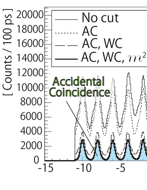
Figure 16: Coincidence time [${\rm T}_{{\rm coin}}$ in Eq. (35)] distribution with and without off-line KID as shown in Sec. IV.2, for the case of a 2-$\mu$A beam on the 0.451-g/cm² polyethylene target. AC, WC and $m^{2}$ denote event selections for $K^{+}$ by the number of photoelectrons in the aerogel and water Cherenkov detectors (Fig. 15), and the reconstructed mass squared, $m^{2}$ (Fig. 14).

Figure 16 shows a typical ${\rm T}_{{\rm coin}}$ distribution with and without the off-line KID as shown in Sec. IV.2. The beam-bunch interval of CEBAF was 2 ns, and the beam-bunch structure was clearly observed with a resolution of $\sigma\simeq 270$ ps. The beam bunch at ${\rm T}_{{\rm coin}}=0$ ns was enhanced after the off-line KID by event selections of the number of photoelectrons in the Cherenkov detectors (AC, WC) and the reconstructed mass squared ($m^{2}$) of particles. Hence, the peak at ${\rm T}_{{\rm coin}}=0$ ns contains events of true coincidence between $e^{\prime}$ and $K^{+}$, while the other peaks contain only accidental coincidence events. In the analyses, events of $|{\rm T}_{{\rm coin}}|\leq 1.0$ ns were selected as the true $e^{\prime}K^{+}$-coincidence events.

IV.4 Energy Scale Calibration

The energy scale calibration was performed by optimizing the BTMs of our magnetic spectrometer systems cite:12LB . For the BTM optimization, we used events of $\Lambda$ and $\Sigma^{0}$ from the 0.451-g/cm² polyethylene target, and those of the ground state of ${}^{12}_{\Lambda}$B from the 0.088-g/cm² natural carbon target. Figure 17 shows the missing mass spectrum from the polyethylene target showing clear peaks of $\Lambda$ and $\Sigma^{0}$ on the top of widely distributed background events. These backgrounds originate from the accidental coincidence and the $\Lambda$/$\Sigma^{0,-}$ production from ¹²C nuclei. The distribution of the accidental background was obtained by selecting events in off-time gates (Sec. IV.3). Moreover, it can also be obtained with a negligibly small statistical uncertainty by the mixed event analysis as applied for analyses of $\Lambda$ hypernuclei cite:7LHe ; cite:12LB ; cite:7LHe_2 . On the other hand, the distribution of $\Lambda$ and $\Sigma^{0,-}$ production from ¹²C nuclei was obtained from the analysis of the natural carbon data.

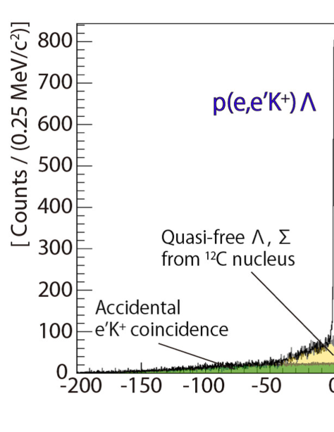
Figure 17: Missing mass spectrum for $\Lambda$ and $\Sigma^{0}$ from the 0.451-g/cm² polyethylene target. There are clear peaks of $\Lambda$ and $\Sigma^{0}$ with the width of about $1.5$-MeV FWHM on the top of background events due to the accidental coincidence and $\Lambda$/$\Sigma^{0,-}$ production from ¹²C nuclei in the polyethylene target. These background distributions were able to be obtained from the real data.

In the BTM-optimization process, a $\chi^{2}$ to be minimized was defined as follows:

$$\chi^{2}=\frac{1}{3}\sum^{3}_{i=1}w_{i}\chi^{2}_{i}$$ (36)

where

$$\chi^{2}_{1} = \frac{1}{N_{\Lambda}}\sum^{N_{\Lambda}}_{j=1}\Bigl{(}\frac{M^{j}_{\Lambda}-M_{\Lambda}}{\sigma_{\Lambda}}\Bigr{)}^{2},$$ (37)

$$\chi^{2}_{2} = \frac{1}{N_{\Sigma^{0}}}\sum^{N_{\Sigma^{0}}}_{k=1}\Bigl{(}\frac{M^{k}_{\Sigma^{0}}-M_{\Sigma^{0}}}{\sigma_{\Sigma^{0}}}\Bigr{)}^{2},$$ (38)

$$\chi^{2}_{3} = \frac{1}{N_{{\rm 12BL}}}\sum^{N_{{\rm 12BL}}}_{l=1}\Bigl{(}\frac{M^{l}_{{\rm 12BL}}-M^{fit}_{{\rm 12BL}}}{\sigma_{{\rm 12BL}}}\Bigr{)}^{2}.$$ (39)

The $M^{j,k,l}_{\Lambda,\Sigma^{0},{\rm 12BL}}$ are the reconstructed missing masses of $\Lambda$, $\Sigma^{0}$ and the ground state of ${}^{12}_{\Lambda}$B. The $M_{\Lambda,\Sigma^{0}}$ are the well known masses of $\Lambda$ and $\Sigma^{0}$ cite:pdg . The $M^{fit}_{{\rm 12BL}}$ denotes a mean value obtained by a single Gaussian fitting to the ground state of ${}^{12}_{\Lambda}$B in an iteration process of the BTM optimization. The $\sigma_{\Lambda,\Sigma^{0},{\rm 12BL}}$ represent expected missing-mass resolutions estimated by the Monte Carlo simulation (Sec. V). The $N_{\Lambda,\Sigma^{0},{\rm 12BL}}$ and $w_{\Lambda,\Sigma^{0},{\rm 12BL}}$ are the number of events and weights for $\Lambda$, $\Sigma^{0}$ and the ground state of ${}^{12}_{\Lambda}$B.

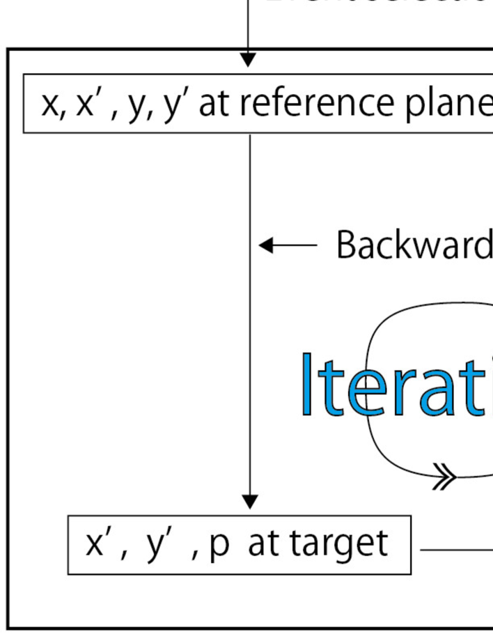
Figure 18: Flow chart of the backward transfer matrix optimization.

Figure 18 shows the flow chart of the BTM optimization. At first, event samples for the tuning were selected with a certain condition. The BTM elements for angles [Eq. (31) and Eq. (32)] and momenta [Eq. (33)] were alternately optimized in the iterative optimization process. We used an weight ratio of $w_{\Lambda}:w_{\Sigma^{0}}:w_{{\rm 12BL}}=1:1:0$ when the angular elements were optimized. The ground-state events of ${}^{12}_{\Lambda}$B were not used in the angular element optimization since kinamatically the angular contributions of the hypernucleus to the missing mass are negligibly small relative to the hyperons (angular contributions for $\Lambda$ are approximately ten times larger than those for ${}^{12}_{\Lambda}$B; Table 10). For the momentum element optimization, on the other hand, the weight ratio of $w_{\Lambda}:w_{\Sigma^{0}}:w_{{\rm 12BL}}=1:1:2$ was used. It is noted that the $M^{fit}_{{\rm 12BL}}$ was not a fixed value, but a mean value of fitting result by a Gaussian-function in each iteration. Thus, in the BTM optimization, the energy scale was calibrated by events of $\Lambda$ and $\Sigma^{0}$, and the ground-state events of ${}^{12}_{\Lambda}$B predominantly contributed to improving the energy resolution. New BMTs used for the next process (loop; Fig. 18) were selected according to checks of missing-mass resolutions and peak positions of $\Lambda$, $\Sigma^{0}$ and the ${}^{12}_{\Lambda}$B-ground state after a number of tuning iterations. Event samples for each next loop were selected with missing masses reconstructed by the new BTMs. The above BTM optimization was repeated until the missing mass resolutions achieved the values expected from simulations. The above process was essentially automated. At some points, however, event-selection conditions were adjusted by hand, depending on the energy resolution, in order to improve $S/N$ of events used for the tuning process.

Systematic errors which originated from the above BTM-optimization process needed to be estimated carefully as the BTM optimization mainly determines the accuracy of the binding energy ($B_{\Lambda}$) and excitation energy ($E_{\Lambda}$) of a $\Lambda$ hypernucleus. In order to estimate the achievable energy accuracy, we performed a full-modeled Monte Carlo simulation with dummy data. The dummy data were generated, taking into account realistic $S/N$ and yields of $\Lambda$, $\Sigma^{0}$ and hypernuclei. Initially the BTMs were perfect in the simulation. Therefore, the BTMs were distorted so as to reproduce broadening and shifts in the missing mass spectra as much as those for the real data. Then, the distorted BTMs were optimized by the exactly same code as that for the real data, and the obtained energies ($B_{\Lambda}$, $E_{\Lambda}$) were compared with assumed energies. The above procedure was tested several times by using different sets of dummy data and BTMs. As a result, it was found that $B_{\Lambda}$ and $E_{\Lambda}$ could be obtained with the accuracy of $<0.09$ MeV and $<0.05$ MeV, respectively using the above calibration method. An uncertainty of target thickness, which was estimated to be $5\%$ according to accuracy of its fabrication and thickness measurement, is considered to be another major contribution to $\Delta B_{\Lambda}$. It is noted that the target thickness uncertainty is canceled out for the $E_{\Lambda}$ calculation. The energy losses of particles in each target were evaluated by the Monte Carlo simulation, and used as a correction to the missing mass calculation as shown in Sec. V.2. The energy loss correction has an uncertainty due to the target thickness uncertainty, and it was evaluated by the Monte Carlo simulation to be taken into account for $\Delta B_{\Lambda}$. Consequently, total systematic errors on $B_{\Lambda}$ and $E_{\Lambda}$ were estimated to be $\pm 0.11$ MeV and $\pm 0.05$ MeV, respectively.

IV.5 $e^{-}e^{+}$ background in HKS

Electromagnetic background particles such as electrons from the Bremsstrahlung or Møller scattering were expected in the HES. These were drastically reduced by the tilt method as shown in Sec. III.4. However, in the HKS, background events which are attributed to $e^{-}e^{+}$ pair production were detected in addition to the expected background hadrons ($\pi^{+}$ and proton). Figure 19 shows a typical distribution of $x$ versus $x^{\prime}$ at the reference plane for the case of ⁷Li target. Plots in a solid box indicate particles within the HKS optics. Apart from the solid box, however, there are events constituting a band structure in the dashed-line box.

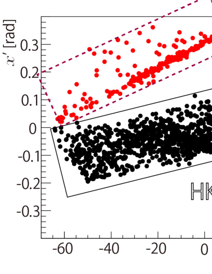
Figure 19: Distribution of $x$ versus $x^{\prime}$ at the HKS reference plane in the case of the ⁷Li target. Events in a solid box were in the HKS optics. However, there were events which were not on the optics as shown in a dashed-line box.

The events were traced back toward upstream direction by using the particle-tracking information as shown in Fig. 20, and it was found that they came from secondary scattering at the low-momentum side of vacuum-extension box which was made of a stainless steel SUS304.

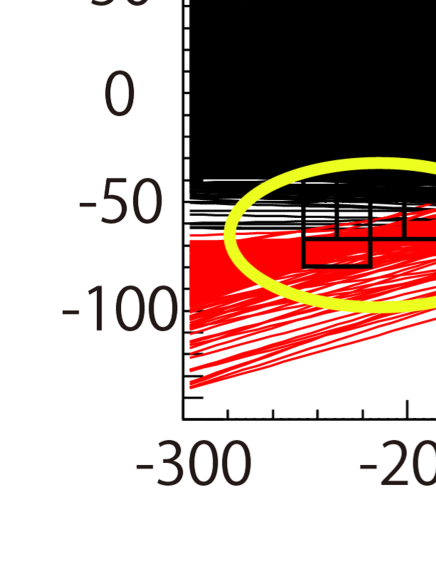
Figure 20: Reconstructed HKS tracks on the $xz$-plane in the case of ⁷Li target for the real data. There were particles coming from the lower momentum side ($x<0$) of the vacuum-extension box which was made of a stainless steel SUS304. As a result of the Monte Carlo simulation, the source of these backgrounds is considered to be positrons generated in the target. The positrons with certain momentum and scattering angle would hit the vacuum-extension box. It would result in a detection of positrons and electrons which are generated via the pair creation process in the walls of the vacuum-extension box.

The Monte Carlo simulation reproduced such a situation. Positrons hit the vacuum-extension box when the positrons with the momenta of $p=0.8$–1.0 GeV/$c$ and the scattered angle of $\theta=0$–2 mrad were generated in the target via the e^-e⁺-pair production process. Then, more positrons and electrons were generated in the vacuum-extension box, and they were detected in HKS. These background events were eliminated in the off-line analysis by selecting events on the $x$ versus $x^{\prime}$ histogram as shown in Fig. 19.

These background events were recognized during the experiment. However, it seemed to be hard to shield them physically since they passed through inside of the vacuum-extension box according to the on-line analysis as shown in Fig. 20. Moreover, physical shields could be another source of background events. Therefore, we decided to take data with these background particles in the experiment. The counting rate of the background for each target was normalized by the areal density of the target and beam intensity. As a result, it was found that the background rate increased with a square of the target-proton number $Z^{2}$. It indicates that this background originated from an electro-magnetic process. This is a major reason why we used the lower beam-intensity on the ⁵²Cr target compared to the other lighter targets.

The experimental setup of the future hypernuclear experiment E12-15-008, which will be carried out with HKS and HRS cite:hrs in JLab Hall A, is being optimized to avoid the above background events cite:pac44 .

V Missig-mass resolution achieved

Major factors which contribute to the missing-mass resolution are presented in this section. The missing-mass resolution cannot be easily estimated by considering each contribution separately as they are not independent from each other. Therefore, a full-modeled Monte Carlo simulation was performed to investigate the achievable resolution taking into account all of the major factors. A comparison between the expected mass resolutions and those of final results for typical hypernuclei is shown in Sec. V.4.

The contributions to the missing-mass resolution are dominated by the following sources: 1) the intrinsic mass-resolution due to momentum and angular resolutions of spectrometers (Sec. V.1), 2) mass-offset effect due to energy-loss variations in the finite volumes of the targets (Sec. V.2), and 3) production point displacements from the assumed origin of the BTMs (Sec. V.3). Momentum straggling in the target also contributes to the mass-resolution, and was estimated to be less than 50 and 150-keV FWHM for production of hypernuclei and $\Lambda$, respectively, when they are produced at the target center. However, it is worth noting that the energy-straggling contribution is somewhat smaller than from the above three major factors.

V.1 Intrinsic mass resolution

The intrinsic mass resolution, which is a kinematical broadening due to the momentum and angular resolutions of the magnetic spectrometers as well as beam qualities such as a beam-energy spread, was estimated by the Monte Carlo simulation. A typical value of the beam-energy spread was $\Delta E/E=3.0\times 10^{-5}$ which was used for the simulation. On the other hand, the spectrometers’ resolutions for the momentum and angle at the target point were evaluated, as shown in Table 9, taking into account achieved resolutions of the position and angle measurements at the reference planes from the particle detectors.

Table 9: Resolutions for the reconstructed momentum and angle in the optical systems of SPL $+$ HKS and SPL $+$ HES obtained by the Monte Carlo simulation taking into account the achieved position and angular resolutions of the particle detectors.

Spectrometer	SPL$+$HES	SPL$+$HKS
Particle	$e^{\prime}$	$K^{+}$
$\Delta p$/$p$	4.2$\times 10^{-4}$	2.0$\times 10^{-4}$
$\Delta\theta$ (RMS) (mrad)	4.0	0.4

When the kinematical variables $p_{e,e^{\prime},K}$ and $\theta_{ee^{\prime},eK,e^{\prime}K}$ are varied by $\Delta p_{e,e^{\prime},K}$ and $\Delta\theta_{ee^{\prime},eK,e^{\prime}K}$, the variations of $M_{{\rm HYP}}$ can be calculated as follows:

$$\frac{\partial M_{{\rm HYP}}}{\partial p_{e}}\Delta p_{e} = +\frac{1}{M_{{\rm HYP}}}\Bigl{[}\beta_{e}(M_{{\rm target}}-E_{K}-E_{e^{\prime}})$$ (40)

$$+p_{e^{\prime}}\cos{\theta_{ee^{\prime}}}+p_{K}\cos{\theta_{eK}}\Bigr{]}\Delta p_{e},$$

$$\frac{\partial M_{{\rm HYP}}}{\partial p_{e^{\prime}}}\Delta p_{e^{\prime}} = -\frac{1}{M_{{\rm HYP}}}\Bigl{[}\beta_{e^{\prime}}(M_{{\rm target}}+E_{e}-E_{K})$$ (41)

$$-p_{e}\cos{\theta_{ee^{\prime}}}+p_{K}\cos{\theta_{e^{\prime}K}}\Bigr{]}\Delta p_{e^{\prime}},$$

$$\frac{\partial M_{{\rm HYP}}}{\partial p_{K}}\Delta p_{K} = -\frac{1}{M_{{\rm HYP}}}\Bigl{[}\beta_{K}(M_{{\rm target}}+E_{e}-E_{e^{\prime}})$$ (42)

$$-p_{e}\cos{\theta_{eK}}+p_{e^{\prime}}\cos{\theta_{e^{\prime}K}}\Bigr{]}\Delta p_{K},$$

$$\frac{\partial M_{{\rm HYP}}}{\partial\theta_{ee^{\prime}}}\Delta\theta_{ee^{\prime}} = -\Bigl{(}\frac{1}{M_{{\rm HYP}}}p_{e}p_{e^{\prime}}\sin{\theta_{ee^{\prime}}}\Bigr{)}\Delta\theta_{ee^{\prime}},$$ (43)

$$\frac{\partial M_{{\rm HYP}}}{\partial\theta_{eK}}\Delta\theta_{eK} = -\Bigl{(}\frac{1}{M_{{\rm HYP}}}p_{e}p_{K}\sin{\theta_{eK}}\Bigr{)}\Delta\theta_{eK},$$ (44)

$$\frac{\partial M_{{\rm HYP}}}{\partial\theta_{e^{\prime}K}}\Delta\theta_{e^{\prime}K} = +\Bigl{(}\frac{1}{M_{{\rm HYP}}}p_{e^{\prime}}p_{K}\sin{\theta_{e^{\prime}K}}\Bigr{)}\Delta\theta_{e^{\prime}K}.$$ (45)

The above partial differentiations were calculated event by event in the Monte Carlo simulation and their mean values for the typical reactions $p$$(e,e^{\prime}K^{+})$$\Lambda$, ⁷Li$(e,e^{\prime}K^{+})$${}^{7}_{\Lambda}$He, and ¹²C$(e,e^{\prime}K^{+})$${}^{12}_{\Lambda}$B are summarized in Table 10.

Table 10: Mean values of the partial differentiations in Eqs. (40–45) obtained in the Monte Carlo simulation. Intrinsic mass resolution $\Delta M^{{\rm int}}_{{\rm HYP}}$ which is defined by Eq. (V.1) is shown for each target in the last row.

	$\Lambda$	${}^{7}_{\Lambda}$He	${}^{12}_{\Lambda}$B
Assumed $B_{\Lambda}$ (MeV)	-	5.5	11.37
$\frac{\partial M_{{\rm HYP}}}{\partial p_{e}}$ $\Bigl{(}\frac{{\rm keV/}c^{2}}{{\rm MeV/}c}\Bigr{)}$	742	957	974
$\frac{\partial M_{{\rm HYP}}}{\partial p_{e^{\prime}}}$ $\Bigl{(}\frac{{\rm keV/}c^{2}}{{\rm MeV/}c}\Bigr{)}$	$-$747	$-$958	$-$975
$\frac{\partial M_{{\rm HYP}}}{\partial p_{K}}$ $\Bigl{(}\frac{{\rm keV/}c^{2}}{{\rm MeV/}c}\Bigr{)}$	$-$673	$-$885	$-$902
$\frac{\partial M_{{\rm HYP}}}{\partial\theta_{ee^{\prime}}}$ $\Bigl{(}\frac{{\rm keV/}c^{2}}{{\rm mrad}}\Bigr{)}$	$-$124	$-$21	$-$13
$\frac{\partial M_{{\rm HYP}}}{\partial\theta_{eK}}$ $\Bigl{(}\frac{{\rm keV/}c^{2}}{{\rm mrad}}\Bigr{)}$	$-$258	$-$51	$-$30
$\frac{\partial M_{{\rm HYP}}}{\partial\theta_{e^{\prime}K}}$ $\Bigl{(}\frac{{\rm keV/}c^{2}}{{\rm mrad}}\Bigr{)}$	109	20	12
$\Delta M^{{\rm int}}_{{\rm HYP}}$ (keV/$c^{2}$) (FWHM)	733	414	410

If all of the variables are assumed to be independent from each other, the intrinsic missing-mass resolution $\Delta M^{{\rm int}}_{{\rm HYP}}$ is obtained to be:

$$(\Delta M^{{\rm int}}_{{\rm HYP}})^{2} = \Bigl{(}\frac{\partial M_{{\rm HYP}}}{\partial p_{e}}\Delta p_{e}\Bigr{)}^{2}+\Bigl{(}\frac{\partial M_{{\rm HYP}}}{\partial p_{e^{\prime}}}\Delta p_{e^{\prime}}\Bigr{)}^{2}$$

$$+\Bigl{(}\frac{\partial M_{{\rm HYP}}}{\partial p_{K}}\Delta p_{K}\Bigr{)}^{2}+\Bigl{(}\frac{\partial M_{{\rm HYP}}}{\partial\theta_{ee^{\prime}}}\Delta\theta_{ee^{\prime}}\Bigr{)}^{2}$$

$$+\Bigl{(}\frac{\partial M_{{\rm HYP}}}{\partial\theta_{eK}}\Delta\theta_{eK}\Bigr{)}^{2}+\Bigl{(}\frac{\partial M_{{\rm HYP}}}{\partial\theta_{e^{\prime}K}}\Delta\theta_{e^{\prime}K}\Bigr{)}^{2},$$

The calculated results of $\Delta M^{{\rm int}}_{{\rm HYP}}$ for the typical targets by using the momentum and angular resolutions shown in Table 9 are shown in the last row of Table 10. It should be emphasized that $\Delta M^{{\rm int}}_{{\rm HYP}}$ is just a reference value to be compared with other effects on the mass resolution because the variables in Eq. (V.1) are not independent from each other.

V.2 Mass offset due to the energy loss in target

The momentum of the beam $p^{{\rm det}}_{e}$ is precisely determined by the accelerator. However, the beam momentum at the production point $p_{e}$ is lower because of momentum loss in the target. For $e^{\prime}$ and $K^{+}$, on the other hand, the momenta at the production point $p_{e^{\prime},K}$ are higher than those measured by the spectrometers $p^{{\rm mea}}_{e^{\prime},K}$. Therefore,

$$p^{{\rm det}}_{e} = p_{e}+\delta p_{e}$$ (47)

$$p^{{\rm mea}}_{e^{\prime}} = p_{e^{\prime}}-\delta p_{e^{\prime}}$$ (48)

$$p^{{\rm mea}}_{K} = p_{K}-\delta p_{K}$$ (49)

where $\delta p_{e,e^{\prime},K}$ are the momentum losses in the target. The correction for the momentum loss was applied to the missing mass derivation as follows:

$$p_{e} = p^{{\rm det}}_{e}-\delta p_{e}^{{\rm center}}$$ (50)

$$p_{e^{\prime}} = p^{{\rm mea}}_{e^{\prime}}+\delta p_{e^{\prime}}^{{\rm center}}$$ (51)

$$p_{K} = p^{{\rm mea}}_{K}+\delta p_{K}^{{\rm center}}$$ (52)

where $\delta p_{e,e^{\prime},K^{+}}^{{\rm center}}$ are the correction factors which were obtained in the Monte Carlo simulation assuming hypernuclei or hyperons produced at the target center. However, this correction cannot compensate for the momentum loss properly when the production point is displaced from the center particularly along $z$-direction, and thus it caused missing mass broadening. Assuming $\delta p^{{\rm center}}=\delta p_{e}^{{\rm center}}=\delta p_{e^{\prime}}^{{\rm center}}=\delta p_{K}^{{\rm center}}$ and that the angular contribution due to the multiple scattering is small, the missing mass shift between production points of front and back surfaces of the target $\Delta M^{{\rm eloss}}_{{\rm HYP}}$ can be estimated as follows:

$$\Delta M^{{\rm eloss}}_{{\rm HYP}} \simeq -\frac{\partial M_{{\rm HYP}}}{\partial p_{e}}(2\delta p_{e}^{{\rm center}})$$

$$-\Bigl{[}\frac{\partial M_{{\rm HYP}}}{\partial p_{e^{\prime}}}(2\delta p_{e^{\prime}}^{{\rm center}})+\frac{\partial M_{{\rm HYP}}}{\partial p_{K}}(2\delta p_{K}^{{\rm center}})\Bigr{]}$$

$$= -2\delta p^{{\rm center}}\Bigl{(}\frac{\partial M_{{\rm HYP}}}{\partial p_{e}}+\frac{\partial M_{{\rm HYP}}}{\partial p_{e^{\prime}}}+\frac{\partial M_{{\rm HYP}}}{\partial p_{K}}\Bigr{)}.$$

The $\Delta M^{{\rm eloss}}_{{\rm HYP}}$ was calculated taking into account the momentum loss for each particle, and found to be $\pm 0.31$, $\pm 0.20$, and $\pm 0.06$ MeV/$c^{2}$ for the polyethylene, ⁷Li and ¹²C targets, respectively.

V.3 Production point displacement from an assumed origin of BTM

The BTMs were generated with an assumption that hypernuclei are produced at the point of the target center. In the actual situation, however, the production points could be displaced from the assumed origin along with the $z$-direction. In addition, for the polyethylene and ⁷Li targets, the beam rastering in the $x$ and $y$ directions was applied in order to avoid melting of the targets from beam heating. Figures 21 and 22 show the raster patterns for the polyethylene and ⁷Li targets for the actual data. The raster patterns were obtained by measuring on an event by event basis the voltages applied to the dipole magnets used for rastering. The displacement of the production point from the assumed BTM origin affects the missing mass resolution. It is noted that a counting rate around $0.05<y<0.05$ cm for the polyethylene target is low because the target was cracked due to heat despite the rastering. During the experiment, the polyethylene target was moved to new position every a few hours. The raster pattern and trigger rates were monitored in order to avoid serious damage on the target.

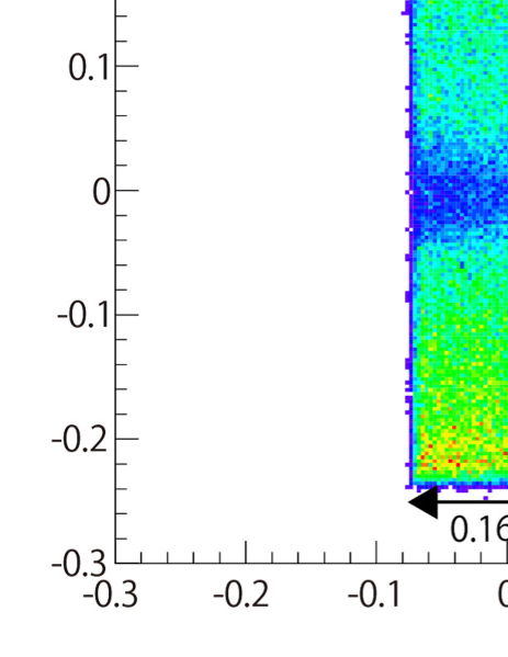
Figure 21: Beam profile on the polyethylene target. The beam was rastered in the area of $0.16^{x}\times 0.46^{y}$ cm² for the polyethylene target.

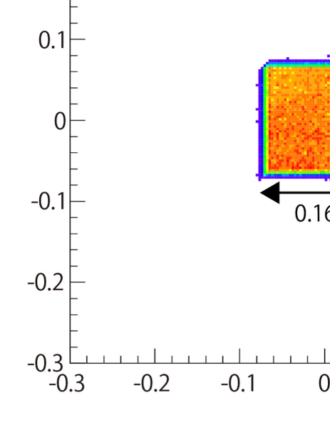
Figure 22: Beam profile on the ⁷Li target. The Beam was rastered in the area of $0.16^{x}\times 0.16^{y}$ cm² for the ⁷Li target.

V.3.1 $z$-dependence

The target has a finite thickness, and thus, points where $\Lambda$ hypernuclei or hyperons are produced are varied event by event in the target along with the beam direction ($z$ direction). We performed a Monte Carlo simulation to study an effect on the missing mass due to the $z$ displacement from the BTM origin. In the simulation, no target was placed and particles ($e$, $e^{\prime}$ and $K^{+}$) were randomly generated in the range of actual target thickness along with the $z$-direction. As a result, the $z$ displacement was found to yield the missing-mass shift. The missing-mass broadening $\Delta M^{{\rm Matrix}(z)}_{{\rm offset}}$ due to the mass shifts for the production of $\Lambda$, ${}^{7}_{\Lambda}$He and ${}^{12}_{\Lambda}$B were found to be $\pm 0.37$, $\pm 0.34$, and $\pm 0.09$ MeV/$c^{2}$, respectively.

V.3.2 $x$ and $y$-dependence

The beam was rastered for the polyethylene and ⁷Li targets because their melting points were lower than the other targets. The raster areas were $0.16^{x}\times 0.46^{y}$ cm² and $0.16^{x}\times 0.16^{y}$ cm² for these two targets. (See Figs. 21 and 22) Therefore, production points can be displaced from the BTM origin in the $x$ and $y$ directions for these targets. To investigate effects on the missing mass due to the displacements in $x$ and $y$ directions, Monte Carlo simulations were performed as was done for the $z$ displacement. The mass broadening due to the $x$ and $y$ displacements was found to be less than a few hundred keV. However, this effect can be removed because we measured a correlation of $x$ and $y$ positions versus the missing mass for $\Lambda$ in the data analysis. The obtained correlation was used for corrections of the $x$ and $y$ displacements for the production of $\Lambda$ ($\Sigma^{0}$) and ${}^{7}_{\Lambda}$He.

V.4 Comparison between the full estimation and obtained results

The missing-mass resolution cannot be simply estimated by each contribution from the above sources because some of them are not independent from each other. In addition, the missing-mass resolution depends on achieved momentum and angular resolutions after the BTM optimization (energy scale calibration, Sec. IV.4). Therefore, we performed a full modeled Monte Carlo simulation to estimate the realistic missing-mass resolution. In the simulation, the calibration analyses that were used for the real data were applied to various sets of dummy data and distorted BTMs as described in Sec. IV.4. Typical results obtained in the simulation and the results of the real data analyses cite:7LHe_2 ; cite:12LB are tabulated in Table 11, and these are fairly consistent. Figure 23 shows the obtained $B_{\Lambda}$ spectrum for ${}^{12}_{\Lambda}$B cite:12LB with the energy resolution of 0.54-MeV FWHM.

Table 11: A comparison of missing mass resolution between the Monte Carlo simulation and real data analyses for production of $\Lambda$, ${}^{7}_{\Lambda}$He, and ${}^{12}_{\Lambda}$B in JLab E05-115.

Hyperon/Hypernucleus		$\Lambda$	${}^{7}_{\Lambda}$He	${}^{12}_{\Lambda}$B
Target		CH2	7Li	12C
Thickness $($g/cm${}^{2})$		0.451	0.208	0.088
Length in $z$ $($mm$)$		5.0	3.9	0.5
$\Delta M^{{\rm int}}_{{\rm HYP}}$ FWHM (MeV/$c^{2}$)		0.73	0.41	0.41
$\Delta M^{{\rm Matrix}(z)}_{{\rm offset}}$ (MeV/$c^{2}$)		$\pm 0.37$	$\pm 0.34$	$\pm 0.09$
$\Delta M^{{\rm eloss}}_{{\rm offset}}$ (MeV/$c^{2}$)		$\pm 0.31$	$\pm 0.20$	$\pm 0.06$
$\Delta M$	Simulation	1.6	1.3	0.5
FWHM	Real data	1.5	1.3 cite:7LHe_2	0.54 cite:12LB
(MeV/$c^{2}$)		(Fig. 17)		(Fig. 23)

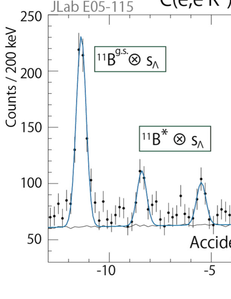
Figure 23: A binding energy spectrum for the ¹²C$(e,e^{\prime}K^{+})$${}^{12}_{\Lambda}$B reaction using a natural carbon target with a thickness of 0.088 g/cm² in JLab E05-115. Peak structures which correspond to (¹¹B${}^{g.s.}\otimes s_{\Lambda}$), (¹¹B${}^{*}\otimes s_{\Lambda}$), and (¹¹B${}^{g.s.}\otimes p_{\Lambda}$) clearly can be seen with a FWHM of 0.54 MeV (refer to Ref. cite:12LB ).

VI Conclusion

We study one of the fundamental forces, the strong force, by investigating the $\Lambda N$ interaction through spectroscopy of $\Lambda$ hypernuclei. $\Lambda$-hypernuclear spectroscopy with the $(e,e^{\prime}K^{+})$ reaction, which complements experiments with other reactions, was established in JLab. The unique features of the $(e,e^{\prime}K^{+})$ experiment are the higher energy resolution ($\Delta E\simeq 0.5$-MeV FWHM) and better accuracy of the $\Lambda$ binding energy ($\Delta B_{\Lambda}\leq 0.2$ MeV) compared to existing reaction spectroscopy with the $(K^{-},\pi^{-})$ and $(\pi^{+},K^{+})$ reactions, thanks to the primary electron beam at JLab.

A new spectrometer system consisting of the SPL $+$ HES $+$ HKS was designed to measure hypernuclei up to the medium heavy mass region ($A\leq 52$) in the latest hypernuclear experiment E05-115 at JLab Hall C. In addition, we developed novel techniques of semi-automated energy scale calibration using $\Lambda$ and $\Sigma^{0}$ production from the hydrogen target. The new spectrometer system and calibration technique resulted in the best energy resolution and $B_{\Lambda}$ accuracy (e.g. FWHM $=0.54$ MeV and $\Delta B^{sys.}_{\Lambda}=0.11$ MeV for ¹²C$(e,e^{\prime}K^{+})$${}^{12}_{\Lambda}$B) in reaction spectroscopy of $\Lambda$ hypernuclei, and spectroscopic results for ${}^{7}_{\Lambda}$He cite:7LHe_2 , ${}^{10}_{\Lambda}$Be cite:10LBe , and ${}^{12}_{\Lambda}$B cite:12LB have been successfully obtained and published. For the ⁵²Cr target, on the other hand, $e^{-}e^{+}$ background events which increased in proportion to a square of target proton number $Z^{2}$ caused high rates and high multiplicity in the HKS detector system. The analysis for the ⁵²Cr$(e,e^{\prime}K^{+})$${}^{52}_{\Lambda}$V is in progress under such a severe multiplicity condition.

The established techniques particularly energy calibration method will be a basis and be further developed in the next hypernuclear experiments at JLab cite:pac44 ; cite:pac45 ; cite:loi208 .

References

- (1) O. Hashimoto and H. Tamura, Progress in Particle and Nuclear Physics 57, 564653 (2006).
- (2) A. Feliciello and T. Nagae, Reports on Progress in Physics 78, 096301 (2015).
- (3) A. Gal, E.V. Hungerford, and D.J. Millener, Rev. Mod. Phys. 88, 035004 (2016).
- (4) H. Sugimura et al. (J-PARC E10 Collaboration), Physics Letters B 729, 39–44, (2014).
- (5) T.O. Yamamoto et al. (J-PARC E13 Collaboration), Phys. Rev. Lett. 115, 222501 (2015).
- (6) R. Honda et al. (J-PARC E10 Collaboration), Phys. Rev. C 96, 014005 (2017).
- (7) T.R. Saito et al., Nucl. Phys. A 881, 218–227 (2012).
- (8) C. Rappold et al. (HypHI Collaboration), Phys. Rev. C 88, 041001(R) (2013).
- (9) C. Rappold et al., Nucl. Phys. A 913, 170–184 (2013); Phys. Lett. B 747, 129–134 (2015).
- (10) Y. Zhu (STAR Collaboration), Nucl. Phys. A 904–905, 551c–554c (2013).
- (11) J. Adam et al. (ALICE Collaboration), Phys. Lett. B 754, 360 (2016).
- (12) A. Esser, S. Nagao, F. Schulz, P. Achenbach et al. (A1 Collaboration), Phys. Rev. Lett. 114, 232501 (2015).
- (13) F. Schulz, P. Achenbach et al. (A1 Collaboration), Nucl. Phys. A 954, 149 (2016).
- (14) P. Achenbach et al., JPS Conf. Proc. 17, 011001 (2017).
- (15) S.N. Nakamura, A. Matsumura. Y. Okayasu, T. Seva, V. M. Rodriguez, P. Baturin, L. Yuan et al. (HKS (JLab E01-011) Collaboration), Phys. Rev. Lett. 110, 012502 (2013).
- (16) L. Tang, C. Chen, T. Gogami, D. Kawama, Y. Han et al. (HKS (JLab E05-115 and E01-011) Collaborations), Phys. Rev. C 90, 034320 (2014).
- (17) T. Gogami, C. Chen, D. Kawama et al. (HKS (JLab E05-115) Collaboration), Phys. Rev. C 93, 034314 (2016).
- (18) T. Gogami, C. Chen, D. Kawama et al. (HKS (JLab E05-115) Collaboration), Phys. Rev. C 94, 021302(R) (2016).
- (19) M. Danysz and J. Pniewski, Phil. Mag. 44 (1953).
- (20) M. Juri et al., Nucl. Phys. B 52, 1 (1973).
- (21) T. Hasegawa et al., Phys. Rev. C 53, 1210 (1996).
- (22) H. Hotchi et al., Phys. Rev. C 64, 044302 (2001).
- (23) P. Dluzewski et al., Nucl. Phys. A 484, 520 (1988).
- (24) D.H. Davis, Nucl. Phys. A 754, 3c–13c (2005).
- (25) E. Botta, T. Bressani, A. Feliciello, Nucl. Phys. A 960, 165–179 (2017).
- (26) T. Motoba, M. Sotona, and K. Itonaga, Prog. Theor. Phys. Suppl. 117, 123 (1994).
- (27) H. Tamura et al., Phys. Rev. Lett. 84, 5963 (2000).
- (28) K. Tanida et al., Phys. Rev. Lett. 86, 1982 (2001).
- (29) H. Akikawa et al., Phys. Rev. Lett. 88, 082501 (2002).
- (30) M. Ukai et al., Phys. Rev. Lett. 93, 232501 (2004); Phys. Rev. C 73, 012501(R) (2006); Phys. Rev. C 77, 054315 (2008).
- (31) K. Hosomi et al., Prog. Theor. Exp. Phys., 081D01 (2015).
- (32) S.B. Yang et al., JPS Conf. Proc. 17, 012004 (2017); H. Tamura et al., JPS Conf. Proc. 17, 011004 (2017).
- (33) K.A. Olive et al. (Particle Data Group), Chin. Phys. C 38, 090001 (2014) and 2015 update.
- (34) A. Gal, Phys. Lett. B 744, 352–357 (2015).
- (35) D. Gazda and A. Gal, Phys. Rev. Lett. 116, 122501 (2016); Nucl. Phys. A 954, 161 (2016).
- (36) Y. Yamamoto, T. Furumoto, N. Yasutake, and Th.A. Rijken, Phys. Rev. C 90, 045805 (2014).
- (37) M. Isaka, K. Fukukawa, M. Kimura, E. Hiyama, H. Sagawa, and Y. Yamamoto, Phys. Rev. C 89, 024310 (2014).
- (38) M.T. Win and K. Hagino, Phys. Rev. C 78, 054311 (2008).
- (39) B.N. Lu, E. Hiyama, H. Sagawa, and S. G. Zhou, Phys. Rev. C 89, 044307 (2014).
- (40) W.X. Xue, J.M. Yao, K. Hagino, Z.P. Li, H. Mei, and Y. Tanimura, Phys. Rev. C 91, 024327 (2015).
- (41) E. Hiyama, Y. Yamamoto, T. Motoba, M. Kamimura, Phys. Rev. C 80, 054321 (2009).
- (42) E. Hiyama and Y. Yamamoto, Prog. Theor. Phys. 128, 1 (2012).
- (43) P. Bydovsk, M. Sotona, T. Motoba, K. Itonaga, K. Ogawa, and O. Hashimoto, Nucl. Phys. A 881, 199 (2012).
- (44) Master’s Theses, Tohoku University, Sendai, Japan (all in Japanese): J. Kusaka, “Design of an experiment for electro-production spectroscopy of medium-heavy hypernuclei”, 2014; M. Fujita, “Design of an experiment for Lambda hypernuclear reaction spectroscopy in wide mass range by the reaction”, 2016.
- (45) O. Benhar, F. Garibaldi, T. Gogami, E.C. Markowitz, S.N. Nakamura, J. Reinhold, L. Tang, G.M. Urciuoli, I. Vidana, Letter of Intend to JLab PAC45, LOI12-17-003, “Studying interactions in nuclear matter with the 208PbTl reaction”, 2017.
- (46) T. Gogami, Doctoral Thesis, “Spectroscopic research of hypernuclei up to medium-heavy mass region with the reaction”, Tohoku University, Sendai, Japan, 2014.
- (47) T. Miyoshi et al. (HNSS Collaboration), Phys. Rev. Lett. 90, 232502 (2003).
- (48) L. Yuan et al. (HNSS Collaboration), Phys. Rev. C 73, 044607 (2006).
- (49) O. Hashimoto et al., Nucl. Phys. A 835, 121–128 (2010).
- (50) S.N. Nakamura, T. Gogami, and L. Tang, JPS Conf. Proc. 17, 011002 (2017).
- (51) G.M. Urciuoli et al. (Jefferson Lab Hall A Collaboration), Phys. Rev. C 91, 034308 (2015).
- (52) M. Iodice et al. (Jefferson Lab Hall A Collaboration), Phys. Rev. Lett. 99, 052501 (2007).
- (53) F. Cusanno et al. (Jefferson Lab Hall A Collaboration), Phys. Rev. Lett. 103, 202501 (2009).
- (54) M. Sotona and S. Frullani, Prog. Theor. Phys. Suppl. 177, 151 (1994).
- (55) E.V. Hungerford, Prog. Theor. Phys. Suppl. 117, 135 (1994).
- (56) G. Xu and E.V. Hungerford, Nucl. Instrum. Methods Phys. Res. Sect. A 501, 602–614 (2003).
- (57) R. Bradford et al., Phys. Rev. C 73, 035202 (2006).
- (58) T. Gogami et al., Nucl. Instrum. Methods Phys. Res. Sect. A 729, 816–824 (2013).
- (59) Y. Fujii et al., Nucl. Instrum. Methods Phys. Res. Sect. A 795, 351–363 (2015).
- (60) Y. Tsai, Rev. Mod. Phys. 46, 4 (1974).
- (61) C. Itzykson, J. Zuber, Quantum Field Theory (Dover, 1980).
- (62) T. Miyoshi, Doctoral Thesis, “Spectroscopic study of hypernuclei by the reaction”, Tohoku University, Sendai, Japan, 2002.
- (63) COBHAM [http://www.cobham.com].
- (64) Goodfellow [http://www.goodfellow.com].
- (65) A. Shichijo, Master’s Thesis, “Development of the target system and analysis of the reactions in JLab E05-115 experiment”, Tohoku University, Sendai, Japan, 2010 (in Japanese).
- (66) ANSYS [http://ansys.jp].
- (67) Chronological Scientific Tables (2017) [http://www.rikanenpyo.jp].
- (68) K. Yokota, Master’s Thesis, “Studies of scattered electron spectrometer and trigger logic in the third generation hypernuclear experiment at JLab Hall C”, Tohoku University, Sendai, Japan, 2009 (in Japanese).
- (69) ALTERA [http://www.altera.com].
- (70) N. Taniya, Master’s Thesis, “Study of Cherenkov Counter for JLab E05-115 experiment”, Tohoku University, Sendai, Japan, 2010 (in Japanese).
- (71) Y. Okayasu, Doctoral Thesis, “Spectroscopic study of light Lambda hypernuclei via the reaction”, Tohoku University, Sendai, Japan, 2008.
- (72) J. Alcorn et al., Nucl. Instrum. Methods Phys. Res. Sect. A 522, 294–346 (2004).
- (73) F. Garibaldi, P.E.C. Markowitz, S.N. Nakamura, J. Reinhold, L. Tang, G.M. Urciuoli (spokespersons) (JLab Hypernuclear Collaboration), Proposal to JLab PAC44, E12-15-008, “An isospin dependence study of the -N interaction through the high precision spectroscopy of -hypernuclei with electron beam”, 2016.
- (74) L. Tang, F. Garibaldi, P.E.C. Markowitz, S.N. Nakamura, J. Reinhold, G.M. Urciuoli (spokespersons) (JLab Hypernuclear Collaboration), Proposal to JLab PAC45, E12-17-003, “Determining the Unknown -n Interaction by Investigating the nn Resonance”, 2017.