On Inductive Abilities of Latent Factor Models
for Relational Learning

Abstract

Latent factor models are increasingly popular for modeling multi-relational knowledge graphs. By their vectorial nature, it is not only hard to interpret why this class of models works so well, but also to understand where they fail and how they might be improved. We conduct an experimental survey of state-of-the-art models, not towards a purely comparative end, but as a means to get insight about their inductive abilities. To assess the strengths and weaknesses of each model, we create simple tasks that exhibit first, atomic properties of binary relations, and then, common inter-relational inference through synthetic genealogies. Based on these experimental results, we propose new research directions to improve on existing models.

1 Introduction

In many machine learning fields, research is drifting away from first-order logic methods. Most of the time, this drift is justified by better predictive performances and scalability of the new methods. It is especially true with link prediction, a core problem of statistical relational learning (cite Getoor and Taskar, (2007)), where latent factor models became more popular than logic-based models (cite Nickel et al., (2011); Bordes et al., 2013b ; Trouillon et al., (2016)).

Link prediction in knowledge graphs—also known as knowledge graph completion—operates on predicates of pairs of entities: the objects of knowledge graphs. Each different predicate symbol is called a relation, and a grounded relation is called a fact. For example, given the entities Alice, Eve and Bob and the relations mother and grandmother, if mother(Alice,Eve) and mother(Eve,Bob) are true facts, then grandmother(Alice,Bob) is also true. Inferring this last fact from the first two however, requires knowing that the mother of one’s mother is one’s grandmother, which can be expressed by the first-order formula: $\mathtt{\forall x\forall y\forall z\,mother(x,y)\wedge mother(y,z)\Rightarrow grandmother(x,z)}$.

Logic-based link prediction consists in using both observed facts and logical rules to infer the truth of unobserved facts. It can be achieved deterministically by logical deduction, or probabilistically to cope with uncertainty of the data (cite Richardson and Domingos, (2006); Kersting and De Raedt, (2001)). Beyond known problems such as complexity or brittleness, an obvious limitation arises in this setup: logical rules over the knowledge graph relations are required for inference, and many knowledge graphs only provide observed facts (cite Dong et al., (2014); Auer et al., (2007)). In this case one must either handcraft rules, or learn them, generally through inductive logic programming (ILP) methods (cite Muggleton and De Raedt, (1994); Dzeroski and Lavrac, (1994)).

Latent factor models do not suffer this limitation, as the learned model is never represented explicitly in a symbolic way, but rather as vectorial embeddings of the entities and relations. Such representations can make the model difficult to interpret, and although they show better predictive abilities, it has not yet been explored how well those models are able to overcome this absence of logical rules, and how their inference abilities differ from logic-based models.

To do so, we evaluate state-of-the-art latent factor models for relational learning on synthetic tasks, each designed to target a specific inference ability, and see how well they discover structure in the data. As we are only interested in evaluating inductive abilities of these models, and not their ability to cope with uncertainty, we design synthetic experiments with noise-free deterministic data. The choice of this very favorable setup for deterministic logical inference clarifies the approach followed in this paper and its very purpose: we do not evaluate latent factor models as an end, but as a means to point out their weaknesses and stimulate research towards models that do not suffer from combinatorial complexity—as advocated by (citet Bottou, (2014)). Computational complexity, and namely polynomiality, could turn out to be the very criterion for machine intelligence (cite Aaronson, (2013)). Beyond complexity, one could also argue against explicitly learning logical expressions to tackle knowledge graph completion that, “when solving a given problem, try to avoid solving a more general problem as an intermediate step” (cite Vapnik, (1995)).

We first evaluate the models on the three main properties of binary relations: reflexivity, symmetry and transitivity, and their combinations. We do so by experimentally testing their ability to learn these patterns from facts, and their robustness to missing data. Then we set up tasks that represent real reasoning over family genealogies. On this data, we explore different types of training/testing splits that map to different types of inference.

The remainder of the paper is organized as follows. We first review the literature in Section 2, before presenting formally the link-prediction task, the evaluated latent factor models and the optimization procedure in Section 3. Experiments on learning properties of relations are presented along with their results in Section 4, and experiments description and results for family genealogies are reported in Section 5. Finally, we propose new research directions from these results in Section 6.

2 Related Work

Artificial intelligence is becoming more driven by its empirical successes than by the quest for a principled formalisation of reasoning, making it more of an empirical science than a theoretical one. Experimental design is a key skill of empirical scientists, and a well-designed experiment should expose model limitations to enable improving on them. Indeed, seeking falsification is up to now the best definition of science (cite Popper, (1934)). In machine learning, it is extremely simple to come up with an experiment that will fail. However it is less easy to think of one that brings an informative failure—when one thinks of a failing experiment at all. The bAbI data set (cite Weston et al., (2015)), proposing a set of 20 prerequisite tasks for reasoning over natural language, is an example of an informative experiment, by the specific reasoning type that each task targets. Inspired by the idea of this work, we designed simple tasks for relational learning that assess basic properties of relations, as well as simple reasonings such as kinship relations.

Learning from knowledge graphs and more generally relational data is an old problem of artificial intelligence (cite Davis et al., (1993)). Many contributions have been made using inductive logic programming for relational data during the last decades (cite Muggleton, (1995); Lisi, (2010); Galárraga et al., (2015)). Handling inference probabilistically gave birth to the statistical relational learning field (cite Getoor and Taskar, (2007)), and link prediction has always been one of the main problems in that field. Different probabilistic logic-based inference models have been proposed (cite Ngo and Haddawy, (1997); Wellman et al., (1992); Kersting and De Raedt, (2001)). The main contribution along this line of research is probably Markov Logic Networks (MLNs) (cite Richardson and Domingos, (2006)). MLNs take as input a set of first-order rules and facts, build a Markov random field between facts co-occuring in possible groundings of the formulae, from which they learn a weight over each of these rules that represents their likeliness of being applied at inference time. Some other proposals followed a purely probabilistic approach (cite Friedman et al., (1999); Heckerman et al., (2007)).

The link-prediction problem has recently drawn attention from a wider community. Driven by the W3C standard data representation for the semantic web, the resource description framework (cite Cyganiak et al., (2014)), various knowledge graphs—also called knowledge bases—have been collaboratively or automatically created in recent years such as DBpedia (cite Auer et al., (2007)), Freebase (cite Bollacker et al., (2008)) or the Google Knowledge Vault (cite Dong et al., (2014)). Since the Netflix challenge (cite Koren et al., (2009)), latent factor models have taken the advantage over probabilistic and symbolic approaches in the link-prediction task. In terms of prediction performances first, but also in scalability. This rise of predictive performances and speed enabled many applications including automated personal assistants and recommender systems (cite Ma et al., (2015); Koren, (2008)).

Statistical models for learning in knowledge graphs are summarized in a recent review (cite Nickel et al., 2016a ), and among them latent factor models. We discuss these models in detail in the following section. One notable latent factor model that is not tested in this paper is the holographic embeddings model (cite Nickel et al., 2016b ), as it has been shown to be equivalent to the ComplEx model (cite Trouillon and Nickel, (2017); Hayashi and Shimbo, (2017)). The ComplEx model (cite Trouillon et al., (2016)) is detailed in the next section. Also, the latent factor model proposed by (citet Jenatton et al., (2012)) is not included as it is a combination of uni-, bi- and trigram terms that will be evaluated in separate models to understand the contribution of each modeling choice in different situations.

Not all latent models are actually factorization models. Among these are a variety of neural-network models, including the neural tensor networks (cite Socher et al., (2013)), or the multi-layer perceptron used in (citet Dong et al., (2014)). We did not survey these models in this work and focus on latent factor models, that is models that can be expressed as a factorization of the knowledge graph represented as a tensor.

Similarly to our approach, (citet Bowman et al., (2015)) learned some natural logic operations directly from data with recurrent neural tensor networks, to tackle natural language processing tasks such as entailment or equivalence. Natural logic is a theoretical framework for natural language inference that uses natural language strings as the logical symbols. (citet Bouchard et al., (2015)) compared the squared and logistic losses when learning transitive and sequential synthetic relations, and (citet Singh et al., (2015)) also investigated a few synthetic examples for relational learning on different latent factor models.

Following a different goal, other approaches formalised the encoding of logical operations as tensor operations. (citet Smolensky et al., (2016)) applied it to the bAbI data set reasoning tasks, and (citet Grefenstette, (2013)) to general Boolean operations.

Advances in bringing both worlds together include the work of (citet Rocktäschel et al., (2015, 2014)) and (citet Demeester et al., (2016)), where a latent factor model is used, as well as a set of logical rules. An error-term over the rules is added to the classical latent factor objective function. In (citet Rocktäschel and Riedel, (2016)), a fully differentiable neural theorem prover is used to handle both facts and rules, whereas (citet Minervini et al., (2017)) use adversarial training to do so. (citet Wang and Cohen, (2016)) learned first-order logic embeddings from formulae learned by ILP. Similar proposals for integrating logical knowledge in distributional representations of words include the work of (citet Lewis and Steedman, (2013)). Conversely, (citet Yang et al., (2015)) learn a latent factor model over the facts only, and then try to extract rules from the learned embeddings. (cite Yoon et al., (2016)) proposed to use projections of the subject and object entity embeddings that conserve transitivity and symmetry.

3 The Link-Prediction Task and Models

This section formally defines the link-prediction problem in knowledge graphs, as well as the notations that will be used throughout this paper. We then introduce the state-of-the-art models that will be tested in the experimental sections.

3.1 Link-Prediction in Knowledge Graphs

A knowledge graph stores facts about a set of entities $\mathcal{E}$, and a set of relations $\mathcal{R}$, in the form of facts $r(s,o)$, that we also write as triples $(r,s,o)$, where the relation $r\in\mathcal{R}$ and the subject and object entities $s,o\in\mathcal{E}$. Each fact is associated with its truth value $y_{rso}\in\{-1,1\}$. For example, the fact first_used(Cardano, imaginary_numbers) is true (cite Cardano, (1545)), thus it has a corresponding truth value $y_{rso}=1$. To false facts we attribute the value $-1$. We denote the set of all possible triples for a given entity set and relation set with $\mathcal{T}=\mathcal{R}\times\mathcal{E}\times\mathcal{E}$.

In the link-prediction task we observe the truth values of a given set of training triples $\mathcal{T}_{\Omega}\subseteq\mathcal{T}$, that together form the observed facts set $\Omega=\{((r,s,o),y_{rso})\,|\,(r,s,o)\in\mathcal{T}_{\Omega}\}$. The task then consists in predicting the truth values of a disjoint set of unobserved triples $(r^{\prime},s^{\prime},o^{\prime})\in\mathcal{T}\setminus\mathcal{T}_{\Omega}$.

Each model is defined by its scoring function $\phi(r,s,o;\Theta)$, where $\Theta$ are the latent parameters of this model—the entity and relation embeddings—and $\phi(r,s,o;\Theta):\mathbb{C}^{|\Theta|}\rightarrow\mathbb{R}$ assigns a real-valued score to the fact $r(s,o)$. As some models are real-valued and some other models are complex-valued, we define the space of the parameters $\mathbb{C}^{|\Theta|}$ directly over the complex space.

We define the probability of a given fact $r(s,o)$ to be true as

$$P(y_{rso}=1)=\sigma(\phi(r,s,o;\Theta))$$ (1)

where $\sigma$ is a sigmoid function. We here use the classical logistic function $\sigma(x)=\frac{1}{1+\mathrm{e}^{-x}}$.

In the remainder of the paper, the following notations will also be used: the number of entities is denoted by $N_{e}=|\mathcal{E}|$, and the number of relations by $N_{r}=|\mathcal{R}|$. The $i^{\mathrm{th}}$ row of a complex matrix $X\in\mathbb{C}^{n\times m}$ is written $x_{i}\in\mathbb{C}^{m}$. By a slight abuse of notation, for entities $i\in\mathcal{E}$ and relations $r\in\mathcal{R}$, we will write their corresponding rows in the embedding matrices as $x_{i}$ or $x_{r}$, where $x_{i},x_{r}\in\mathbb{C}^{m}$.

Let us also define the trilinear product of three vectors over the complex space:

$$\left<a,b,c\right> = \sum\limits_{j=1}^{K}a_{j}b_{j}c_{j}$$ (2)

$$= a^{\top}(b\odot c)$$

where $a,b,c\in\mathbb{C}^{K}$, and $\odot$ is the Hadamard product, that is the element-wise product between two vectors of same length.

3.2 The Models

In the following we present in detail the model scoring functions and parameters that we compare in this experimental survey. We chose to compare only the most popular and best-performing link-prediction models. The models’ scoring functions and parameters are summarized in Table 1.

Model	Scoring Function $\phi$	Parameters $\Theta$
CP (cite Hitchcock, (1927))	$\left<w_{r},u_{s},v_{o}\right>$	$w_{r},u_{s},v_{o}\in\mathbb{R}^{K}$
RESCAL (cite Nickel et al., (2011))	$e_{s}^{T}W_{r}e_{o}$	$W_{r}\in\mathbb{R}^{K^{2}}$, $e_{s},e_{o}\in\mathbb{R}^{K}$
TransE (cite Bordes et al., 2013b )	$-||(e_{s}+w_{r})-e_{o}||_{q}$	$w_{r},e_{s},e_{o}\in\mathbb{R}^{K}$
F model (cite Riedel et al., (2013))	$u_{d}^{\top}w_{r}$	$w_{r},u_{d}\in\mathbb{R}^{K}$
DistMult (cite Yang et al., (2015))	$\left<w_{r},e_{s},e_{o}\right>$	$w_{r},e_{s},e_{o}\in\mathbb{R}^{K}$
ComplEx (cite Trouillon et al., (2016))	$(\left<w_{r},e_{s},\bar{e}_{o}\right>)$	$w_{r},e_{s},e_{o}\in\mathbb{C}^{K}$

Table 1: Scoring functions of the evaluated latent factor models for a given fact $r(s,o)$, along with the representation of their parameters. In the F model, $d$ indexes all possible pairs of entities: $d=(s,o)\in\mathcal{E}\times\mathcal{E}$.

Each of the following models uses latent representations of variable length, that is controlled by the hyper-parameter $K\in\mathbb{Z}_{++}$. We start by introducing the most natural model, a general decomposition for tensors: the Canonical-Polyadic (CP) decomposition (cite Hitchcock, (1927)), also know as CANDECOMP (cite Caroll and Chang, (1970)), and PARAFAC (cite Harshman, (1970)).

Canonical-Polyadic Decomposition (CP)

A natural way to represent a knowledge graph mathematically is to frame it as a $3^{\mathrm{rd}}$-order, partially observed, binary tensor $\mathbf{Y}\in\{-1,1\}^{N_{r}\times N_{e}\times N_{e}}$, where the value at index $(r,s,o)$ is the truth value of the corresponding triple: $y_{rso}$.

The Canonical-Polyadic decomposition involves one latent matrix for each dimension of the decomposed tensor, so in our case we have three latent matrices as $\mathbf{Y}$ is a $3^{\mathrm{rd}}$ order tensor. The dimension of the learned representations $K$ is also often called the rank of the decomposition. The scoring function is

$$\phi(r,s,o;\Theta)=\left<w_{r},u_{s},v_{o}\right>$$ (3)

where $U,V\in\mathbb{R}^{N_{e}\times K}$ are the embedding matrices of entities depending on whether they appear as subject ($U$) of the triple or as object ($V$), and $W\in\mathbb{R}^{N_{r}\times K}$ is the embedding matrix of the relations.

This model is a very general tensor decomposition, though it is not really tailored to our problem, since our tensor is a stack of $N_{r}$ square matrices where rows and columns represent the same underlying objects: the entities. Indeed, its completely decorrelated representations $u_{i}$ and $v_{i}$ of the same entity $i\in\mathcal{E}$ make it harder for this model to generalize, as we will see in the experiments.

RESCAL

RESCAL (cite Nickel et al., (2011)) differs from the CP decomposition in two points: there is only one embedding per entity instead of having one embedding for entities as subject and another one for entities as objects; and each relation is represented by a matrix embedding instead of a vector. Its scoring function is

$$\phi(r,s,o;\Theta)=e_{s}^{\top}W_{r}e_{o}$$ (4)

where $E\in\mathbb{R}^{N_{e}\times K}$ is the embedding matrix of the entities, and $W\in\mathbb{R}^{N_{r}\times K\times K}$ the embedding tensor of the relations. Thus $W_{r}\in\mathbb{R}^{K\times K}$ is the embedding matrix of the relation $r$.

RESCAL was the first model to propose unique embeddings for entities—simultaneously with (citet Bordes et al., (2011))—which yielded significant performance improvement, and since then unique entity embeddings have been adopted by most of the subsequent models. However, its matrix representations of relations makes its scoring function time and space complexity quadratic in the rank $K$ of the decomposition. This also leads to potential overfitting.

F model

This model proposed by (citet Riedel et al., (2013)) maps all possible subject and object entity pairs $d=(s,o)\in\mathcal{E}\times\mathcal{E}$ to a single dimension. Each row in the entity embedding matrix corresponds to one pair of entities. The scoring function computes the dot product of the embedding of the pair $d$ with the embedding of the relation $r$:

$$\phi(r,s,o;\Theta)=e_{d}^{\top}w_{r}$$ (5)

where $E\in\mathbb{R}^{N_{e}^{2}\times K}$ is the embedding matrix of the pairs of entities, and $W\in\mathbb{R}^{N_{r}\times K}$ the embedding matrix of the relations. It is actually a decomposition of the matrix that results from a specific unfolding of the $\mathbf{Y}$ tensor.

Its pairwise nature gives this model an advantage over non-compositional pairs of entities. However, its memory complexity is quadratic in the number of entities $N_{e}$. In practice, unobserved pairs of entities are not stored in memory as they are useless. Though this is also the weak point of this model: it cannot predict scores for unobserved pairs of entities since it only learns pairwise representations.

TransE

The TransE model (cite Bordes et al., 2013b ) imposes a geometrical structural bias on the model: the subject entity vector should be close to the object entity vector once translated by the relation vector. For a given $q$-norm (generally $q=1$ or $q=2$) over the embedding space:

$$\phi(r,s,o;\Theta)=-||(e_{s}+w_{r})-e_{o}||_{q}$$ (6)

where $E\in\mathbb{R}^{N_{e}\times K}$ is the embedding matrix of the entities, and $W\in\mathbb{R}^{N_{r}\times K}$ is the embedding matrix of the relations. Deriving the norm in the scoring function exposes another perspective on the model and unravels its factorial nature, as it gives a sum of bilinear terms as explored by (citet García-Durán et al., (2014)):

$$\phi(r,s,o;\Theta)\approx e_{s}^{\top}e_{o}+e_{o}^{\top}w_{r}-e_{s}^{\top}w_{r}$$ (7)

where constant multipliers and norms of the embeddings have been ignored here. These bigram terms will help in some specific situations as shown in Section 5.

It is difficult to capture symmetric relations with this model in a multi-relational setting. Indeed, having $\phi(r,s,o;\Theta)=\phi(r,o,s;\Theta)$ implies either $e_{s}=e_{o}$, or $w_{r}^{\top}(e_{o}-e_{s})=0$. Since $e_{s}\neq e_{o}$ in general for $s\neq o$, and $w_{r}$ is in general not the zero vector—in order to share latent dimensions’ information with the other relation embeddings—modeling symmetric relations such as similar, cousin, or related implies a strong geometrical constraint on entity embeddings: their difference must be orthogonal to the relation embedding $w_{r}$. The model thus has to make a trade-off between (i) correctly modelling the symmetry of the relation $r$, (ii) not zeroing its relation embedding $w_{r}$, and (iii) not altering too much the entity embeddings to meet the orthogonality requirement between $w_{r}$ and $(e_{o}-e_{s})$ for all $e,o\in\mathcal{E}$.

DistMult

The DistMult model (cite Yang et al., (2015)) can be seen as a simplification of the RESCAL model, where the unique representation of entities is kept, while the representation of the relations is brought back to vectors instead of matrices:

$$\phi(r,s,o;\Theta)=\left<e_{s},w_{r},e_{o}\right>$$ (8)

where $E\in\mathbb{R}^{N_{e}\times K}$ is the embedding matrix of the entities, and $W\in\mathbb{R}^{N_{r}\times K}$ the embedding matrix of the relations.

The major drawback of this model is its symmetry over the subject and object entity roles. Indeed we have $\phi(r,s,o;\Theta)=\phi(r,o,s;\Theta)$, for all $s,o\in\mathcal{E}$. But many antisymmetric relations appear in knowledge graphs such as older, partOf, hypernym. One does not want to assign the same score to older(a,b) as to older(b,a)!

ComplEx

The ComplEx model (cite Trouillon et al., (2016, 2017)) can be seen as a complex-valued version of the DistMult model. The latent matrices of the entities and relations are in the complex domain instead of the real domain. The scoring function is the real part of the trilinear product of the entities and relation embeddings:

$$\phi(r,s,o;\Theta)=(\left<e_{s},w_{r},\overline{e}_{o}\right>)$$ (9)

where $E\in\mathbb{C}^{N_{e}\times K}$ is the embedding matrix of the entities, and $W\in\mathbb{C}^{N_{r}\times K}$ the embedding matrix of the relations. We write $(a)$ the real part of the complex number $a\in\mathbb{C}$, and $\mathrm{Im}(a)$ its imaginary part: $a=(a)+i\mathrm{Im}(a)$, where $i=\sqrt{-1}$ and $(a),\mathrm{Im}(a)\in\mathbb{R}$. Note that the conjugate of the object entity embedding is used, and introduces asymmetry between the subject and object entities. We use the same notations for complex vectors: $\overline{e}_{o}=(e_{o})-i\mathrm{Im}(e_{o})$, where $(e_{o}),\mathrm{Im}(e_{o})\in\mathbb{R}^{K}$.

This model solves the symmetry problem of DistMult by having slightly different representations of entities as subject or object through the use of the complex conjugate. These representations are still tightly linked which yields good generalization properties, unlike CP. Yet this slight difference allows the model to retain a vectorial representation of the relations, and thus a linear time and space complexity, unlike RESCAL, and to do so without any loss of expressiveness—ComplEx is able to decompose exactly all possible knowledge graphs (cite Trouillon et al., (2017)).

3.3 Training the Models

All models have been reimplemented within the same framework for experimental fairness. We describe their common optimization scheme in this section.

As previously mentioned, we used the logistic function for $\sigma$, as it provides better results compared to squared error (cite Nickel and Tresp, (2013); Bouchard et al., (2015)). We minimized the negative log-likelihood with $L^{2}$ regularization applied entity-wise and relation-wise over their vector embeddings of the considered model:

$$\mathcal{L}(\Omega;\Theta)=\sum_{((r,s,o),y_{rso})\in\Omega}\log(1+\exp(-y_{rso}\phi(r,s,o;\Theta)))+\lambda||\Theta_{\{r,s,o\}}||^{2}_{2}\enspace,$$ (10)

as we found it to perform better than the ranking loss used in previous studies (cite Bordes et al., 2013b ; Nickel et al., 2016b ). For RESCAL’s relation embeddings $W_{r}\in\mathbb{R}^{K\times K}$, the Frobenius norm is used for regularization $||W_{r}||_{F}$.

The loss is optimized through stochastic gradient descent with mini-batches (10 batches for the relation properties experiment, and 100 for the families experiment), AdaGrad (cite Duchi et al., (2011)) with an initial learning rate of $0.1$, and early stopping when average precision decreased on the validation set calculated every 50 epochs. The $\lambda$ regularization parameter was validated over the values $\{0.3,0.1,0.03,0.01,0.003,0.001,0.0003,0.0\}$ for each model for each factorization rank $K$. Parameters are initialized from a centered unit-variance Gaussian distribution. The complete algorithm is detailed in Section A.

Models are evaluated using average precision as it is classically used in the field (cite Richardson and Domingos, (2006); Nickel et al., (2011)). We also computed the average precision of a deterministic logic inference engine, by applying the corresponding rules that were used to generate each data set. For each fact $r(s,o)$ in the test set, its probability $P(y_{rso}=1)$ is set to 1 if the fact can be logically deduced true from the facts of the training and validation sets, 0 if it can be deduced to be false, and 0.5 otherwise.

For the TransE model, we trained it with $L^{1}$ and $L^{2}$ norms, results are reported for the best performing one in each experiment. As in the original paper, we did not use regularization over the parameters but instead we enforced entity embeddings to have unit norm $||e_{i}||_{2}=1$ for all $i\in\mathcal{E}$ (cite Bordes et al., 2013b ). With the F model, prediction of unobserved entity pairs in the training set is handled through random Gaussian embeddings, similarly to their initialization.

Results are evaluated with average precision, where for each factorization rank the models with best validated $\lambda$ are kept. Average precisions are macro-averaged over 10 runs, and error bars show the standard deviation over these 10 runs.

To assess whether latent factor models are able to generalize from data without any first-order logic rules, we generate synthetic data from such rules, and evaluate the model in a classical training, validation and test splitting of the data. The proportion of positives and negatives is respected across the sets.

We first consider rules corresponding to relation properties, then rules corresponding to inter-relations reasonings about genealogical data. We also explore robustness to missing data, as well as different training/testing splits of the data. Keeping the data deterministic and simple also allows us to write the corresponding logical rules of each experiment, and simulate test metrics of what perfect induction would yield to get an upper-bound on the performance of any method. All data sets are made available.

4 Learning Relation Properties

In this section we define the three main properties of binary relations, and devise different experimental setups for learning them individually or jointly, and with more or less observed data.

4.1 Experimental Design

Relations in knowledge graphs have different names in the different areas of mathematics. Logicians call them binary predicates, as they are Boolean-valued functions of two variables. For set theorists, they are binary endorelations, as they operate on two elements of a single set, in our case the set of entities $\mathcal{E}$. In set theory, relations are characterized by three main properties: reflexivity/irreflexivity, symmetry/antisymmetry and transitivity. The definitions of these properties are given in first-order logic in Table 2.

Different combinations of these properties define basic building blocks of set theory such as equivalence relations that are reflexive, symmetric and transitive relations, or partial orders that are reflexive, antisymmetric and transitive relations (cite Halmos, (1998)). Examples are given in Table 3.

Property	Definition
Reflexivity	$\forall a\enspace r(a,a)$
Irreflexivity	$\forall a\enspace\neg r(a,a)$
Symmetry	$\forall a\forall b\enspace r(a,b)\Rightarrow r(b,a)$
Antisymmetry	$\forall a\forall b\enspace r(a,b)\wedge r(b,a)\Rightarrow a=b$
Transitivity	$\forall a\forall b\forall c\enspace r(a,b)\wedge r(b,c)\Rightarrow r(a,c)$

Table 2: Definitions of the main properties of binary relations.

Table 3: Different types of binary relations in set theory. From Wikipedia page on binary relations (cite Wikipedia, (2004)).

There are many such common examples of these combinations in knowledge graphs, as there are many hierarchical and similarity relations. For example, the relations older and father are both strict hierarchies, thus antisymmetric and irreflexive. But one is transitive (older) whereas the other is not, and that makes all the difference at inference time. Similarly for symmetric relations, such as has-the-same-parents-as and friend, your sibling’s parents are also yours which makes the first relation transitive, whereas your friend’s friends are not necessarily yours. Note that this makes the has-the-same-parents-as relation reflexive—it is thus an equivalence relation.

Relational learning models must be able to handle relations that exhibit each of the possible combinations of these properties, since they are all very common, but imply different types of reasoning, as already acknowledged by (citet Bordes et al., 2013a ). Given that a relation can be reflexive, irreflexive, or neither; symmetric, antisymmetric, or neither; and transitive or not, we end up with 18 possible combinations. However we will not address the cases of little interest where (i) none of these properties are true, (ii) only reflexivity or irreflexivity is true, (iii) the irreflexive, symmetric and transitive case as the only consistent possibility is that all facts are false, and (iv) the irreflexive transitive case that again must be either all false, or antisymmetric—and thus corresponds to an already existing case—to be consistent. Indeed, if one observes two true facts $r(s,o)$ and $r(o,s)$, by application of the transitivity rule, $r(s,s)$ and $r(o,o)$ must be true, which explains the inconsistency of cases (iii) and (iv), as they are irreflexive. This leaves us with 13 cases of interest. To evaluate the ability of models to learn these properties, we generate random $50\times 50$ matrices that exhibit each combination.

To do so, we sample random square sign matrices $Y\in\{-1,1\}^{N_{e}\times N_{e}}$. First we fill the diagonal with $1$, $-1$ or missing depending on reflexivity/irreflexivity or none. Then we make successive passes over the data to make it [anti-]symmetric and/or transitive, until all of the properties are true over the whole matrix. A pass to make a matrix symmetric consists in assigning $y_{ji}\leftarrow y_{ij}$ for all $i,j\in 1,\ldots,N_{e}$ where $i<j$, and $y_{ji}\leftarrow-y_{ij}$ to make it antisymmetric. A pass to make a matrix transitive consists in assigning $y_{ij}\leftarrow 1$ if there exists a $k\in 1,\ldots,N_{e}$ such that $y_{ik}=y_{kj}=1$, for all $i,j\in 1,\ldots,N_{e}$. When no more assignment is made during the passes it means the desired properties are true, and the relation generation is finished.

We also sample each matrix under the constraint of having a balanced number of positives and negatives up to $\pm 1\%$. Though there are many more negatives than positives in real knowledge graphs, in practice negatives are generally subsampled or generated to match the number of positive facts (cite Bordes et al., 2013b ; Nickel et al., 2016b ).

We first learn each relation individually as in a single relation knowledge graph, and then jointly. In the joint case, note that since each relation is generated independently, there is no signal shared across the relations that would help predicting facts of one relation from facts of another relation, thus only the ability to learn each relation patterns is tested. The proportion of observed facts is generally very small in real knowledge graphs. To assess models robustness to missing data, we also reduce the proportion of the training set when learning the different relations jointly.

Results are averaged over a 10-fold cross-validation, with 80% training, 10% validation and 10% test in the individual learning case. In the joint learning case, the training percentage varies between 80% and 10%, the validation set size is kept constant at 10%, and the test set contains the remaining samples—between 10% and 80%.

4.2 Results

Results are first reported on each relation, then jointly and with decreasing proportion of training data.

4.2.1 Individual Relation Learning

First of all, results were identical for all models whether the relations were reflexive, irreflexive, or neither (unobserved). This tells us that reflexivity and irreflexivity are not so important in practice as they do not add or remove any quality in the prediction of latent factor models. We report only results for different combinations of symmetry/antisymmetry and transitivity in the main text. Results of combinations including reflexivity and irreflexivity are reported in Section B.

Figure 1: Generated symmetric (left) and antisymmetric (right) relations with 50 entities. Average precision for each rank ranging from 5 to 50 for each model.

Figure 2: Generated transitive relation with 50 entities. Average precision for each rank ranging from 5 to 50 for each model.

Figure 3: Generated symmetric and transitive (left) and antisymmetric and transitive (right) relations with 50 entities. Average precision for each rank ranging from 5 to 50 for each model.

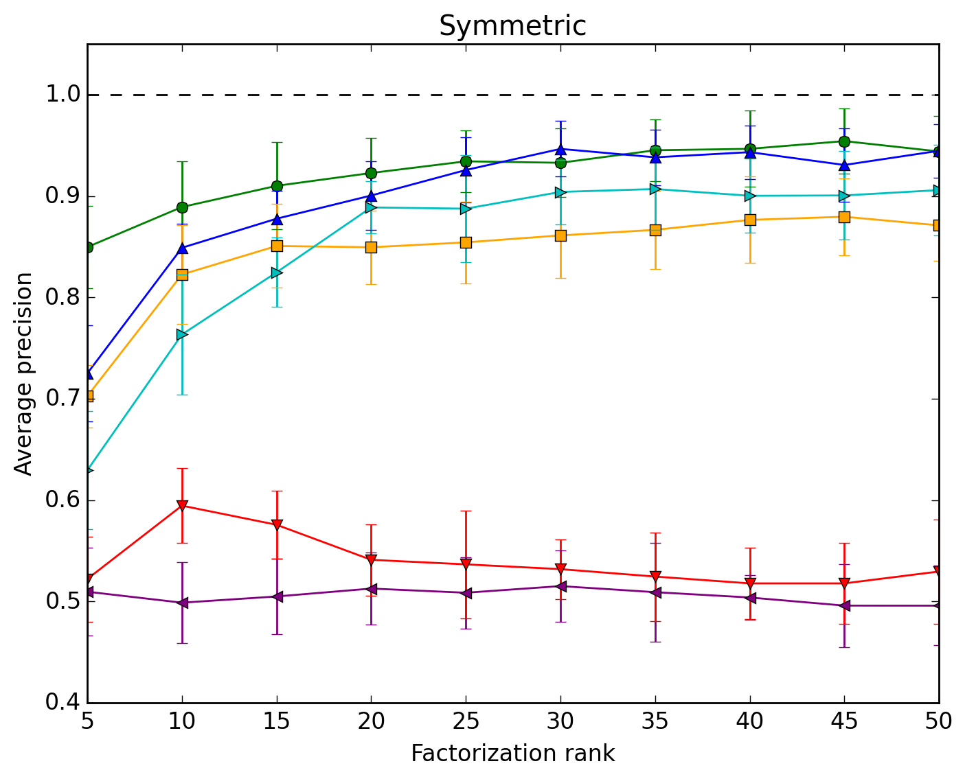
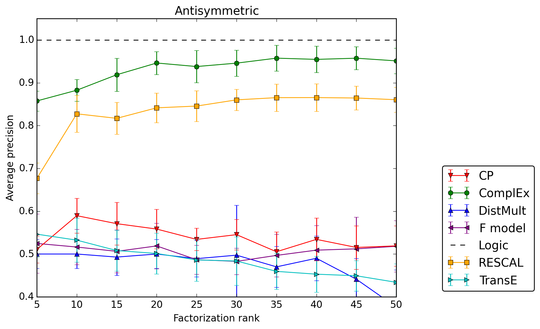
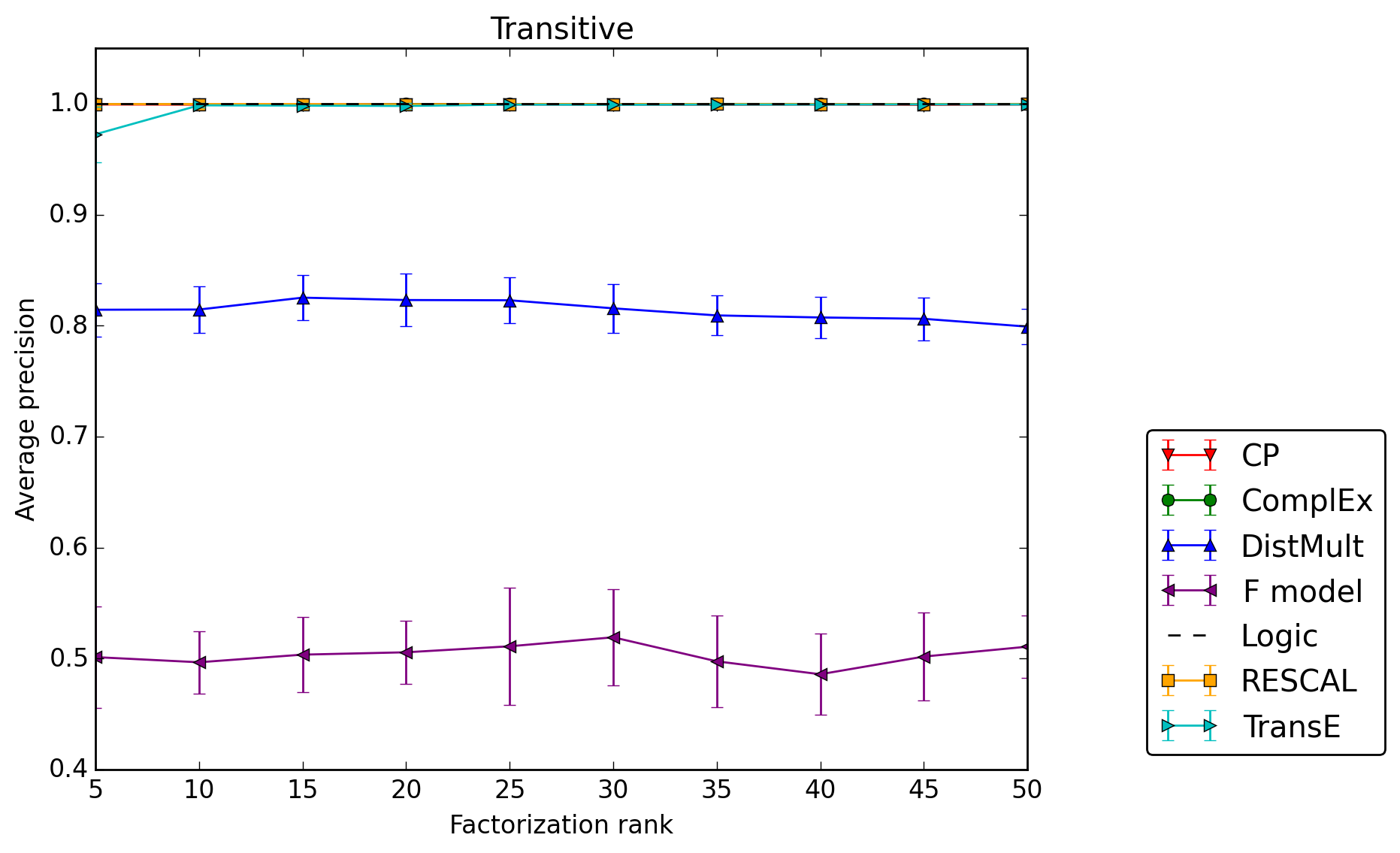
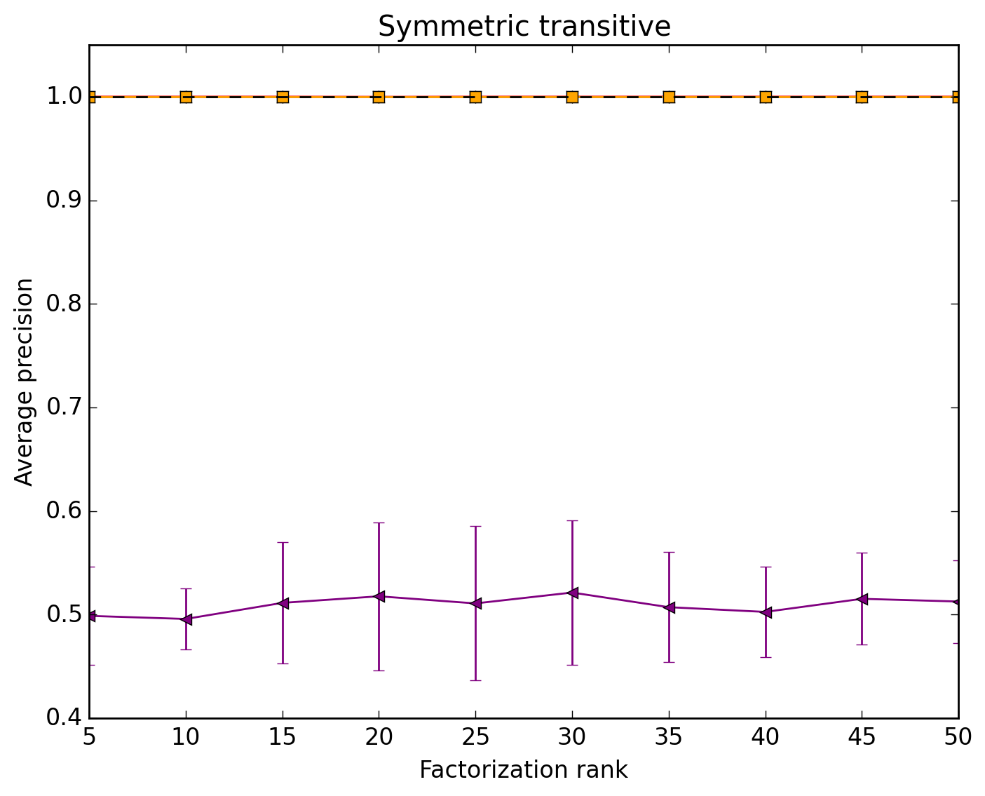
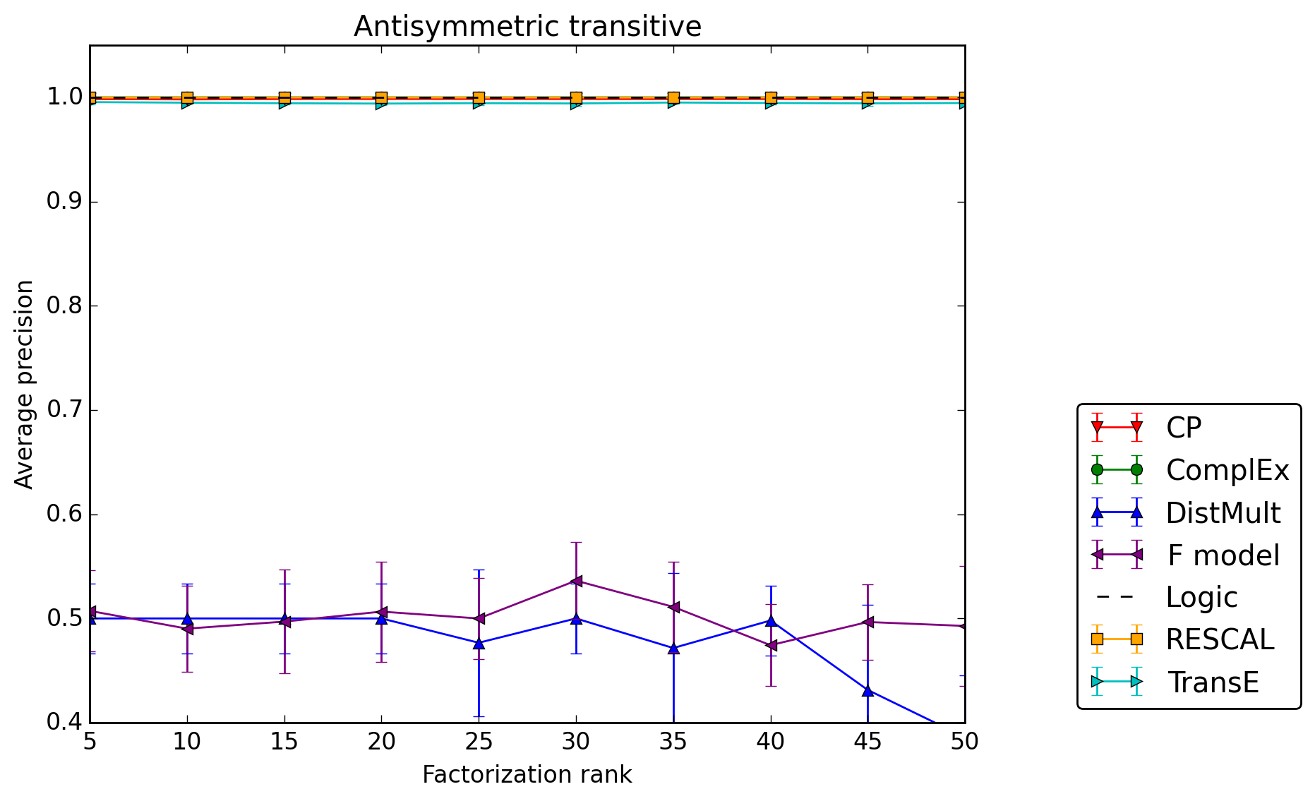
Figure 1 shows the average precision for each model over the generated symmetric and antisymmetric relations. Surprisingly, on such simple relations with 80% of observed data, only ComplEx and RESCAL manage to learn from the symmetric and antisymmetric patterns, with a non-negligible advantage for the ComplEx model. Moreover, we can see that with higher ranks, RESCAL starts overfitting as its average precision decreases presumably due to its quadratic number of parameters with respect to the rank, since each relation $r$ is represented by a matrix $W_{r}\in\mathbb{R}^{K\times K}$, as showed in Equation 4.

The CP model probably fails due to its uncorrelated representations of entities as subject and as objects, which makes it unable to model symmetry and antisymmetry. DistMult unsurprisingly fails in the non-symmetric cases, due to the symmetric nature of its scoring function, and thus succeeds in the symmetric case. More unexpectedly, the TransE model has a hard time on antisymmetry, but performs well on the symmetric relation, by zeroing its relation embedding, as explained in Section 3.2. The F model, cannot actually generalize in a single relation case, as it has one single embedding for each (ordered) entity pair. For any fact $r(s,o)$ in the test set, the entity pair $(s,o)$ has never been seen in the training set, and thus has a random embedding vector.

Figure 3 shows results for the symmetric transitive and antisymmetric transitive relations, and Figure 2 for the transitive only relations. Almost all models, except the F model and DistMult in the non-symmetric cases, perfectly generalize with very low-rank. This tells us that transitivity actually brings so much structure in the data that it makes the problem very easy for latent factor models when most of the data is observed.

Most state-of-the-art latent factor models are surprisingly unable to model all the basic properties of binary relations. Though most of the time those relations are learnt together, but also with much less observed facts. We next assess the models ability to learn these five relations together, and their robustness to sparse observations by gradually decreasing the size of the training set.

4.2.2 Joint Learning

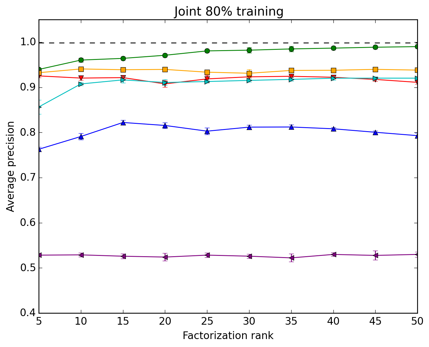
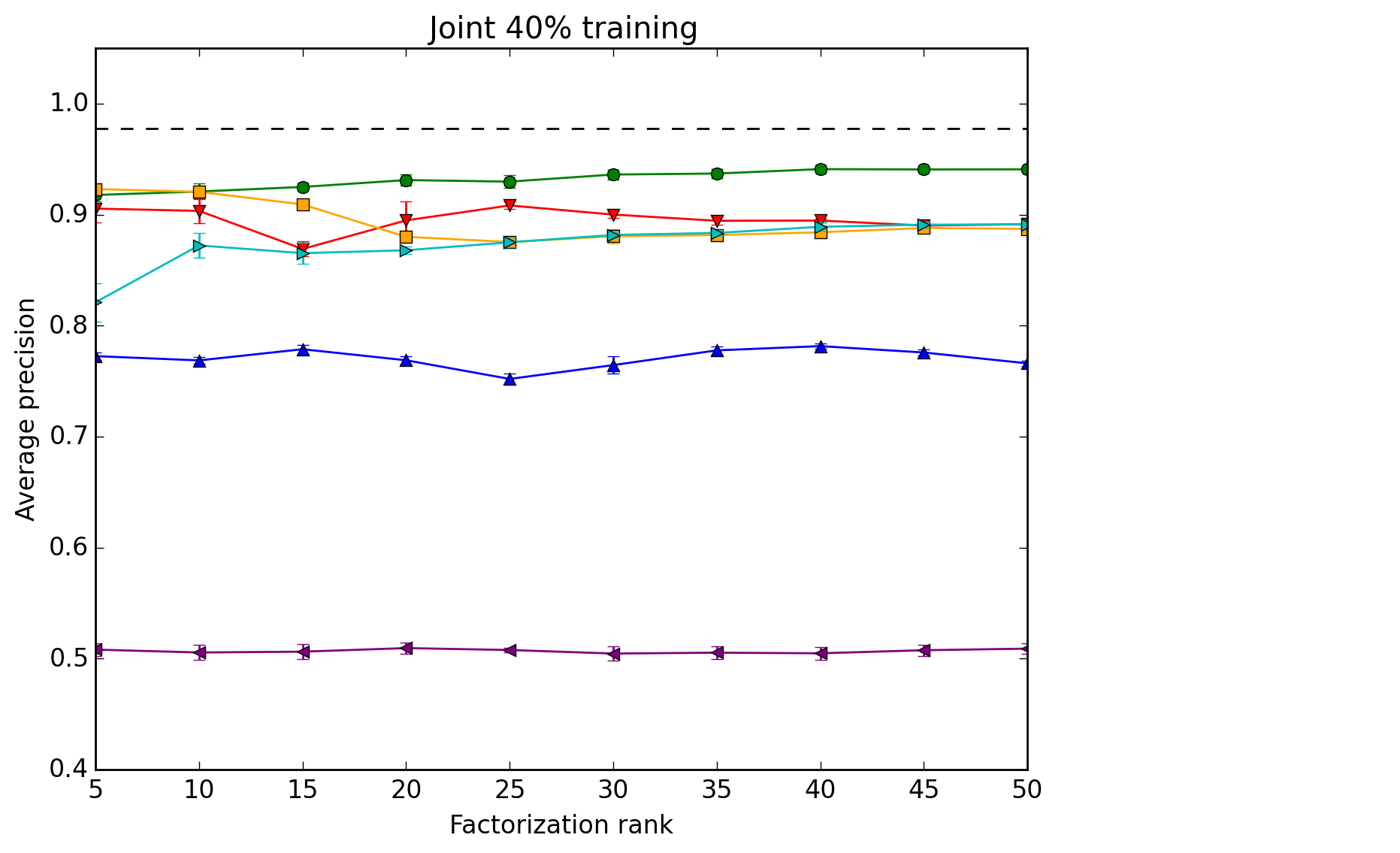
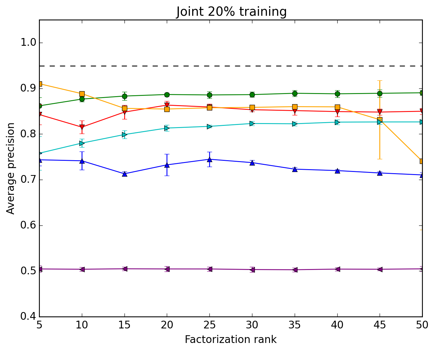
Figure 4 shows the results when all five above relations are jointly learned, for different proportions of the training set: 80%, 40%, 20%, 10%. As expected the scores drop, and the gap between the—deterministic logic—upper-bound and latent factor models widen with the decrease of training data. ComplEx proves to be the most robust to missing data down to 20%, but match logical inference only with 80% of training data.

RESCAL again overfits with the rank increasing, but is the best performing model with 10% of the training set, up to rank $K=30$. This suggests that having richer relation representations than entity representations, that is with more parameters, can be profitable for learning relation properties from little data. However the reason why the variance of RESCAL’s average precision decreases again for $K\geq 40$ remains mysterious.

The CP and TransE models seem to be more sensitive to missing data as their curves progressively get away from RESCAL’s one with the percentage of observed data decreasing. DistMult, being a symmetric model, is below the other models in the four settings as some of the relations are not symmetric.

Since each relation is generated independently, having observed the entity pair $(s,o)$ in the other relations does not help the F model, and it thus fails here too. At 10%, we see that the latent factor models cannot match logical inference, suggesting that the number of examples is not sufficient to learn these properties.

Finally, in the last setting with 10% of the training set, the best models are still 10 points below the best achievable average precision, showing that they need a large amount of training data to correctly learn these basic properties of binary relations.

Figure 4: Joint learning of the 5 relations with 50 entities: one symmetric, one antisymmetric, one transitive, one symmetric and transitive, and one antisymmetric and transitive. Average Precision for each factorization rank ranging from 5 to 50 of each model. Top-Left: 80% train set, Top-Right: 40% train set, Bottom-Left: 20% train set, Bottom-Right: 10% train set.

These results should be taken cautiously as this experiment does not state that in general at least 80% of the facts should be observed in order to learn these properties correctly. Indeed, here the 5 relations are completely uncorrelated, while in real knowledge graphs they generally are correlated and thus share information. Also, as often in machine learning, the ratio between the number of parameters and the number of data points is more informative about generalization than the number of data points alone.

Relation Properties Experiments Summary:

• Only ComplEx manages to learn each combination near perfectly.

• RESCAL is the most robust to missing data with low ranks.

• There is room for improvement on all models when a lot of data is missing.

5 Learning Inter-Relational Patterns: Family Relationships

We generated family trees and their corresponding kinship relations and facts, and designed three different splits of the data. The three splits try to assess different inductive properties of the latent models, by giving more or less supporting facts in the training set.

5.1 Experimental Design

Predicting family relationships is an old task in AI, popularised by Hinton’s kinship data set (cite Hinton, (1986)). Generated synthetic families for testing link-prediction models have also been recently proposed (cite García-Durán et al., (2014)). In this public dataset, generated families are all intertwined with each other in it. We here want each family to be disjoint from the other ones, such that there is no true fact between entities of two different families, and we will see why below.

We propose here to generate family relations from synthetic family trees, namely: mother, father, husband, wife, son, daughter, brother, sister, uncle, aunt, nephew, niece, cousin, grandfather, grandson, grandmother and granddaughter.

Figure 5: Example of a generated family tree.

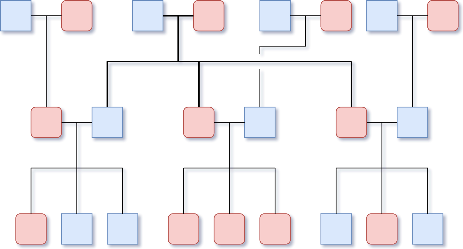
We sample five families independently that span over three generations from a unique couple, with three children per couple of random sex, where husbands, wives and their parents were added to wed the middle generation. Figure 5 shows an example of such a family tree. The whole data set totals 115 entities—23 persons per family—and the 17 relations mentioned above. Each family thus consists in 8993 true and false facts.

$\mathtt{\forall a\forall b\forall c\enspace father(a,c)\wedge mother(b,c)\Rightarrow husband(a,b)}$
$\mathtt{\forall a\forall b\forall c\enspace father(a,c)\wedge mother(b,c)\Rightarrow wife(b,a)}$
$\mathtt{\forall a\forall b\forall c\enspace daughter(a,c)\wedge son(b,c)\Rightarrow sister(a,b)}$
$\mathtt{\forall a\forall b\forall c\enspace daughter(a,c)\wedge son(b,c)\Rightarrow brother(b,a)}$
$\mathtt{\forall a\forall b\forall c\enspace father(a,b)\wedge father(b,c)\Rightarrow grandfather(a,c)}$
$\mathtt{\forall a\forall b\forall c\enspace son(a,b)\wedge son(b,c)\Rightarrow grandson(a,c)}$
$\mathtt{\forall a\forall b\forall c\enspace mother(a,b)\wedge mother(b,c)\Rightarrow grandmother(a,c)}$
$\mathtt{\forall a\forall b\forall c\enspace daughter(a,b)\wedge daughter(b,c)\Rightarrow granddaughter(a,c)}$
$\mathtt{\forall a\forall b\forall c\forall d\enspace son(a,b)\wedge daughter(b,c)\wedge son(d,c)\Rightarrow uncle(d,a)}$
$\mathtt{\forall a\forall b\forall c\forall d\enspace daughter(a,b)\wedge son(b,c)\wedge daughter(d,c)\Rightarrow aunt(d,a)}$
$\mathtt{\forall a\forall b\forall c\forall d\enspace son(a,b)\wedge daughter(b,c)\wedge son(d,c)\Rightarrow nephew(a,d)}$
$\mathtt{\forall a\forall b\forall c\forall d\enspace daughter(a,b)\wedge son(b,c)\wedge daughter(d,c)\Rightarrow niece(a,d)}$
$\mathtt{\forall a\forall b\forall c\forall d\forall e\enspace son(a,b)\wedge daughter(b,c)\wedge son(d,c)\wedge daughter(e,d)\Rightarrow cousin(a,e)}$

Table 4: Examples of rules to deduce all relations from the four relations: mother, father, son and daughter.

Within these traditional families that feature only married heterosexual couples that do not divorce and have children, one can figure out that the relations mother, father, son and daughter are sufficient to deduce the 13 remaining ones. Examples of rules that allow deducing these 13 relations from the 4 main ones are shown in Table 4. From this fact, we devise three different splits of the data.

Let us first introduce notations for each subset of the observed facts set $\Omega$. As each family is independent from the four others, we will denote each entity set of each family from 1 to 5: $\mathcal{E}^{1},\ldots,\mathcal{E}^{5}$, where $\mathcal{E}^{i}\cap\mathcal{E}^{j}=\emptyset$ with $i\neq j$. Accordingly, we will write the observed facts of each family $\Omega^{1},\ldots,\Omega^{5}$, where for all $((r,s,o),y_{rso})\in\Omega^{i}$ we have $s,o\in\mathcal{E}^{i}$. Observed fact sets that contain only the 4 main relations mother, father, son and daughter are denoted by $\Omega_{\mathrm{4main}}$, and the facts involving the 13 other relations by $\Omega_{\mathrm{13other}}$. We thus have for each family $i$: $\Omega^{i}=\Omega^{i}_{\mathrm{4main}}\cup\Omega^{i}_{\mathrm{13other}}$. Figure 6 draws the corresponding tensor with each subset of the observed facts. Finally, let the sampling function $\mathcal{S}_{p}(\Omega)$ be a uniformly random subset of $\Omega$ of size $|\mathcal{S}_{p}(\Omega)|=\lceil p|\Omega|\rceil$, with $0\leq p\leq 1$, $p$ being the proportion of the set that is randomly sampled.

Figure 6: Tensor representation of the observed subsets for the family experiments. The part in dark orange represents the sets containing the four relations mother, father, son and daughter, while the part in light orange represents the 13 other relations.

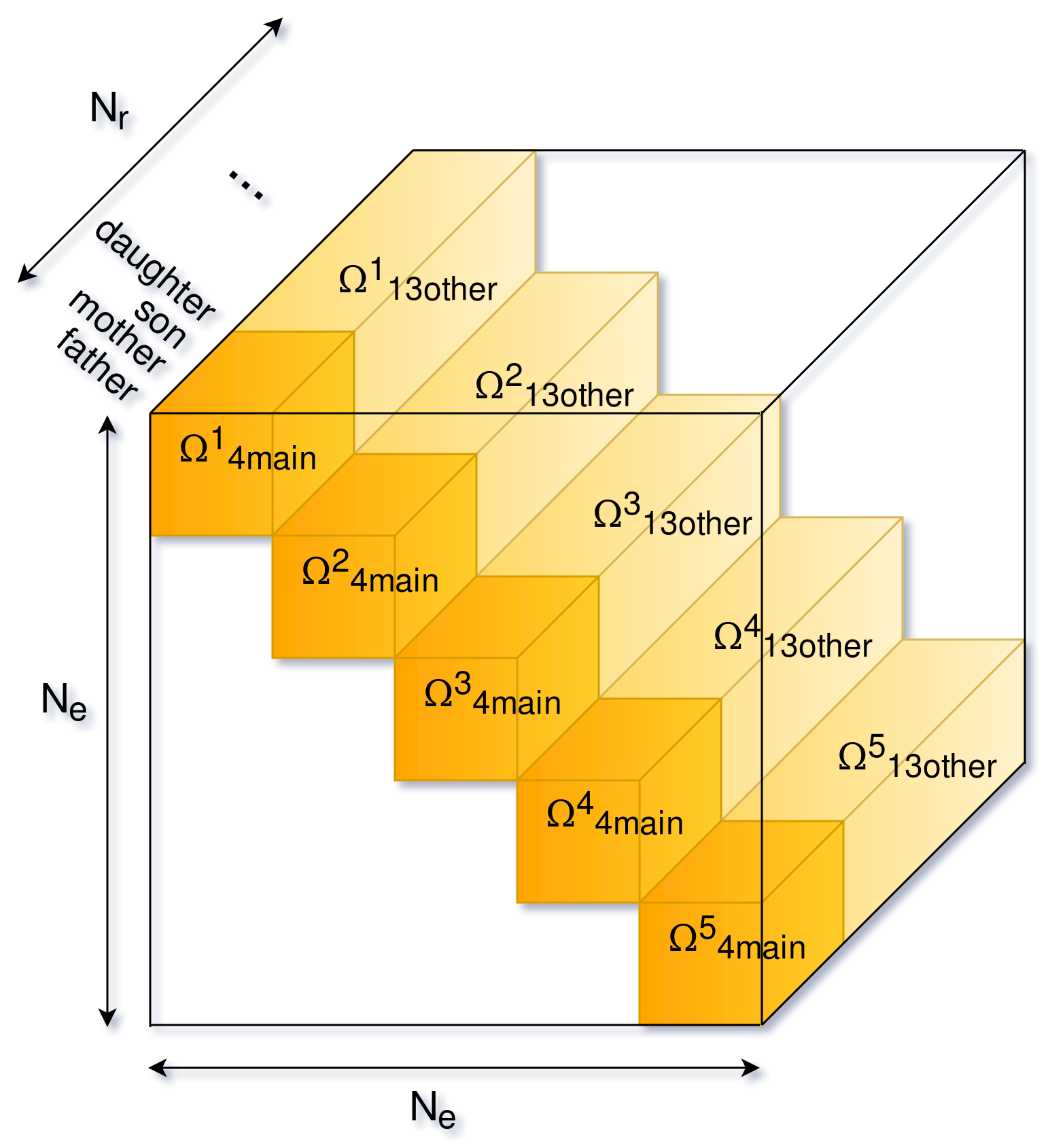
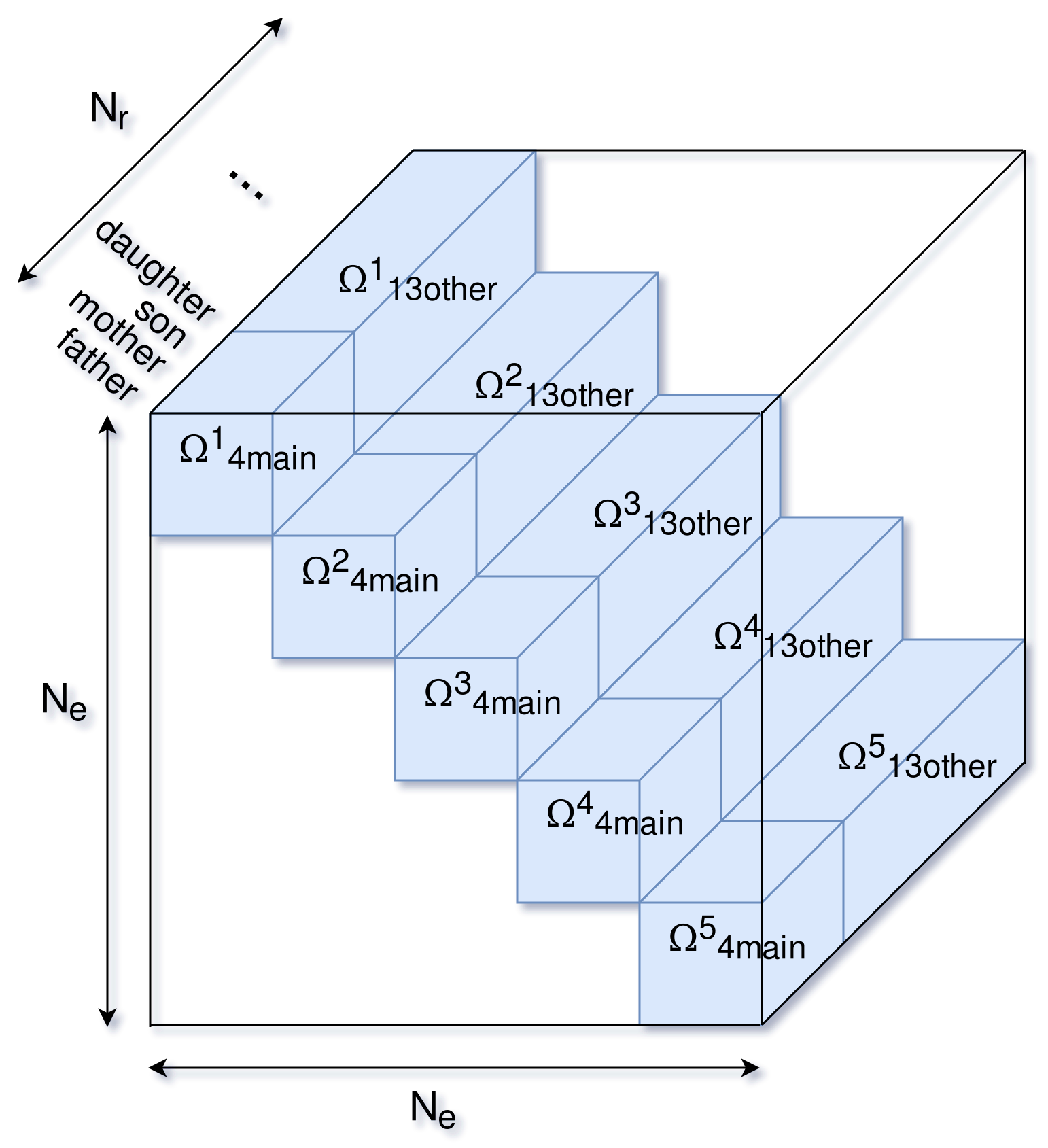
We propose to split the data in three different ways to explore inductive abilities of the models. The first split is the classical random split between training, validation and test sets, it will mainly serve as a control experiment for the other splits. In the second split, we aim at evaluating whether latent factor models are able to leverage this information. To do so, we ensure that all the relations mother, father, son and daughter of the five families are in the training set, and we split the 13 remaining ones between training, validation and test set. Formally: $\Omega_{\mathrm{train}}=\Omega_{\mathrm{4main}}\cup\mathcal{S}_{p}(\Omega_{\mathrm{13other}})$. We will call this splitting scheme the evidence split, as the training set always contains the sufficient evidence to deduce the 13 other relations—that is the four main ones.

Thirdly, we assess the ability of latent factor models to transfer knowledge learnt from a family to another, that is between disjoint set of entities. In this split, the training set always contains all the relations for four out of the five families plus all the mother, father, son and daughter of the fifth family, while the 13 other relations of this fifth family are split between training, validation and test set. Formally: $\Omega_{\mathrm{train}}=\Omega^{1-4}\cup\Omega^{5}_{\mathrm{4main}}\cup\mathcal{S}_{p}(\Omega^{5}_{\mathrm{13other}})$. We will call it the family split. Figure 7 shows tensor drawings of the three splits.

(a) Random split

(b) Evidence split

(c) Family split

Figure 7: Tensor representation of the three different splits. Green sets are always contained in the training set $\Omega_{\mathrm{train}}$, whereas blue sets are split among training, validation and test sets.

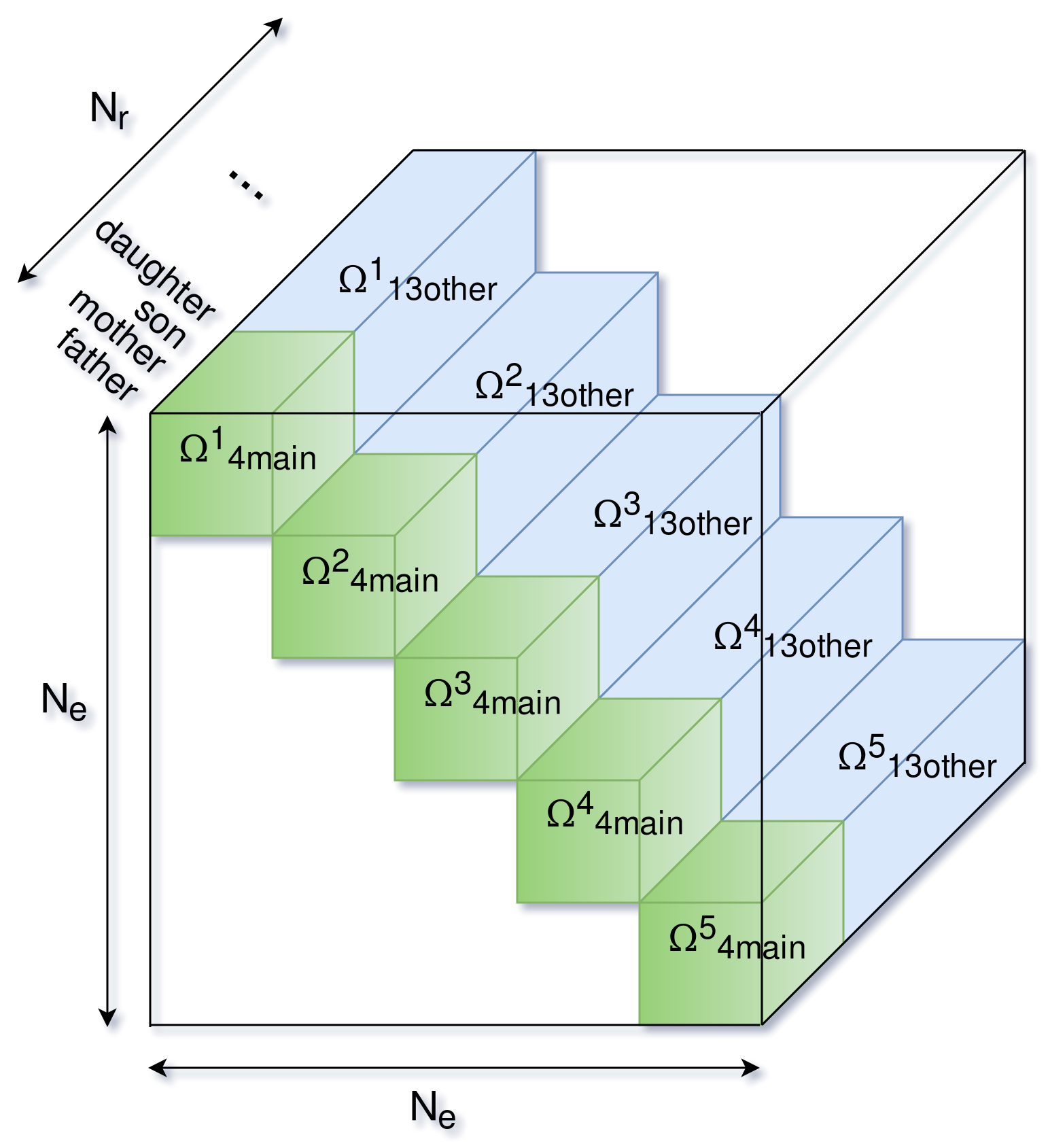
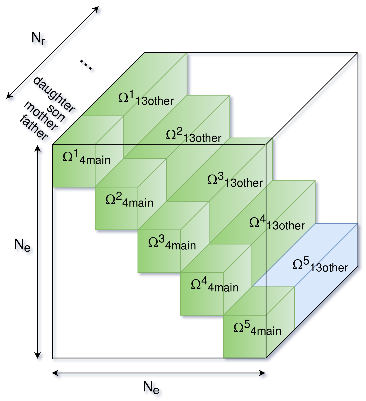
For each split we explore different values of $p\in\{0.8,0.4,0.2,0.1\}$. We also run with $p=0$ in the last (family) split, which corresponds to $\Omega_{\mathrm{train}}=\Omega^{1-4}\cup\Omega^{5}_{\mathrm{4main}}$, that is 4 entirely observed family, plus the 4 main relations of the fifth one. Observe that it only makes sense to have $p=0$ in this last split. If latent factor models have expected inductive abilities, they would be able to understand genealogical reasoning from the four first families, and use this learned information to correctly predict the 13 other relations of the fifth family from its four main ones. Note that in the last two splits, a deterministic logic inference system makes perfect predictions—given rules such as the ones shown in Table 4—for any value of $p$. The number of facts in the training, validation and test sets of each split are summarized in Table 5.

		Size with $p=$
Split	Set	0.8	0.4	0.2	0.1	0
Random	$\Omega_{\mathrm{train}}=\mathcal{S}_{p}(\Omega)$	35973	17987	8994	4496	-
	$\Omega_{\mathrm{valid}}=\mathcal{S}_{0.1}(\Omega)$	4496	4496	4496	4496	-
	$\Omega_{\mathrm{test}}=\mathcal{S}_{(0.9-p)}(\Omega)$	4496	22482	31475	35973	-
Evidence	$\Omega_{\mathrm{train}}=\Omega_{\mathrm{4main}}\cup\mathcal{S}_{p}(\Omega_{\mathrm{13other}})$	38089	24334	17457	14019	-
	$\Omega_{\mathrm{valid}}=\mathcal{S}_{0.1}(\Omega_{\mathrm{13other}})$	3438	3438	3438	3438	-
	$\Omega_{\mathrm{test}}=\mathcal{S}_{(0.9-p)}(\Omega_{\mathrm{13other}})$	3438	17193	24070	27508	-
Family	$\Omega_{\mathrm{train}}=\Omega^{1-4}\cup\Omega^{5}_{\mathrm{4main}}\cup\mathcal{S}_{p}(\Omega^{5}_{\mathrm{13other}})$	43589	40839	39463	38776	38088
	$\Omega_{\mathrm{valid}}=\mathcal{S}_{0.1}(\Omega^{5}_{\mathrm{13other}})$	688	688	688	688	688
	$\Omega_{\mathrm{test}}=\mathcal{S}_{(0.9-p)}(\Omega^{5}_{\mathrm{13other}})$	688	3438	4814	5501	6189

Table 5: Training, validation and test set numbers for each split for each value of $p$.

Similar splits of data have already been proposed to evaluate rule-based inference models (for example the UW-CSE dataset (cite Richardson and Domingos, (2006))), which are able of such transfer of reasoning between disjoint sets of entities. Interestingly, such data sets have rarely been reused in the subsequent latent factor model literature. Results reported next might give us a hint why this is the case.

5.2 Results

Results are reported for each split separately. In each of them we again decrease progressively the amount of training data.

5.2.1 Random Split

Figure 8: Average Precision for each factorization rank ranging from 5 to 50 of each model on the families experiment with the random split. Top-left: $p=0.8$, top-right: $p=0.4$, bottom-left: $p=0.2$, bottom-right: $p=0.1$.

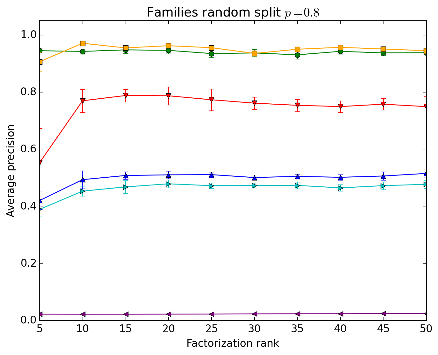
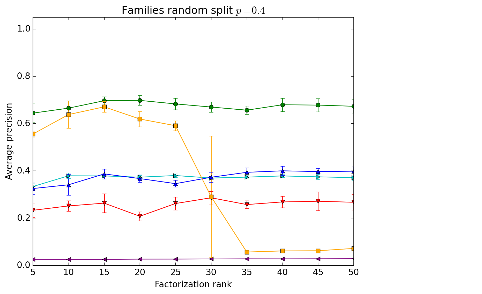
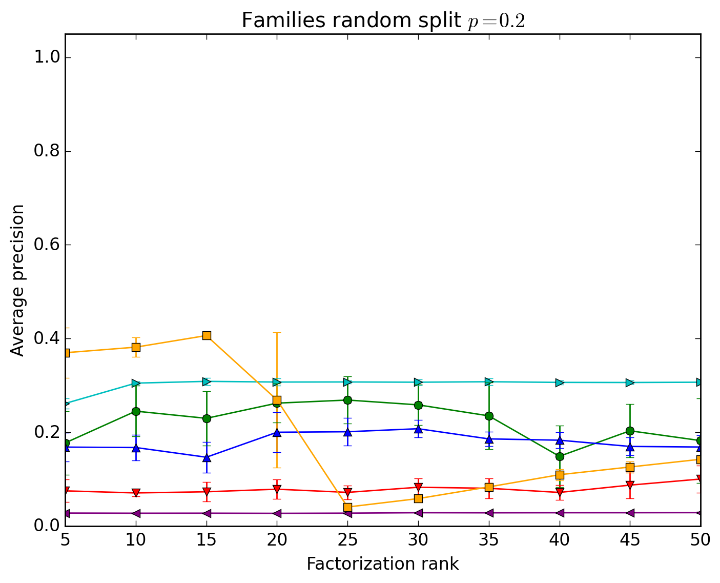
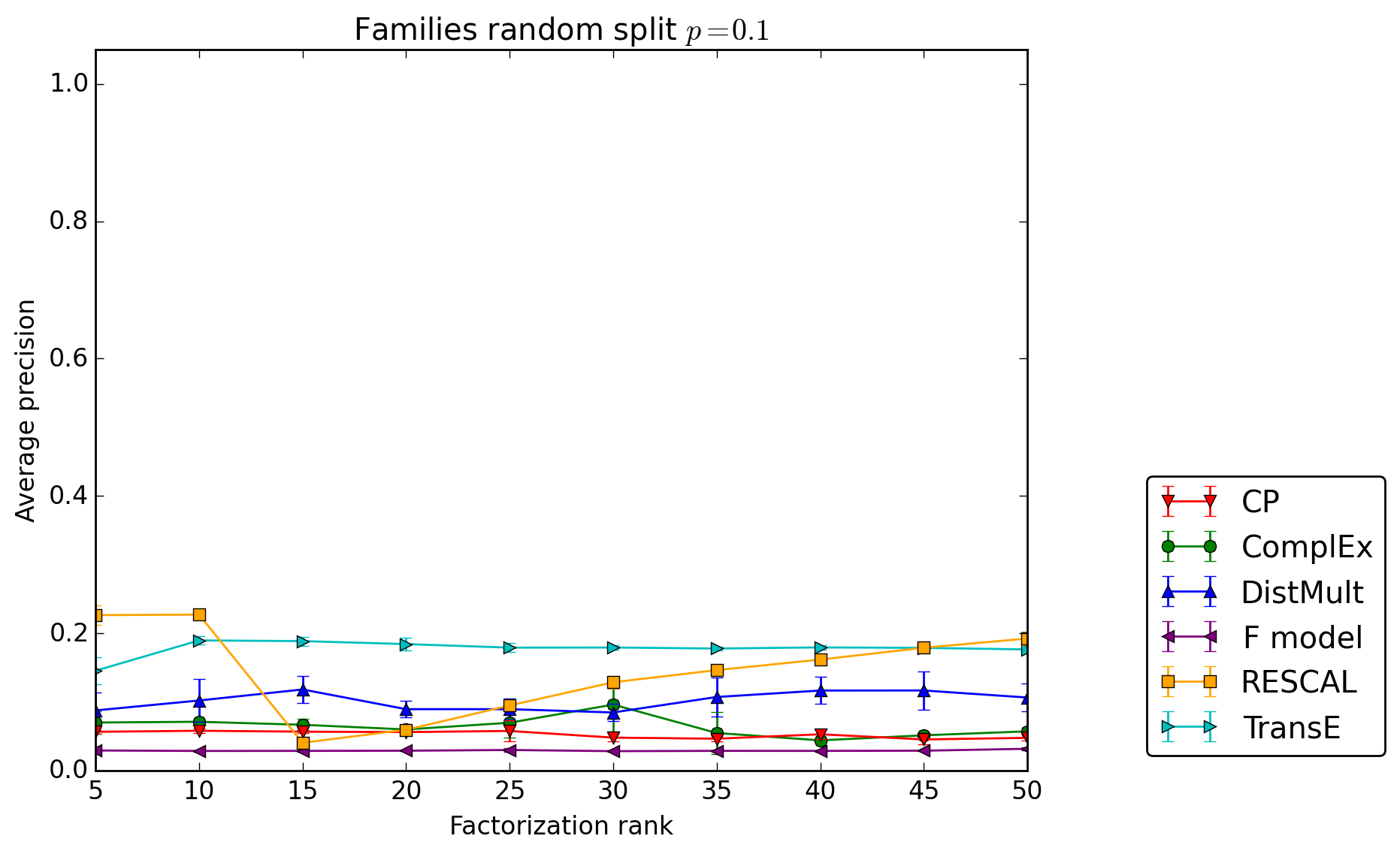
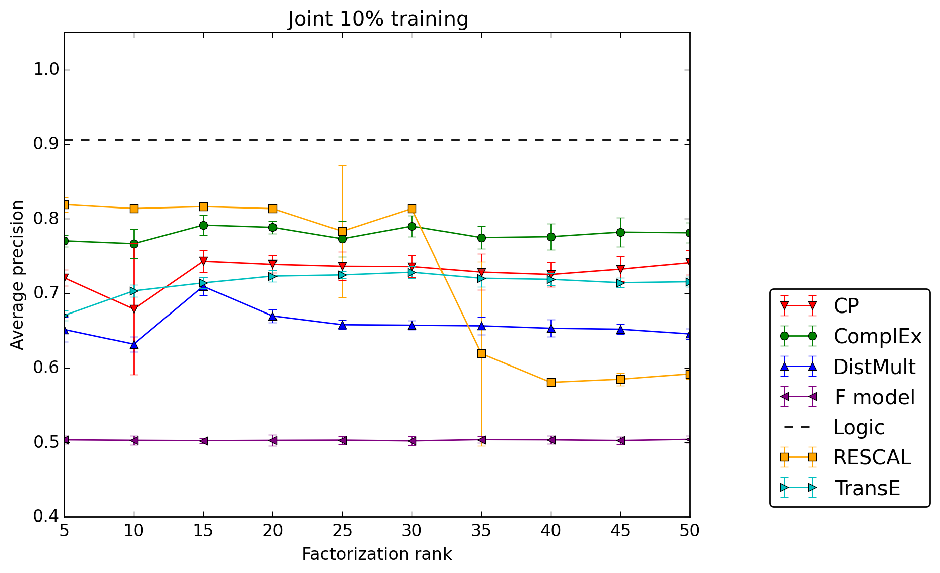
In the first random split, we try to evaluate the quantity of training data needed to learn to reason in genealogies. Figure 8 shows the average precision of each model for ranks ranging from 5 to 50, for each value of $p$. Only ComplEx and RESCAL are able to generalize almost perfectly with 80% of observed data, which first tells us that these models are indeed capable to learn such genealogical reasonings. As many relations are antisymmetric, it is no surprise that DistMult and TransE cannot reach perfect predictions, as they already failed in the antisymmetric synthetic relation.

The ComplEx model generalizes quickly with small ranks, but is outrun by RESCAL—with small ranks—and TransE when the percentage of observed data decreases below $p=0.2$. We conjecture that TransE’s robustness is due to its bilinear terms, and especially the one that involves the subject and the object embeddings—$e_{s}^{\top}e_{o}$—as shown in Equation 7, that can give high scores to pairs of entities belonging to the same family. For RESCAL, its richer representations of relations by matrices probably help here, as long as the rank is not too big which clearly causes overfitting.

The CP decomposition scores drop quickly with the proportion of observed data, because of its unrelated subject and object representations. The F model here fails again, for a simple reason: these relations are exclusive between themselves for a given pair of entities $(s,o)$. Indeed, if father($s,o$) is true for example, then none of the other relations between $s$ and $o$ will be true—at least not in these families. Hence if the F model has to predict the score of the fact $r(s,o)$, it has no other true triple involving $(s,o)$ to support its decision. It will also have troubles on the two next splits for the same reason. Note that in this split, the logic upper-bound is not given as one would need to know all possible rules to deduce the 17 relations from each of them—and not only from the four main ones—to compute this upper-bound.

5.2.2 Evidence Split

In this split, we recall that all the mother, father, son and daughter relations are always in the train set for the 5 families. The value of $p$ ranging from 0.8 to 0.1 corresponds here to the proportion of the 13 other relations that are also put into the training set. The test and validation sets are only composed of these 13 relations.

Figure 9: Average Precision for each factorization rank ranging from 5 to 50 of each model on the families experiment with the evidence split. Top-left: $p=0.8$, top-right: $p=0.4$, bottom-left: $p=0.2$, bottom-right: $p=0.1$.

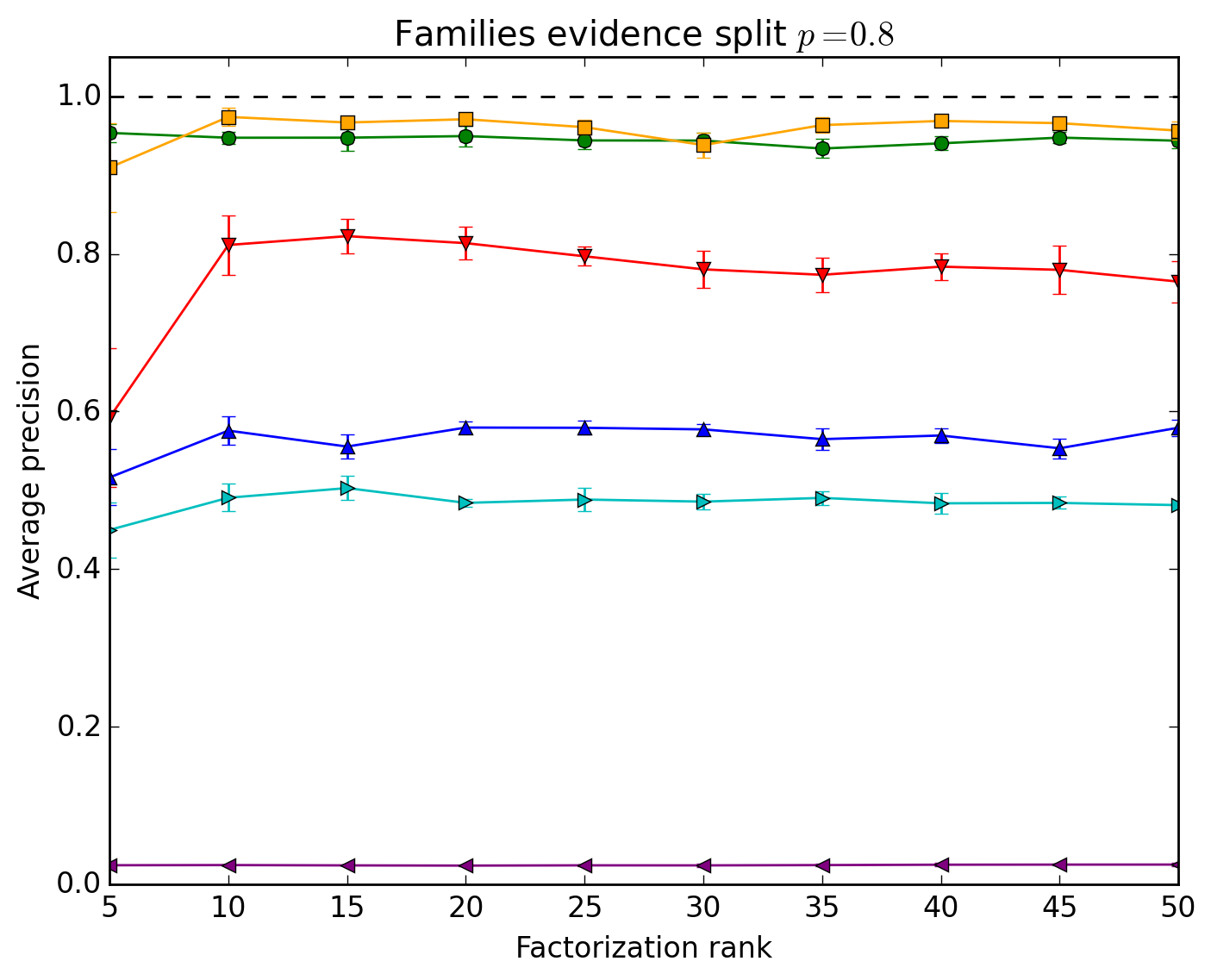
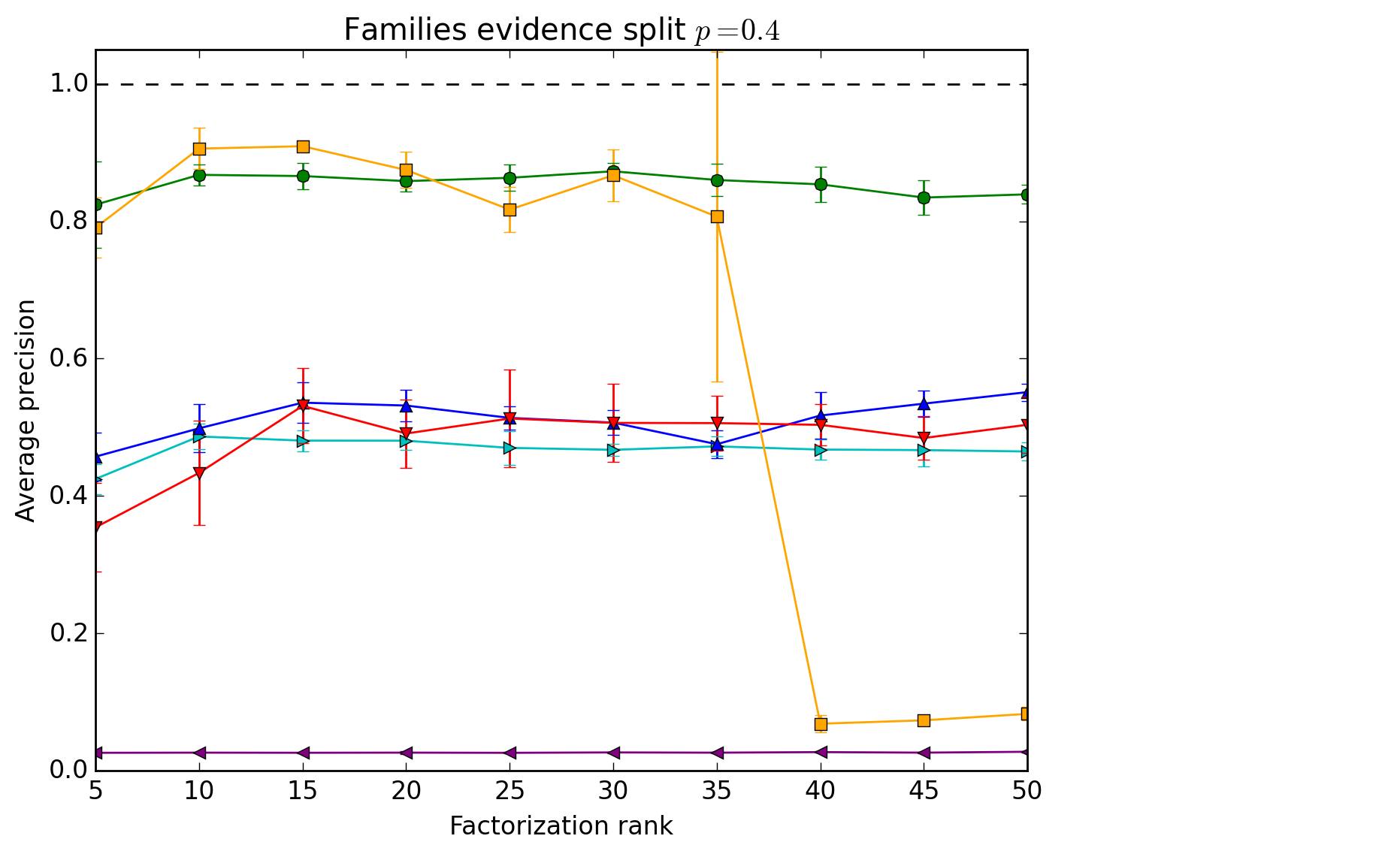
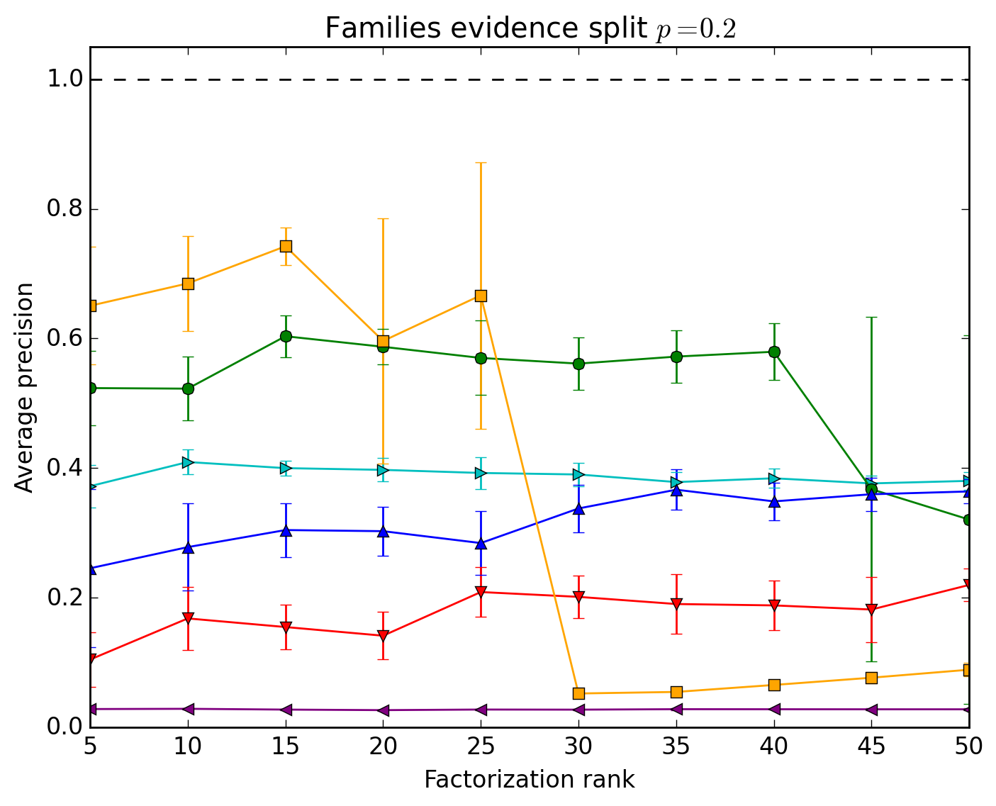
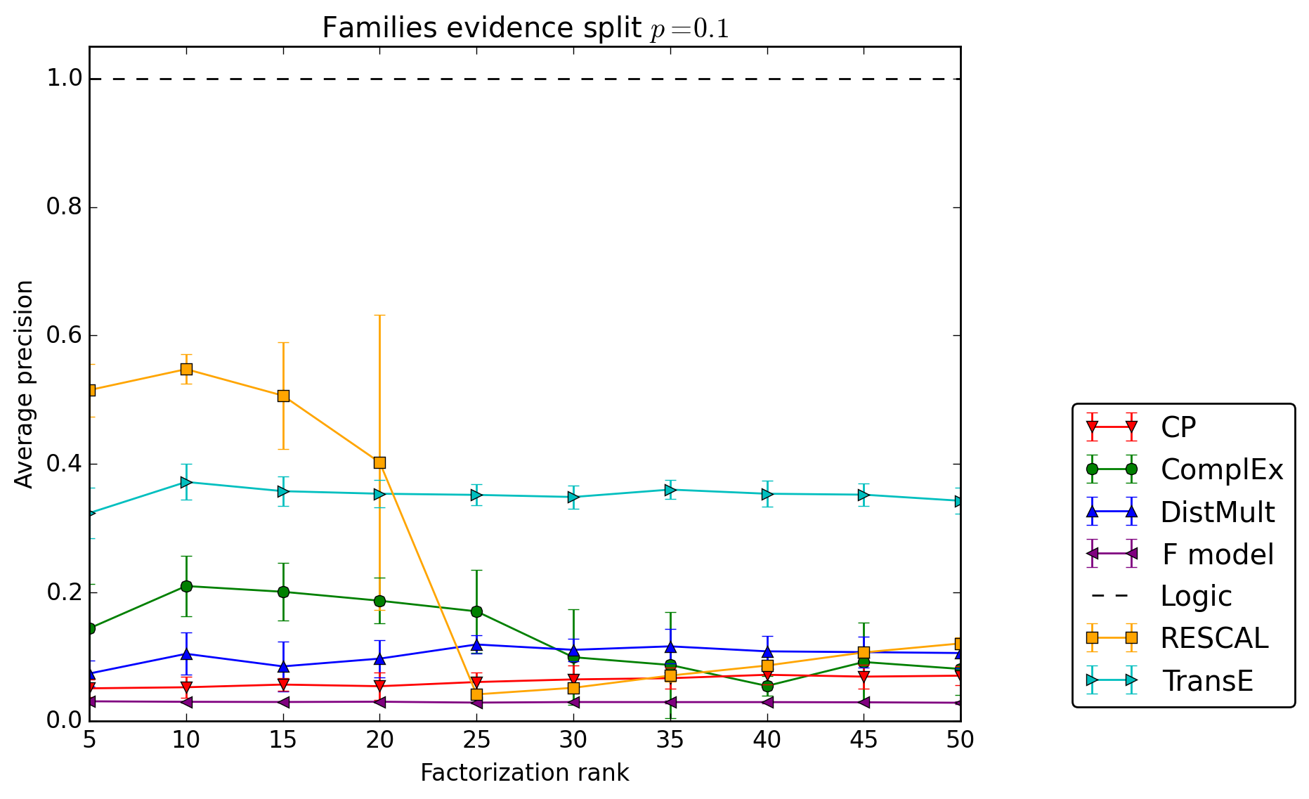
Compared to the random split setting, we can see in Figure 9 that the performances of the models decrease more slowly with the percentage of observed data. This shows that latent factor models are able to use the information provided by these four relations from which all of the others can be deduced.

RESCAL is here clearly the best model for all values of $p$, as long as $K$ is not too big. It exhibits again a behavior that seems to have two equilibria distributed around a pivotal $K$ at which average precision suddenly drops, with high variance of the predictions around that $K$. ComplEx also seems to show a lighter overfitting with high values of $K$ when $p\leq 0.2$. TransE confirms an advantage with $p=0.1$ with a notable rise of average precision compared to the random split. CP, DistMult and the F model fail again for the same reasons as in the random split.

However, given the rules to deduce the 13 other relations from the four main ones, recall that a logical inference engine is able to reach an average precision of one. Though improvement compared to the random split setup is large, the gap with logical inference is still wide with $p=0.1$ and $p=0.2$, showing that latent factor models have troubles making the link between the four main relations and the 13 other ones when limited training data is available. This could be due to the imbalance in the number of each relation in the training set that this split introduces, biasing the entity embeddings towards a better reconstruction of the 4 main relations, to the detriment of the generalization over the 13 remaining ones. Weighting the facts in accordance with the preponderance of each relation in the dataset could improve performances here.

5.2.3 Family Split

In this last split, all the mother, father, son and daughter are in the train set for all families, but also all the 13 other relations of four out of the five families. The value of $p$ corresponds here to the amount of the 13 other relations of the fifth family only that are in the training set too.

Figure 10: Average Precision for each factorization rank ranging from 5 to 50 of each model on the families experiment with the family split. Top-left: $p=0.8$, top-right: $p=0.4$, middle-left: $p=0.2$, middle-right: $p=0.1$, bottom: $p=0.0$.

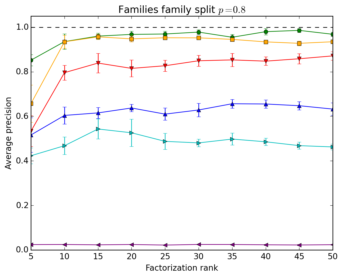
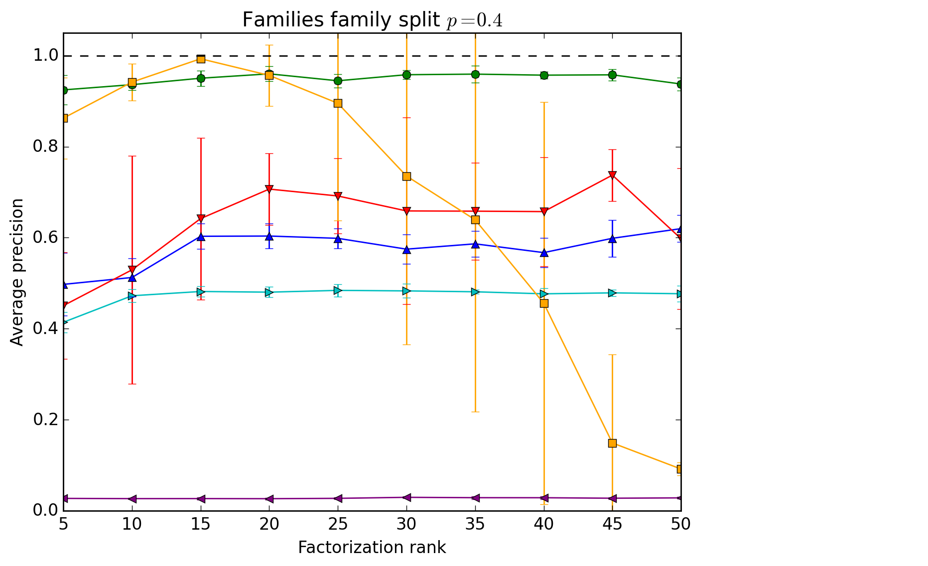
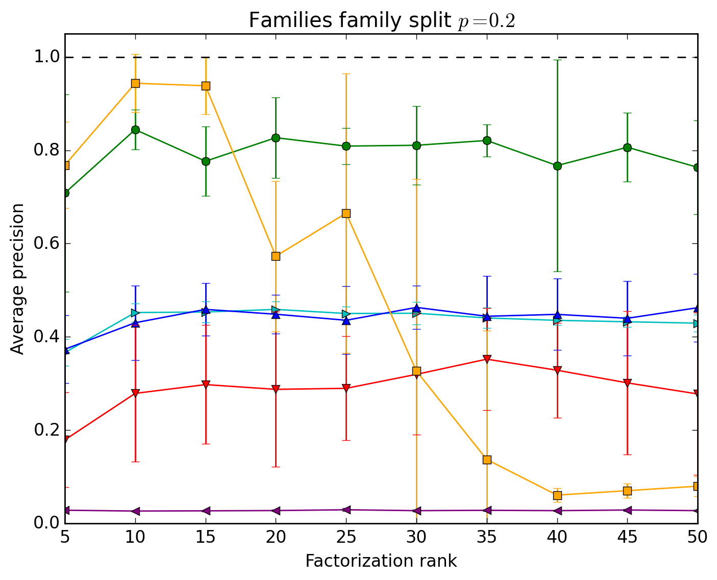
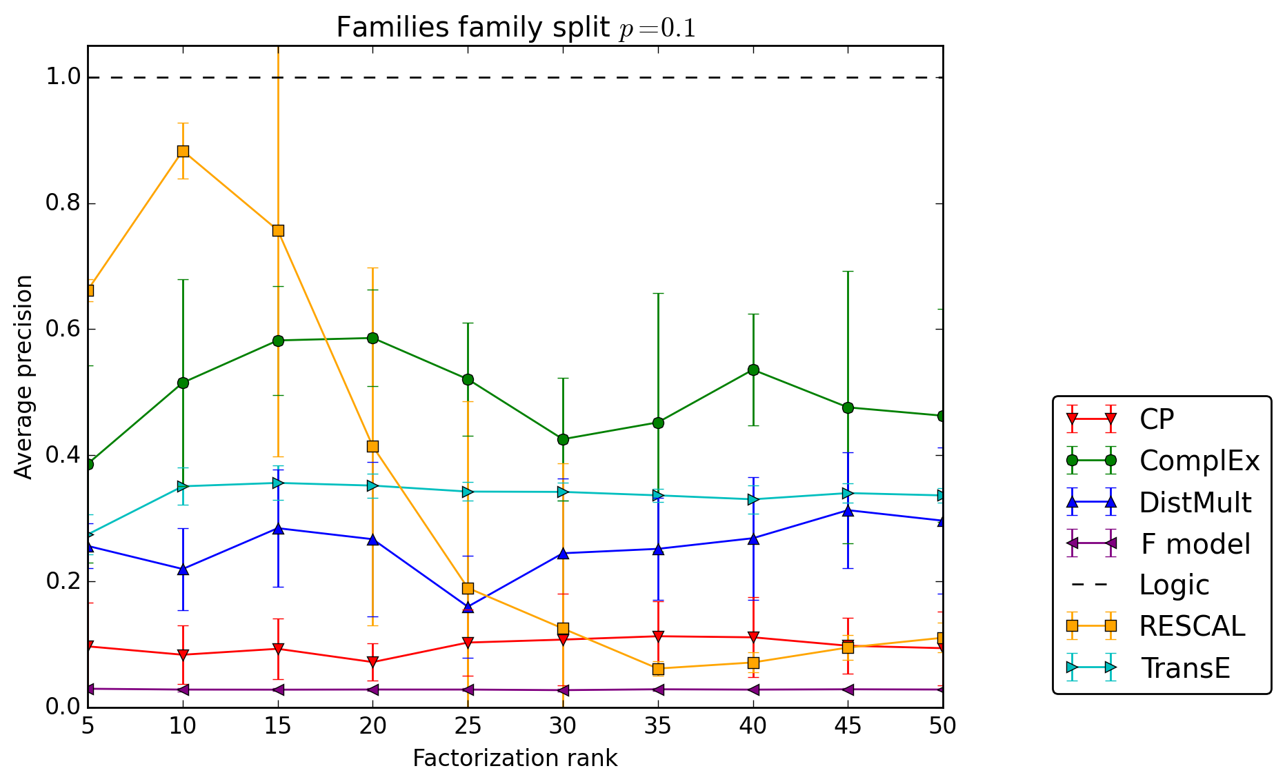
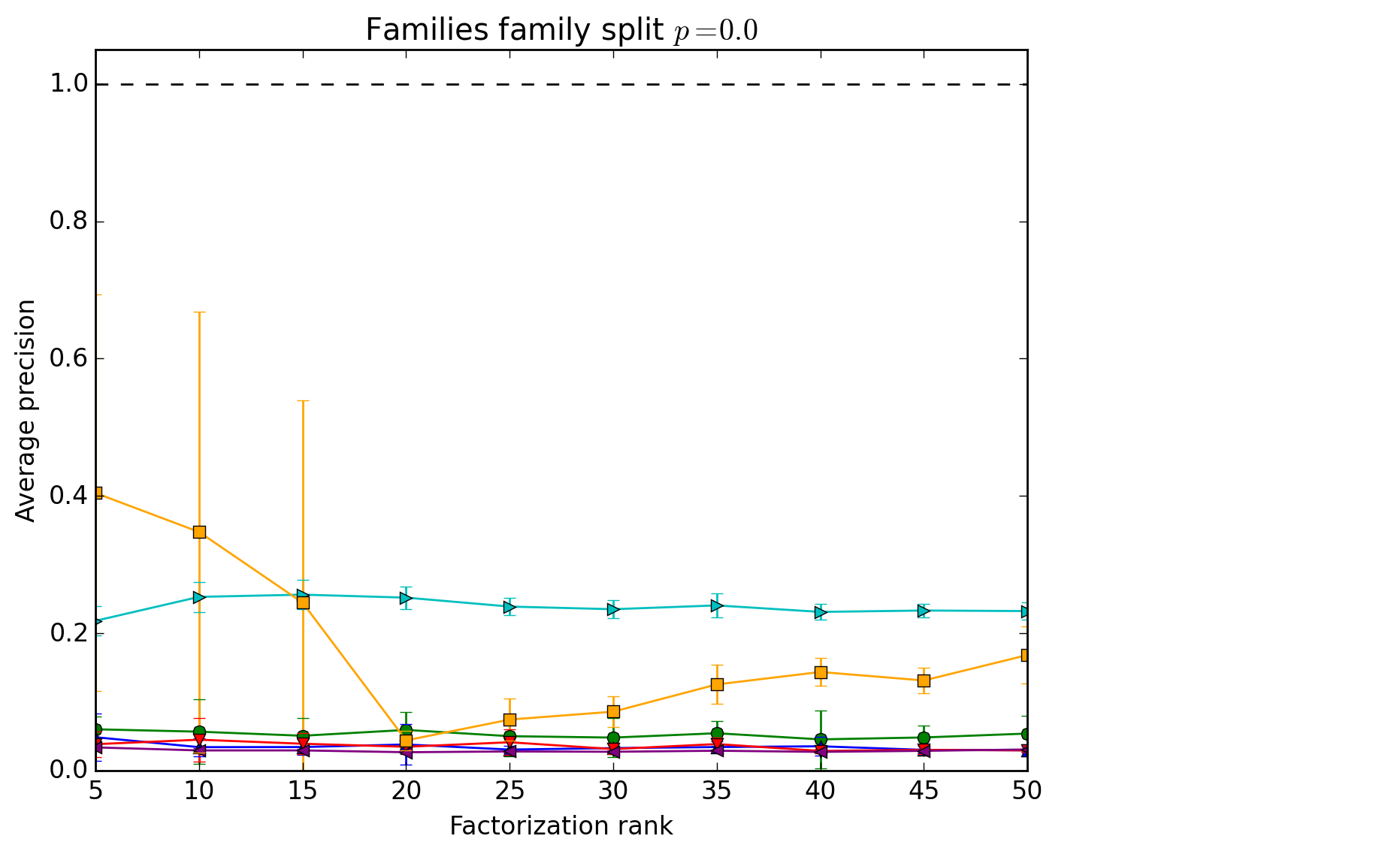
The curves in Figure 10 show a clear improvement over the previous ones in Figure 9. RESCAL is again the best model as it reaches average precisions $\geq 0.9$ even down to $p=0.1$—with small ranks again. ComplEx is in these cases the best with high ranks, though much below RESCAL’s best scores when $p=0.1$.

Does that mean these models were able to exploit the additional information? Yes and no. We conjecture that the better results for $p$ ranging from 0.8 to 0.1 are partly due to the relation imbalance problem—explained in the previous split—being much smaller here, as all the relations of four families are given in in the training set.

To ensure that models indeed did not generalized from the four perfectly informed families, we reduced the proportion $p$ of the 13 other relations of the fifth family that are in the training set to zero—which thus constitute the whole validation and test sets. And though the models are provided with four perfectly informed families, and all the needed facts to predict the missing ones in the fifth family, they fail in this last setting as shown in the bottom plot of Figure 9. RESCAL and TransE resist better than the other models again in this last setting with $p=0$.

This is easily explained, as disconnected sets of entities, here families, correspond to different blocks in the tensor $\mathbf{Y}$, as shown in Figure 6. Entities that are in different families $s,o\in\Omega^{i}$, $s^{\prime},o^{\prime}\in\Omega^{j}$, $i\neq j$, are never involved together in an observed fact: $((s,r,o^{\prime}),y_{sro^{\prime}}),((s^{\prime},r,o),y_{s^{\prime}ro})\notin\Omega$, for any relation $r\in\mathcal{R}$. Thus when learning their embeddings $e_{s},e_{o}$ and $e_{s^{\prime}},e_{o^{\prime}}$, the only link they share is the embedding of the relation $r$ that is involved in the scoring functions $\phi(r,s,o)$ and $\phi(r,s^{\prime},o^{\prime})$. This interpretation is also supported by RESCAL scores, which benefits from its higher number of parameters of its relation representations $W_{r}\in\mathbb{R}^{K\times K}$, which increases the amount of information shared across the families.

To formally bring this problem to light, let us re-frame the tensor approximation problem as a system of inequalities. As $P(y_{rso}=1)=\sigma(\phi(r,s,o;\Theta))$, true triples should have a score $\phi(r,s,o;\Theta)>0$, and false triples $\phi(r,s,o;\Theta)<0$. For the sake of the example, we will consider factorizing the two relations sister and grandfather, with two families of 2 persons each, using the DistMult model. Observing the true fact sister(a,b) or the true fact sister(b,a) where $a,b\in\mathcal{E}$, allows us to deduce that $a$ and $b$ are not the grandfather of each other:

• $\mathtt{sister(a,b)\Rightarrow\neg grandfather(a,b)}$

• $\mathtt{sister(a,b)\Rightarrow\neg grandfather(b,a)}$

• $\mathtt{sister(b,a)\Rightarrow\neg grandfather(a,b)}$

• $\mathtt{sister(b,a)\Rightarrow\neg grandfather(b,a)}$

Similarly to the family split with $p=0$, let us have both relations fully observed for a first family that contains entities $a,b\in\mathcal{E}^{1}$, and only the facts of the relation $\mathtt{sister}$ observed for entities of a second family $c,d\in\mathcal{E}^{2}$. The resulting $2\times 4\times 4$ partially observed binary tensor is:

$$\mathtt{sister}:\blockarray{ccccc}&abcd\\ \block{c(cccc)}a-1\phantom{-}1\\ b\phantom{-}1-1\\ c-1\phantom{-}1\\ d\phantom{-}1-1\\ \,,\qquad\mathtt{grandfather}:\blockarray{ccccc}&abcd\\ \block{c(cccc)}a-1-1\\ b-1-1\\ c\cdot\cdot\\ d\cdot\cdot\\$$ (11)

where $\cdot$ and empty spaces are unobserved facts. From the first, fully observed family we wish to learn the above rules and the irreflexivity of the grandfather relation, to correctly complete the grandfather facts between entities $c$ and $d$.

As the observed blocks—and the block we wish to recover—are symmetric here, there is no expressiveness issue with using DistMult. Decomposing this tensor with the DistMult model with $K=2$ such that true facts have probability $P(y_{rso}=1)>0.5$ and false facts have probability $P(y_{rso}=1)<0.5$, amounts to solving the following system of inequalities:

$$\begin{cases}w_{s1}^{\phantom{2}}e_{a1}^{2}+w_{s2}^{\phantom{2}}e_{a2}^{2}<0\\ w_{s1}^{\phantom{2}}e_{b1}^{2}+w_{s2}^{\phantom{2}}e_{b2}^{2}<0\\ w_{s1}e_{a1}e_{b1}+w_{s2}e_{a2}e_{b2}>0\\ w_{g1}^{\phantom{2}}e_{a1}^{2}+w_{g2}^{\phantom{2}}e_{a2}^{2}<0\\ w_{g1}^{\phantom{2}}e_{b1}^{2}+w_{g2}^{\phantom{2}}e_{b2}^{2}<0\\ w_{g1}e_{a1}e_{b1}+w_{g2}e_{a2}e_{b2}<0\\ \\ w_{s1}^{\phantom{2}}e_{c1}^{2}+w_{s2}^{\phantom{2}}e_{c2}^{2}<0\\ w_{s1}^{\phantom{2}}e_{d1}^{2}+w_{s2}^{\phantom{2}}e_{d2}^{2}<0\\ w_{s1}e_{c1}e_{d1}+w_{s2}e_{c2}e_{d2}>0\end{cases}$$ (12)

where $e_{i}\in\mathbb{R}^{2}$ is the embedding of entity $i\in\mathcal{E}$, $w_{s}\in\mathbb{R}^{2}$ is the embedding of the relation sister, and $w_{g}\in\mathbb{R}^{2}$ is the embedding of the relation grandfather. The six first inequalities involve the entities $a$ and $b$, and the three lower ones involve the entities $c$ and $d$.

Correctly reconstructing the grandfather facts between $c$ and $d$ would thus require their embeddings to satisfy the same three additional inequalities:

$$\begin{cases}w_{g1}^{\phantom{2}}e_{c1}^{2}+w_{g2}^{\phantom{2}}e_{c2}^{2}<0\\ w_{g1}^{\phantom{2}}e_{d1}^{2}+w_{g2}^{\phantom{2}}e_{d2}^{2}<0\\ w_{g1}e_{c1}e_{d1}+w_{g2}e_{c2}e_{d2}<0\end{cases}\,.$$ (13)

However, it is easy to check that arbitrary solutions to the system (12) for $e_{c}$ and $e_{d}$ does not necessarily satisfy the system (13), and hence does not necessarily predict the grandfather facts between $c$ and $d$ correctly. Also, this would be true even if we added more families like $a$ and $b$ with both relations fully observed, as this would not add more constraints on $e_{c}$ and $e_{d}$.

This explains why all models fail in the family split with $p=0$: nothing encourages less constrained entities to have embeddings that resemble the ones of similar, more constrained entities; and adding more examples of more constrained entities does not help.

Family Experiments Summary:

• RESCAL is the best model in all different splits, but overfits with a too big $K$.

• RESCAL and TransE are the most robust to missing data.

• ComplEx behaves well with more data and hardly overfits.

• Relation imbalance in the training set can be a problem when the test set is distributed differently, and could be easily fixed by weighting the facts accordingly.

• The absence of explicit parameter sharing between entity representations prevents knowledge transfer between disjoint sets of entities.

6 Future Research Directions

Overall, the ComplEx model proved to have the more stable generalization abilities across all the synthetic experiments. Most models showed a good ability to learn basic relation properties, except on antisymmetry where only ComplEx succeeded. This said, when decreasing the size of the training set down to 10% on joint learning of the relation properties, the best models were 10 points of average precision behind the best possible score. Improving models towards learning basic binary relation properties from less data thus seems a promising direction.

Some models showed their advantages in some specific settings. RESCAL and TransE showed a good robustness when a lot of data is missing in the family experiments, thanks to the bilinear terms for TransE, and the rich matrix relation representations of RESCAL. The F model was not fit for these experiments, but its pairwise terms are known to give it an advantage for non-compositional pairs of entities (cite Welbl et al., (2016)).

Different possible combinations seem promising. The behaviour of RESCAL and ComplEx on symmetric and antisymmetric experiments suggests that encoding these patterns through complex conjugation is more stable than using the non-commutative matrix product. But RESCAL’s matrix representations of relations helped a lot in the family experiments, as long as the rank was not too high, suggesting that there might be a middle ground between $K$ and $K^{2}$ to be found for the parametric representation of the relations. Using tridiagonal or pentadiagonal (or more) symmetric matrices for relation representations within the ComplEx model could be an answer to these problems.

Combining the scoring functions of the TransE and F models with ComplEx could also lead to a more robust model. The combination of bilinear and trilinear terms has already been explored within real-valued models (cite García-Durán et al., (2014)), also with vectorial weights over each term (cite Jenatton et al., (2012)), as well as combining different pairwise terms (cite Welbl et al., (2016); Singh et al., (2015)), which yielded better performance in all cases.

The main defect of latent factor models that this experimental survey points to is their low ability to transfer knowledge between disjoint set of entities, as shown in the last family split with $p=0$. Real knowledge graphs might not have fully disjoint subsets, but rather some less-connected sub-graphs, between which this effect is likely to appear too. We believe improving this ability of latent factor models is key.

One already-pursued way to harness this problem is to enable latent factor models to make use of logic rules (cite Rocktäschel et al., (2015); Demeester et al., (2016)). As already said, those rules are not always available, and thus latent factor models should be improved in order to have this ability to learn from disjoint subsets, while still operating without rules.

Intuitively, sharing parameters across all entity representations could also solve this issue, as used in Bayesian clustered factorization models (cite Sutskever et al., (2009)). Though those models have known scalability issues. A possible, more scalable way to implement a shared parametrization between the entity embeddings $E\in\mathbb{C}^{N_{e}\times K}$ is through a nested factorization, where the matrix $E$ is itself expressed as a low-rank factorization, as it has already been proposed for the relation embeddings (cite Jenatton et al., (2012)). Another one could be a suited regularization over the whole matrix $E$: in most proposals $E$ is regularized row-wise with $||e_{i}||^{2}_{2}$ for all $i\in\mathcal{E}$—as shown in Equation 10.

Another linked limitation of latent factor models—that does not require experiments to be shown—is their inability to generalize to new entities without retraining. Indeed for new facts involving a new entity $i$, its embedding $e_{i}\in\mathbb{C}^{K}$ is unknown. But in a logic-based setting, only the new facts involving the new entity are necessary to infer other facts from known rules. Some recent works started tackling this problem: (citet Verga et al., (2017)) proposed a solution for the F model, by expressing entity pair embeddings as combinations of the relation embeddings in which they appear. (citet Hamaguchi et al., (2017)) used graph neural networks to handle unseen entities at test time.

The evidence split in the family experiments also pointed out a potential problem of imbalance in the distribution of the relations across the facts when the train and test sets are distributed differently. Correcting this imbalance via down-weighting the facts involving the most frequent relations could be a solution, as well as sharing the parametrization between the relations.

A non-mentioned aspect of the problem in this paper is the theoretical learnability of such logic formulas, a field that has been extensively covered (cite Valiant, (1984); Kearns and Valiant, (1994); Muggleton and De Raedt, (1994); Dzeroski and Lavrac, (1994)). However logic learnability by latent factor models has not yet been specifically studied. Recently established links between sign-matrices complexity—specifically the sign-rank (cite Linial et al., (2007))—and VC-dimension open the door to such theoretical study (cite Alon et al., (2016)), and possible extensions to the tensor case. This being said, theoretical guarantees generally come under the condition that the training and test sets are drawn from the same distribution, which is not the case in the last two splits of the family experiments: a theoretical analysis of the learnability of such cases might require a new theoretical framework for statistical learning.

7 Conclusion

We experimentally surveyed state-of-the-art latent factor models for link prediction in knowledge graphs, in order to assess their ability to learn (i) binary relation properties, and (ii) genealogical relations, directly from observed facts, as well as their robustness to missing data. Latent factor models yield good performances in the first case, while having more difficulties in the second one. Specifically, we show that such models do not reason as it is generally meant for logical inference engines, as they are unable to transfer their predictive abilities between disjoint subsets of entities. The different behaviors of the models in each experimental setup suggest possible enhancements and research directions, including combining them, as well as it exposes each model’s advantages and limitations.

A Learning Algorithm

Algorithm 1 describes the stochastic gradient descent algorithm used to learn the evaluated models, with the AdaGrad learning-rate updates (cite Duchi et al., (2011)). The parameters are initialized from a zero-mean normal distribution with unit variance. Squared gradients are accumulated to compute AdaGrad learning rates, then gradients are updated. Every $s$ iterations, the parameters $\Theta$ are evaluated over the evaluation set $\Omega_{v}$, through the evaluate_AP$(\Omega_{v};\Theta)$ function. The optimization process is stopped when average precision decreases compared to the last evaluation (early stopping). The sample_batch_of_size_b$(\Omega,b)$ function sample uniformly $b$ true and false triples uniformly at random from the training set $\Omega$.

Algorithm 1 Stochastic gradient descent with AdaGrad

0:  Training set $\Omega$, validation set $\Omega_{v}$, learning rate $\alpha\in\mathbb{R}_{++}$, rank $K\in\mathbb{Z}_{++}$, $L^{2}$ regularization factor $\lambda\in\mathbb{R}_{+}$, batch size $b\in\mathbb{Z}_{++}$, maximum iteration $m\in\mathbb{Z}_{++}$, validate every $s\in\mathbb{Z}_{++}$ iterations, AdaGrad regularizer $\epsilon=10^{-8}$.

0:  Trained embeddings $\Theta$.

  $\Theta_{i}\sim\mathcal{N}(\mathbf{0}^{k},I^{k\times k})$ for each $i\in\mathcal{E}$

  $\Theta_{r}\sim\mathcal{N}(\mathbf{0}^{k},I^{k\times k})$ for each $r\in\mathcal{R}$

  $g_{\Theta_{i}}\leftarrow\mathbf{0}^{k}$ for each $i\in\mathcal{E}$

  $g_{\Theta_{r}}\leftarrow\mathbf{0}^{k}$ for each $r\in\mathcal{R}$

  $previous\_score\leftarrow 0$

  for $i=1,\ldots,m$ do

     for $j=1,\ldots,|\Omega|/b$ do

        $\Omega_{b}\leftarrow$ sample_batch_of_size_b$(\Omega,b)$

        for $((r,s,o),y_{rso})$ in $\Omega_{b}$ do

           for $v$ in $\Theta$ do

              // AdaGrad updates:

              $g_{v}\leftarrow g_{v}+(\nabla_{v}\mathcal{L}(\{((r,s,o),y_{rso})\};\Theta))^{2}$

              // Gradient updates:

              $v\leftarrow v-\frac{\alpha}{g_{v}+\epsilon}\nabla_{v}\mathcal{L}(\{((r,s,o),y_{rso})\};\Theta)$

           end for

        end for

     end for

     // Early stopping

     if $i\mod s=0$ then

        $current\_score\leftarrow$ evaluate_AP$(\Omega_{v};\Theta)$

        if $current\_score\leq previous\_score$ then

           break

        end if

        $previous\_score\leftarrow current\_score$

     end if

  end for

  return $\Theta$

B Results with Reflexivity and Irreflexivity

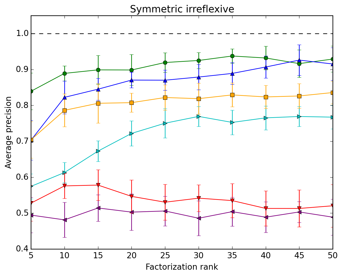
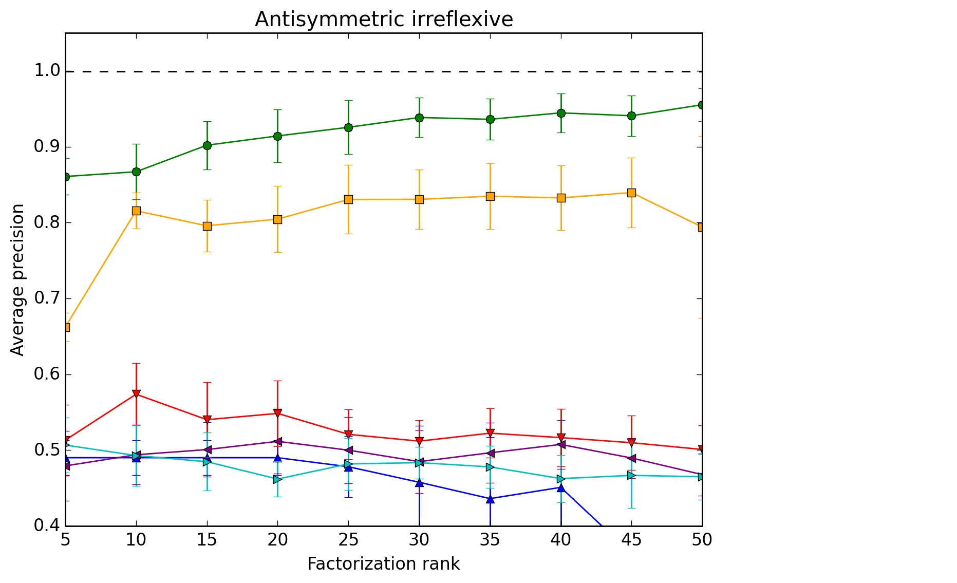
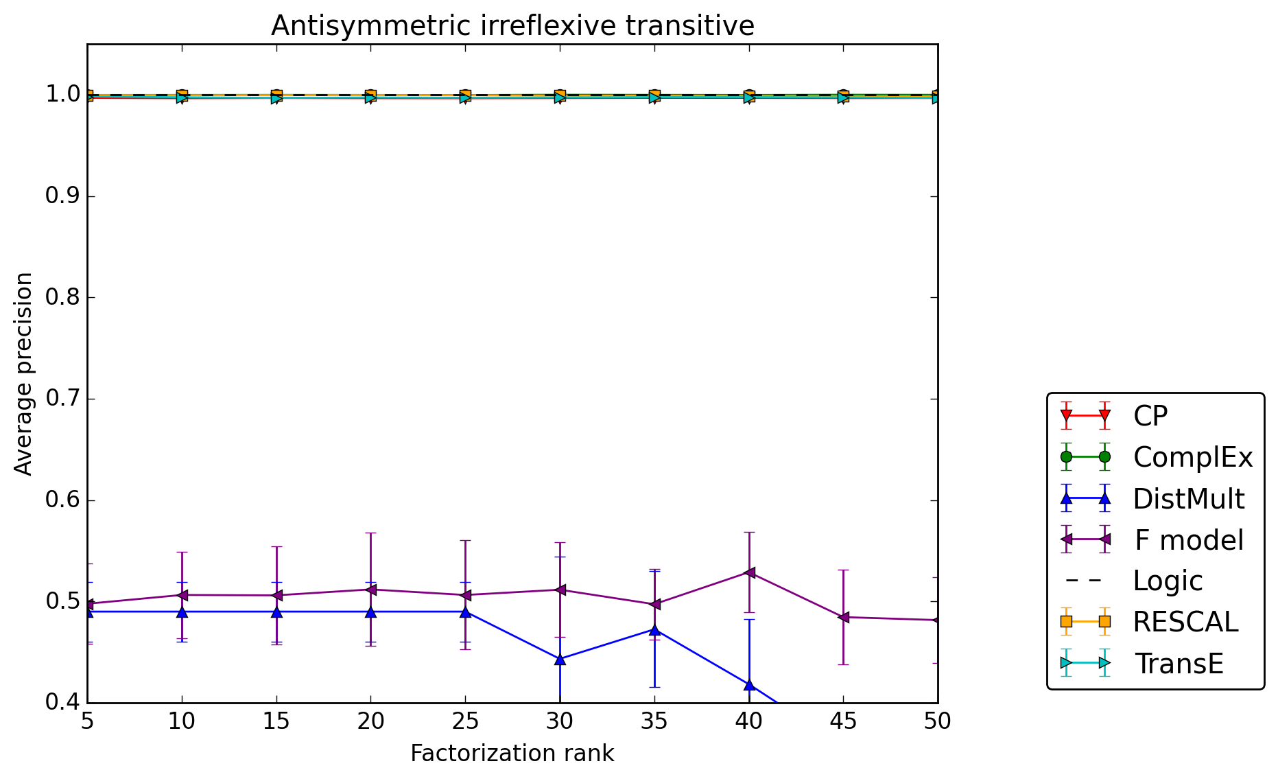
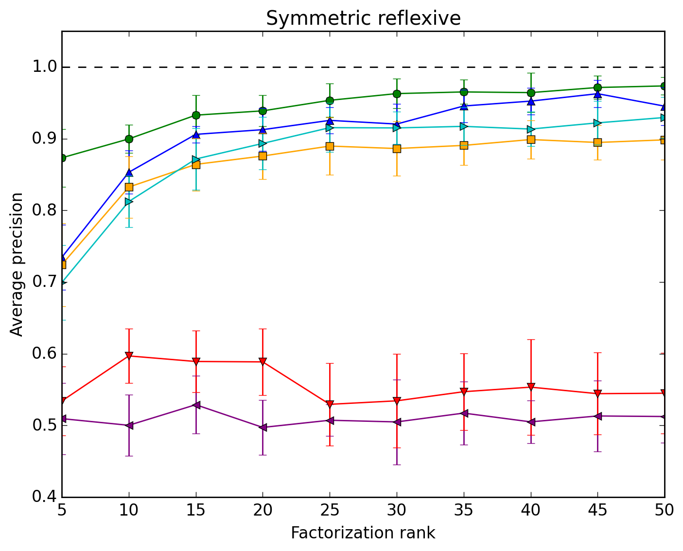
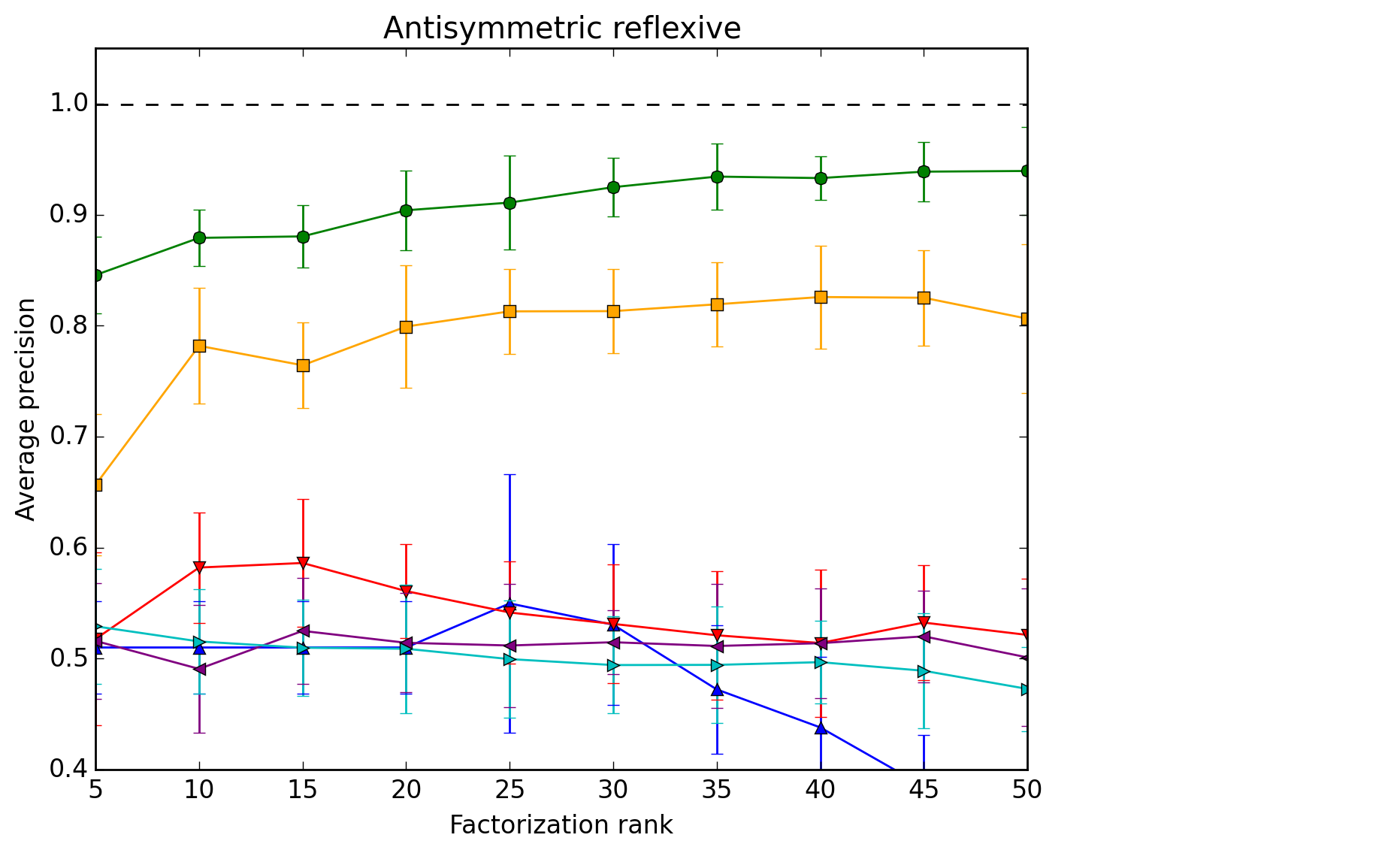
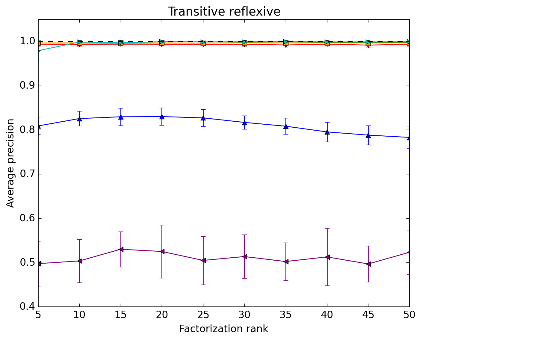
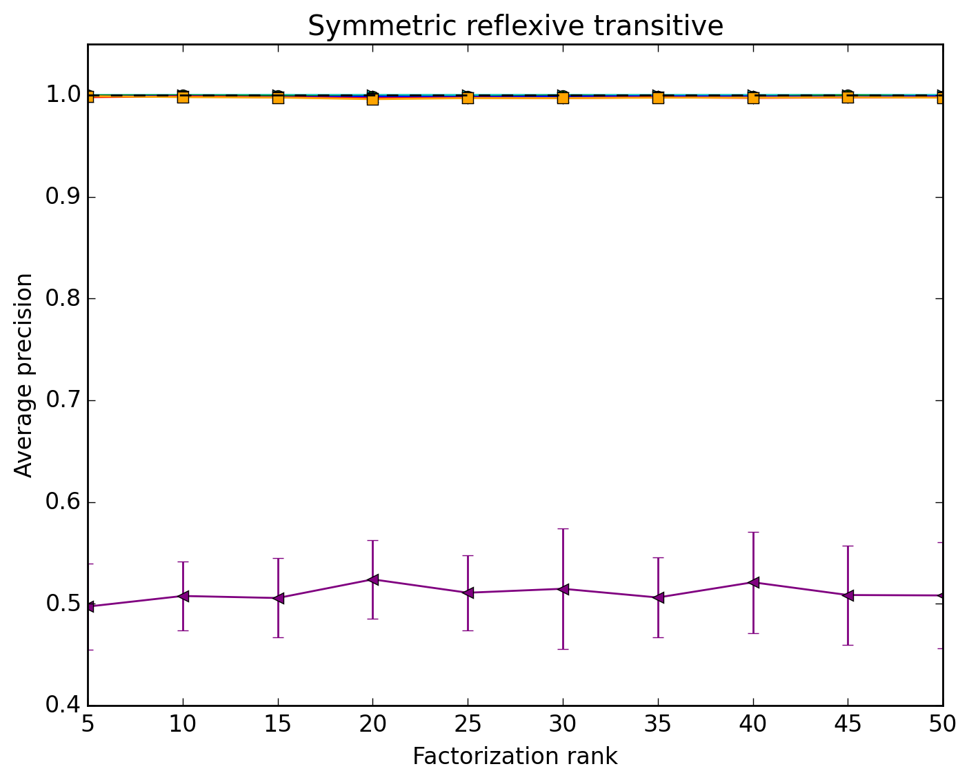
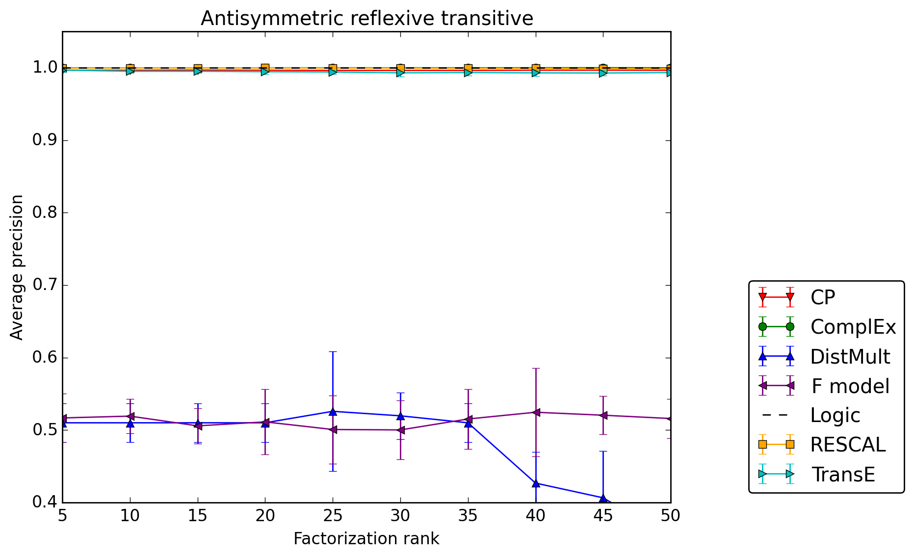
In this appendix we report results of the individual learning of combinations of relation properties including reflexivity and irreflexivity. Those results are included for completeness as they are similar to the cases that are neither reflexive nor irreflexive, reported in Section 4.2.1. Figure 12 shows results for the 5 combinations with reflexivity, and Figure 11 for the 3 combinations with irreflexivity. The irreflexive transitive case, and the irreflexive symmetric transitive case are not reported as they are not consistent, as explained in Section 4.1. The single noticeable difference is in the symmetric irreflexive case, where all models perform slightly worse compared to the symmetric and symmetric reflexive cases, especially TransE.

Figure 11: Generated irreflexive relations with 50 entities, combined with symmetry (top-left), antisymmetry (top-right) and antisymmetry and transitivity (bottom). Average precision for each rank ranging from 5 to 50 for each model.

Figure 12: Generated reflexive relations with 50 entities, combined with symmetry (top-left), antisymmetry (top-right), transitivity (middle), symmetry and transitivity (bottom-left) and antisymmetry and transitivity (bottom-right). Average precision for each rank ranging from 5 to 50 for each model.

References

- Aaronson, (2013) Aaronson, S. (2013). Why philosophers should care about computational complexity. In B. J. Copeland, C. P. and Shagrir, O., editors, Computability: Turing, Gödel, Church, and Beyond, pages 261–328. MIT Press.
- Alon et al., (2016) Alon, N., Moran, S., and Yehudayoff, A. (2016). Sign rank versus vc dimension. In Conference on Learning Theory, pages 47–80.
- Auer et al., (2007) Auer, S., Bizer, C., Kobilarov, G., Lehmann, J., and Ives, Z. (2007). DBpedia: A nucleus for a web of open data. In International Semantic Web Conference, Busan, Korea, pages 11–15. Springer.
- Bollacker et al., (2008) Bollacker, K., Evans, C., Paritosh, P., Sturge, T., and Taylor, J. (2008). Freebase: a collaboratively created graph database for structuring human knowledge. In ACM SIGMOD International Conference on Management of Data, pages 1247–1250.
- (5) Bordes, A., Usunier, N., Garcia-Duran, A., Weston, J., and Yakhnenko, O. (2013a). Irreflexive and hierarchical relations as translations. arXiv preprint arXiv:1304.7158.
- (6) Bordes, A., Usunier, N., Garcia-Duran, A., Weston, J., and Yakhnenko, O. (2013b). Translating embeddings for modeling multi-relational data. In Advances in Neural Information Processing Systems, pages 2787–2795.
- Bordes et al., (2011) Bordes, A., Weston, J., Collobert, R., and Bengio, Y. (2011). Learning structured embeddings of knowledge bases. In AAAI Conference on Artificial Intelligence.
- Bottou, (2014) Bottou, L. (2014). From machine learning to machine reasoning. Machine Learning, 94(2):133–149.
- Bouchard et al., (2015) Bouchard, G., Singh, S., and Trouillon, T. (2015). On approximate reasoning capabilities of low-rank vector spaces. AAAI Spring Symposium on Knowledge Representation and Reasoning: Integrating Symbolic and Neural Approaches.
- Bowman et al., (2015) Bowman, S. R., Potts, C., and Manning, C. D. (2015). Recursive neural networks can learn logical semantics. In ACL Workshop on Continuous Vector Space Models and their Compositionality.
- Cardano, (1545) Cardano, G. (1545). Artis Magnæ, Sive de Regulis Algebraicis Liber Unus.
- Caroll and Chang, (1970) Caroll, J. D. and Chang, J.-J. (1970). Analysis of individual differences in multidimensional scaling via -way generalization of Eckart–Young decomposition. Psychometrika, 35:283–319.
- Cyganiak et al., (2014) Cyganiak, R., Wood, D., and Lanthaler, M. (2014). RDF 1.1 concepts and abstract syntax. W3C Recommendation.
- Davis et al., (1993) Davis, R., Shrobe, H., and Szolovits, P. (1993). What is a knowledge representation? AI magazine, 14(1):17–33.
- Demeester et al., (2016) Demeester, T., Rocktäschel, T., and Riedel, S. (2016). Lifted rule injection for relation embeddings. In Empirical Methods in Natural Language Processing, pages 1389–1399.
- Dong et al., (2014) Dong, X., Gabrilovich, E., Heitz, G., Horn, W., Lao, N., Murphy, K., Strohmann, T., Sun, S., and Zhang, W. (2014). Knowledge vault: A web-scale approach to probabilistic knowledge fusion. In ACM SIGKDD International Conference on Knowledge Discovery and Data Mining, pages 601–610.
- Duchi et al., (2011) Duchi, J., Hazan, E., and Singer, Y. (2011). Adaptive subgradient methods for online learning and stochastic optimization. Journal of Machine Learning Research, 12:2121–2159.
- Dzeroski and Lavrac, (1994) Dzeroski, S. and Lavrac, N. (1994). Inductive logic programming: techniques and applications. Ellis Horwood, New York.
- Friedman et al., (1999) Friedman, N., Getoor, L., Koller, D., and Pfeffer, A. (1999). Learning probabilistic relational models. In International Joint Conference on Artificial Intelligence, volume 99, pages 1300–1309.
- Galárraga et al., (2015) Galárraga, L., Teflioudi, C., Hose, K., and Suchanek, F. M. (2015). Fast rule mining in ontological knowledge bases with amie+. The VLDB Journal, 24(6):707–730.
- García-Durán et al., (2014) García-Durán, A., Bordes, A., and Usunier, N. (2014). Effective blending of two and three-way interactions for modeling multi-relational data. In Joint European Conference on Machine Learning and Knowledge Discovery in Databases, pages 434–449. Springer.
- Getoor and Taskar, (2007) Getoor, L. and Taskar, B. (2007). Introduction to Statistical Relational Learning. MIT Press.
- Grefenstette, (2013) Grefenstette, E. (2013). Towards a formal distributional semantics: Simulating logical calculi with tensors. In Joint Conference on Lexical and Computational Semantics.
- Halmos, (1998) Halmos, P. R. (1998). Naive set theory. Springer Science & Business Media.
- Hamaguchi et al., (2017) Hamaguchi, T., Oiwa, H., Shimbo, M., and Matsumoto, Y. (2017). Knowledge transfer for out-of-knowledge-base entities: A graph neural network approach. arXiv preprint arXiv:1706.05674.
- Harshman, (1970) Harshman, R. A. (1970). Foundations of the PARAFAC procedure: models and conditions for an explanatory multimodal factor analysis. UCLA Working Papers in Phonetics, 16:1–84.
- Hayashi and Shimbo, (2017) Hayashi, K. and Shimbo, M. (2017). On the equivalence of holographic and complex embeddings for link prediction. arXiv preprint arXiv:1702.05563.
- Heckerman et al., (2007) Heckerman, D., Meek, C., and Koller, D. (2007). Probabilistic entity-relationship models, prms, and plate models. Introduction to statistical relational learning, pages 201–238.
- Hinton, (1986) Hinton, G. E. (1986). Learning distributed representation of concepts. In Conference of the Cognitive Science Society.
- Hitchcock, (1927) Hitchcock, F. L. (1927). The expression of a tensor or a polyadic as a sum of products. Journal of Mathematical Physics, 6(1):164–189.
- Jenatton et al., (2012) Jenatton, R., Bordes, A., Le Roux, N., and Obozinski, G. (2012). A latent factor model for highly multi-relational data. In Advances in Neural Information Processing Systems, pages 3167–3175.
- Kearns and Valiant, (1994) Kearns, M. and Valiant, L. (1994). Cryptographic limitations on learning boolean formulae and finite automata. Journal of the ACM, 41(1):67–95.
- Kersting and De Raedt, (2001) Kersting, K. and De Raedt, L. (2001). Towards combining inductive logic programming with bayesian networks. In International Conference on Inductive Logic Programming, pages 118–131.
- Koren, (2008) Koren, Y. (2008). Factorization meets the neighborhood: A multifaceted collaborative filtering model. In ACM SIGKDD International Conference on Knowledge Discovery and Data Mining, pages 426–434.
- Koren et al., (2009) Koren, Y., Bell, R., and Volinsky, C. (2009). Matrix factorization techniques for recommender systems. Computer, 42(8):30–37.
- Lewis and Steedman, (2013) Lewis, M. and Steedman, M. (2013). Combining distributional and logical semantics. Transactions of the Association for Computational Linguistics, 1:179–192.
- Linial et al., (2007) Linial, N., Mendelson, S., Schechtman, G., and Shraibman, A. (2007). Complexity measures of sign matrices. Combinatorica, 27(4):439–463.
- Lisi, (2010) Lisi, F. A. (2010). Inductive logic programming in databases: From datalog to. Theory and Practice of Logic Programming, 10(3):331–359.
- Ma et al., (2015) Ma, Y., Crook, P. A., Sarikaya, R., and Fosler-Lussier, E. (2015). Knowledge graph inference for spoken dialog systems. In IEEE International Conference on Acoustics, Speech and Signal Processing, pages 5346–5350.
- Minervini et al., (2017) Minervini, P., Demeester, T., Rocktäschel, T., and Riedel, S. (2017). Adversarial sets for regularising neural link predictors. In Conference on Uncertainty in Artificial Intelligence.
- Muggleton, (1995) Muggleton, S. (1995). Inverse entailment and progol. New generation computing, 13(3-4):245–286.
- Muggleton and De Raedt, (1994) Muggleton, S. and De Raedt, L. (1994). Inductive logic programming: Theory and methods. The Journal of Logic Programming, 19:629–679.
- Ngo and Haddawy, (1997) Ngo, L. and Haddawy, P. (1997). Answering queries from context-sensitive probabilistic knowledge bases. Theoretical Computer Science, 171(1):147–177.
- (44) Nickel, M., Murphy, K., Tresp, V., and Gabrilovich, E. (2016a). A review of relational machine learning for knowledge graphs. Proceedings of the IEEE, 104(1):11–33.
- (45) Nickel, M., Rosasco, L., and Poggio, T. A. (2016b). Holographic embeddings of knowledge graphs. In AAAI Conference on Artificial Intelligence, pages 1955–1961.
- Nickel and Tresp, (2013) Nickel, M. and Tresp, V. (2013). Logistic tensor factorization for multi-relational data. arXiv preprint arXiv:1306.2084.
- Nickel et al., (2011) Nickel, M., Tresp, V., and Kriegel, H.-P. (2011). A three-way model for collective learning on multi-relational data. In International Conference on Machine Learning, pages 809–816.
- Popper, (1934) Popper, K. (1934). Logik der Forschung. Mohr Siebeck.
- Richardson and Domingos, (2006) Richardson, M. and Domingos, P. (2006). Markov logic networks. Machine Learning, 62(1-2):107–136.
- Riedel et al., (2013) Riedel, S., Yao, L., McCallum, A., and Marlin, B. M. (2013). Relation extraction with matrix factorization and universal schemas. In North American Chapter of the Association of Computational Linguistics: Human Language Technologies, pages 74–84.
- Rocktäschel et al., (2014) Rocktäschel, T., Bosnjak, M., Singh, S., and Riedel, S. (2014). Low-dimensional embeddings of logic. In Workshop on semantic parsing at ACL.
- Rocktäschel and Riedel, (2016) Rocktäschel, T. and Riedel, S. (2016). Learning knowledge base inference with neural theorem provers. Workshop on Automated Knowledge Base Construction at NAACL-HLT, pages 45–50.
- Rocktäschel et al., (2015) Rocktäschel, T., Singh, S., and Riedel, S. (2015). Injecting logical background knowledge into embeddings for relation extraction. In North American Chapter of the Association for Computational Linguistics: Human Language Technologies, pages 1119–1129.
- Singh et al., (2015) Singh, S., Rocktäschel, T., and Riedel, S. (2015). Towards combined matrix and tensor factorization for universal schema relation extraction. In Workshop on Vector Space Modeling for Natural Language Processing at NAACL-HLT, pages 135–142.
- Smolensky et al., (2016) Smolensky, P., Lee, M., He, X., Yih, W.-t., Gao, J., and Deng, L. (2016). Basic reasoning with tensor product representations. arXiv preprint arXiv:1601.02745.
- Socher et al., (2013) Socher, R., Chen, D., Manning, C. D., and Ng, A. (2013). Reasoning with neural tensor networks for knowledge base completion. In Advances in Neural Information Processing Systems, pages 926–934.
- Sutskever et al., (2009) Sutskever, I., Tenenbaum, J. B., and Salakhutdinov, R. R. (2009). Modelling relational data using bayesian clustered tensor factorization. In Advances in neural information processing systems, pages 1821–1828.
- Trouillon et al., (2017) Trouillon, T., Dance, C. R., Welbl, J., Riedel, S., Gaussier, É., and Bouchard, G. (2017). Knowledge graph completion via complex tensor factorization. arXiv preprint arXiv:1702.06879. To appear in the Journal of Machine Learning Research.
- Trouillon and Nickel, (2017) Trouillon, T. and Nickel, M. (2017). Complex and holographic embeddings of knowledge graphs: a comparison. International Workshop on Statistical Relational AI.
- Trouillon et al., (2016) Trouillon, T., Welbl, J., Riedel, S., Gaussier, E., and Bouchard, G. (2016). Complex embeddings for simple link prediction. In International Conference on Machine Learning, volume 48, pages 2071–2080.
- Valiant, (1984) Valiant, L. G. (1984). A theory of the learnable. Communications of the ACM, 27(11):1134–1142.
- Vapnik, (1995) Vapnik, V. N. (1995). The Nature of Statistical Learning Theory. Springer-Verlag New York, Inc.
- Verga et al., (2017) Verga, P., Neelakantan, A., and McCallum, A. (2017). Generalizing to unseen entities and entity pairs with row-less universal schema. In European Chapter of the Association of Computational Linguistics.
- Wang and Cohen, (2016) Wang, W. Y. and Cohen, W. W. (2016). Learning first-order logic embeddings via matrix factorization. In International Joint Conference on Artificial Intelligence, pages 2132–2138.
- Welbl et al., (2016) Welbl, J., Bouchard, G., and Riedel, S. (2016). A factorization machine framework for testing bigram embeddings in knowledge base completion. In Workshop on Automated Knowledge Base Construction at NAACL-HLT, pages 103–107.
- Wellman et al., (1992) Wellman, M. P., Breese, J. S., and Goldman, R. P. (1992). From knowledge bases to decision models. The Knowledge Engineering Review, 7(01):35–53.
- Weston et al., (2015) Weston, J., Bordes, A., Chopra, S., Rush, A. M., van Merriënboer, B., Joulin, A., and Mikolov, T. (2015). Towards AI-complete question answering: A set of prerequisite toy tasks. arXiv preprint arXiv:1502.05698.
- Wikipedia, (2004) Wikipedia (2004). Binary relation — Wikipedia, the free encyclopedia. https://en.wikipedia.org/wiki/Binary_relation.
- Yang et al., (2015) Yang, B., Yih, W.-t., He, X., Gao, J., and Deng, L. (2015). Embedding entities and relations for learning and inference in knowledge bases. In International Conference on Learning Representations.
- Yoon et al., (2016) Yoon, H.-G., Song, H.-J., Park, S.-B., and Park, S.-Y. (2016). A translation-based knowledge graph embedding preserving logical property of relations. In North American Chapter of the Association of Computational Linguistics: Human Language Technologies, pages 907–916.