Millimeter Wave Channel Measurements and Implications for PHY Layer Design

Abstract

There has been an increasing interest in the millimeter wave (mmW) frequency regime in the design of next-generation wireless systems. The focus of this work is on understanding mmW channel properties that have an important bearing on the feasibility of mmW systems in practice and have a significant impact on physical (PHY) layer design. In this direction, simultaneous channel sounding measurements at $2.9$, $29$ and $61$ GHz are performed at a number of transmit-receive location pairs in indoor office, shopping mall and outdoor environments. Based on these measurements, this paper first studies large-scale properties such as path loss and delay spread across different carrier frequencies in these scenarios. Towards the goal of understanding the feasibility of outdoor-to-indoor coverage, material measurements corresponding to mmW reflection and penetration are studied and significant notches in signal reception spread over a few GHz are reported. Finally, implications of these measurements on system design are discussed and multiple solutions are proposed to overcome these impairments.

I Introduction

Recent attention on millimeter wave (mmW) systems for meeting the high data-rate demands in next-generation devices has resulted in a burgeoning interest in the focus on these systems [2, 3, 4, 5]. Given the unfavorable wireless propagation in mmW settings [6, 7], it is now understood that physical (PHY) layer system design has to consider innovative approaches to address these impairments. In particular, beamforming with a large number of antennas [8, 9, 10, 11, 12, 13, 14, 15, 16] is a key ingredient in meeting the link margin of mmW systems. Towards the goal of realizing beamforming-based mmW systems, there has been a strong interest in understanding radio frequency (RF) design challenges for large bandwidth systems [17, 18, 19], as well as measurements and channel modeling at different carrier frequencies of interest. In particular, there have been multiple studies in the modeling of $60$ GHz indoor channels [20, 21, 22], as well as channels at other carrier frequencies such as $15$ GHz [23], $28$ GHz [24, 25, 26], $38$-$39$ GHz [27], $73$ GHz [28], etc.

The scope of this work is on further understanding some of the representative large-scale mmW channel characteristics, additional impairments encountered in practical implementations of these systems, and the implications these observations have on PHY layer design.

Towards this goal, we start with channel propagation comparisons based on measurements at the same transmit-receive location pairs at $2.9$, $29$ and $61$ GHz in the indoor office, shopping mall and outdoor environments. In addition to the vast set of measurements in different settings reported here, this work makes an important and novel contribution given the fact that most papers in the mmW literature consider channel measurements at individual mmW frequencies and not at the same location pairs. Such a study allows us to legitimately compare propagation at different frequencies. Our studies show that losses at mmW frequencies are typically higher than with sub-$6$ GHz systems in both indoor and outdoor settings. However, these losses are not significantly worse at the mmW regime relative to sub-$6$ GHz settings. While the observed delay spreads are typically small in indoor settings, outdoor settings can lead to significant increases in delay spreads corresponding to strong reflections from distant objects. Beamformed delay spreads are expected to be smaller than omni delay spreads in most scenarios.

Building on these studies, we then branch off into impairments arising from specific practical implementations. Given that indoor WiFi replacement is an important use-case of mmW systems and actively considered by the 5GTF (${\tt www.5gtf.org}$), we then study the impact of reflection response and penetration through walls of residential buildings. Our studies show that significant loss of coverage can be observed at mmW frequencies corresponding to deep frequency notches which needs to be overcome with adequate spatial and frequency diversity. We also report that at mmW frequencies, the penetration depth of electromagnetic (EM) energy into the human body is small and a significant fraction of the energy is reflected. This observation is of particular importance in stadium deployments.

This paper is organized as follows. Section II provides a brief overview of the channel sounder, measurement methodology and measurement scenarios. Section III studies large-scale channel parameters such as path loss and delay spreads in indoor and outdoor environments. Section IV reports reflection response and penetration loss characterization with materials commonly found in residential and indoor environments. Section V illustrates the impact on PHY layer of all the observations from Secs. III-IV and Section VI concludes the paper.

II Measurement Setup and Methodology

II-A Channel Sounder

We begin with a brief description of the channel sounder and measurement methodology. Measurements were performed with a battery-powered and freely-mobile channel sounder that allows automatic omni-directional scans at $2.9$, $29$ and $61$ GHz, and elevation and azimuthal scans at $29$ and $61$ GHz. Parallel data-sets for these frequencies were obtained at identical transmit and receive locations using omni-directional antennas without swapping cables. In addition, directional horn antennas with $10$ and $20$ dBi gains were used to obtain measurements at $29$ and $61$ GHz. Directional scans consisted of azimuthal ($360^{\sf o}$ view) and spherical scans ($360^{\sf o}$ azimuth view and $-30^{\sf o}$ to $90^{\sf o}$ view in elevation). The resultant scans included $39$ slices with a $10$ dBi gain antenna and $331$ slices with a $20$ dBi gain antenna. The resolution of the channel sounder is approximately $5$ ns. An Agilent E8267D signal generator is used to generate a pseudo-noise (PN) sequence at a chip rate of $100$ Mc/s, which is then used to sound the channel. At the receiver, an Agilent N9030A signal analyzer is used for acquisition and the PN chip sequence is despread using a sampler at $200$ MHz and with $16$ bit resolution.

The omni-directional antennas allow us to measure path loss variations up to $180$ dB. Thus, in understanding macroscopic channel properties (such as path loss and delay spread), we do not need to obtain the omni-directional channel response by stitching together directional/horn responses. However, our measurements are constructed out of a variable-time integration of omni-directional responses to ensure that there is sufficient signal strength to allow signal discrimination. This variable time could be anywhere from less than $1$ ms to a few tens of ms, depending on the link margin/distance between transmitter and receiver. Up to $80$ dB processing gain is realized in the channel acquisition process.

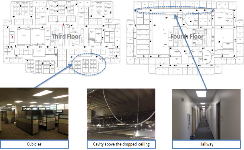
Figure 1: Indoor layout across the third and fourth floor of the Qualcomm building. Transmitter and receiver locations are marked in red and black circles, respectively.

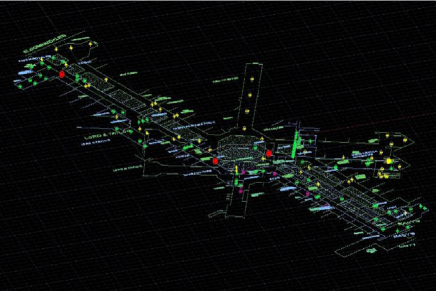
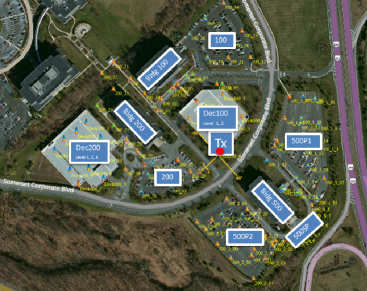
(a)	(b)

Figure 2: (a) Shopping mall layout with transmitter and receiver locations in red and green/yellow circles. (b) Measurement layout outside the Qualcomm building in Bridgewater, NJ.

II-B Measurement Locations

Indoor office measurements were made across two floors of the Qualcomm building in Bridgewater, NJ, USA, with dimensions of $75\times 40\times 2.68$ m³. The building construction is representative of a modern office building in the USA. See Fig. 1 for more details on the office layout across the two floors and measurement locations (transmitter in red and receiver in black).

The two floors represent two types of typical office environments. The third floor is mostly comprised of cubicles along the edge of the floor plan with walled offices and conference rooms towards the center. The fourth floor is comprised of walled offices (larger than the third floor), conference rooms and laboratories. The partition walls are constructed with metallic studs spaced at $0.46$ m ($1.5$ ft) intervals. The ceiling is a dropped ceiling $2.7$ m ($\sim{}9$ ft) above the floor with an additional $0.91$ m ($\sim{}3$ ft) cavity below the concrete ceiling. While the cavity is not a visible aspect of the office, the abundance of metal objects such as concrete ceiling with a corrugated metal substrate and metal duct-work pipes in a fairly open space plays an important role in propagation measurements. On the third floor, the measurements were made between two transmitter locations and the same set of multiple receiver locations. The first transmitter location is centrally located, while the second one is positioned at the left-hand edge of the floor plan. On the fourth floor, the measurements were made between a single transmitter location and multiple receiver locations. Given the high density of partition walls in the office building, a large majority of the measurements were non-line-of-sight (NLOS) in nature.

Indoor shopping mall measurements were made at the Bridgewater Commons Mall, Bridgewater, NJ, USA, which is a large three level indoor shopping mall with an open interior design. The mall layout as well as the measurement locations are seen in Fig. 2(a). The building length is $\sim{}390$ m with the longest testing range of $\sim{}275$ m. Measurements were obtained at three transmitter and multiple receiver locations (on all the three levels of the mall). The transmitter locations were: i) centrally located on the second floor, ii) located on an edge of the second floor, and iii) centrally located on the third floor near an open-area food court. Multi-floor propagation was also studied. The specific design of the mall leads to the observation of a number of both line-of-sight (LOS) and NLOS links.

The first set of outdoor measurements were obtained in downtown New Brunswick, NJ corresponding to an Urban Micro (UMi)-type environment. Measurements were obtained from one transmitter location (antenna height of $6.5$ m) and multiple receiver locations (all at a height of $1.5$ m). The second set of outdoor measurements were obtained outside the Qualcomm building and around Somerset Corporate Boulevard in Bridgewater, NJ (see layout in Fig. 2(b)). The measurement site is mostly a tree-lined open square-type setting with some street canyon-type environment. Specific points of interest include parking lots and structures with bordering buildings, vegetation which is a mix of pine and spruce trees, and a large shopping mall in close vicinity (Bridgewater Commons Mall). Highways (US Rt. $22$ and I-$287$) are in close proximity with occasional reflections from vehicles in a number of measurement scenarios. The measurements were made from a single transmitter location and multiple receiver locations from within $10$ points-of-interest, with transmit-receive link distances ranging from $35$-$256$ m. Of particular interest are links corresponding to open areas and parking structures.

Some indoor office measurements were obtained over regular day-time office hours and some were obtained over non-office hours. Due to logistical constraints, shopping mall measurements were conducted over the night-time with minimal footfall and in common areas with no inside store access. Tests in downtown New Brunswick were performed during the day-time with a heavy pedestrian and vehicular traffic in the measurement areas. Measurements outside the Qualcomm building were done during the day-time with sporadic (and mostly) vehicular traffic in the neighborhood. Our measurements do not indicate a significant impact of humans or vehicles on macroscopic metrics such as path loss and delay spread. This is because our measurements were repeated $5$ times at the same location to average over dynamic influences. Each receiver location was measured at five separate locations offset from each other (center of a circle with a radius of $18$ cm along with $4$ points on the circumference) to get diversity in measurements and to avoid possible nulls in the channel response. The correlation over the temporal measurements was high (over $90\%$) indicating that the scale at which humans move did not have a substantial effect on the macroscopic channel properties.

III Large-Scale Channel Properties

TABLE I: Path Loss Coefficients for the Different Indoor Settings. $f_{\sf c}$ is in GHz, $\sigma_{\sf CI},\sigma_{\sf ABG},\beta^{\prime}$ are in ${\rm dB}$.

${\bf{\hskip 36.135pt}Indoor\hskip 3.61371ptOffice}$
		${\sf LOS}$						${\sf NLOS}$
	$f_{\sf c}$	${\sf No.meas.}$	${\sf PLE}$	$\sigma_{\sf CI}$	$\alpha$	$\beta^{\prime}$	$\sigma_{\sf ABG}$	${\sf No.meas.}$	${\sf PLE}$	$\sigma_{\sf CI}$	$\alpha$	$\beta^{\prime}$	$\sigma_{\sf ABG}$
All	$2.9$	$17$	$1.62$	$5.49$	$2.11$	$35.47$	$5.28$	$105$	$3.08$	$6.60$	$4.36$	$23.08$	$5.81$
	$29$	$17$	$1.46$	$4.25$	$1.48$	$61.36$	$4.25$	$106$	$3.46$	$8.31$	$4.96$	$39.79$	$7.45$
	$61$	$19$	$1.59$	$4.81$	$1.03$	$75.47$	$4.50$	$279$	$4.17$	$13.83$	$4.23$	$67.18$	$13.83$
Tx 1	$2.9$	$2$	$2.20$	$1.25$	$-$	$-$	$-$	$38$	$3.20$	$7.87$	$4.49$	$22.25$	$6.81$
	$29$	$1$	$1.84$	$0$	$-$	$-$	$-$	$34$	$3.64$	$10.27$	$5.24$	$37.68$	$8.74$
	$61$	$2$	$2.82$	$1.26$	$-$	$-$	$-$	$40$	$4.15$	$18.06$	$5.20$	$52.13$	$17.82$
Tx 2	$2.9$	$4$	$2.08$	$3.96$	$3.05$	$28.12$	$3.56$	$33$	$3.03$	$4.81$	$4.63$	$19.71$	$3.86$
	$29$	$5$	$1.71$	$5.83$	$3.99$	$30.61$	$4.06$	$39$	$3.46$	$6.23$	$5.49$	$33.40$	$5.17$
Tx 3	$2.9$	$11$	$1.35$	$2.95$	$2.03$	$48.04$	$1.96$	$34$	$2.98$	$6.22$	$3.90$	$28.11$	$5.91$
	$29$	$11$	$1.30$	$1.84$	$1.03$	$65.11$	$1.62$	$33$	$3.26$	$7.41$	$4.08$	$49.61$	$7.23$
	$61$	$17$	$1.54$	$3.88$	$1.63$	$66.94$	$3.87$	$239$	$4.17$	$13.03$	$3.86$	$73.00$	$13.02$
${\bf{\hskip 36.135pt}Shopping\hskip 3.61371ptMall}$
		${\sf LOS}$						${\sf NLOS}$
	$f_{\sf c}$	${\sf No.meas.}$	${\sf PLE}$	$\sigma_{\sf CI}$	$\alpha$	$\beta^{\prime}$	$\sigma_{\sf ABG}$	${\sf No.meas.}$	${\sf PLE}$	$\sigma_{\sf CI}$	$\alpha$	$\beta^{\prime}$	$\sigma_{\sf ABG}$
All	$2.9$	$29$	$1.93$	$5.32$	$1.74$	$45.09$	$5.29$	$151$	$2.61$	$9.08$	$2.81$	$37.61$	$9.07$
	$29$	$26$	$1.98$	$3.56$	$1.62$	$68.43$	$3.45$	$132$	$2.76$	$9.47$	$2.96$	$57.57$	$9.45$
	$61$	$25$	$2.05$	$4.29$	$1.90$	$70.86$	$4.27$	$132$	$2.98$	$12.86$	$2.27$	$82.05$	$12.70$
Tx 1	$2.9$	$12$	$1.97$	$7.04$	$1.85$	$43.70$	$7.03$	$82$	$2.64$	$9.85$	$2.19$	$50.31$	$9.80$
	$29$	$8$	$1.94$	$1.67$	$1.86$	$63.06$	$1.66$	$61$	$2.78$	$10.87$	$1.42$	$87.44$	$10.46$
	$61$	$8$	$1.94$	$1.30$	$1.69$	$72.40$	$1.03$	$58$	$2.97$	$12.53$	$1.43$	$97.28$	$12.07$
Tx 2	$2.9$	$8$	$1.79$	$3.04$	$3.59$	$5.75$	$1.91$	$38$	$2.72$	$5.89$	$3.07$	$34.29$	$5.78$
	$29$	$9$	$1.86$	$2.96$	$2.96$	$39.69$	$2.60$	$44$	$2.88$	$7.38$	$3.63$	$45.60$	$7.04$
	$61$	$8$	$1.97$	$5.06$	$3.86$	$30.51$	$4.41$	$42$	$3.21$	$11.72$	$2.05$	$92.46$	$10.83$
Tx 3	$2.9$	$9$	$2.03$	$3.33$	$2.62$	$31.07$	$3.21$	$31$	$2.35$	$8.61$	$2.75$	$33.96$	$8.56$
	$29$	$9$	$2.16$	$3.19$	$1.14$	$79.86$	$2.80$	$27$	$2.46$	$6.65$	$3.03$	$50.86$	$6.52$
	$61$	$9$	$2.22$	$3.93$	$1.77$	$76.03$	$3.87$	$32$	$2.65$	$12.46$	$2.35$	$73.89$	$12.44$

TABLE II: Path Loss Coefficients for the Different Outdoor Settings. $f_{\sf c}$ is in GHz, $\sigma_{\sf CI},\sigma_{\sf ABG},\beta^{\prime}$ are in ${\rm dB}$.

${\bf{\hskip 36.135pt}UMi,\hskip 3.61371ptStreet\hskip 3.61371ptCanyon}$
		${\sf LOS}$						${\sf NLOS}$
	$f_{\sf c}$	${\sf No.meas.}$	${\sf PLE}$	$\sigma_{\sf CI}$	$\alpha$	$\beta^{\prime}$	$\sigma_{\sf ABG}$	${\sf No.meas.}$	${\sf PLE}$	$\sigma_{\sf CI}$	$\alpha$	$\beta^{\prime}$	$\sigma_{\sf ABG}$
All	$2.9$	$6$	$2.18$	$4.41$	$3.23$	$18.87$	$3.35$	$35$	$2.95$	$7.82$	$4.32$	$12.50$	$7.60$
	$29$	$7$	$2.19$	$4.37$	$3.11$	$42.31$	$3.47$	$41$	$3.07$	$8.16$	$4.40$	$33.39$	$7.97$
	$61$	$6$	$2.22$	$4.84$	$3.12$	$48.91$	$4.19$	$40$	$3.27$	$10.70$	$5.18$	$27.56$	$10.41$
${\bf{\hskip 36.135pt}Outside\hskip 3.61371ptQualcomm\hskip 3.61371ptBuilding,\hskip 3.61371ptOpen\hskip 3.61371ptAreas}$
		${\sf LOS}$						${\sf NLOS}$
	$f_{\sf c}$	${\sf No.meas.}$	${\sf PLE}$	$\sigma_{\sf CI}$	$\alpha$	$\beta^{\prime}$	$\sigma_{\sf ABG}$	${\sf No.meas.}$	${\sf PLE}$	$\sigma_{\sf CI}$	$\alpha$	$\beta^{\prime}$	$\sigma_{\sf ABG}$
All	$2.9$	$47$	$2.41$	$4.60$	$3.03$	$28.54$	$4.56$	$13$	$3.01$	$4.00$	$5.91$	$-21.29$	$3.07$
	$29$	$49$	$2.73$	$5.73$	$2.46$	$67.31$	$5.72$	$13$	$3.39$	$8.03$	$8.70$	$-53.36$	$6.53$
	$61$	$37$	$2.83$	$6.78$	$5.40$	$13.38$	$6.24$	$6$	$3.42$	$1.97$	$0.08$	$137.81$	$0.83$
${\bf{\hskip 36.135pt}Outside\hskip 3.61371ptQualcomm\hskip 3.61371ptBuilding,\hskip 3.61371ptParking\hskip 3.61371ptStructures}$
		${\sf LOS}$						${\sf NLOS}$
	$f_{\sf c}$	${\sf No.meas.}$	${\sf PLE}$	$\sigma_{\sf CI}$	$\alpha$	$\beta^{\prime}$	$\sigma_{\sf ABG}$	${\sf No.meas.}$	${\sf PLE}$	$\sigma_{\sf CI}$	$\alpha$	$\beta^{\prime}$	$\sigma_{\sf ABG}$
All	$2.9$	$10$	$2.82$	$13.54$	$0.82$	$83.95$	$8.26$	$35$	$3.23$	$8.54$	$2.85$	$49.94$	$8.44$
	$29$	$9$	$2.94$	$21.02$	$-0.49$	$132.71$	$9.57$	$36$	$3.44$	$10.50$	$2.21$	$88.41$	$9.63$

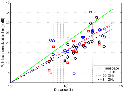
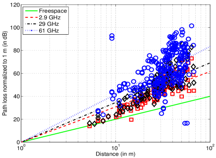
(a)	(b)
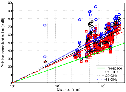
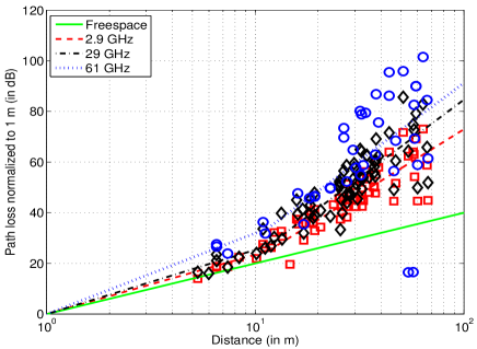
(c)	(d)

Figure 3: Path loss fits with the CI model for (a) LOS and (b) NLOS links for indoor office, and (c) with NLOS links for shopping mall settings. (d) Dual-slope model for NLOS links in third floor of indoor office.

III-A Path Loss

The total received power from omni-directional antenna measurements is used to estimate the path loss model for $2.9$, $29$ and $61$ GHz. The path loss from measurements is fitted with two popular frequency-dependent models in the literature [6]: the close-in (CI) reference model and the Alpha-Beta-Gamma (ABG) model. In the CI model, the path loss at a distance of $d$ m is given as

$${\sf PL}(d)={\sf PL}(d_{0})+{\sf PLE}\cdot 10\log_{10}(d/d_{0})+X_{\sf CI}\hskip 7.22743pt\hskip 7.22743pt[{\sf in\hskip 3.61371ptdB}]$$ (1)

where ${\sf PL}(d_{0})$ is the path loss at a reference distance of $d_{0}$ m, ${\sf PLE}$ is the path loss exponent (PLE), and $X_{\sf CI}\sim{\cal N}(0,\sigma_{\sf CI}^{2})$ models log-normal shadowing. With the reference distance typically set to $d_{0}=1$ m, the reference path loss ${\sf PL}(d_{0})=20\cdot\log_{10}\left(\frac{4\pi d_{0}}{\lambda}\right)$ is removed from the measurement data to normalize the path loss to $0$ dB at $d_{0}$ for all the three frequencies thus allowing a direct comparison. An estimate of the PLE and $\sigma_{\sf CI}$ are obtained through a least-squares fit of the parameters to the measurement data.

In the ABG model, the path loss is given as

$${\sf PL}(d) = 10\alpha\cdot\log_{10}\left(\frac{d}{d_{0}}\right)+\underbrace{\beta+10\gamma\cdot\log_{10}\left(\frac{f_{\sf c}}{1\hskip 1.4457pt{\sf GHz}}\right)}_{=\beta^{\prime}}$$ (2)

$${\hskip 14.45377pt}+X_{\sf ABG}\hskip 7.22743pt\hskip 7.22743pt[{\sf in\hskip 3.61371ptdB}]$$

where $\alpha$ and $\gamma$ capture how the path loss changes with distance and frequency, $\beta$ is an optimized parameter and $X_{\sf ABG}\sim{\cal N}(0,\sigma_{\sf ABG}^{2})$ models log-normal shadowing. The CI and ABG models trade off explanatory power at the cost of more model parameters (better fit with the four parameter ABG model). As in the CI case, the model parameters in the ABG case are also learned using a least-squares fit of the parameters to measurement data. Tables I and II present the parameters for the CI and ABG models in both LOS and NLOS settings at different carrier frequencies and measurement scenarios. Table I focusses on the indoor scenario (office and mall), whereas Table II focusses on the outdoor scenario (downtown New Brunswick and outside Qualcomm building). Figs. 3(a)-(c) present the path loss fits with the CI model in the office and mall settings.

In the indoor office setting, both third and fourth floor data were combined together in obtaining a global estimate of PLE and shadowing factors with both models across the building. The best fit PLEs and shadowing factors for NLOS links at $2.9$, $29$ and $61$ GHz are $3.1$, $3.5$ and $4.2$, and $6.6$, $8.3$ and $13.8$ dB, respectively. On the other hand, path loss fits conditioned on third floor locations alone suggest a better fit with a dual-slope model corresponding to a breakpoint distance of ${d}_{\sf BP}$ than a single-slope model:

$${\sf PL}(d)-{\sf PL}(d_{0})$$

$$=\left\{\begin{array}[]{l}{\sf PLE}_{1}\cdot 10\log_{10}(d/d_{0})+X_{\sf CI}^{1}\hskip 3.61371pt{\sf if}\hskip 3.61371ptd<{d}_{\sf BP}\\ {\sf PLE}_{2}\cdot 10\log_{10}(d/{d}_{\sf BP})+{\sf PLE}_{1}\cdot 10\log_{10}({d}_{\sf BP})+X_{\sf CI}^{2}\\ {\hskip 173.44756pt}\hskip 3.61371pt{\sf if}\hskip 3.61371ptd\geq{d}_{\sf BP}\end{array}\right.$$ (6)

For example, at $2.9$ GHz, we obtain $d_{\sf BP}=11.5$ m, ${\sf PLE}_{1}=2.35$, ${\sf PLE}_{2}=5.12$, $\sigma_{\sf CI}^{1}=2.03$ dB, $\sigma_{\sf CI}^{2}=5.98$ dB leading to a net shadowing factor of $5.68$ dB. On the other hand, the single slope model results in ${\sf PLE}=3.13$ and $\sigma_{\sf CI}=6.69$ dB. The path loss fits in the NLOS setting at different frequencies are presented in Fig. 3(d). These observations suggest that two distinct modes of communications may be possible in indoor settings (long walkways and office rooms in fourth floor vs. primarily cubicles and conference rooms in third floor): predominantly reflected and diffracted paths at $d<d_{\sf BP}$ and $d\geq d_{\sf BP}$, respectively. PLEs for LOS links in the indoor office setting are considerably lower: $1.6$, $1.5$ and $1.6$ at $2.9$, $29$ and $61$ GHz, respectively. The discrepancy of lower PLE at $29$ GHz is ascribed to waveguide effects in the indoor office setting and/or changes in material properties at higher frequencies. The $\beta^{\prime}$ parameter estimated with the ABG model shows wide variations, also documented in other works such as [32].

In the mall use-case with NLOS links, the PLEs and $\sigma_{\sf CI}$ at these three frequencies are $2.6$, $2.8$ and $3.0$, and $9.1$, $9.5$ and $12.9$ dB, respectively. In the LOS link case, the PLEs and shadowing factors are considerably lower: $1.9$, $2.0$ and $2.1$, and $5.3$, $3.6$ and $4.3$ dB, respectively. Based on a more detailed study of parameters from individual transmitter locations, we have the following broad conclusions which is also in agreement with the main conclusions of [6, 32, 33]: i) A general increase in the PLE (especially NLOS links) with frequency, and ii) Better propagation for the LOS link over NLOS links. Log-normal shadowing studies suggest its general increase with frequency and distance as well as the utility of a piecewise linear model (different models valid above and below a breakpoint distance) in the NLOS setting.

Table II provides a summary of the path loss parameters in the outdoor settings. The main conclusions from these studies are: i) Consistent increase in the PLE in both LOS and NLOS cases in all the scenarios, and ii) While the shadow fading parameters generally increase with frequency, inconsistent trends are occasionally seen at higher carrier frequencies due to radar cross-section effect of certain reflectors. From a performance comparison between the CI and ABG models, in all the settings considered here, we observe that $\sigma_{\sf CI}$ is comparable with $\sigma_{\sf ABG}$ provided that there are enough measurements to ensure parameter consistency. Thus, the CI model appears to provide a comparable fit relative to the ABG model with a smaller number of parameters and is hence preferable. Similar conclusions have also been made in [32, 33] from more general parameter stability considerations.

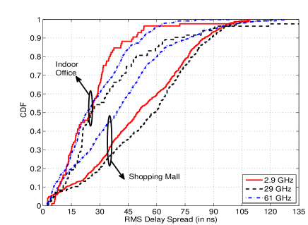
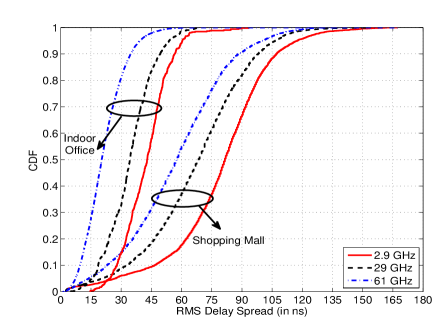
(a)	(b)
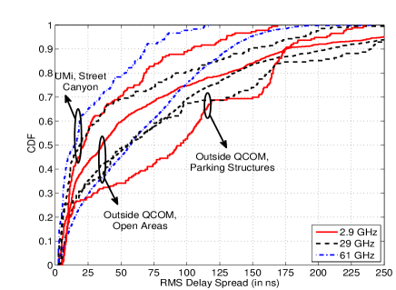
(c)	(d)

Figure 4: CDF of RMS delay spread in (a)-(b) indoor LOS and NLOS, and (c)-(d) outdoor LOS and NLOS settings.

III-B Delay Spread

The excess delay (denoted as $\tau_{\sf excess}$) and RMS delay spread (denoted as $\tau_{\sf rms}$) with omni-directional scans across different environments are studied. If $\tau_{i}$ and $p_{i}$ denote the delay and power corresponding to the $i$-th tap in a certain omni-directional scan, the excess delay and RMS delay spread are computed as:

$$\tau_{\sf excess} = \frac{\sum_{i}\tau_{i}p_{i}}{\sum_{i}p_{i}}$$ (7)

$$\tau_{\sf rms} = \sqrt{\frac{\sum_{i}\tau_{i}^{2}p_{i}}{\sum_{i}p_{i}}-\left(\frac{\sum_{i}\tau_{i}p_{i}}{\sum_{i}p_{i}}\right)^{2}}.$$ (8)

In the indoor office setting, the longest end-to-end delay is $250$ ns; any delay beyond this value is a result of reflections. For excess delay, an exponential distribution to the data for each link type and frequency band is fitted. The means of the exponential at $2.9$, $29$ and $61$ GHz for the excess delay of the combined third and fourth floor measurements with NLOS links are given by $\lambda^{-1}=93.4,82.3$ and $52.2$ ns, respectively. This trend is as expected given the difference in propagation characteristics at higher frequencies. The CDF of RMS delay spreads and the parameters associated with an exponential fit for NLOS links are provided in Fig. 4 and Table III, respectively. The corresponding numbers for the exponential fit to the excess delay at $2.9$, $29$ and $61$ GHz in the LOS case are $\lambda^{-1}=65.8$, $71.9$ and $33.3$ ns. For LOS links, the mean of the excess delay is actually higher at $29$ GHz. The RMS delay spread for LOS links illustrates this difference through a heavier tail at larger delay values.

The parameters associated with the RMS delay spread across all transmitter and receiver locations with omni-directional antenna scans at $2.9$, $29$ and $61$ GHz in the shopping mall are also presented in Table III for NLOS and LOS links. As in the indoor office setting, an increase in frequency reduces the RMS delay spread for NLOS links and the RMS delay spread for LOS links at $29$ GHz is in general larger than at $2.9$ GHz. Similar behavior is seen for the excess delay distributions. Table III also presents the RMS delay spread parameters for different scenarios in the outdoor case. In general, the delay spread in the outdoor setting is larger than in the indoor setting with some tail values corresponding to strong but significantly delayed sub-dominant clusters/paths.

The main conclusions from our studies are: i) Delay spread for NLOS links generally decrease with increase in frequency. ii) Delay spread for LOS links decrease with frequency in dense environments. iii) Delay spread for LOS links in non-dense environments shows an inconsistent behavior as frequency increases. While the literature does not offer a good explanation for this inconsistent behavior, the plausible explanations for it are:

• Waveguide effect where long enclosures such as walkways/corridors, dropped/false ceilings, etc., tend to propagate electromagnetic energy via alternate modes/more reflective paths decreasing the PLE (often even below the free-space PLE of $2$) and increasing the delay spread as frequency increases.

• Radar cross-section effect where seemingly small objects that do not participate in electromagnetic propagation at lower frequencies show up at higher frequencies. Such behavior happens as the wavelength approaches the roughness of surfaces (e.g., walls, light poles, etc.).

Since millimeter wave systems are likely to be used with beamforming, it is of interest in understanding the beamformed delay spread of the channel relative to that with an omni-directional scan. In this context, we note that in general, the beamformed delay spread is smaller than the omni delay spread. However, for most scenarios of interest in the indoor setting, this reduction is only by a small amount. A simple explanation for this observation is that indoor millimeter wave channels are sparse with few dominant clusters/paths. On the other hand, in the outdoor setting, the beamformed delay spread for the tail values can be significantly smaller than the omni delay spread. Thus, the effect of the significantly delayed sub-dominant clusters/paths get mitigated with beamforming.

TABLE III: Statistics of RMS Delay Spread

${\sf Metric}$	${\sf Parameter}$	${\sf f_{c}}=2.9\hskip 3.61371pt{\sf GHz}$		${\sf f_{c}}=29\hskip 3.61371pt{\sf GHz}$		${\sf f_{c}}=61\hskip 3.61371pt{\sf GHz}$
${\sf\bf Indoor\hskip 3.61371ptOffice}$		${\sf LOS}$	${\sf NLOS}$	${\sf LOS}$	${\sf NLOS}$	${\sf LOS}$	${\sf NLOS}$
${\sf Delay\hskip 3.61371ptspread}$	${\sf Median}$ $({\sf in\hskip 1.4457ptns})$	$25.72$	$42.89$	$25.39$	$34.34$	$23.10$	$20.36$
$\log_{10}({\sf Delay\hskip 3.61371ptspread})$	${\sf Mean}$	$-7.67$	$-7.39$	$-7.56$	$-7.49$	$-7.68$	$-7.72$
	${\sf Std.}$	$0.28$	$0.13$	$0.39$	$0.17$	$0.35$	$0.23$
${\sf\bf Shopping\hskip 3.61371ptMall}$		${\sf LOS}$	${\sf NLOS}$	${\sf LOS}$	${\sf NLOS}$	${\sf LOS}$	${\sf NLOS}$
${\sf Delay\hskip 3.61371ptspread}$	${\sf Median}$ $({\sf in\hskip 1.4457ptns})$	$50.0$	$81.5$	$59.0$	$68.5$	$39.0$	$57.5$
$\log_{10}({\sf Delay\hskip 3.61371ptspread})$	${\sf Mean}$	$-7.40$	$-7.15$	$-7.35$	$-7.23$	$-7.52$	$-7.31$
	${\sf Std.}$	$0.38$	$0.25$	$0.35$	$0.26$	$0.38$	$0.27$
${\sf\bf UMi,\hskip 3.61371ptStreet\hskip 3.61371ptCanyon}$		${\sf LOS}$	${\sf NLOS}$	${\sf LOS}$	${\sf NLOS}$	${\sf LOS}$	${\sf NLOS}$
${\sf Delay\hskip 3.61371ptspread}$	${\sf Median}$ $({\sf in\hskip 1.4457ptns})$	$21.75$	$99.0$	$18.75$	$87.25$	$14.75$	$74.5$
$\log_{10}({\sf Delay\hskip 3.61371ptspread})$	${\sf Mean}$	$-7.65$	$-7.02$	$-7.67$	$-7.11$	$-7.85$	$-7.18$
	${\sf Std.}$	$0.48$	$0.20$	$0.59$	$0.28$	$0.51$	$0.30$
${\sf\bf Outside\hskip 3.61371ptQCOM,\hskip 3.61371ptOpen\hskip 3.61371ptAreas}$		${\sf LOS}$	${\sf NLOS}$	${\sf LOS}$	${\sf NLOS}$	${\sf LOS}$	${\sf NLOS}$
${\sf Delay\hskip 3.61371ptspread}$	${\sf Median}$ $({\sf in\hskip 1.4457ptns})$	$35.5$	$105.0$	$55.5$	$67.0$	$57.0$	$11.0$
$\log_{10}({\sf Delay\hskip 3.61371ptspread})$	${\sf Mean}$	$-7.45$	$-7.15$	$-7.36$	$-7.36$	$-7.38$	$-7.95$
	${\sf Std.}$	$0.52$	$0.52$	$0.54$	$0.75$	$0.47$	$0.57$
${\sf\bf Outside\hskip 3.61371ptQCOM,\hskip 3.61371ptParking\hskip 3.61371ptStructures}$		${\sf LOS}$	${\sf NLOS}$	${\sf LOS}$	${\sf NLOS}$	${\sf LOS}$	${\sf NLOS}$
${\sf Delay\hskip 3.61371ptspread}$	${\sf Median}$ $({\sf in\hskip 1.4457ptns})$	$95.5$	$62.5$	$55.0$	$46.5$	$-$	$-$
$\log_{10}({\sf Delay\hskip 3.61371ptspread})$	${\sf Mean}$	$-7.26$	$-7.31$	$-7.38$	$-7.44$	$-$	$-$
	${\sf Std.}$	$0.52$	$0.43$	$0.62$	$0.51$	$-$	$-$

IV Material Measurements

Outdoor-to-indoor coverage critically depends on the reflection and penetration of mmW signals through various materials found in residential/office buildings such as sheetrock, concrete, glass, wood, etc.

IV-A Reflection Response

Towards this end, material measurements were performed with a completely synchronized signal generator and signal analyzer sweeping the $22$-$43$ GHz range. A horn antenna with rotational stages for easy adjustment of polarization, a gain of $25$ dBi and $10^{\sf o}$ beamwidth was used in the studies. The antenna was placed at about $1.5$-$2.5$ foot distance from the tested sample and incidence angles are varied in the studies. Absorber panels were used to contain reflections from the background objects surrounding the test site. A reference curve was obtained by placing a “perfect” reflecting plate (a $2\times 2$ sq ft aluminum plate) and sweeping over the same frequency range to obtain the reflected energy.

Reflection tests were conducted with different materials across a large range of incidence angles and for both parallel and perpendicular polarizations. For the sake of illustration, Figs. 5(a)-(b) illustrate the reflection response with a $5/8$ inch sheetrock material over the $22$-$43$ GHz range at parallel and perpendicular polarizations with an incidence angle of $18.5^{\sf o}$. The main observation here is that periodic notches that are several GHz wide and often with more than $30$ and $35$ dB in loss, respectively, are seen. These losses are attributed to changing material properties with frequency due to which signals constructively/destructively interfere from different surfaces that make the material. While a similar trend is observed across these experiments for both polarizations and different choices of incidence angles, the precise response at a frequency and the depth of the notches depend on the material, incidence angle and polarization.

Fig. 5(c) shows the more complicated (but realistic) response of a structured partition wall with multiple layers of materials (two sheetrock plates separated by a $4$ inch air gap) at $18.5^{\sf o}$ incidence angle and perpendicular polarization. The superposition of the response from the individual layers leads to complicated/periodic patterns across the frequency range (yellow curve), whereas the response of the single sheetrock alone is presented in the green curve. Fig. 5(d) illustrates the reflection response with a typical external wall material in the Qualcomm building, which is similar in behavior as Fig. 5(c).

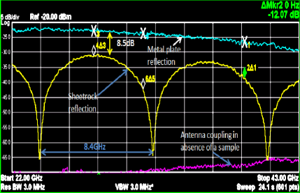
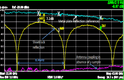
(a)	(b)
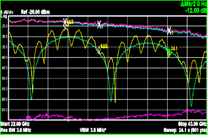
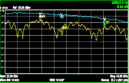
(c)	(d)

Figure 5: Material measurements illustrating reflection response over sheetrock using (a) parallel and (b) perpendicular polarizations. Response with (c) a structured partition wall, and (d) an external wall in the Qualcomm building across a range of mmW frequencies.

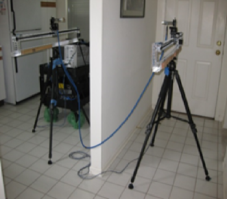
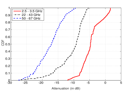
(a)	(b)

Figure 6: (a) Penetration loss measurement setup. (b) CDF of penetration loss with exterior walls in residential buildings.

IV-B Penetration Loss

We now consider studies with common residential wall materials to understand the scope of penetration loss for outdoor-to-indoor coverage and residential deployments. The measurement setup consists of two horn antennas (both with $10$ dBi gain) pointing at each other through the wall at a normal angle of incidence as in Fig. 6(a). The distance from the wall is about $0.5$ m for either antenna. For the measurements, the antennas are moved along and parallel to the wall with the receive antenna tracking the position of the transmit antenna in steps of $\sim 2.75$ mm over a $1$ m distance. The tests use a broadband sweep over $22$-$43$ GHz and $50$-$67$ GHz using a vector network analyzer and horn antennas. A broadband sweep is necessary to mitigate multi-surface reflections in the drywall and the complex wall structure. For reference, omni antenna measurements over the $2.5$-$3.5$ GHz range are also obtained.

From our studies, we first note that sheathing material made of strand boards (wood chips) involve the heavy use of glue, which has more attenuation at higher frequencies. This is reflected in Fig. 6(b) which illustrates the CDF of penetration loss with a strand board construction. In particular, median values of $4.7$, $9.2$ and $17.1$ dB are observed in the $2.5$-$3.5$, $22$-$43$ and $50$-$67$ GHz regimes, respectively. For walls made of plywood material, smaller losses that are comparable over a wide frequency range are observed. In particular, median values of $2.2$ and $3.0$ dB are seen in the $22$-$43$ and $50$-$67$ GHz regimes, respectively. Since strand board is typically lower cost than plywood, it is likely that newer/urban constructions as well as exterior residential walls are more likely to use strand board material than plywood material [34, p. 5]. Interior residential walls are more likely to be made of plywood material. Thus, it appears that outdoor-to-indoor coverage is more likely in older/residential settings than in urban settings.

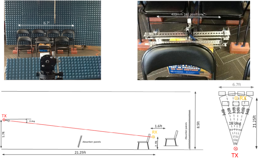
Figure 7: Layout of the stadium emulation experiments along with the linear measurement track, side view and top view of the setup.

IV-C Stadium Emulation

Another important aspect that needs understanding is the reflection/penetration of mmW signals from/through the human body. To understand this aspect, an experiment with two rows of improvised seats emulating a stadium setting is performed. The experimental setup is as shown in Fig. 7 with four people seated in the back row and three people in the front row. The back row is elevated over the front by four inches with the seats arranged in a staggered fashion. Chairs are made of metal covered with vinyl cushion. Absorbing panels are placed behind the back row and ground bounce is mitigated by absorbing panels on the floor.

A horn antenna with $20$ dBi gain and a beamwidth of $15^{\sf o}$ is placed at a distance of $6.5$ m, a height of $1.7$ m and at a downtilt angle of $98^{\sf o}$. An omni-directional antenna is placed behind the middle seat of the front row at $\approx{}4$ inches behind the first row and multiple measurements are made at $29$ GHz. The antenna is moved on a linear track every $\frac{1}{4}$ wavelength over $161$ positions (approx. $40$ cm) and measurements are obtained. Based on these measurements, it is observed that in general, human body scatters energy on to nearby geographic locations thereby aiding in stadium deployments by providing secondary bounces (alternate paths) for signaling when the LOS path in the boresight direction is blocked. To understand this observation, four controlled experiments are performed: i) no persons and no chairs (for baseline/reference), ii) one person with no surrounding chairs, iii) one person with all the surrounding chairs, and iv) seven persons in their respective chairs. Blockage loss is computed for the three latter scenarios relative to the baseline scenario of no persons and no chairs. Fig. 8 illustrates the CDF of blockage loss in these three scenarios. In particular, the effect of adjacent chairs reduces the blockage loss significantly from a median of $19.2$ dB to $14.9$ dB, and the presence of nearby humans improves the median further to $10.8$ dB. Thus, this study illustrates that these additional reflections and energy accumulation need to be modeled in stadium use-cases.

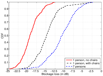
Figure 8: CDF of blockage loss in a stadium emulation.

V Implications on PHY Layer Design

Based on the measurements described in Sections. III-IV and comparisons of different figures-of-merit at identical transmit-receive location pairs across different frequencies, we make the following observations on the implications of these measurements on PHY layer/system design.

1. Indoor office, mall and outdoor deployments suggest the viability of good (but frequency-dependent) link margins with LOS links in a moderate number of cases. In scenarios with a far-field obstructed LOS path leading to a NLOS link, frequency-dependent shadow fading and path losses are observed. Losses at mmW frequencies (with respect to a reference distance of $d_{0}=1$ m) are typically higher than with sub-$6$ GHz systems in both indoor and outdoor settings. Nevertheless, the differential impact of mmW systems in terms of link margins relative to sub-$6$ GHz systems is not dramatically worse.

2. While we do not report these studies here, our initial work [35] as well as other similar works [36, 37, 38, 39, 40] in the literature (also, see the 3GPP Rel. 14 channel modeling document [7, pp. 49-52]) show that significant additional impairments due to human/hand blockages are observed at mmW frequencies.

3. Other works such as [29, 30] as well as our internal measurements point at significant losses due to foliage. In the outdoor-to-indoor coverage scenario, reflection response and penetration loss that are a function of material property, frequency, polarization and incident angle is observed. Further, deep notches that are several GHz wide are also seen. This motivates the need for system designs that support both frequency and spatial diversity.

4. The path, penetration and blockage losses at mmW frequencies along with typical equivalent isotropically radiated power (EIRP) constraints suggest that low pre-beamforming ${\sf SNR}$s are the norm in mmW systems. Thus, a viable system design has to overcome these huge losses. These losses can be bridged with beamforming array gains from the packing of a large number of antennas within the same array aperture [9, 10, 12, 11, 13, 14, 15]. Given the energy and complexity tradeoffs associated with large arrays, typical antenna geometries at the base-station are $64\times 4$, $32\times 8$, etc., with $2$-$16$ layer transmission.

5. In particular, subarray diversity is critical to overcome near-field obstructions such as those due to different parts of the human body that can significantly impair the received signal quality. This is also important to ensure coverage at the UE side over the entire angular space. Due to the smaller $\lambda$ at $60$ GHz (relative to $28$ GHz), more subarrays can be packed in the same area and such capabilities should be leveraged for better performance. While a large number of subarrays can be envisioned in a UE design, cost and complexity considerations suggest the use of $2$-$4$ layers with each layer independently controlling a subarray of $2$-$8$ antennas.

6. Clustering of multipath [41, 42] is an important macroscopic property that needs to be understood since the dominant clusters/angles capture the modes of propagation and are hence useful/relevant for multi-layer beamforming in transmission. This is a topic requiring careful attention and future work will address this aspect in detail. We point the readers to initial work in [43] which show that on average, $4$-$5$ clusters appear to be within a power differential of $5$ dB of each other motivating both directional transmissions and suggesting a high level of diversity. The viability of multiple modes suggests the use of both single-user MIMO strategies for increasing the peak rate as well as multi-user MIMO strategies for increasing the sum-rate [11, 44].

7. Practical beamforming algorithms should simultaneously optimize multiple criteria such as: i) good beamforming gain, ii) less unintended interference, iii) a link margin-dependent hierarchical solution for beamformer learning allowing a smooth tradeoff between beamforming gain and number of training samples, iv) robustness to channel dynamics, v) ability to work with different beamforming architectures, vi) a simpler network architecture that allows for a broadcast solution in initial UE discovery, etc. Coupled with higher antenna dimensionality in the mmW regime, the sparse and directional channel structure motivates the use of a certain subset of directional beamforming strategies [13, 14, 12, 45, 44, 46]. Such strategies allow a tradeoff between peak beamforming gain and initial UE discovery latency [14, 47, 48].

8. Given the small wavelengths, robust beam tracking is necessary to maintain the link gains even though the path parameters (gains and phases) change at much smaller time-scales. Further, given the significantly reduced interference due to a directional beam in unintended directions, the channel structure also motivates the use of simpler directional schedulers for user scheduling allowing dense spatial reuse and thus a higher network capacity [44, 46].

9. Frequency-dependent delay spreads are observed in NLOS settings with both omni-directional scans and directional beamforming. While delay spreads are small in most scenarios (for example, they are on the order of $30$-$50$ ns in indoor office, $50$-$90$ ns in shopping mall and $150$-$300$ ns in outdoor street canyon-type settings), there are also scenarios where a significantly large delay spread is seen (for example, even up to $800$ ns in certain outdoor open square settings with omni antennas). These extremes in outdoor settings can be attributed to radar cross-section effect. Supporting these extremes without incurring a high fixed system overhead (in terms of the cyclic prefix length for a multi-carrier design) is important.

10. In addition to the likelihood of multiple viable paths to a certain base-station, there are also viable paths to multiple base-stations [49, 50]. While the observation in [49] is based on ray-tracing, [50] is based on field measurements in both indoor and outdoor mobility studies. These observations suggest the criticality of a dense deployment of base-stations for robust mmW operation [3] and inter-base-station handover to leverage these paths. Integrated access and backhaul operation is highly desirable for small cell deployment [3].

11. Measurements emulating a stadium environment indicate that the presence of nearby humans can improve the received signal quality. These observations suggest the importance of not only modeling human blockage, but also reflection and energy accumulation from humans in such scenarios. These aspects require further investigation to address specular reflection and absorption.

VI Concluding Remarks

The main focus of this paper has been on a comparative study of propagation at $2.9$, $29$ and $61$ GHz across a large number of transmit-receive location pairs over different propagation environments (indoor office, shopping mall, outdoor settings, etc.). Our studies show that path loss at millimeter wave frequencies varies only less substantially relative to path loss at sub-$6$ GHz bands. On the other hand, delay spreads across LOS and NLOS links could vary substantially across frequencies. Furthermore, key differences are observed in terms of penetration of electromagnetic radiation across different materials commonly found in an indoor/residential setting. Deep notches in frequency response due to material properties suggest the use of frequency and spatial diversity schemes for communications. Human body scatters millimeter wave radiation to nearby geographic locations enhancing scenarios such as stadium coverage.

Observations from the studies described in this paper have already had a fundamental impact on channel models for $>{}6$ GHz systems. Studies on path loss, delay spread, material measurements, etc. have played a significant part in the multi-institutional channel modeling effort for $>{}6$ GHz systems [6]. The channel measurements are also used to obtain key system design guidelines on UE structure/geometry/design, beamforming, waveforms, etc. and these guidelines are important given the accelerated schedule of the Fifth Generation New Radio (5G NR) process at 3GPP and beyond. Results from the cited measurement campaigns highlight differences as strongly as consensus (as noted from [6]), illustrating the need for further extensive measurements in diverse settings. Of particular interest are more measurements on material propagation, blockage modeling, stadium use-case modeling, as well as simpler stochastic models that capture these measurements from a system level design perspective.

References

- [1] O. H. Koymen, A. Partyka, S. Subramanian, and J. Li, “Indoor mm-wave channel measurements: Comparative study of 2.9 GHz and 29 GHz,” Proc. IEEE Global Telecommun. Conf., San Diego, CA, pp. 1–6, Dec. 2015.
- [2] F. Khan and Z. Pi, “An introduction to millimeter wave mobile broadband systems,” IEEE Commun. Magaz., vol. 49, no. 6, pp. 101–107, June 2011.
- [3] N. Bhushan, J. Li, D. Malladi, R. Gilmore, D. Brenner, A. Damnjanovic, R. T. Sukhasvi, C. Patel, and S. Geirhofer, “Network densification: The dominant theme for wireless evolution into 5G,” IEEE Commun. Magaz., vol. 52, no. 2, pp. 82–89, Feb. 2014.
- [4] T. S. Rappaport, S. Sun, R. Mayzus, H. Zhao, Y. Azar, K. Wang, G. N. Wong, J. K. Schulz, M. K. Samimi, and F. Gutierrez, “Millimeter wave mobile communications for 5G cellular: It will work!” IEEE Access, vol. 1, pp. 335–349, 2013.
- [5] F. Boccardi, R. W. Heath, Jr., A. Lozano, T. L. Marzetta, and P. Popovski, “Five disruptive technology directions for 5G,” IEEE Commun. Magaz., vol. 52, no. 2, pp. 74–80, Feb. 2014.
- [6] Aalto University, AT&T, BUPT, CMCC, Ericsson, Huawei, Intel, KT Corporation, Nokia, NTT DOCOMO, NYU, Qualcomm, Samsung, U. Bristol, and USC, “White paper on ‘5G channel model for bands up to 100 GHz’,” v2.3, Oct. 2016.
- [7] RP-161301, 3GPP TR 38.900 V14.1.0 (2016-09), “Technical Specification Group Radio Access Network, Channel model for frequency spectrum above 6 GHz (Rel. 14),” Sept. 2016.
- [8] F. Rusek, D. Persson, B. K. Lau, E. G. Larsson, T. L. Marzetta, O. Edfors, and F. Tufvesson, “Scaling up MIMO: Opportunities and challenges with very large arrays,” IEEE Sig. Proc. Magaz., vol. 30, no. 1, pp. 40–60, Jan. 2013.
- [9] S. Hur, T. Kim, D. J. Love, J. V. Krogmeier, T. A. Thomas, and A. Ghosh, “Millimeter wave beamforming for wireless backhaul and access in small cell networks,” IEEE Trans. Commun., vol. 61, no. 10, pp. 4391–4403, Oct. 2014.
- [10] W. Roh, J.-Y. Seol, J. Park, B. Lee, J. Lee, Y. Kim, J. Cho, K. Cheun, and F. Aryanfar, “Millimeter-wave beamforming as an enabling technology for 5G cellular communications: Theoretical feasibility and prototype results,” IEEE Commun. Magaz., vol. 52, no. 2, pp. 106–113, Feb. 2014.
- [11] S. Sun, T. S. Rappaport, R. W. Heath, Jr., A. Nix, and S. Rangan, “MIMO for millimeter wave wireless communications: Beamforming, spatial multiplexing, or both?” IEEE Commun. Magaz., vol. 52, no. 12, pp. 110–121, Dec. 2014.
-
[12]
J. Brady, N. Behdad, and A. M. Sayeed, “Beamspace MIMO for millimeter-wave
communications: System architecture, modeling, analysis and measurements,”
IEEE Trans. Ant. Propagat., vol. 61, no. 7, pp. 3814–3827, July 2013,
Also, see CAP-MIMO architecture details and demonstration at
http://dune.ece.wisc.edu, Accessed on May 27, 2017. - [13] O. E. Ayach, S. Rajagopal, S. Abu-Surra, Z. Pi, and R. W. Heath, Jr., “Spatially sparse precoding in millimeter wave MIMO systems,” IEEE Trans. Wireless Commun., vol. 13, no. 3, pp. 1499–1513, Mar. 2014.
- [14] V. Raghavan, J. Cezanne, S. Subramanian, A. Sampath, and O. H. Koymen, “Beamforming tradeoffs for initial UE discovery in millimeter-wave MIMO systems,” IEEE Journ. Sel. Topics in Sig. Proc., vol. 10, no. 3, pp. 543–559, Apr. 2016.
- [15] S. Rangan, T. S. Rappaport, and E. Erkip, “Millimeter wave cellular networks: Potentials and challenges,” Proc. IEEE, vol. 102, no. 3, pp. 366–385, Mar. 2014.
- [16] A. Ghosh, T. A. Thomas, M. C. Cudak, R. Ratasuk, P. Moorut, F. W. Vook, T. S. Rappaport, G. R. MacCartney, Jr., S. Sun, and S. Nie, “Millimeter-wave enhanced local area systems: A high data-rate approach for future wireless networks,” IEEE Journ. Sel. Areas in Commun., vol. 32, no. 6, pp. 1152–1163, June 2014.
- [17] G. M. Rebeiz, RF MEMS: Theory, Design and Technology. Wiley Interscience, New York, NY, 2003.
- [18] L. Larson, “RF and microwave hardware challenges for future radio spectrum access,” Proc. IEEE, vol. 102, no. 3, pp. 321–333, Mar. 2014.
- [19] H. Krishnaswamy and H. Hashemi, “Integrated beamforming arrays,” In mm-Wave Silicon Technology, (A. M. Niknejad and H. Hashemi, Eds.), Springer, NY, pp. 243–295, 2008.
- [20] H. Xu, V. Kukshya, and T. S. Rappaport, “Spatial and temporal characteristics of 60 GHz indoor channels,” IEEE Journ. Sel. Areas in Commun., vol. 20, no. 3, pp. 620–630, Apr. 2002.
- [21] T. Zwick, T. J. Beukema, and H. Nam, “Wideband channel sounder with measurements and model for the 60 GHz indoor radio channel,” IEEE Trans. Veh. Tech., vol. 54, no. 4, pp. 1266–1277, July 2005.
- [22] P. F. M. Smulders, “Statistical characterization of 60 GHz indoor radio channels,” IEEE Ant. Propagat. Magaz., vol. 57, no. 10, pp. 2820–2829, Oct. 2009.
- [23] P. Okvist, H. Asplund, A. Simonsson, B. Halvarsson, J. Medbo, and N. Seifi, “15 GHz propagation properties assessed with 5G radio access prototype,” Proc. IEEE Intern. Symp. Personal Indoor Mobile Radio Commun., Hong Kong, pp. 2220–2224, Aug. 2015.
- [24] M. K. Samimi, K. Wang, Y. Azar, G. N. Wong, R. Mayzus, H. Zhao, J. K. Schulz, S. Sun, F. J. Gutierrez, and T. S. Rappaport, “28 GHz angle of arrival and angle of departure analysis for outdoor cellular communications using steerable beam antennas in New York City,” Proc. IEEE Veh. Tech. Conf. (Spring), Dresden, Germany, pp. 1–6, Sept. 2013.
- [25] Y. Azar, G. N. Wong, K. Wang, R. Mayzus, J. K. Schulz, H. Zhao, F. J. Gutierrez, D. Hwang, and T. S. Rappaport, “28 GHz propagation measurements for outdoor cellular communications using steerable beam antennas in New York City,” Proc. IEEE Intern. Conf. Commun., Budapest, Hungary, pp. 5143–5147, June 2013.
- [26] H. Zhao, R. Mayzus, S. Sun, M. K. Samimi, J. K. Schulz, Y. Azar, K. Wang, G. N. Wong, F. Gutierrez, and T. S. Rappaport, “28 GHz millimeter wave cellular communication measurements for reflection and penetration loss in and around buildings in New York City,” Proc. IEEE Intern. Conf. on Commun., Budapest, Hungary, pp. 5163–5167, June 2013.
- [27] T. S. Rappaport, E. Ben-Dor, J. Murdock, and Y. Qiao, “38 GHz and 60 GHz angle-dependent propagation for cellular and peer-to-peer wireless communications,” Proc. IEEE Intern. Conf. Commun., Ottawa, Canada, pp. 4568–4573, June 2012.
- [28] G. R. MacCartney, Jr. and T. S. Rappaport, “73 GHz millimeter wave propagation measurements for outdoor urban mobile and backhaul communications in New York City,” Proc. IEEE Intern. Conf. Commun., Sydney, Australia, pp. 4862–4867, June 2014.
- [29] F. Wang and K. Sarabandi, “An enhanced millimeter-wave foliage propagation model,” IEEE Trans. Ant. Propagat., vol. 53, no. 7, pp. 2138–2145, July 2005.
- [30] D. L. Jones, R. H. Espeland, and E. J. Violette, “Vegetation loss measurements at 9.6, 28.8, 57.6, and 96.1 GHz through a conifer orchard in Washington state,” U.S. Department of Commerce, NTIA Report 89-251, Tech. Rep., 1989.
- [31] ITU, “Recommendation P.833: Attenuation in vegetation,” Sept. 2016, Available: [Online]. https://www.itu.int/rec/R-REC-P.833/en.
- [32] S. Sun, T. S. Rappaport, S. Rangan, T. A. Thomas, A. Ghosh, I. Z. Kovács, I. Rodriguez, O. H. Koymen, A. Partyka, and J. Järveläinen, “Propagation path loss models for 5G urban micro and macro-cellular scenarios,” Proc. IEEE Veh. Tech. Conf. (Spring), Nanjing, China, pp. 1–5, May 2016.
- [33] S. Sun, T. S. Rappaport, T. A. Thomas, A. Ghosh, H. C. Nguyen, I. Z. Kovács, I. Rodriguez, O. H. Koymen, and A. Partyka, “Investigation of prediction accuracy, sensitivity, and parameter stability of large-scale propagation path loss models for 5G wireless communications,” IEEE Trans. Veh. Tech., vol. 65, no. 5, pp. 2843–2860, May 2016.
-
[34]
D. B. McKeever and J. Elling, “Wood products and other building materials
used in new residential construction in the United States with comparison to
previous studies,” June 2015,
Available: [Online]. http://www.apawood.org/Data/Sites/1/
documents/membersonly/marketreports/2015/residential
woodusagestudyus2012.pdf. - [35] Qualcomm, “Human and hand blockage modeling for GHz bands,” R1-161667, 3GPP TSG RAN WG1 #AH Channel Model, Ljubljana, Slovenia, Mar. 2016.
- [36] A. Maltsev et al., “Channel models for 60 GHz WLAN systems, doc: IEEE 802.11-09/0334r8,” 2010, Available: [Online]. https://mentor.ieee.org/802.11/documents.
- [37] M. Peter, M. Wisotzki, M. Raceala-Motoc, W. Keusgen, R. Felbecker, M. Jacob, S. Priebe, and T. Kuerner, “Analyzing human body shadowing at 60 GHz: Systematic wideband MIMO measurements and modeling approaches,” Proc. European Conf. Ant. and Propagat., pp. 468–472, Mar. 2012.
-
[38]
METIS 2020, “METIS channel model, Deliverable D1.4v3,” July 2015,
Available: [Online]. https://www.metis2020.com/wp-content/uploads/
deliverables/METIS_D1.4_v3.pdf. - [39] G. R. MacCartney, Jr., S. Deng, S. Sun, and T. S. Rappaport, “Millimeter-wave human blockage at 73 GHz with a simple double knife-edge diffraction model and extension for directional antennas,” Proc. IEEE Veh. Tech. Conf. (Fall), Montreal, Canada, pp. 1–6, Sept. 2016.
- [40] G. R. MacCartney, Jr. and T. S. Rappaport, “A flexible millimeter-wave channel sounder with absolute timing,” IEEE Journ. Sel. Areas in Commun., vol. 35, no. 6, pp. 1402–1418, June 2017.
- [41] B. H. Fleury, M. Tschudin, R. Heddergott, D. Dahlhaus, and K. I. Pedersen, “Channel parameter estimation in mobile radio environments using the SAGE algorithm,” IEEE Journ. Sel. Areas in Commun., vol. 17, no. 3, pp. 434–450, Mar. 1999.
- [42] N. Czink and P. Cera, “A novel framework for clustering parametric MIMO channel data including MPC powers,” COST 273 TD(05)104, Lisbon, Portugal, Nov. 2005.
- [43] Qualcomm, “Clustering methodology and results based on omni-directional and azimuthal scans in 29 and 61 GHz,” R1-161666, 3GPP TSG RAN WG1 #AH Channel Model, Ljubljana, Slovenia, Mar. 2016.
- [44] V. Raghavan, S. Subramanian, J. Cezanne, A. Sampath, O. H. Koymen, and J. Li, “Directional hybrid precoding in millimeter-wave MIMO systems,” Proc. IEEE Global Telecommun. Conf., Washington, DC, pp. 1–7, Dec. 2016.
- [45] V. Raghavan, S. Subramanian, J. Cezanne, and A. Sampath, “Directional beamforming for millimeter-wave MIMO systems,” Proc. IEEE Global Telecommun. Conf., San Diego, CA, pp. 1–7, Dec. 2015.
- [46] V. Raghavan, S. Subramanian, J. Cezanne, A. Sampath, O. H. Koymen, and J. Li, “Single-user vs. multi-user precoding for millimeter wave MIMO systems,” IEEE Journ. Sel. Areas in Commun., vol. 35, no. 6, pp. 1387–1401, June 2017.
- [47] C. N. Barati, S. A. Hosseini, S. Rangan, P. Liu, T. Korakis, S. S. Panwar, and T. S. Rappaport, “Directional cell discovery in millimeter wave cellular networks,” IEEE Trans. Wireless Commun., vol. 14, no. 12, pp. 6664–6678, Dec. 2015.
- [48] H. S.-Ghadikolaei, C. Fischione, G. Fodor, P. Popovski, and M. Zorzi, “Millimeter wave cellular networks: A MAC layer perspective,” IEEE Trans. Commun., vol. 63, no. 10, pp. 3437–3458, Oct. 2015.
- [49] Z. Zhang, J. H. Ryu, S. Subramanian, and A. Sampath, “Coverage and channel characteristics of millimeter wave band using ray tracing,” Proc. IEEE Intern. Conf. Commun., London, UK, pp. 1380–1385, June 2015.
- [50] V. Raghavan, A. Partyka, S. Subramanian, A. Sampath, O. H. Koymen, K. Ravid, J. Cezanne, K. K. Mukkavilli, and J. Li, “Millimeter wave MIMO prototype: Measurements and experimental results,” Submitted to IEEE Commun. Magaz., 2017.