Constrained Bayesian Optimization for Automatic Chemical Design

Abstract

Automatic Chemical Design is a framework for generating novel molecules with optimized properties. The original scheme, featuring Bayesian optimization over the latent space of a variational autoencoder, suffers from the pathology that it tends to produce invalid molecular structures. First, we demonstrate empirically that this pathology arises when the Bayesian optimization scheme queries latent points far away from the data on which the variational autoencoder has been trained. Secondly, by reformulating the search procedure as a constrained Bayesian optimization problem, we show that the effects of this pathology can be mitigated, yielding marked improvements in the validity of the generated molecules. We posit that constrained Bayesian optimization is a good approach for solving this class of training set mismatch in many generative tasks involving Bayesian optimization over the latent space of a variational autoencoder.

1 Introduction

There are two fundamental ways in which machine learning can be leveraged in chemical design:

1. To evaluate a molecule for a given application.

2. To find a promising molecule for a given application.

There has been much progress in the first use-case through the development of quantitative structure activity relationship (QSAR) models using deep learning [Ma et al., 2015]. These models have achieved state-of-the-art results in predicting properties Ryu et al. [2018a, b], Turcani et al. [2018], Dey et al. [2018], Coley et al. [2017], Gu et al. [2019], Zeng et al. [2018], Coley et al. [2019a] as well as property uncertainties Cortés-Ciriano and Bender [2018], Zhang and Lee [2019], Janet et al. [2019], Ryu et al. [2019] of known molecules.

The second use-case, finding new molecules that are useful for a given application, is arguably more important however. One existing approach for finding molecules that maximize an application-specific metric involves searching a large library of compounds, either physically or virtually Pyzer-Knapp et al. [2015], Playe [2019]. This has the disadvantage that the search is not open-ended; if the molecule is not in the library you specify, the search won’t find it.

A second method involves the use of genetic algorithms. In this approach, a known molecule acts as a seed and a local search is performed over a discrete space of molecules. Although these methods have enjoyed success in producing biologically active compounds, an approach featuring a search over an open-ended, continuous space would be beneficial. The use of geometrical cues such as gradients to guide the search in continuous space could accelerate both drug [Pyzer-Knapp et al., 2015, Gómez-Bombarelli et al., 2016] and materials [Hachmann et al., 2011, 2014] discovery by functioning as a high-throughput virtual screen of unpromising candidates.

Recently, Gómez-Bombarelli et al. [Gómez-Bombarelli et al., 2018] presented Automatic Chemical Design, a variational autoencoder (VAE) architecture capable of encoding continuous representations of molecules. In continuous latent space, gradient-based optimization is leveraged to find molecules that maximize a design metric.

Although a strong proof of concept, Automatic Chemical Design possesses a deficiency in so far as it fails to generate a high proportion of valid molecular structures. The authors hypothesize Gómez-Bombarelli et al. [2018] that molecules selected by Bayesian optimization lie in dead regions of the latent space far away from any data that the VAE has seen in training, yielding invalid structures when decoded.

The principle contribution of this paper is to present an approach based on constrained Bayesian optimization that generates a high proportion of valid sequences, thus solving the training set mismatch problem for VAE-based Bayesian optimization schemes.

2 Methods

2.1 SMILES Representation

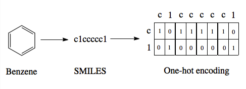
SMILES strings Weininger [1988] are a means of representing molecules as a character sequence. This text-based format facilitates the use of tools from natural language processing for applications such as chemical reaction prediction Schwaller et al. [2018a], Jin et al. [2017], Coley et al. [2019b], Schwaller et al. [2018b], Bradshaw et al. [2019a, b]. To make the SMILES representation compatible with the VAE architecture, the SMILES strings are in turn converted to one-hot vectors indicating the presence or absence of a particular character within a sequence as illustrated in Figure 1.

Figure 1: The SMILES representation and one-hot encoding for benzene. For purposes of illustration, only the characters present in benzene are shown in the one-hot encoding. In practice there is a column for each character in the SMILES alphabet.

2.2 Variational Autoencoders

Variational autoencoders Kingma and Welling [2014], Kingma et al. [2014] provide a means of mapping molecules $\mathbf{m}$ to and from continuous values $\mathbf{z}$ in a latent space. The encoding $\mathbf{z}$ is interpreted as a latent variable in a probabilistic generative model over which there is a prior distribution $p(\mathbf{z})$. The probabilistic decoder is defined by the likelihood function $p_{\theta}(\mathbf{m}|\mathbf{z})$. The posterior distribution $p_{\theta}(\mathbf{z}|\mathbf{m})$ is interpreted as the probabilistic encoder. The parameters of the likelihood $p_{\theta}(\mathbf{m}|\mathbf{z})$ as well as the parameters of the approximate posterior distribution $q_{\phi}(\mathbf{z}|\mathbf{m})$ are learned by maximizing the evidence lower bound (ELBO)

$$\mathcal{L}(\phi,\theta;\mathbf{m})=\mathbb{E}_{q_{\phi}(\mathbf{z}|\mathbf{m})}[\text{log}\>p_{\theta}(\mathbf{m},\mathbf{z})-\text{log}\>q_{\phi}(\mathbf{z}|\mathbf{m})].$$

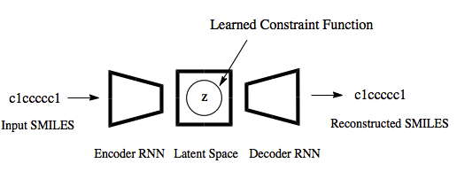
Variational autoencoders have been coupled with recurrent neural networks by Bowman et al. [2015] to encode sentences into a continuous latent space. This approach is followed for the SMILES format both by Gómez-Bombarelli et al. [2018] and here. The SMILES variational autoencoder, together with our constraint function, is shown in Figure 2.

Figure 2: The SMILES Variational Autoencoder with the learned constraint function illustrated by a circular feasible region in the latent space.

2.3 Objective Functions for Bayesian Optimization of Molecules

Bayesian optimization is performed in the latent space of the variational autoencoder in order to find molecules that score highly under a specified objective function. We assess molecular quality on the following objectives:

$$J^{\text{logP}}_{\text{comp}}(\textbf{z})=\text{logP}(\textbf{z})-\text{SA}(\textbf{z})-\text{ring-penalty}(\textbf{z}),$$

$$J^{\text{QED}}_{\text{comp}}(\textbf{z})=\text{QED}(\textbf{z})-\text{SA}(\textbf{z})-\text{ring-penalty}(\textbf{z}),$$

$$J^{\text{QED}}(\textbf{z})=\text{QED}(\textbf{z}).$$

z denotes a molecule’s latent representation, $\text{logP}(\textbf{z})$ is the water-octanol partition coefficient, $\text{QED}(\textbf{z})$ is the quantitative estimate of drug-likeness Bickerton et al. [2012] and $\text{SA}(\textbf{z})$ is the synthetic accessibility Ertl and Schuffenhauer [2009]. The ring penalty term is as featured in Gómez-Bombarelli et al. [2018]. The comp subscript is designed to indicate that the objective function is a composite of standalone metrics.

It is important to note, that the first objective, a common metric of comparison in this area, is mis-specified as had been pointed out by Griffiths et al. [2018]. From a chemical standpoint it is undesirable to maximize the logP score as is being done here. Rather it is preferable to optimize logP to be in a range that is in accordance with the Lipinski Rule of Five Lipinski et al. [1997]. We use the penalized logP objective here because regardless of its relevance for chemistry, it serves as a point of comparison against other methods.

2.4 Constrained Bayesian Optimization of Molecules

We now describe our extension to the Bayesian optimization procedure followed by Gómez-Bombarelli et al. [2018]. Expressed formally, the constrained optimization problem is

$$\max_{\textbf{z}}f(\textbf{z})\>\text{s.t.}\>\text{Pr}(\mathcal{C}(\textbf{z}))\geq 1-\delta$$

where $f(\textbf{z})$ is a black-box objective function, $\Pr(\mathcal{C}(\textbf{z}))$ denotes the probability that a Boolean constraint $\mathcal{C}(\textbf{z})$ is satisfied and $1-\delta$ is some user-specified minimum confidence that the constraint is satisfied Gelbart et al. [2014]. The constraint is that a latent point must decode successfully a large fraction of the times decoding is attempted. The specific fractions used are provided in the results section. The black-box objective function is noisy because a single latent point may decode to multiple molecules when the model makes a mistake, obtaining different values under the objective. In practice, ${f(\textbf{z})}$ is one of the objectives listed in section 2.3.

2.5 Expected Improvement with Constraints (EIC)

EIC may be thought of as expected improvement (EI),

$$\text{EI}(\textbf{z})=\mathbb{E}_{f(\textbf{z})}\big{[}\max(0,f(\textbf{z})-\eta)\big{]},$$

that offers improvement only when a set of constraints are satisfied [Schonlau et al., 1998]:

$$\text{EIC}(\textbf{z})=\text{EI}(\textbf{z})\Pr(\mathcal{C}(\textbf{z})).$$

The incumbent solution $\eta$ in $\text{EI}(\textbf{z})$, may be set in an analogous way to vanilla expected improvement Gelbart [2015] as either:

1. The best observation in which all constraints are observed to be satisfied.

2. The minimum of the posterior mean such that all constraints are satisfied.

The latter approach is adopted for the experiments performed in this paper. If at the stage in the Bayesian optimization procedure where a feasible point has yet to be located, the form of acquisition function used is that defined by [Gelbart, 2015]

$$\text{EIC}(\textbf{z})=\left\{\begin{array}[]{cc}\Pr(\mathcal{C}(\textbf{z})\text{EI}(\textbf{z}),&\text{if}\>\>\exists\textbf{z},\>\Pr(\mathcal{C}(\textbf{z}))\geq 1-\delta\\ \>\>\>\>\>\Pr(\mathcal{C}(\textbf{z})),\phantom{\text{EI}(m)}&\text{otherwise}\\ \end{array}\right.$$

with the intuition being that if the probabilistic constraint is violated everywhere, the acquisition function selects the point having the highest probability of lying within the feasible region. The algorithm ignores the objective until it has located the feasible region.

3 Related Work

The literature concerning generative models of molecules has exploded since the first work on the topic Gómez-Bombarelli et al. [2018]. Current methods feature molecular representations such as SMILES [Janz et al., 2018, Segler et al., 2017, Blaschke et al., 2017, Skalic et al., 2019, Ertl et al., 2017, Lim et al., 2018, Kang and Cho, 2018, Sattarov et al., 2019, Gupta et al., 2018, Harel and Radinsky, 2018, Yoshikawa et al., 2018, Bjerrum and Sattarov, 2018, Mohammadi et al., 2019] and graphs [Simonovsky and Komodakis, 2018, Li et al., 2018a, Jin et al., 2018, De Cao and Kipf, 2018, Kusner et al., 2017, Dai et al., 2018, Samanta et al., 2019, Li et al., 2018b, Kajino, 2019, Jin et al., 2019, Bresson and Laurent, 2019, Lim et al., 2019, Pölsterl and Wachinger, 2019, Krenn et al., 2019, Maziarka et al., 2019, Madhawa et al., 2019, Shen, 2018, Korovina et al., 2019] and employ reinforcement learning Guimaraes et al. [2017], Zhou et al. [2019], Putin et al. [2018a], You et al. [2018], Putin et al. [2018b], Yang et al. [2017], Wei et al. [2019], Ståhl et al. [2019], Kraev [2018], Olivecrona et al. [2017], Popova et al. [2019] as well as generative adversarial networks Prykhodko et al. [2019] for the generative process. These methods are well-summarized by a number of recent review articles [Xue et al., 2019, Elton et al., 2019, Schwalbe-Koda and Gómez-Bombarelli, 2019, Chang, 2019, Sanchez-Lengeling and Aspuru-Guzik, 2018a]. In this work we focus solely on VAE-based Bayesian optimization schemes for molecule generation and so we do not benchmark model performance against the aforementioned methods. Principally, we are concerned with highlighting the issue of training set mismatch in VAE-based Bayesian optimizations schemes and demonstrating the superior performance of a constrained Bayesian optimization approach.

4 Results and discussion

4.1 Experiment I: Drug Design

In this section we conduct an empirical test of the hypothesis from [Gómez-Bombarelli et al., 2018] that the decoder’s lack of efficiency is due to data point collection in dead regions of the latent space far from the data on which the VAE was trained. We use this information to construct a binary classification Bayesian Neural Network (BNN) to serve as a constraint function that outputs the probability of a latent point being valid, the details of which will be discussed in the section on labelling criteria. Secondly, we compare the performance of our constrained Bayesian optimization implementation against the original model (baseline) in terms of the numbers of valid and drug-like molecules generated. Thirdly, we compare the quality of the molecules produced by constrained Bayesian optimization with those of the baseline model. The code for all experiments has been made publicly available at https://github.com/Ryan-Rhys/Constrained-Bayesian-Optimisation-for-Automatic-Chemical-Design

4.1.1 Implementation

The implementation details of the encoder-decoder network as well as the sparse GP for modelling the objective remain unchanged from [Gómez-Bombarelli et al., 2018]. For the constrained Bayesian optimization algorithm, the BNN is constructed with $2$ hidden layers each $100$ units wide with ReLU activation functions and a logistic output. Minibatch size is set to $1000$ and the network is trained for $5$ epochs with a learning rate of 0.0005. $20$ iterations of parallel Bayesian optimization are performed using the Kriging-Believer algorithm in all cases. Data is collected in batch sizes of $50$. The same training set as [Gómez-Bombarelli et al., 2018] is used, namely $249,456$ drug-like molecules drawn at random from the ZINC database [Irwin et al., 2012].

4.1.2 Diagnostic Experiments and Labelling Criteria

These experiments were designed to test the hypothesis that points collected by Bayesian optimization lie far away from the training data in latent space. In doing so, they also serve as labelling criteria for the data collected to train the BNN acting as the constraint function. The resulting observations are summarized in Figure 3.

(a) % Valid Molecules

(b) % Methane Molecules

(c) % Drug-like Molecules

Figure 3: Experiments on $5$ disjoint sets comprising $50$ latent points each. Very small (VS) Noise are training data latent points with approximately $1\%$ noise added to their values, Small (S) Noise have $10\%$ noise added to their values and Big (B) Noise have $50\%$ noise added to their values. All latent points underwent $500$ decode attempts and the results are averaged over the $50$ points in each set. The percentage of decodings to: a) valid molecules b) methane molecules. c) drug-like molecules.

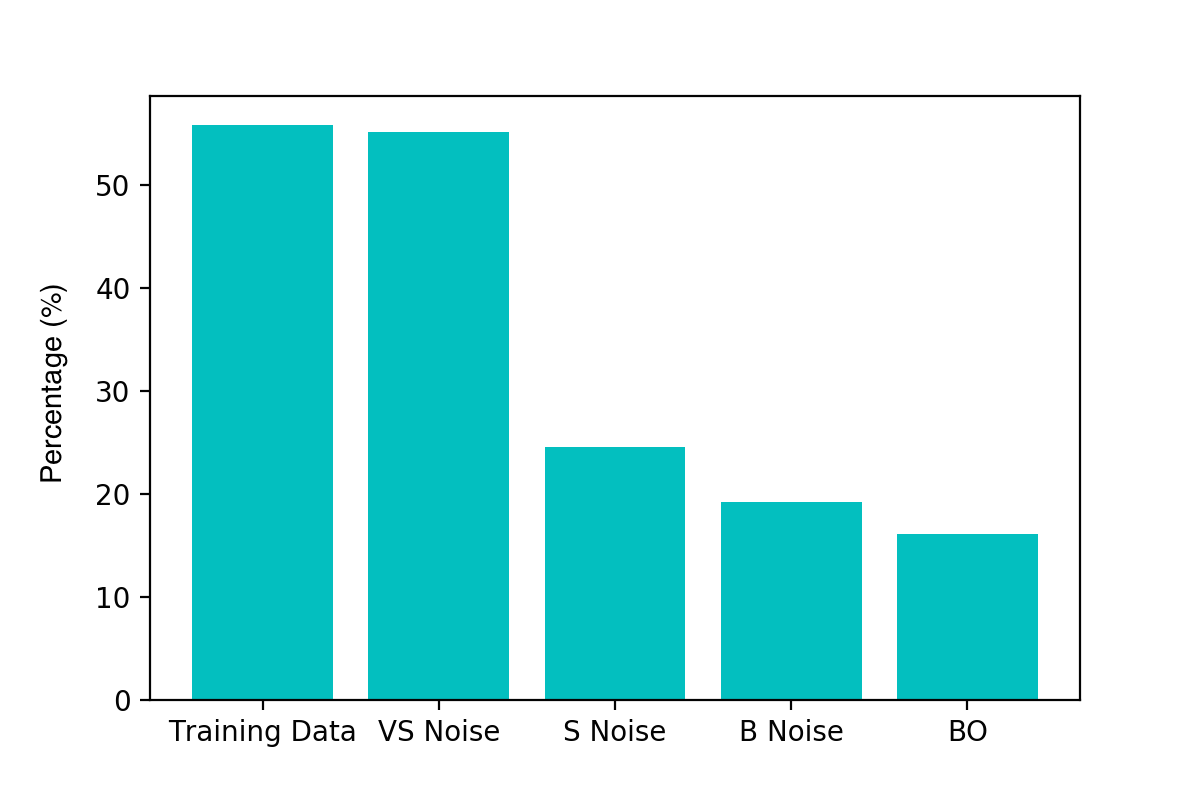
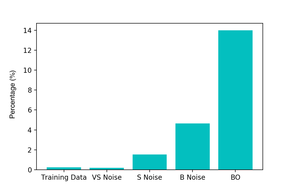
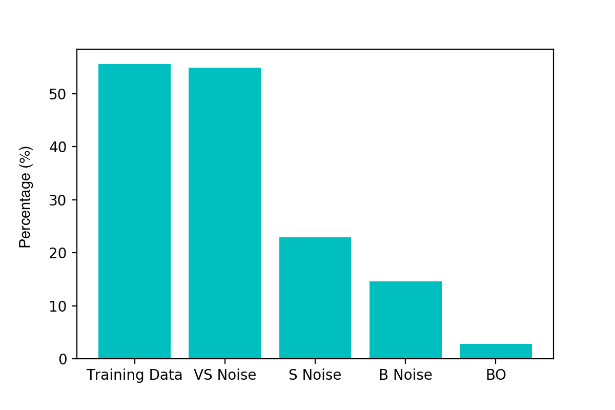
There is a noticeable decrease in the percentage of valid molecules decoded as one moves further away from the training data in latent space. Points collected by Bayesian optimization do the worst in terms of the percentage of valid decodings. This would suggest that these points lie farthest from the training data. The decoder over-generates methane molecules when far away from the data. One hypothesis for why this is the case is that methane is represented as ’C’ in the SMILES syntax and is by far the most common character. Hence far away from the training data, combinations such as ’C’ followed by a stop character may have high probability under the distribution over sequences learned by the decoder.

Given that methane has far too low a molecular weight to be a suitable drug candidate, a third plot, 3(c), shows the percentage of decoded molecules such that the molecules are both valid and have a tangible molecular weight. The definition of a tangible molecular weight was interpreted somewhat arbitrarily as a SMILES length of $5$ or greater. Henceforth, molecules that are both valid and have a SMILES length greater than $5$ will be loosely referred to as drug-like. This is not to imply that a molecule comprising five SMILES characters is likely to be drug-like, but rather this SMILES length serves the purpose of determining whether the decoder has been successful or not.

As a result of these diagnostic experiments, it was decided that the criteria for labelling latent points to initialize the binary classification neural network for the constraint would be the following: if the latent point decodes into drug-like molecules in more than $20\%$ of decode attempts, it should be classified as drug-like and non drug-like otherwise.

4.1.3 Molecular Validity

The BNN for the constraint was initialized with $117,440$ positive class points and $117,440$ negative class points. The positive points were obtained by running the training data through the decoder assigning them positive labels if they satisfied the criteria outlined in the previous section. The negative class points were collected by decoding points sampled uniformly at random across the $56$ latent dimensions of the design space. Each latent point undergoes $100$ decode attempts and the most probable SMILES string is retained. $J^{\text{logP}}_{\text{comp}}(\textbf{z})$ is the choice of objective function. The relative performance of constrained Bayesian optimization and unconstrained Bayesian optimization (baseline) [Gómez-Bombarelli et al., 2018] is compared in Figure 4.

(a) Drug-like Molecules

(b) New Drug-like Molecules

Figure 4: a) The percentage of latent points decoded to drug-like molecules. The results are from 20 iterations of Bayesian optimization with batches of 50 data points collected at each iteration (1000 latent points decoded in total). The standard error is given for 5 separate train/test set splits of 90/10.

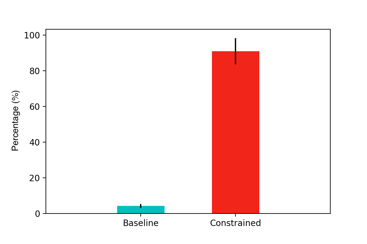
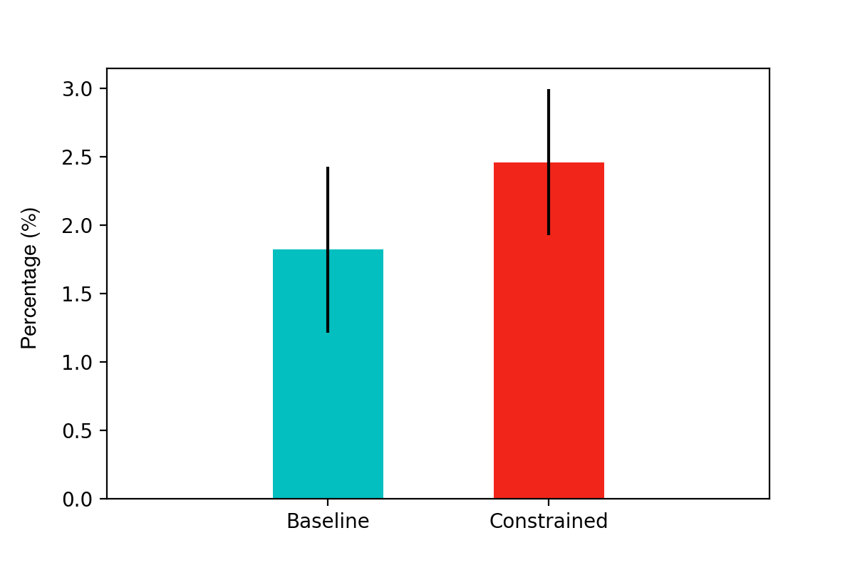
The results show that greater than $80\%$ of the latent points decoded by constrained Bayesian optimization produce drug-like molecules compared to less than $5\%$ for unconstrained Bayesian optimization. One must account however, for the fact that the constrained approach may be decoding multiple instances of the same novel molecules. Constrained and unconstrained Bayesian optimization are compared on the metric of the percentage of unique novel molecules produced in 4(b).

One may observe that constrained Bayesian optimization outperforms unconstrained Bayesian optimization in terms of the generation of unique molecules, but not by a large margin. A manual inspection of the SMILES strings collected by the unconstrained optimization approach showed that there were many strings with lengths marginally larger than the cutoff point, which is suggestive of partially decoded molecules. As such, a fairer metric for comparison should be the quality of the new molecules produced as judged by the scores from the black-box objective function. This is examined next.

4.1.4 Molecular Quality

(a) Composite LogP

(b) Composite QED

(c) QED

Figure 5: The best scores for new molecules generated from the baseline model (blue) and the model with constrained Bayesian optimization (red). The vertical lines show the best scores averaged over 5 separate train/test splits of 90/10. For reference, the histograms are presented against the backdrop of the top 10% of the training data in the case of Composite LogP and QED, and the top 20% of the training data in the case of Composite QED.

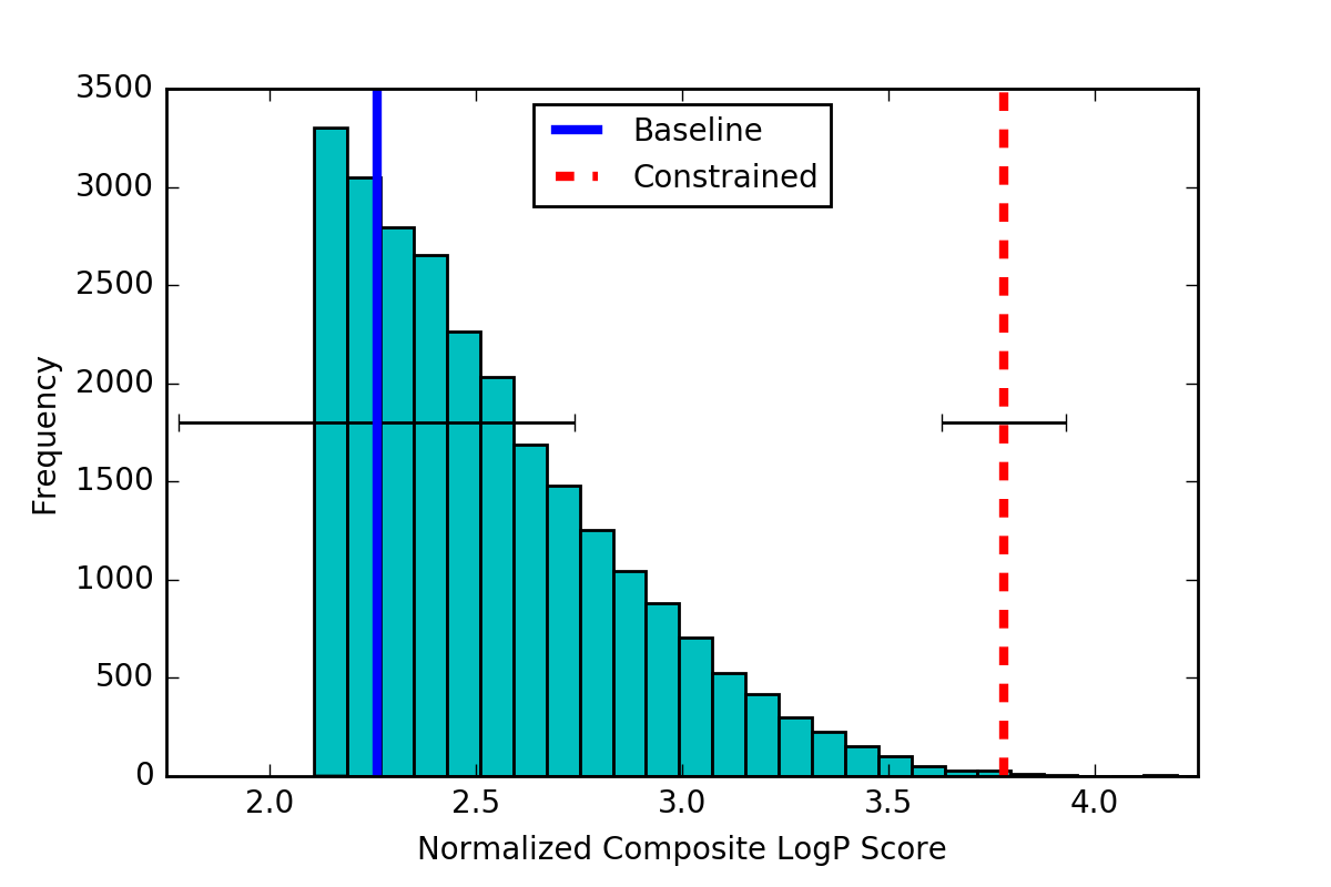
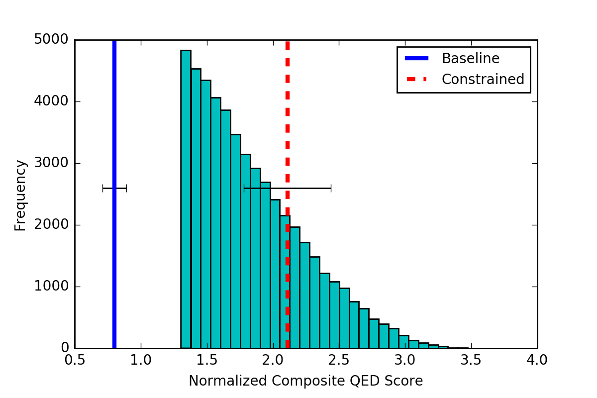
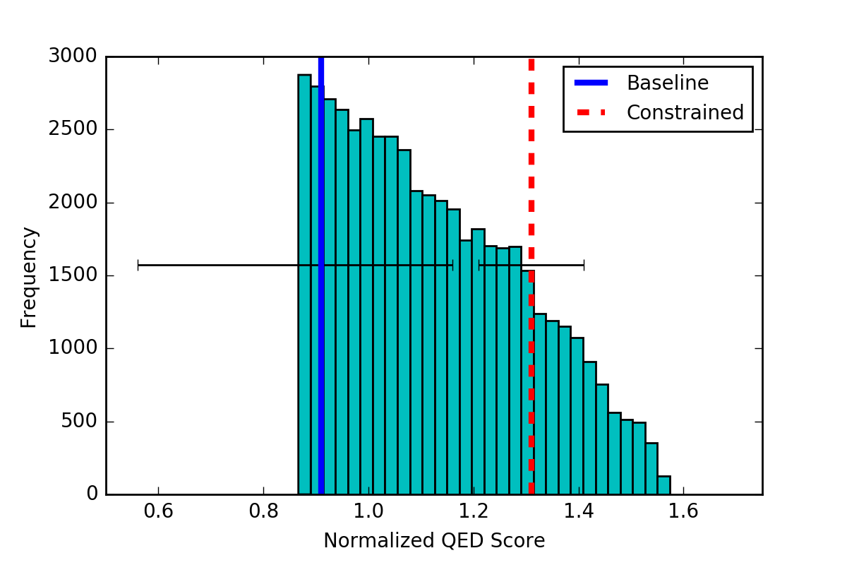
The results of Figure 5 indicate that constrained Bayesian optimization is able to generate higher quality molecules relative to unconstrained Bayesian optimization across the three drug-likeness metrics introduced in section 2.3. Over the $5$ independent runs, the constrained optimization procedure in every run produced new drug-like molecules ranked in the 100th percentile of the distribution over training set scores for the $J^{\text{logP}}_{\text{comp}}(\textbf{z})$ objective and over the 90th percentile for the remaining objectives. Table 1 gives the percentile that the averaged score of the new molecules found by each process occupies in the distribution over training set scores.

Table 1: Percentile of the averaged new molecule score relative to the training data. The results of 5 separate train/test set splits of 90/10 are provided.

Objective	Baseline	Constrained
LogP Composite	36$\pm$ 14	92$\pm$ 4
QED Composite	14$\pm$ 3	72$\pm$ 10
QED	11$\pm$ 2	79$\pm$ 4

4.2 Experiment II: Material Design

In order to show that the constrained Bayesian optimization approach is extensible beyond the realm of drug design, we trained the model on data from the Harvard Clean Energy Project [Hachmann et al., 2011, 2014] to generate molecules optimized for power conversion efficiency (PCE).

4.2.1 Implementation

A neural network was trained to predict the PCE of $200,000$ molecules drawn at random from the Harvard Clean Energy Project dataset using 512-bit Morgan circular fingerprints Rogers and Hahn [2010] as input features with bond radius of $2$ using RDKit Landrum [2016]. If unmentioned the details of the implementation remain the same as experiment I.

4.2.2 PCE Scores

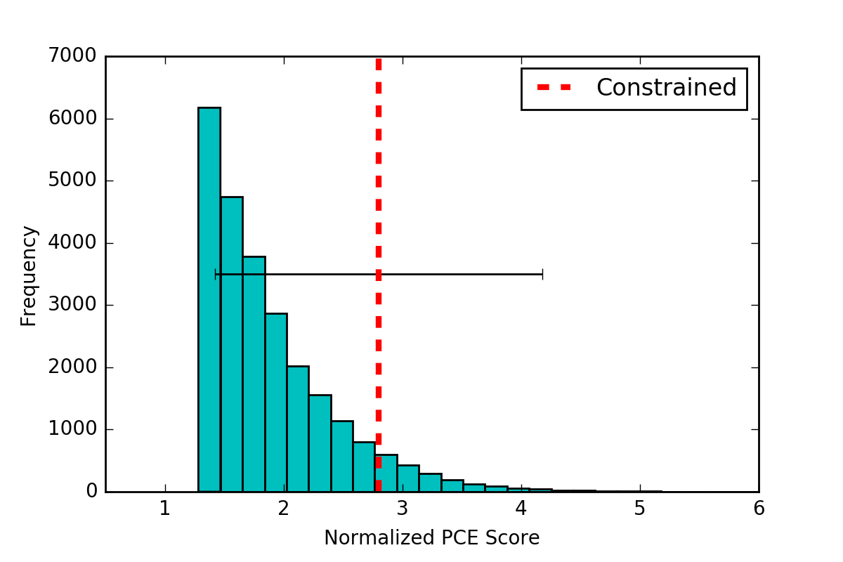
The results are given in Figure 6. The averaged score of the new molecules generated lies above the 90th percentile in the distribution over training set scores. Given that the objective function in this instance was learned using a neural network, advances in predicting chemical properties from data Duvenaud et al. [2015], Ramsundar et al. [2015] are liable to yield concomitant improvements in the optimized molecules generated through this approach.

Figure 6: The best scores for novel molecules generated by the constrained Bayesian optimization model optimizing for PCE. The results are averaged over 3 separate runs with train/test splits of 90/10.

5 Concluding Remarks

The reformulation of the search procedure in the Automatic Chemical Design model as a constrained Bayesian optimization problem has led to concrete improvements on two fronts:

1. Validity - The number of valid molecules produced by the constrained optimization procedure offers a marked improvement over the original model.

2. Quality - For five independent train/test splits, the scores of the best molecules generated by the constrained optimization procedure consistently ranked above the 90th percentile of the distribution over training set scores for all objectives considered.

These improvements provide strong evidence that constrained Bayesian optimization is a good solution method for the training set mismatch pathology present in the unconstrained approach for molecule generation. More generally, we foresee that constrained Bayesian optimization is a workable solution to the training set mismatch problem in any VAE-based Bayesian optimization scheme. Our code is made publicly available at https://github.com/Ryan-Rhys/Constrained-Bayesian-Optimisation-for-Automatic-Chemical-Design. Further work could feature improvements to the constraint scheme Rainforth et al. [2016], Mahmood and Hernández-Lobato [2019], Astudillo and Frazier [2019], 2018_Phoenics [201], Moriconi et al. [2019], Bartz-Beielstein and Zaefferer [2017]. In terms of objectives for molecule generation, recent work by Blaschke et al. [2017], Polykovskiy et al. [2018a], Tabor et al. [2018], Aumentado-Armstrong [2018], Sanchez-Lengeling and Aspuru-Guzik [2018b] has featured a more targeted search for novel compounds. This represents a move towards more industrially-relevant objective functions for Bayesian Optimization which should ultimately replace the chemically mis-specified objectives, such as the penalized logP score, identified both here and in Griffiths et al. [2018]. In addition, efforts at benchmarking generative models of molecules Brown et al. [2019], Polykovskiy et al. [2018b] should also serve to advance the field.

Appendix A Toy Experiment: The Branin-Hoo Function

The Branin-Hoo function is a toy problem on which to test the functionality of the algorithmic implementation for constrained Bayesian optimization. The particular variant of the Branin-Hoo optimization of interest here is the constrained formulation of the problem as featured in [Gelbart et al., 2014]. This Branin-Hoo function has three global minima at the coordinates $(-\pi,12.275),(\pi,2.275)\>\>\text{and}\>\>(9.42478,2.475)$. In order to formulate the problem as a constrained optimization problem, a disk constraint on the region of feasible solutions is introduced. In contrast to the formulation of the problem in [Gelbart et al., 2014], the disk constraint is coupled in this scenario in the sense that the objective and the constraint will be evaluated jointly at each iteration of Bayesian optimization. In addition, the observations of the black-box objective function will be assumed to be noise-free. The minima of the Branin-Hoo function as well as the disk constraint are illustrated in  Figure 7.

(a) Minima Locations

(b) Disk Constraint

Figure 7: Constrained Bayesian optimization of the 2D Branin-Hoo Function.

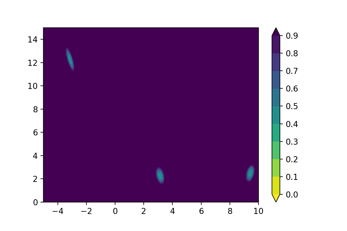
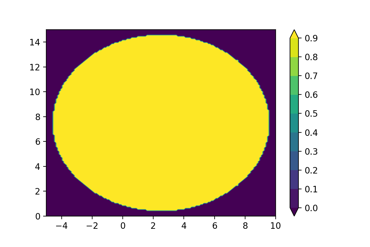
The disk constraint eliminates the upper-left and lower-right solutions, leaving a unique global minimum at $(\pi,2.275)$. Given that our implementation of constrained Bayesian optimization relies on the use of a sparse GP as the underlying statistical model of the black-box objective and as such is designed for scale as opposed to performance, the results will not be compared directly against those of [Gelbart et al., 2014] who use an exact GP to model the objective. It will be sufficient to compare the performance of the algorithm against random sampling. Both the sequential Bayesian optimization algorithm and the parallel implementation using the Kriging-Believer algorithm are tested.

A.1 Implementation

A Sparse GP featuring the FITC approximation, based on the implementation of [Bui et al., 2016] is used to model the black-box objective function. The kernel choice is exponentiated quadratic with automatic relevance determination (ARD). The number of inducing points $M$ was chosen to be $20$ in the case of sequential Bayesian optimization, and $5$ in the case of parallel Bayesian optimization using the Kriging-Believer algorithm. The sparse GP is trained for 400 epochs using Adam [Kingma and Ba, 2014] with the default parameters and a learning rate of $0.005$. The minibatch size is chosen to be $5$. The extent of jitter is chosen to be $0.00001$. A Bayesian Neural Network (BNN), adapted from the MNIST digit classification network of [Hernández-Lobato et al., 2016] is trained using black-box alpha divergence minimization to model the constraint.

The network has a single hidden layer with $50$ hidden units, Gaussian activation functions and logistic output units. The mean parameters of $q$, the approximation to the true posterior, are initialized by sampling from a zero-mean Gaussian with variance $\frac{2}{d_{\text{in}}+d_{\text{out}}}$ according to the method of [Glorot and Bengio, 2010], where $d_{\text{in}}$ is the dimension of the previous layer in the network and $d_{\text{out}}$ is the dimension of the next layer in the network. The value of $\alpha$ is taken to be $0.5$, minibatch sizes are taken to be $10$ and $50$ Monte Carlo samples are used to approximate the expectations with respect to $q$ in each minibatch. The BNN adapted from [Hernández-Lobato et al., 2016] was implemented in the Theano library [Theano Development Team, 2016]. The LBFGs method [Liu and Nocedal, 1989] was used to optimize the EIC acquisition function in all experiments.

A.2 Results

The results of the sequential constrained Bayesian optimization algorithm with EIC are shown in  Figure 8. The algorithm was initialized with $50$ labeled data points drawn uniformly at random from the grid depicted. $40$ iterations of Bayesian optimization were carried out.

(a) Collected Data Points

(b) Objective Predictive Mean

(c) $\Pr(\mathcal{C}(\mathbf{x})\geq 0)$

Figure 8: a) Data points collected over 40 iterations of sequential Bayesian optimization. b) Contour plot of the predictive mean of the sparse GP used to model the objective function. Lighter colours indicate lower values of the objective. c) The contour learned by the BNN giving the probability of constraint satisfaction.

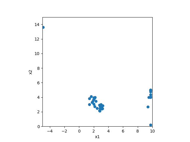
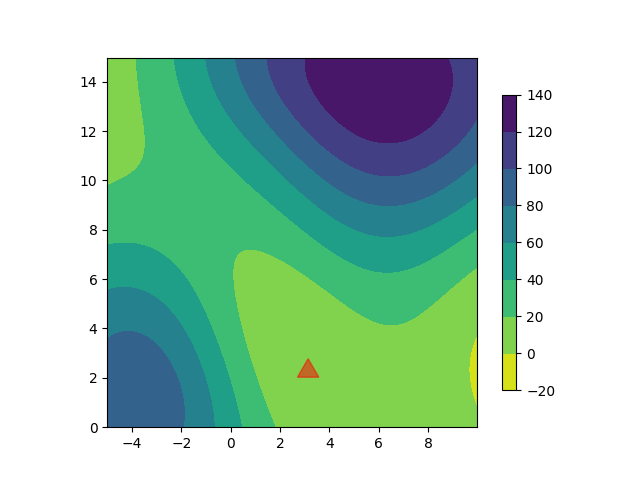
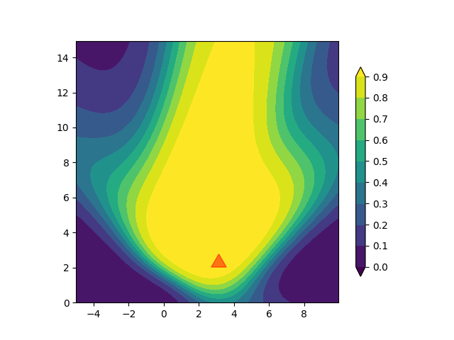
The figures show that the algorithm is correctly managing to collect data in the vicinity of the single feasible minimum. Figure 9 compares the performance of parallel Bayesian optimization using the Kriging-Believer algorithm against the results of random sampling. Both algorithms were initialized using $10$ data points drawn uniformly at random from the grid on which the Branin-Hoo function is defined and were run for $10$ iterations of Bayesian optimization. At each iteration a batch of $5$ data points was collected for evaluation.

Figure 9: Performance of Parallel Bayesian Optimization with EIC against Random Sampling.

After $10$ iterations, the minimum feasible value of the objective function was $0.42$ for parallel Bayesian optimization with EIC using the Kriging-Believer algorithm and $2.63$ for random sampling. The true minimum feasible value is $0.40$.

A.3 Discussion

The Branin-Hoo experiment is designed to yield some visual intuition for the constrained Bayesian Optimization implementation in two dimensions before moving to higher dimensional molecular space. The results demonstrate that the implementation of constrained Bayesian optimization is behaving as expected in so far as the constraint in the problem is recognized and the search procedure outperforms random sampling.

It could be worth performing some investigation into how much worse the sparse GP performs relative to the full GP in the constrained setting. Another aspect that could be explored is the impact of the initialization. It has recently been argued that different algorithms will vary in their performance depending on how much information about the design space there is available [Morar et al., 2017].

References

- Ma et al. [2015] Junshui Ma, Robert P Sheridan, Andy Liaw, George E Dahl, and Vladimir Svetnik. Deep neural nets as a method for quantitative structure–activity relationships. Journal of Chemical Information and Modeling, 55(2):263–274, 2015.
- Ryu et al. [2018a] Seongok Ryu, Jaechang Lim, Seung Hwan Hong, and Woo Youn Kim. Deeply learning molecular structure-property relationships using attention-and gate-augmented graph convolutional network. arXiv preprint arXiv:1805.10988, 2018a.
- Ryu et al. [2018b] Jae Yong Ryu, Hyun Uk Kim, and Sang Yup Lee. Deep learning improves prediction of drug–drug and drug–food interactions. Proceedings of the National Academy of Sciences, 115(18):E4304–E4311, 2018b.
- Turcani et al. [2018] Lukas Turcani, Rebecca L Greenaway, and Kim E Jelfs. Machine learning for organic cage property prediction. Chemistry of Materials, 31(3):714–727, 2018.
- Dey et al. [2018] Sanjoy Dey, Heng Luo, Achille Fokoue, Jianying Hu, and Ping Zhang. Predicting adverse drug reactions through interpretable deep learning framework. BMC Bioinformatics, 19(21):476, 2018.
- Coley et al. [2017] Connor W Coley, Regina Barzilay, William H Green, Tommi S Jaakkola, and Klavs F Jensen. Convolutional embedding of attributed molecular graphs for physical property prediction. Journal of Chemical Information and Modeling, 57(8):1757–1772, 2017.
- Gu et al. [2019] Geun Ho Gu, Juhwan Noh, Inkyung Kim, and Yousung Jung. Machine learning for renewable energy materials. Journal of Materials Chemistry A, 7:17096–17117, 2019. doi: 10.1039/C9TA02356A. URL http://dx.doi.org/10.1039/C9TA02356A.
- Zeng et al. [2018] Minggang Zeng, Jatin Nitin Kumar, Zeng Zeng, Ramasamy Savitha, Vijay Ramaseshan Chandrasekhar, and Kedar Hippalgaonkar. Graph convolutional neural networks for polymers property prediction. arXiv preprint arXiv:1811.06231, 2018.
- Coley et al. [2019a] Connor W Coley, Wengong Jin, Luke Rogers, Timothy F Jamison, Tommi S Jaakkola, William H Green, Regina Barzilay, and Klavs F Jensen. A graph-convolutional neural network model for the prediction of chemical reactivity. Chemical Science, 10(2):370–377, 2019a.
- Cortés-Ciriano and Bender [2018] Isidro Cortés-Ciriano and Andreas Bender. Deep confidence: a computationally efficient framework for calculating reliable prediction errors for deep neural networks. Journal of Chemical Information and Modeling, 59(3):1269–1281, 2018.
- Zhang and Lee [2019] Yao Zhang and Alpha A. Lee. Bayesian semi-supervised learning for uncertainty-calibrated prediction of molecular properties and active learning. Chemical Science., 2019. doi: 10.1039/C9SC00616H. URL http://dx.doi.org/10.1039/C9SC00616H.
- Janet et al. [2019] Jon Paul Janet, Chenru Duan, Tzuhsiung Yang, Aditya Nandy, and Heather Kulik. A quantitative uncertainty metric controls error in neural network-driven chemical discovery. Chemical Science, 2019.
- Ryu et al. [2019] Seongok Ryu, Yongchan Kwon, and Woo Youn Kim. Uncertainty quantification of molecular property prediction with bayesian neural networks. arXiv preprint arXiv:1903.08375, 2019.
- Pyzer-Knapp et al. [2015] E. O. Pyzer-Knapp, C. Suh, R. Gómez-Bombarelli, J. Aguilera-Iparraguirre, and A. Aspuru-Guzik. What is high-throughput virtual screening? a perspective from organic materials discovery. Annual Review of Materials Research, 45:195–216, 2015.
- Playe [2019] Benoit Playe. Méthodes d’apprentissage statistique pour le criblage virtuel de médicament. PhD thesis, Paris Sciences et Lettres, 2019.
- Gómez-Bombarelli et al. [2016] R. Gómez-Bombarelli, J. Aguilera-Iparraguirre, T. D. Hirzel, D. Duvenaud, D. Maclaurin, M. A. Blood-Forsythe, H. S. Chae, M. Einzinger, D-G. Ha, T. Wu, and G. Markopoulos. Design of efficient molecular organic light-emitting diodes by a high-throughput virtual screening and experimental approach. Nature Materials, 15(10):1120–1127, 2016.
- Hachmann et al. [2011] J. Hachmann, R. Olivares-Amaya, S. Atahan-Evrenk, C. Amador-Bedolla, R. S. Sánchez-Carrera., A. Gold-Parker, L. Vogt, A. M. Brockway, and A. Aspuru-Guzik. The harvard clean energy project: Large-scale computational screening and design of organic photovoltaics on the world community grid. The Journal of Physical Chemistry Letters, 2(17):2241–2251, 2011. doi: 10.1021/jz200866s.
- Hachmann et al. [2014] J. Hachmann, R. Olivares-Amaya, A. Jinich, A. L. Appleton, M. A. Blood-Forsythe, L. R. Seress, C. Roman-Salgado, K. Trepte, S. Atahan-Evrenk, S. Er, S. Shrestha, R. Mondal, A. Sokolov, Z. Bao, and A. Aspuru-Guzik. Lead candidates for high-performance organic photovoltaics from high-throughput quantum chemistry - the harvard clean energy project. Energy and Environmental Science., 7:698–704, 2014.
- Gómez-Bombarelli et al. [2018] Rafael Gómez-Bombarelli, Jennifer N Wei, David Duvenaud, José Miguel Hernández-Lobato, Benjamín Sánchez-Lengeling, Dennis Sheberla, Jorge Aguilera-Iparraguirre, Timothy D Hirzel, Ryan P Adams, and Alán Aspuru-Guzik. Automatic chemical design using a data-driven continuous representation of molecules. ACS Central Science, 4(2):268–276, 2018.
- Weininger [1988] David Weininger. Smiles, a chemical language and information system. 1. introduction to methodology and encoding rules. Journal of Chemical Information and Computer Sciences, 28(1):31–36, 1988.
- Schwaller et al. [2018a] Philippe Schwaller, Theophile Gaudin, David Lanyi, Costas Bekas, and Teodoro Laino. ’found in translation’: predicting outcomes of complex organic chemistry reactions using neural sequence-to-sequence models. Chemical Science, 9(28):6091–6098, 2018a.
- Jin et al. [2017] Wengong Jin, Connor Coley, Regina Barzilay, and Tommi Jaakkola. Predicting organic reaction outcomes with weisfeiler-lehman network. In Advances in Neural Information Processing Systems, pages 2604–2613, 2017.
- Coley et al. [2019b] Connor W Coley, Wengong Jin, Luke Rogers, Timothy F Jamison, Tommi S Jaakkola, William H Green, Regina Barzilay, and Klavs F Jensen. A graph-convolutional neural network model for the prediction of chemical reactivity. Chemical Science, 10(2):370–377, 2019b.
- Schwaller et al. [2018b] Philippe Schwaller, Teodoro Laino, Théophile Gaudin, Peter Bolgar, Costas Bekas, and Alpha A Lee. Molecular transformer for chemical reaction prediction and uncertainty estimation. arXiv preprint arXiv:1811.02633, 2018b.
- Bradshaw et al. [2019a] John Bradshaw, Matt J Kusner, Brooks Paige, Marwin HS Segler, and José Miguel Hernández-Lobato. A generative model of electron paths. In International Conference on Learning Representations, 2019a.
- Bradshaw et al. [2019b] John Bradshaw, Brooks Paige, Matt J Kusner, Marwin HS Segler, and José Miguel Hernández-Lobato. A model to search for synthesizable molecules. arXiv preprint arXiv:1906.05221, 2019b.
- Kingma and Welling [2014] Diederik P. Kingma and Max Welling. Auto-encoding variational bayes. In International Conference on Learning Representations, 2014. URL http://arxiv.org/abs/1312.6114.
- Kingma et al. [2014] Diederik P Kingma, Shakir Mohamed, Danilo Jimenez Rezende, and Max Welling. Semi-supervised learning with deep generative models. In Advances in Neural Information Processing Systems, pages 3581–3589, 2014.
- Bowman et al. [2015] Samuel R. Bowman, Luke Vilnis, Oriol Vinyals, Andrew M. Dai, Rafal Józefowicz, and Samy Bengio. Generating sentences from a continuous space. In CoNLL, 2015.
- Bickerton et al. [2012] R. G. Bickerton, G. V. Paolini, J. Besnard, S. Muresan, and A. L. Hopkins. Quantifying the chemical beauty of drugs. Nature Chemistry, 4(2):90–98, 2012.
- Ertl and Schuffenhauer [2009] P. Ertl and A. Schuffenhauer. Estimation of synthetic accessibility score of drug-like molecules based on molecular complexity and fragment contributions. Journal of Cheminformatics, 1(1):8, 2009.
- Griffiths et al. [2018] Ryan-Rhys Griffiths, Philippe Schwaller, and Alpha A. Lee. Dataset bias in the natural sciences: A case study in chemical reaction prediction and synthesis design. ChemRxiv, 2018.
- Lipinski et al. [1997] C. A. Lipinski, F. Lombardo, B. W. Dominy, and P. J. Feeney. Experimental and computational approaches to estimate solubility and permeability in drug discovery and development settings. Advanced Drug Delivery Reviews, 23(1-3):3–25, 1997.
- Gelbart et al. [2014] Michael A Gelbart, Jasper Snoek, and Ryan P Adams. Bayesian optimization with unknown constraints. In Proceedings of the Thirtieth Conference on Uncertainty in Artificial Intelligence, pages 250–259. AUAI Press, 2014.
- Schonlau et al. [1998] M. Schonlau, W. J. Welch, and D. R. Jones. Global versus local search in constrained optimization of computer models. Lecture Notes-Monograph Series, pages 11–25, 1998.
- Gelbart [2015] M. A. Gelbart. Constrained Bayesian Optimization and Applications. PhD thesis, Harvard University, 2015.
- Janz et al. [2018] Dave Janz, Jos van der Westhuizen, Brooks Paige, Matt Kusner, and José Miguel Hernández Lobato. Learning a generative model for validity in complex discrete structures. In International Conference on Learning Representations, 2018. URL https://openreview.net/forum?id=rkrC3GbRW.
- Segler et al. [2017] Marwin HS Segler, Thierry Kogej, Christian Tyrchan, and Mark P Waller. Generating focused molecule libraries for drug discovery with recurrent neural networks. ACS Central Science, 2017.
- Blaschke et al. [2017] Thomas Blaschke, Marcus Olivecrona, Ola Engkvist, Jürgen Bajorath, and Hongming Chen. Application of generative autoencoder in de novo molecular design. Molecular Informatics, 2017.
- Skalic et al. [2019] Miha Skalic, José Jiménez, Davide Sabbadin, and Gianni De Fabritiis. Shape-based generative modeling for de novo drug design. Journal of Chemical Information and Modeling, 59(3):1205–1214, 2019.
- Ertl et al. [2017] Peter Ertl, Richard Lewis, Eric J. Martin, and Valery Polyakov. In silico generation of novel, drug-like chemical matter using the LSTM neural network. CoRR, abs/1712.07449, 2017. URL http://arxiv.org/abs/1712.07449.
- Lim et al. [2018] Jaechang Lim, Seongok Ryu, Jin Woo Kim, and Woo Youn Kim. Molecular generative model based on conditional variational autoencoder for de novo molecular design. Journal of Cheminformatics, 10(1):31, 2018.
- Kang and Cho [2018] Seokho Kang and Kyunghyun Cho. Conditional molecular design with deep generative models. Journal of Chemical Information and Modeling, 59(1):43–52, 2018.
- Sattarov et al. [2019] Boris Sattarov, Igor I Baskin, Dragos Horvath, Gilles Marcou, Esben Jannik Bjerrum, and Alexandre Varnek. De novo molecular design by combining deep autoencoder recurrent neural networks with generative topographic mapping. Journal of Chemical Information and Modeling, 59(3):1182–1196, 2019.
- Gupta et al. [2018] Anvita Gupta, Alex T Müller, Berend JH Huisman, Jens A Fuchs, Petra Schneider, and Gisbert Schneider. Generative recurrent networks for de novo drug design. Molecular Informatics, 37(1-2):1700111, 2018.
- Harel and Radinsky [2018] Shahar Harel and Kira Radinsky. Prototype-based compound discovery using deep generative models. Molecular Pharmaceutics, 15(10):4406–4416, 2018.
- Yoshikawa et al. [2018] Naruki Yoshikawa, Kei Terayama, Masato Sumita, Teruki Homma, Kenta Oono, and Koji Tsuda. Population-based de novo molecule generation, using grammatical evolution. Chemistry Letters, 47(11):1431–1434, 2018.
- Bjerrum and Sattarov [2018] Esben Bjerrum and Boris Sattarov. Improving chemical autoencoder latent space and molecular de novo generation diversity with heteroencoders. Biomolecules, 8(4):131, 2018.
- Mohammadi et al. [2019] Sadegh Mohammadi, Bing O’Dowd, Christian Paulitz-Erdmann, and Linus Görlitz. Penalized variational autoencoder for molecular design. ChemRxiv, 2019.
- Simonovsky and Komodakis [2018] Martin Simonovsky and Nikos Komodakis. Graphvae: Towards generation of small graphs using variational autoencoders. In Věra Kůrková, Yannis Manolopoulos, Barbara Hammer, Lazaros Iliadis, and Ilias Maglogiannis, editors, Artificial Neural Networks and Machine Learning, pages 412–422. Springer International Publishing, 2018.
- Li et al. [2018a] Yujia Li, Oriol Vinyals, Chris Dyer, Razvan Pascanu, and Peter Battaglia. Learning deep generative models of graphs. arXiv preprint arXiv:1803.03324, 2018a.
- Jin et al. [2018] Wengong Jin, Regina Barzilay, and Tommi Jaakkola. Junction tree variational autoencoder for molecular graph generation. In International Conference on Machine Learning, pages 2328–2337, 2018.
- De Cao and Kipf [2018] Nicola De Cao and Thomas Kipf. Molgan: An implicit generative model for small molecular graphs. arXiv preprint arXiv:1805.11973, 2018.
- Kusner et al. [2017] Matt J Kusner, Brooks Paige, and José Miguel Hernández-Lobato. Grammar variational autoencoder. In International Conference on Machine Learning, pages 1945–1954, 2017.
- Dai et al. [2018] Hanjun Dai, Yingtao Tian, Bo Dai, Steven Skiena, and Le Song. Syntax-directed variational autoencoder for structured data. In International Conference on Learning Representations, 2018. URL https://openreview.net/forum?id=SyqShMZRb.
- Samanta et al. [2019] Bidisha Samanta, DE Abir, Gourhari Jana, Pratim Kumar Chattaraj, Niloy Ganguly, and Manuel Gomez Rodriguez. Nevae: A deep generative model for molecular graphs. In Proceedings of the AAAI Conference on Artificial Intelligence, volume 33, pages 1110–1117, 2019.
- Li et al. [2018b] Yibo Li, Liangren Zhang, and Zhenming Liu. Multi-objective de novo drug design with conditional graph generative model. Journal of Cheminformatics, 10(1):33, 2018b.
- Kajino [2019] Hiroshi Kajino. Molecular hypergraph grammar with its application to molecular optimization. In International Conference on Machine Learning, pages 3183–3191, 2019.
- Jin et al. [2019] Wengong Jin, Kevin Yang, Regina Barzilay, and Tommi Jaakkola. Learning multimodal graph-to-graph translation for molecule optimization. In International Conference on Learning Representations, 2019. URL https://openreview.net/forum?id=B1xJAsA5F7.
- Bresson and Laurent [2019] Xavier Bresson and Thomas Laurent. A two-step graph convolutional decoder for molecule generation. ArXiv, abs/1906.03412, 2019.
- Lim et al. [2019] Jaechang Lim, Sang-Yeon Hwang, Seungsu Kim, Seokhyun Moon, and Woo Youn Kim. Scaffold-based molecular design using graph generative model. arXiv preprint arXiv:1905.13639, 2019.
- Pölsterl and Wachinger [2019] Sebastian Pölsterl and Christian Wachinger. Likelihood-free inference and generation of molecular graphs. arXiv preprint arXiv:1905.10310, 2019.
- Krenn et al. [2019] Mario Krenn, Florian Häse, AkshatKumar Nigam, Pascal Friederich, and Alán Aspuru-Guzik. Selfies: a robust representation of semantically constrained graphs with an example application in chemistry. arXiv preprint arXiv:1905.13741, 2019.
- Maziarka et al. [2019] Łukasz Maziarka, Agnieszka Pocha, Jan Kaczmarczyk, Krzysztof Rataj, and Michał Warchoł. Mol-cyclegan-a generative model for molecular optimization. arXiv preprint arXiv:1902.02119, 2019.
- Madhawa et al. [2019] Kaushalya Madhawa, Katushiko Ishiguro, Kosuke Nakago, and Motoki Abe. Graphnvp: An invertible flow model for generating molecular graphs. arXiv preprint arXiv:1905.11600, 2019.
- Shen [2018] Richard Devin Shen. Automatic chemical design with molecular graph variational autoencoders. Master’s thesis, University of Cambridge, 2018.
- Korovina et al. [2019] Ksenia Korovina, Sailun Xu, Kirthevasan Kandasamy, Willie Neiswanger, Barnabas Poczos, Jeff Schneider, and Eric P. Xing. ChemBO: Bayesian Optimization of Small Organic Molecules with Synthesizable Recommendations. arXiv e-prints, art. arXiv:1908.01425, Aug 2019.
- Guimaraes et al. [2017] Gabriel Lima Guimaraes, Benjamin Sanchez-Lengeling, Pedro Luis Cunha Farias, and Alán Aspuru-Guzik. Objective-reinforced generative adversarial networks (ORGAN) for sequence generation models. CoRR, abs/1705.10843, 2017. URL http://arxiv.org/abs/1705.10843.
- Zhou et al. [2019] Zhenpeng Zhou, Steven Kearnes, Li Li, Richard N Zare, and Patrick Riley. Optimization of molecules via deep reinforcement learning. Scientific Reports, 9(1):10752, 2019.
- Putin et al. [2018a] Evgeny Putin, Arip Asadulaev, Quentin Vanhaelen, Yan Ivanenkov, Anastasia V Aladinskaya, Alex Aliper, and Alex Zhavoronkov. Adversarial threshold neural computer for molecular de novo design. Molecular Pharmaceutics, 15(10):4386–4397, 2018a.
- You et al. [2018] Jiaxuan You, Bowen Liu, Zhitao Ying, Vijay Pande, and Jure Leskovec. Graph convolutional policy network for goal-directed molecular graph generation. In S. Bengio, H. Wallach, H. Larochelle, K. Grauman, N. Cesa-Bianchi, and R. Garnett, editors, Advances in Neural Information Processing Systems 31, pages 6410–6421, 2018. URL http://papers.nips.cc/paper/7877-graph-convolutional-policy-network-for-goal-directed-molecular-graph-generation.pdf.
- Putin et al. [2018b] Evgeny Putin, Arip Asadulaev, Yan Ivanenkov, Vladimir Aladinskiy, Benjamin Sanchez-Lengeling, Alán Aspuru-Guzik, and Alex Zhavoronkov. Reinforced adversarial neural computer for de novo molecular design. Journal of Chemical Information and Modeling, 58(6):1194–1204, 2018b.
- Yang et al. [2017] Xiufeng Yang, Jinzhe Zhang, Kazuki Yoshizoe, Kei Terayama, and Koji Tsuda. Chemts: an efficient python library for de novo molecular generation. Science and Technology of Advanced Materials, 18(1):972–976, 2017.
- Wei et al. [2019] Haoran Wei, Mariefel Olarte, and Garrett B Goh. Multiple-objective reinforcement learning for inverse design and identification. 2019.
- Ståhl et al. [2019] Niclas Ståhl, Göran Falkman, Alexander Karlsson, Gunnar Mathiason, and Jonas Boström. Deep reinforcement learning for multiparameter optimization in de novo drug design. Journal of Chemical Information and Modeling, 2019.
- Kraev [2018] Egor Kraev. Grammars and reinforcement learning for molecule optimization. arXiv preprint arXiv:1811.11222, 2018.
- Olivecrona et al. [2017] Marcus Olivecrona, Thomas Blaschke, Ola Engkvist, and Hongming Chen. Molecular de-novo design through deep reinforcement learning. Journal of Cheminformatics, 9(1):48, 2017.
- Popova et al. [2019] Mariya Popova, Mykhailo Shvets, Junier Oliva, and Olexandr Isayev. Molecularrnn: Generating realistic molecular graphs with optimized properties. arXiv preprint arXiv:1905.13372, 2019.
- Prykhodko et al. [2019] Oleksii Prykhodko, Simon Johansson, Panagiotis-Christos Kotsias, Esben Jannik Bjerrum, Ola Engkvist, and Hongming Chen. A de novo molecular generation method using latent vector based generative adversarial network. ChemRxiv, 2019.
- Xue et al. [2019] Dongyu Xue, Yukang Gong, Zhaoyi Yang, Guohui Chuai, Sheng Qu, Aizong Shen, Jing Yu, and Qi Liu. Advances and challenges in deep generative models for de novo molecule generation. Wiley Interdisciplinary Reviews: Computational Molecular Science, 9(3):e1395, 2019.
- Elton et al. [2019] Daniel C. Elton, Zois Boukouvalas, Mark D. Fuge, and Peter W. Chung. Deep learning for molecular design - a review of the state of the art. Molecular Systems Design and Engineering, 4:828–849, 2019. doi: 10.1039/C9ME00039A. URL http://dx.doi.org/10.1039/C9ME00039A.
- Schwalbe-Koda and Gómez-Bombarelli [2019] Daniel Schwalbe-Koda and Rafael Gómez-Bombarelli. Generative models for automatic chemical design. arXiv preprint arXiv:1907.01632, 2019.
- Chang [2019] Daniel T Chang. Probabilistic generative deep learning for molecular design. arXiv preprint arXiv:1902.05148, 2019.
- Sanchez-Lengeling and Aspuru-Guzik [2018a] Benjamin Sanchez-Lengeling and Alán Aspuru-Guzik. Inverse molecular design using machine learning: Generative models for matter engineering. Science, 361(6400):360–365, 2018a.
- Irwin et al. [2012] J. J. Irwin, T. Sterling, M. M. Mysinger, E. S. Bolstad, and R. G. Coleman. Zinc: a free tool to discover chemistry for biology. Journal of Chemical Information and Modeling, 52(7):1757–1768, 2012.
- Rogers and Hahn [2010] D. Rogers and M. Hahn. Extended-connectivity fingerprints. Journal of Chemical Information and Modeling, 50(5):742–754, 2010.
- Landrum [2016] G Landrum. Rdkit: open-source cheminformatics software, 2016.
- Duvenaud et al. [2015] D. Duvenaud, D. Maclaurin, J. Aguilera-Iparraguirre, R. Gómez-Bombarelli, T. Hirzel, A. Aspuru-Guzik, and R. P. Adams. Convolutional networks on graphs for learning molecular fingerprints. In Proceedings of the 28th International Conference on Neural Information Processing Systems, pages 2224–2232. MIT Press, 2015.
- Ramsundar et al. [2015] Bharath Ramsundar, Steven M. Kearnes, Patrick Riley, Dale Webster, David E. Konerding, and Vijay S. Pande. Massively multitask networks for drug discovery. CoRR, abs/1502.02072, 2015. URL http://arxiv.org/abs/1502.02072.
- Rainforth et al. [2016] Tom Rainforth, Tuan Anh Le, Jan-Willem van de Meent, Michael A Osborne, and Frank Wood. Bayesian optimization for probabilistic programs. In Advances in Neural Information Processing Systems, pages 280–288, 2016.
- Mahmood and Hernández-Lobato [2019] Omar Mahmood and José Miguel Hernández-Lobato. A cold approach to generating optimal samples. arXiv preprint arXiv:1905.09885, 2019.
- Astudillo and Frazier [2019] Raul Astudillo and Peter Frazier. Bayesian optimization of composite functions. In International Conference on Machine Learning, pages 354–363, 2019.
- [93] Phoenics: A bayesian optimizer for chemistry.
- Moriconi et al. [2019] Riccardo Moriconi, KS Kumar, and Marc P Deisenroth. High-dimensional bayesian optimization with manifold gaussian processes. arXiv preprint arXiv:1902.10675, 2019.
- Bartz-Beielstein and Zaefferer [2017] Thomas Bartz-Beielstein and Martin Zaefferer. Model-based methods for continuous and discrete global optimization. Applied Soft Computing, 55:154–167, 2017.
- Polykovskiy et al. [2018a] Daniil Polykovskiy, Alexander Zhebrak, Dmitry Vetrov, Yan Ivanenkov, Vladimir Aladinskiy, Marine Bozdaganyan, Polina Mamoshina, Alex Aliper, Alex Zhavoronkov, and Artur Kadurin. Entangled conditional adversarial autoencoder for de-novo drug discovery. Molecular Pharmaceutics, 2018a.
- Tabor et al. [2018] Daniel P. Tabor, Loic M. Roch, Semion K. Saikin, Christoph Kreisbeck, Dennis Sheberla, Joseph H. Montoya, Shyam Dwaraknath, Muratahan Aykol, Carlos Ortiz, Hermann Tribukait, Carlos Amador-Bedolla, Christoph J. Brabec, Benji Maruyama, Kristin A. Persson, and Alan Aspuru-Guzik. Accelerating the discovery of materials for clean energy in the era of smart automation. Nature Reviews. Materials, 3(5), 4 2018. ISSN 2058-8437. doi: 10.1038/s41578-018-0005-z.
- Aumentado-Armstrong [2018] Tristan Aumentado-Armstrong. Latent molecular optimization for targeted therapeutic design. arXiv preprint arXiv:1809.02032, 2018.
- Sanchez-Lengeling and Aspuru-Guzik [2018b] Benjamin Sanchez-Lengeling and Alán Aspuru-Guzik. Inverse molecular design using machine learning: Generative models for matter engineering. Science, 361(6400):360–365, 2018b.
- Brown et al. [2019] Nathan Brown, Marco Fiscato, Marwin HS Segler, and Alain C Vaucher. Guacamol: benchmarking models for de novo molecular design. Journal of Chemical Information and Modeling, 59(3):1096–1108, 2019.
- Polykovskiy et al. [2018b] Daniil Polykovskiy, Alexander Zhebrak, Benjamin Sanchez-Lengeling, Sergey Golovanov, Oktai Tatanov, Stanislav Belyaev, Rauf Kurbanov, Aleksey Artamonov, Vladimir Aladinskiy, Mark Veselov, Artur Kadurin, Sergey I. Nikolenko, Alán Aspuru-Guzik, and Alex Zhavoronkov. Molecular sets (moses): A benchmarking platform for molecular generation models. ArXiv, abs/1811.12823, 2018b.
- Bui et al. [2016] T. D. Bui, J. Yan, and R. E. Turner. A unifying framework for sparse gaussian process approximation using power expectation propagation. arXiv preprint arXiv:1605.07066, 2016.
- Kingma and Ba [2014] D. Kingma and J. Ba. Adam: A method for stochastic optimization. arXiv preprint arXiv:1412.6980, 2014.
- Hernández-Lobato et al. [2016] J. M. Hernández-Lobato, Y. Li, M. Rowland, T. Bui, D. Hernández-Lobato, and R. E. Turner. Black-box alpha divergence minimization. In Maria Florina Balcan and Kilian Q. Weinberger, editors, Proceedings of The 33rd International Conference on Machine Learning, volume 48 of Proceedings of Machine Learning Research, pages 1511–1520, New York, New York, USA, 20–22 Jun 2016. PMLR.
- Glorot and Bengio [2010] X. Glorot and Y. Bengio. Understanding the difficulty of training deep feedforward neural networks. In Proceedings of the Thirteenth International Conference on Artificial Intelligence and Statistics, pages 249–256, Chia Laguna Resort, Sardinia, Italy, 2010. PMLR.
- Theano Development Team [2016] Theano Development Team. Theano: A Python framework for fast computation of mathematical expressions. arXiv e-prints, abs/1605.02688, 2016.
- Liu and Nocedal [1989] D. C. Liu and J. Nocedal. On the limited memory bfgs method for large scale optimization. Mathematical programming, 45(1):503–528, 1989.
- Morar et al. [2017] Marius Tudor Morar, Joshua Knowles, and Sandra Sampaio. Initialization of Bayesian Optimization Viewed as Part of a Larger Algorithm Portfolio. 5 2017.