Path integral Monte Carlo ground state approach: Formalism, implementation, and applications

Abstract

Monte Carlo techniques have played an important role in understanding strongly-correlated systems across many areas of physics, covering a wide range of energy and length scales. Among the many Monte Carlo methods applicable to quantum mechanical systems, the path integral Monte Carlo approach with its variants has been employed widely. Since semi-classical or classical approaches will not be discussed in this review, path integral based approaches can for our purposes be divided into two categories: approaches applicable to quantum mechanical systems at zero temperature and approaches applicable to quantum mechanical systems at finite temperature. While these two approaches are related to each other, the underlying formulation and aspects of the algorithm differ. This paper reviews the path integral Monte Carlo ground state (PIGS) approach, which solves the time-independent Schrödinger equation. Specifically, the PIGS approach allows for the determination of expectation values with respect to eigen states of the few- or many-body Schrödinger equation provided the system Hamiltonian is known. The theoretical framework behind the PIGS algorithm, implementation details, and sample applications for fermionic systems are presented.

1 Introduction

Monte Carlo techniques have found many applications, ranging from the modeling of the stock market to the simulation of classical and quantum spin models [1]. This review introduces the path integral Monte Carlo ground state (PIGS) method [2, 3, 4, 5], which allows for the treatment of quantum mechanical systems with continuous spatial degrees of freedom at zero temperature. The PIGS method is a variant of the finite temperature path integral Monte Carlo method [6]. The key quantity in the finite temperature path integral Monte Carlo approach is the density matrix $\hat{\rho}$, $\hat{\rho}=\exp[-\hat{H}/(k_{B}T)]$, where $\hat{H}$ denotes the quantum mechanical system Hamiltonian, $k_{B}$ the Boltzmann constant, and $T$ the temperature. Making the formal replacement $(k_{B}T)^{-1}=\imath t/\hbar$, where $t$ is the time, the density matrix turns into the time evolution operator. Introducing the imaginary time $\tau$, $\tau=\imath t/\hbar$, and repeatedly acting with the “imaginary time evolution operator” $\hat{G}(\Delta\tau)$, $\hat{G}(\Delta\tau)=\exp(-\Delta\tau\hat{H})$ (assuming $\Delta\tau$ is, using a metric to be defined later, small) onto an initial state, the ground state wave function, or more precisely the lowest energy state that has finite overlap with the initial state, is projected out. This projection idea is the key concept behind the PIGS approach as well as many other imaginary time propagation schemes [7, 8]. Unlike grid based or basis set expansion based approaches, the PIGS approach is applicable to systems with varying degrees of freedom, i.e., few- and many-body systems. This versatility of the PIGS approach stems from the fact that the action of the imaginary time evolution operator on the initial (or propagated) state is evaluated stochastically, i.e., by means of Monte Carlo Metropolis sampling.

While the finite temperature path integral Monte Carlo algorithm, which—as has already been aluded to—has many features in common with the PIGS algorithm, has been reviewed quite extensively [6, 9], the PIGS algorithm has not, despite its generality, been reviewed in detail in the literature. The present paper thus serves three main purposes: (i) It develops, starting from equations that should be familiar to an advanced undergraduate student, the theoretical concepts behind the PIGS algorithm. (ii) It details how the relevant equations can be evaluated numerically, provides a good number of implementation details, and discusses various aspects regarding the algorithm performance. (iii) It presents applications of the PIGS algorithm to fermionic systems.

The PIGS approach allows one to solve the time-independent non-relativistic Schrödinger equation. Since the PIGS algorithm does not provide the full wave function in numerical or analytical form, the type of expectation values that one would like to determine needs to be specified a priori rather than a posteriori. In particular, an estimator has to be derived and implemented for each observable. The PIGS algorithm works, as already mentioned, through imaginary time propagation. It is imperative to clarify upfront that the imaginary time propagation is a numerical tool that facilitates projecting out unwanted excited state contributions. An extension to the real time evolution is, in general, not feasible, at least not for systems with a large number of degrees of freedom (for small systems, grid based real time propagation schemes do, of course, exist). A key ingredient of the PIGS algorithm is the stochastic evaluation of high-dimensional integrals, which arise from the discretization of the imaginary time and from the intrinsic degrees of freedom (particle coordinates) of the system under study. The stochastic Monte Carlo based approach to evaluating these integrals makes the PIGS method applicable to large systems containing as many as hundreds of particles. However, as in many Monte Carlo techniques, the treatment of identical fermions leads to the infamous Fermi sign problem. This tutorial applies the PIGS algorithm to small fermionic systems with zero-range interactions. It is shown that the sign problem can be “postponed” but not be avoided, i.e., application of the PIGS algorithm to larger fermionic systems with zero-range interactions will necessarily fail.

The PIGS algorithm has been applied to systems relevant to physics and chemistry. For example, our understanding of pristine and doped bosonic helium clusters of varying size has been informed by PIGS calculations [10]. Unlike alternative zero-temperature methods such as the variational Monte Carlo method [11, 7] and the diffusion quantum Monte Carlo method with mixed estimators [12, 13], the PIGS approach is known to yield unbiased results for structural properties like the radial density and pair distribution function. Here the term “unbiased” refers to the fact that the resulting structural properties are independent of the initial state, provided the initial state has finite overlap with the state of interest and provided the state of interest is the lowest energy state with a particular symmetry. Moreover, the condensate fraction [6, 14] and Renyi entropy [15, 16] are observables that can be calculated relatively straightforwardly within the PIGS algorithm (or at least more straightforwardly than within a number of other approaches). The PIGS algorithm has also been, among others, applied to bulk helium in varying spatial dimensions [14, 17, 18, 19, 20, 21, 22, 23, 24], liquid helium in nano-pores [25, 26], molecular para-hydrogen in nano-pores [27, 28], molecular para-hydrogen clusters [29, 30, 31], hardsphere bosons [32, 33], dipolar systems [34, 35], and cold atoms loaded into optical lattices [36].

The applications presented in this review deal with cold atom systems with infinitely large two-body $s$-wave scattering length $a_{s}$ [37, 38, 39], which are—like helium droplets—strongly interacting. However, the average interparticle spacing in cold atom systems tends to be significantly larger than that in helium droplets. This implies that the sample applications presented in this review deal with Hamiltonian that are characterized by vastly different length scales. To describe systems for which the average interparticle distance is large compared to the two-body interaction range, we employ two-body zero-range interactions. The use of two-body zero-range interactions removes the two-body range from the problem. If $a_{s}$ is send to infinity, as in the applications presented in this review, then two-component fermions are characterized by the same number of length scales as the corresponding non-interacting system [37, 38, 40, 41].

For bosons, in contrast, a three-body parameter, which can be defined in terms of the size of one of the extremely weakly-bound Efimov trimers, sets a length scale of the interacting system even if the range of the two-body interactions is zero. Since the use of two-body zero-range interactions in continuum Monte Carlo calculations is a fairly novel development [42, 43, 44, 45, 46, 47, 48], the associated implementation details are discussed in detail. Simulation results are presented for fermionic systems. Application of the algorithm to bosons requires only a few changes in the code; however, due to the existence of a three-body parameter, the number of time slices, e.g., is much larger than for fermionic systems with two-body zero-range interactions.

The remainder of this article is organized as follows. Section 2 introduces, starting from the non-relativistic Schrödinger equation, the key quantum mechanical equations behind the PIGS algorithm. Section 3 discusses a number of theoretical concepts that are needed to reformulate the basic quantum mechanical equations in a form amenable to computer simulations; many considerations in this section do not only apply to the PIGS algorithm but also to other Monte Carlo algorithms. Section 3.1 introduces some basic ideas. Sections 3.2 and 3.3 discuss two different approaches for approximating the short-time propagator, namely a Trotter formula based approach and an approach that utilizes the so-called pair product approximation; these two approaches are compared in Sec. 3.4. The use of two-body zero-range interactions within the pair product approximation is discussed in Sec. 3.5. Section 4 “translates” the formalism introduced in Secs. 2 and 3 into an algorithm. Section 4.1 introduces the basics of Monte Carlo sampling of high-dimensional integrals while Sec. 4.2 reviews formal aspects of the Monte Carlo Metropolis sampling. Section 4.3 discusses the generation of new configurations, i.e., the moves employed in the PIGS algorithm; as applicable, differences to the path integral Monte Carlo algorithm are pointed out. Sections 4.4 and 4.5 discuss the determination of expectation values and associated error bars, respectively. Last, Sec. 4.6 discusses how to treat permutations in the PIGS algorithm; this discussion is particularly relevant if the system contains two or more identical fermions.

Section 5 presents a number of applications to harmonically trapped equal-mass two-component Fermi gases. The simulation results are discussed from two different angles. On the one hand, “technical aspects” such as convergence with respect to the propagation time and the time step are discussed. On the other hand, the physical relevance of the simulation results presented is highlighted. Spin-balanced systems with up to $N=10$ particles and a non-interacting Fermi gas with a single impurity with up to $N=5$ particles are considered. In both cases, interspecies two-body zero-range interactions with infinitely large $s$-wave scattering length are employed. The construction of different types of trial functions $\psi_{T}$ is discussed and the dependence of the simulation results on $\psi_{T}$ is elucidated. PIGS results for the energy, pair distribution function, and contact are presented and compared to literature results where available. Last, Sec. 6 provides a summary and an outlook.

2 Quantum mechanical foundation

We consider $N$ non-relativistic particles described by the time-independent Hamiltonian $\hat{H}$ at zero temperature. The Hamiltonian may contain single-particle potentials, two-body potentials, and higher-body potentials. We work in position space, where the potentials are local, i.e., we consider potentials that only depend on the position vectors and not on the momentum vectors as would be the case if, e.g., spin-orbit coupling terms were present [49, 50, 51]. The position vector for the $j$-th particle with mass $m_{j}$ is denoted by $\mathbf{r}_{j}$ and we collectively denote the position vectors of all the particles by $\mathbf{R}$, $\mathbf{R}=\{\mathbf{r}_{1},\mathbf{r}_{2},\cdots,\mathbf{r}_{N}\}$. The stationary eigen states and corresponding eigen energies are denoted by $\psi_{j}(\mathbf{R})$ and $E_{j}$, where $j=0,1,2,\cdots$. The $\psi_{j}(\mathbf{R})$ form a complete set and we are, throughout this article, interested in systems that support at least one $N$-body bound state. The treatment of scattering states by means of quantum Monte Carlo approaches is, in general, a challenging task [52, 53, 54, 55] that is beyond the scope of this paper. The PIGS algorithm allows one to calculate a subset of the bound state energies as well as expectation values such as the pair distribution functions associated with the corresponding eigen states.

The PIGS algorithm is rooted in imaginary time propagation, a concept that is used widely to find the ground state or selected excited states of linear and non-linear Schrödinger equations [8, 56]. The concept of imaginary time propagation is also used to solve non-quantum mechanical wave equations. In what follows, we restrict ourselves, for concreteness, to the linear Schrödinger equation. To illustrate the key idea behind imaginary time propagation algorithms, we assume that the ground state is non-degenerate, i.e., that $E_{0}<E_{j}$ for $j=1,2,\cdots$. We consider an initial trial function $\psi_{T}(\mathbf{R})$, which does not have to be normalized, that has finite overlap with the ground state wave function $\psi_{0}(\mathbf{R})$. To analyze what happens when this trial function is propagated in imaginary time, we decompose the trial function into the eigen states $\psi_{j}(\mathbf{R})$ of the Hamiltonian $\hat{H}$,

$$\psi_{T}(\mathbf{R})=\sum_{j=0}^{\infty}c_{j}\psi_{j}(\mathbf{R}),$$ (1)

where $c_{0}$ is non-zero by assumption. Using Eq. (1), $\psi_{\tau}(\mathbf{R})$,

$$\psi_{\tau}(\mathbf{R})=\exp(-\tau\hat{H})\psi_{T}(\mathbf{R}),$$ (2)

can be written as

$$\psi_{\tau}(\mathbf{R})=\exp(-\tau E_{0})\left\{c_{0}\psi_{0}(\mathbf{R})+\sum_{j=1}^{\infty}c_{j}\exp\left[-\tau(E_{j}-E_{0})\right]\psi_{j}(\mathbf{R})\right\}.$$ (3)

Since $E_{j}$ is, by assumption, greater than $E_{0}$, the excited states contained in $\psi_{T}(\mathbf{R})$ decay out during the imaginary time propagation. In the $\tau\to\infty$ limit, $\psi_{\tau}(\mathbf{R})$ approaches, except for an overall factor, the eigen state $\psi_{0}(\mathbf{R})$. Correspondingly, the energy $E_{\tau}$,

$$E_{\tau}=\frac{\braket{\psi_{\tau}}{\hat{H}}{\psi_{\tau}}}{\braket{\psi_{\tau}}{\psi_{\tau}}},$$ (4)

approaches the exact ground state energy $E_{0}$ exponentially in the $\tau\to\infty$ limit. For finite $\tau$, $E_{\tau}$ provides an upper bound to the exact eigen energy. This suggests that one can obtain a reliable estimate of $E_{0}$ by extrapolating the $E_{\tau}$ for various finite $\tau$ to the $\tau\to\infty$ limit. Expectation values of an arbitrary operator $\hat{O}$ can be written analogously,

$$O_{\tau}=\frac{\braket{\psi_{\tau}}{\hat{O}}{\psi_{\tau}}}{\braket{\psi_{\tau}}{\psi_{\tau}}},$$ (5)

where $O_{\tau}$ denotes the $\tau$-dependent expectation value. The convergence of $O_{\tau}$ toward the exact expectation value with respect to $\psi_{0}(\mathbf{R})$ may not be simply exponential and needs to be analyzed carefully for each operator $\hat{O}$ (see Sec. 5 for examples).

Equations (2), (4), and (5) constitute the starting point of the PIGS algorithm (see Sec. 4). Based on these equations, two ingredients or components of the PIGS algorithm can already be identified. (i) An initial trial function $\psi_{T}(\mathbf{R})$ needs to be supplied by the “simulator”. From Eq. (3) it is clear that the efficiency of the PIGS algorithm depends on the overlap between $\psi_{T}(\mathbf{R})$ and $\psi_{0}(\mathbf{R})$: If all $c_{j}$ with $j>0$ vanish, then the imaginary time propagation is not needed at all. If the $c_{j}$ for the states that lie energetically close to $E_{0}$ vanish, then the decay of the excited states is fast, i.e., small $\tau$ should suffice. The construction of $\psi_{T}(\mathbf{R})$ is, of course, strongly dependent on the Hamiltonian under study. Examples are discussed in Sec. 5. (ii) Given an initial trial function $\psi_{T}(\mathbf{R})$, the action of $\exp(-\tau\hat{H})$ onto $\psi_{T}(\mathbf{R})$ needs to be evaluated. The PIGS algorithm as well as many other algorithms accomplish this by dividing $\tau$ into multiple smaller imaginary time steps $\Delta\tau$. While non-Monte Carlo based approaches are, typically, restricted to relatively small system sizes, the PIGS algorithm as well as other Monte Carlo algorithms are designed to treat systems for which $\mathbf{R}$ can be a high-dimensional vector.

The discussion thus far focused on determining the absolute ground state of the system. The outlined formalism can be readily adopted to the determination of the energetically lowest-lying state with a given symmetry. For concreteness, let us assume that the total angular momentum $L$ and the total parity $\Pi$ are good quantum numbers and that the absolute ground state has vanishing angular momentum ($L=0$) and positive parity ($\Pi=+1$). If $\psi_{T}(\mathbf{R})$ is chosen to have a symmetry other than $(L,\Pi)=(0,+1)$, say $(L^{\prime},\Pi^{\prime})$ symmetry, then the imaginary time propagation projects out the eigen state with $(L^{\prime},\Pi^{\prime})$ symmetry that has the lowest energy. Said differently, the imaginary time propagation preserves the symmetry of $\psi_{T}(\mathbf{R})$ and acts in a subspace of the full Hilbert space.

It is instructive to compare the PIGS formalism discussed above with another imaginary time propagation based Monte Carlo technique, namely the diffusion Monte Carlo technique (for the purpose of the discussion that follows, the Green’s function Monte Carlo technique behaves identically) [7]. The diffusion Monte Carlo approach utilizes, in addition to a trial function, a reference energy $E_{\rm{ref}}$ that is adjusted continually during the simulation. If Eq. (3) is multiplied by $\exp(E_{\rm{ref}}\tau)$, then the right hand side is, except for an overall $\mathbf{R}$-independent factor, independent of $\tau$ for sufficiently large $\tau$ and $E_{\rm{ref}}=E_{0}$. This is the key idea behind the diffusion Monte Carlo approach. The accumulation of expectation values is started after the excited state contributions have decayed out and after $E_{\rm{ref}}$ has been adjusted such that $E_{\rm{ref}}\approx E_{0}$. While the diffusion Monte Carlo and PIGS approaches share, as just discussed, similarities, the treatment of particle permutations differs notably if the system contains two or more identical fermions. The diffusion Monte Carlo algorithm does not explicitly apply sequences of two-particle permutation operators; the identical particle characteristics (bosons and/or fermions) of the $N$-particle wave function are instead encoded via the trial function, combined with the fixed- or released-node approach in the case of identical fermions [57, 58]. The PIGS algorithm, in contrast, explicitly anti-symmetrizes the paths if the system contains identical fermions. If the system contains identical bosons, explicit symmetrization operations are not needed provided the ground state of the system where the bosons are replaced by “Boltzmann particles” is the same as that of the system containing bosons.

3 PIGS algorithm: General considerations

3.1 Basic concepts

This section rewrites Eq. (4) in a form amenable to evaluation by Monte Carlo techniques. The actual Monte Carlo implementation is discussed in Sec. 4. Using $\ket{\psi_{\tau}}=\exp(-\tau\hat{H})\ket{\psi_{T}}$ and $\bra{\psi_{\tau}}=\bra{\psi_{T}}\exp(-\tau\hat{H})$, Eq. (4) reads

$$E_{\tau}=\frac{\bra{\psi_{T}}\exp(-\tau\hat{H})\hat{H}\exp(-\tau\hat{H})\ket{\psi_{T}}}{\bra{\psi_{T}}\exp(-\tau\hat{H})\exp(-\tau\hat{H})\ket{\psi_{T}}}.$$ (6)

The denominator is commonly denoted by $Z(\tau)$,

$$Z(\tau)={\bra{\psi_{T}}\exp(-2\tau\hat{H})\ket{\psi_{T}}}.$$ (7)

To obtain a prescription for evaluating the operators in the integrands, we project $\hat{H}$ and $\exp(-\tau\hat{H})$ onto the position basis. Formally, this amounts to inserting the identity

$$\int_{\mathbf{R}}\ket{\mathbf{R}}\bra{\mathbf{R}}d\mathbf{R}=\hat{1},$$ (8)

where $\hat{1}$ denotes the unit operator, multiple times into Eq. (6),

$$E_{\tau}=$$ (9)

$$\frac{\int_{\mathbf{R}}\int_{\mathbf{R}^{\prime}}\int_{\mathbf{R}^{\prime\prime}}\int_{\mathbf{R}^{\prime\prime\prime}}F_{\rm{aux}}d\mathbf{R}d\mathbf{R}^{\prime}d\mathbf{R}^{\prime\prime}d\mathbf{R}^{\prime\prime\prime}}{\int_{\mathbf{R}}\int_{\mathbf{R}^{\prime}}\int_{\mathbf{R}^{\prime\prime}}\braket{\psi_{T}}{\mathbf{R}}\braket{\mathbf{R}}{\exp(-\tau\hat{H})}{\mathbf{R}^{\prime}}\braket{\mathbf{R}^{\prime}}{\exp(-\tau\hat{H})}{\mathbf{R}^{\prime\prime}}\braket{\mathbf{R}^{\prime\prime}}{\psi_{T}}d\mathbf{R}d\mathbf{R}^{\prime}d\mathbf{R}^{\prime\prime}},$$

where

$$F_{\rm{aux}}=\braket{\psi_{T}}{\mathbf{R}}\braket{\mathbf{R}}{\exp(-\tau\hat{H})}{\mathbf{R}^{\prime}}\bra{\mathbf{R}^{\prime}}\hat{H}\ket{\mathbf{R}^{\prime\prime\prime}}\braket{\mathbf{R}^{\prime\prime\prime}}{\exp(-\tau\hat{H})}{\mathbf{R}^{\prime\prime}}\braket{\mathbf{R}^{\prime\prime}}{\psi_{T}}.$$ (10)

We refer to $G(\mathbf{R},\mathbf{R}^{\prime};\tau)$,

$$G(\mathbf{R},\mathbf{R}^{\prime};\tau)=\braket{\mathbf{R}}{\exp(-\tau\hat{H})}{\mathbf{R}^{\prime}},$$ (11)

as the imaginary time evolution operator projected onto the position basis or, in short, as the imaginary time evolution operator or propagator. Using Eq. (11), we obtain

$$E_{\tau}=$$ (12)

$$\frac{\int_{\mathbf{R}}\int_{\mathbf{R}^{\prime}}\int_{\mathbf{R}^{\prime\prime}}\int_{\mathbf{R}^{\prime\prime\prime}}\psi_{T}(\mathbf{R})G(\mathbf{R},\mathbf{R}^{\prime};\tau)\bra{\mathbf{R}^{\prime}}\hat{H}\ket{\mathbf{R}^{\prime\prime\prime}}G(\mathbf{R}^{\prime\prime\prime},\mathbf{R}^{\prime\prime};\tau)\psi_{T}(\mathbf{R}^{\prime\prime})d\mathbf{R}d\mathbf{R}^{\prime}d\mathbf{R}^{\prime\prime}d\mathbf{R}^{\prime\prime\prime}}{\int_{\mathbf{R}}\int_{\mathbf{R}^{\prime}}\int_{\mathbf{R}^{\prime\prime}}\psi_{T}(\mathbf{R})G(\mathbf{R},\mathbf{R}^{\prime};\tau)G(\mathbf{R}^{\prime},\mathbf{R}^{\prime\prime};\tau)\psi_{T}(\mathbf{R}^{\prime\prime})d\mathbf{R}d\mathbf{R}^{\prime}d\mathbf{R}^{\prime\prime}}.$$

The normalization factor $Z(\tau)$, Eq. (7), plays a key role in the simulations. For example, if $Z(\tau)$ is known, instead of evaluating Eq. (12), one can calculate the energy expectation value $E_{\tau}$ directly,

$$E_{\tau}=-\frac{1}{Z(\tau)}\frac{\partial Z(\tau)}{\partial(2\tau)}.$$ (13)

Equations (12) and (13) generate two distinct energy estimators (see Sec. 4.4 for details).

In the zero propagation time limit, i.e., for $\tau=0$, $\hat{G}=\exp(-\tau\hat{H})$ becomes the identity operator. This implies that the propagator is simply a $\delta$-function in position space,

$$G(\mathbf{R},\mathbf{R}^{\prime};0)=\delta(\mathbf{R}-\mathbf{R}^{\prime}).$$ (14)

To propagate to finite imaginary time, one can solve the Bloch equation [6]

$$\frac{\partial\hat{G}}{\partial\tau}=-\hat{H}\hat{G},$$ (15)

which is obtained by taking the partial derivative of the propagator with respect to $\tau$. Equation (15) can be interpreted as a diffusion equation in the imaginary time $\tau$. For the remainder of this section, we write the Hamiltonian $\hat{H}$ as a sum of the kinetic energy operator $\hat{K}$ and the potential energy operator $\hat{V}$. Moreover, we assume that all particles have the same mass $m$; this assumption, which can be readily relaxed, simplifies the notation. If the kinetic energy operator $\hat{K}$ is zero, the propagator can be readily solved for. Similarly, if the potential energy operator $\hat{V}$ is zero, the propagator can also be solved for. In this case, the solution $\hat{G}_{0}$ corresponds to free particles diffusing in space (the subscript “0” is used to indicate that the corresponding Hamiltonian contains only kinetic energy terms), i.e., $\hat{G}_{0}$ is a product of single-particle Gaussians,

$$G_{0}(\mathbf{R},\mathbf{R}^{\prime};\tau)=(4\pi\lambda_{m}\tau)^{-3N/2}\exp\left(-\frac{(\mathbf{R}-\mathbf{R}^{\prime})^{2}}{4\lambda_{m}\tau}\right),$$ (16)

where $\lambda_{m}$ is equal to $\hbar^{2}/(2m)$. Equation (16) shows that the off-diagonal terms (terms for which $\mathbf{R}\neq\mathbf{R}^{\prime}$) of $G_{0}$, expressed in the position basis, are non-zero. This shows explicitly that the kinetic energy operator is non-local in position space. If $\hat{V}$ and $\hat{K}$ are both non-zero, then the propagator at finite $\tau$ is known only for a few selected problems such as non-interacting particles in a harmonic trap [59] and two particles with zero-range interactions [60, 61, 62, 63, 45]. In general, the $N$-particle imaginary time evolution operator or propagator is unknown. If it was known, the problem would be “trivial”.

The PIGS algorithm is based on the idea of writing the imaginary time evolution operator for large $\tau$ as a product over imaginary time evolution operators for small imaginary time steps,

$$\exp(-\tau\hat{H})=[\exp(-\tau\hat{H}/n)]^{n}.$$ (17)

Using Eq. (17) in Eq. (11) and inserting the unit operator [Eq. (8)] $n-1$ times, we obtain

$$G(\mathbf{R}_{0},\mathbf{R}_{n};\tau) =\bra{\mathbf{R}_{0}}e^{-\tau\hat{H}/n}\underbrace{\int_{\mathbf{R}_{1}}\ket{\mathbf{R}_{1}}\bra{\mathbf{R}_{1}}d\mathbf{R}_{1}}_{=\hat{1}}e^{-\tau\hat{H}/n}\underbrace{\int_{\mathbf{R}_{2}}\ket{\mathbf{R}_{2}}\bra{\mathbf{R}_{2}}d\mathbf{R}_{2}}_{=\hat{1}}\times\cdots$$ (18)

$$\times\underbrace{\int_{\mathbf{R}_{n-1}}\ket{\mathbf{R}_{n-1}}\bra{\mathbf{R}_{n-1}}d\mathbf{R}_{n-1}}_{=\hat{1}}e^{-\tau\hat{H}/n}\ket{\mathbf{R}_{n}}$$

or

$$G(\mathbf{R}_{0},\mathbf{R}_{n};\tau)=\int_{\mathbf{R}_{1}}\int_{\mathbf{R}_{2}}\cdots\int_{\mathbf{R}_{n-1}} G(\mathbf{R}_{0},\mathbf{R}_{1};\tau/n)G(\mathbf{R}_{1},\mathbf{R}_{2};\tau/n)\times\cdots$$ (19)

$$\times G(\mathbf{R}_{n-1},\mathbf{R}_{n};\tau/n)d\mathbf{R}_{1}d\mathbf{R}_{2}\cdots d\mathbf{R}_{n-1}.$$

The problem of evaluating the propagator at the desired imaginary time $\tau$ has been converted to evaluating $n$ propagators at $\tau/n$ and integrating over $n-1$ (potentially high-dimensional) auxiliary coordinates $\mathbf{R}_{1},\cdots,\mathbf{R}_{n-1}$. The key points are that one can typically find a fairly accurate but approximate short-time propagator for finite $n$ (see Secs. 3.2-3.5) and that the $n-1$ associated “auxiliary” integrations can be performed efficiently by Monte Carlo techniques (see Sec. 4).

To simplify the notation, the product $G(\mathbf{R},\mathbf{R}^{\prime};\tau)G(\mathbf{R}^{\prime},\mathbf{R}^{\prime\prime};\tau)$ in the denominator of Eq. (12) is rewritten as $G(\mathbf{R}_{0},\mathbf{R}_{n};\tau)G(\mathbf{R}_{n},\mathbf{R}_{2n};\tau)$. Each set of coordinates $\mathbf{R}_{j}$ inserted in Eq. (18) is referred to as a “time slice”. There are three “special” time slices: the initial time slice $\mathbf{R}_{0}$, the middle time slice $\mathbf{R}_{n}$, and the final time slice $\mathbf{R}_{2n}$. The initial and middle time slices are connected by the propagator $G(\mathbf{R}_{0},\mathbf{R}_{n};\tau)$ and the middle and final time slices are connected by the propagator $G(\mathbf{R}_{n},\mathbf{R}_{2n};\tau)$. Since both propagators are rewritten by inserting $n-1$ auxiliary time slices, the “expanded” partition function contains a total of $2n+1$ time slices. The position vector ${\mathbf{r}}_{k,j}$ of the $k$-th particle in the set of coordinates $\mathbf{R}_{j}$ is referred to as a “bead”. Thus, a single particle is represented by $2n+1$ beads. The propagator that “connects” two consecutive time slices is referred to as a “link”. The inverse temperature corresponding to this link is $\Delta\tau$, where $\Delta\tau=\tau/n$. The propagator that “connects” two consecutive beads is referred to as a “single-particle link”. In addition, the set of all time slices $\{\mathbf{R}_{0},\cdots,\mathbf{R}_{2n}\}$ is referred to as a configuration. The definitions are summarized in Table 1.

Table 1: PIGS terminology used in this article. Columns 1-3 show the term, symbol, and explanation, respectively.

bead	$\mathbf{r}_{k,j}$	a single coordinate of the $k$-th particle
		at the $j$-th imaginary time index
time slice	$\mathbf{R}_{j}$	a set of beads at the $j$-th
		imaginary time index
configuration	$\{\mathbf{R}_{0},\cdots,\mathbf{R}_{2n}\}$	the set of all time slices
link	$G(\mathbf{R}_{j},\mathbf{R}_{j+1};\Delta\tau)$	the propagator connecting two
		consecutive time slices
single-particle link	$G(\mathbf{r}_{k,j},\mathbf{r}_{k,j+1};\Delta\tau)$	the propagator connecting two
		consecutive beads

Figure 1

Figure 1: Schematic world-line representation for a single particle with mass $m$ in a one-dimensional harmonic trap with angular trapping frequency $\omega$. Panels (a), (b), (c), and (d) show paths for $3$, 5, 9, and 17 time slices, respectively.

shows the world-line representation of a single particle in a one-dimensional harmonic trap. World lines move in position space ($x$-axis) and imaginary time ($y$-axis). Figures 1(a), 1(b), 1(c), and 1(d) show paths for $n=$ 3, 5, 9, and 17 beads, respectively. As $n$ increases, the path is resolved in more detail (each link is more accurate) and observables calculated based on the sampled paths become more accurate.

Figure 2 depicts a single particle (the Hamiltonian only contains the kinetic energy term) in two-dimensional space [64]. Two consecutive beads (circles in Fig. 2) are connected by a single-particle link (wiggly line in Fig. 2). The kinetic energy is “carried” by the propagators represented by the links. The expression for the propagator in free space reads [Eq. (16) for a single particle with position vector $\mathbf{r}_{1,j}=(x_{1,j},y_{1,j})$]

$$G_{0}(\mathbf{r}_{1,j},\mathbf{r}_{1,j+1};\tau)=(4\pi\lambda_{m}\tau)^{-1}\exp\left(-\frac{(\mathbf{r}_{1,j}-\mathbf{r}_{1,j+1})^{2}}{4\lambda_{m}\tau}\right).$$ (20)

The action $S$ [6],

$$S=-\ln[G_{0}(\mathbf{r}_{1,j},\mathbf{r}_{1,j+1};\tau)],$$ (21)

of the single-particle link that connects the beads labeled $\mathbf{r}_{1,j}$ and $\mathbf{r}_{1,j+1}$ reads

$$S=\ln(4\pi\lambda_{m}\tau)+\frac{(\mathbf{r}_{1,j}-\mathbf{r}_{1,j+1})^{2}}{4\lambda_{m}\tau}.$$ (22)

It can be seen that the action $S$ has the same form as that of a “spring potential” $V_{s}(\mathbf{r}_{1,j}-\mathbf{r}_{1,j+1})$ for two classical particles with position vectors $\mathbf{r}_{1,j}$ and $\mathbf{r}_{1,j+1}$ connected via Hooke’s law. The propagator can thus be interpreted as being proportional to the Boltzmann factor $\exp(-\tau V_{s})$ of a classical system of springs. Note that $\mathbf{r}_{1,j}$ and $\mathbf{r}_{1,j+1}$ in Eqs. (20) and (22) correspond to position vectors of consecutive beads for one single particle while $\mathbf{r}_{1,j}$ and $\mathbf{r}_{1,j+1}$ in the classical isomorphism correspond to position vectors of two different particles.

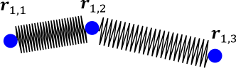
Figure 2: Isomorphism between path integrals for a single free particle in two-dimensional space and classical particles connected by springs. In the path integral interpretation, the circles and wiggly lines depict the beads and (single-particle) links of a single particle, respectively. In the classical mechanics formulation, the circles and wiggly lines depict particles and springs, respectively. The position vector of the particle is denoted by $\mathbf{r}_{1,j}$, where $j$ indicates the imaginary time index ($j=1,2$, and $3$).

In addition to the propagators $G(\mathbf{R}_{0},\mathbf{R}_{n};\tau)$ and $G(\mathbf{R}_{n},\mathbf{R}_{2n};\tau)$, the partition function contains the trial functions (or “weights”) $\psi_{T}(\mathbf{R}_{0})$ and $\psi_{T}(\mathbf{R}_{2n})$. For the single two-dimensional particle in free space, $\psi_{T}(\mathbf{r}_{0})$ and $\psi_{T}(\mathbf{r}_{2n})$ can be interpreted as potentials that are felt by the first and last particle of the chain of classical particles. Thus, we can interpret the PIGS simulation of a single particle as a simulation of a chain of classical particles connected by springs (or a polymer with nearest neighbor interactions) and two external forces that act on the particles at the ends of the chain. The stiffness of the springs is determined by $1/\Delta\tau$, i.e., by the inverse of the imaginary time step associated with the links.

The following two sections introduce two different approaches for approximating the short-time propagator, namely the Trotter formula and the pair product approximation.

3.2 Trotter formula

One way to approximate the short-time propagator is to use the Trotter formula [65]. For sufficiently small time steps $\Delta\tau$, the kinetic energy contribution $\hat{K}$ and the potential energy contribution $\hat{V}$ to the propagator can be split,

$$\exp[-\Delta\tau(\hat{K}+\hat{V})]=\exp(-\Delta\tau\hat{K})\exp(-\Delta\tau\hat{V})+\mathcal{O}(\Delta\tau^{2}),$$ (23)

where the notation $\mathcal{O}(\Delta\tau^{2})$ indicates that the leading-order error scales, in general, as $\Delta\tau$ to the power of 2. More specifically, by Taylor expanding the exponentials, one can prove that the leading-order error is $\Delta\tau^{2}[\hat{K},\hat{V}]/2$, where $[\hat{K},\hat{V}]$ is the commutator between $\hat{K}$ and $\hat{V}$, $[\hat{K},\hat{V}]=\hat{K}\hat{V}-\hat{V}\hat{K}$. In the $\Delta\tau\rightarrow 0$ limit (this corresponds to the insertion of infinitely many time slices, i.e., the $n\rightarrow\infty$ limit), the Trotter formula becomes exact. Since $n$ cannot be infinitely large in practice, one performs calculations for different $n$ and extrapolates the observables of interest to the infinite $n$ limit.

Importantly, the Trotter formula can be extended to higher orders. We can readily adopt a $\mathcal{O}(\Delta\tau^{3})$ scheme by further splitting the kinetic energy term or the potential energy term,

$$\exp[-\Delta\tau(\hat{K}+\hat{V})] =\exp(-\Delta\tau\hat{K}/2)\exp(-\Delta\tau\hat{V})\exp(-\Delta\tau\hat{K}/2)+\mathcal{O}(\Delta\tau^{3})$$ (24)

or

$$\exp[-\Delta\tau(\hat{K}+\hat{V})] =\exp(-\Delta\tau\hat{V}/2)\exp(-\Delta\tau\hat{K})\exp(-\Delta\tau\hat{V}/2)+\mathcal{O}(\Delta\tau^{3}).$$ (25)

In practice, Eq. (25), which is accurate up to second order [the error is $\mathcal{O}(\Delta\tau^{3})$], is easier to use than Eq. (24). In position space, Eq. (25) reads

$$G(\mathbf{R},\mathbf{R}^{\prime};\Delta\tau)=\exp[-\Delta\tau V(\mathbf{R})/2]\exp[-\Delta\tau V(\mathbf{R}^{\prime})/2]G_{0}(\mathbf{R},\mathbf{R}^{\prime};\Delta\tau)+\mathcal{O}(\Delta\tau^{3}),$$ (26)

where $G_{0}$ [see Eq. (16)] is the propagator that accounts for the kinetic energy term.

One can reach successively higher accuracy by the repeated use of the Baker-Campell-Hausdorff formula (see, e.g., Ref. [66])

$$e^{\epsilon\hat{A}}e^{\epsilon\hat{B}}=e^{\hat{C}},$$ (27)

where

$$\hat{C}=(\hat{A}+\hat{B})\epsilon+\frac{1}{2}[\hat{A},\hat{B}]\epsilon^{2}+\frac{1}{12}\left(\left[\hat{A},[\hat{A},\hat{B}]\right]+\left[\hat{B},[\hat{B},\hat{A}]\right]\right)\epsilon^{3}$$

$$-\frac{1}{24}\left[\hat{B},\left[\hat{A},[\hat{A},\hat{B}]\right]\right]\epsilon^{4}+\mathcal{O}(\epsilon^{5}).$$ (28)

Using Eqs. (27) and (28) twice, we obtain [67]

$$e^{\epsilon\hat{B}}e^{\epsilon\hat{A}}e^{\epsilon\hat{B}}=e^{\hat{D}},$$ (29)

where

$$\hat{D}=(\hat{A}+2\hat{B})\epsilon-\frac{1}{6}\epsilon^{3}\left[\hat{A},[\hat{B},\hat{A}]\right]+\frac{1}{6}\epsilon^{3}\left[\hat{B},[\hat{A},\hat{B}]\right]+\mathcal{O}(\epsilon^{5}).$$ (30)

Applying Eqs. (29) and (30) twice to

$$\exp\left(-\Delta\tau\frac{\hat{V}}{6}\right)\exp\left(-\Delta\tau\frac{\hat{K}}{2}\right)\exp\left(-\Delta\tau\frac{2\tilde{{V}}}{3}\right)\exp\left(-\Delta\tau\frac{\hat{K}}{2}\right)\exp\left(-\Delta\tau\frac{\hat{V}}{6}\right),$$ (31)

we can check that the fourth-order factorization [67]

$$\exp\left[-\Delta\tau(\hat{K}+\hat{V})\right]= \exp\left(-\Delta\tau\frac{\hat{V}}{6}\right)\exp\left(-\Delta\tau\frac{\hat{K}}{2}\right)\times$$

$$\exp\left(-\Delta\tau\frac{2\tilde{{V}}}{3}\right)\exp\left(-\Delta\tau\frac{\hat{K}}{2}\right)\exp\left(-\Delta\tau\frac{\hat{V}}{6}\right)$$ (32)

$$+\mathcal{O}(\Delta\tau^{5}),$$

where $\tilde{V}$ is given by $\hat{V}+\Delta\tau^{2}[\hat{V},[\hat{K},\hat{V}]]/48$, holds. The term $[\hat{V},[\hat{K},\hat{V}]]$, in position space, can be simplified to $(\hbar^{2}/m)\sum_{i=1}^{N}|\nabla_{i}V|^{2}$, where the gradient $\nabla_{i}$ in three spatial dimensions is given by

$$\nabla_{i}=\hat{x}_{i}\frac{\partial}{\partial x_{i}}+\hat{y}_{i}\frac{\partial}{\partial y_{i}}+\hat{z}_{i}\frac{\partial}{\partial z_{i}},$$ (33)

with $\hat{x}_{i}$, $\hat{y}_{i}$, and $\hat{z}_{i}$ denoting unit vectors that point in the $x_{i}$, $y_{i}$, and $z_{i}$ directions, respectively. The term $|\nabla_{i}V|^{2}$ corresponds to the square of the force on the $i$-th particle. Care needs to be taken in evaluating the derivatives, since $V$ usually contains a double sum over two-body potentials or even a triple sum over three-body potentials. In most cases, the evaluation of the force terms cannot be simplified analytically, implying that the evaluation of double commutators involves double or triple sums over the total number of particles. This makes the numerical evaluation comparatively expensive. Note that the exponentials in Eq. (32) that contain the potential energy can have different numerical factors. In addition, Eq. (32) is not the only form of the fourth-order factorization [67, 68].

Using the Trotter formula, the isomorphism between a single quantum particle in free space and the classical spring system can be extended to multiple quantum particles with interactions. Figure 3 depicts two interacting particles in two-dimensional space (it is assumed that the particles do not feel a single-particle potential).

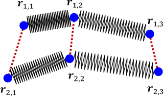
Figure 3: Isomorphism between path integrals for two interacting particles in two-dimensional space and classical particles connected by springs. In the path integral interpretation, the circles and wiggly lines depict the beads and links of a single particle, respectively, and the dotted lines depict the two-body interaction between beads with the same imaginary time index. In the classical mechanics interpretation, the circles and wiggly lines depict particles and springs, respectively, and the dotted lines depict the two-body interaction between selected classical particles. The position vector of the $k$-th particle at the $j$-th imaginary time index $j$ is denoted by $\mathbf{r}_{k,j}$.

In this case, the propagator for the link that connects the beads labeled by $\mathbf{r}_{1,j}$, $\mathbf{r}_{1,j+1}$, $\mathbf{r}_{2,j}$, and $\mathbf{r}_{2,j+1}$ reads [see Eq. (25)]

$$G(\{\mathbf{r}_{1,j},\mathbf{r}_{2,j}\},\{\mathbf{r}_{1,j+1},\mathbf{r}_{2,j+1}\};\Delta\tau)= e^{-\Delta\tau V_{\rm{2b}}(\mathbf{r}_{1,j}-\mathbf{r}_{2,j})/2}e^{-\Delta\tau V_{\rm{2b}}(\mathbf{r}_{1,j+1}-\mathbf{r}_{2,j+1})/2}$$ (34)

$$\times G_{0}(\mathbf{r}_{1,j},\mathbf{r}_{1,j+1};\Delta\tau)G_{0}(\mathbf{r}_{2,j},\mathbf{r}_{2,j+1};\Delta\tau),$$

where $V_{\rm{2b}}$ denotes the two-body interaction potential between particles 1 and 2 and $G_{0}(\mathbf{r}_{k,j},\mathbf{r}_{k,j+1};\Delta\tau)$ the single-particle propagator of the $k$-th particle [see Eq. (20)]. As in Fig. 2, two consecutive beads for the same particle (e.g., the circles labeled by $\mathbf{r}_{1,j}$ and $\mathbf{r}_{1,j+1}$ in Fig. 3) are connected by single-particle links (wiggly lines in Fig. 3) that represent the propagators $G_{0}$. Since the two-body interaction potential (dotted lines in Fig. 3) is diagonal in position space [see the exponentials on the right hand side of Eq. (34)], it connects beads of different particles with the same index, i.e., it connects $\mathbf{r}_{1,1}$ and $\mathbf{r}_{2,1}$, $\mathbf{r}_{1,2}$ and $\mathbf{r}_{2,2}$, and $\mathbf{r}_{1,3}$ and $\mathbf{r}_{2,3}$ (or, in general, it connects $\mathbf{r}_{k,j}$ and $\mathbf{r}_{k+1,j}$). Each particle in the PIGS simulation corresponds to $2n+1$ classical particles connected by springs. Classical particles associated with different chains interact only if they have the same bead index.

3.3 Pair product approximation

To introduce the pair product approximation, we assume for simplicity that the potential energy operator $\hat{V}$ can be written as a sum of two-body terms,

$$V(\mathbf{R})=\sum_{k=1}^{N-1}\sum_{l=k+1}^{N}V_{\rm{2b}}(\mathbf{r}_{k}-\mathbf{r}_{l}),$$ (35)

i.e., we assume for now that single-particle and three- and higher-body forces are absent. Under these assumptions, the short-time propagator can be evaluated using the pair product approximation [6]. It is convenient to define the two-body kinetic energy operator $\hat{K}_{kl}$ for the $k$-th and $l$-th particle in position space,

$$\hat{K}_{kl}=-\frac{\hbar^{2}}{m}\nabla_{\mathbf{r}_{k}-\mathbf{r}_{l}}^{2}.$$ (36)

The relative non-interacting and interacting two-body Hamiltonian are $\hat{K}_{kl}$ and $\hat{K}_{kl}+\hat{V}_{\rm{2b}}(\mathbf{r}_{k}-\mathbf{r}_{l})$, respectively. The pair product approximation considers two-body correlations explicitly, but not higher-body correlations, and writes the many-body propagator as a product over single-particle propagators and two-body propagators,

$$G(\mathbf{R},\mathbf{R}^{\prime};\Delta\tau)\approx G_{0}(\mathbf{R},\mathbf{R}^{\prime};\Delta\tau)\left(\prod_{k<l}^{N}\bar{G}^{\rm{rel}}(\mathbf{r}_{k}-\mathbf{r}_{l},\mathbf{r}^{\prime}_{k}-\mathbf{r}_{l}^{\prime};\Delta\tau)\right),$$ (37)

where $\bar{G}^{\rm{rel}}$,

$$\bar{G}^{\rm{rel}}(\mathbf{r}_{k}-\mathbf{r}_{l},\mathbf{r}^{\prime}_{k}-\mathbf{r}_{l}^{\prime};\Delta\tau)=\frac{\braket{\mathbf{r}_{k}-\mathbf{r}_{l}}{\exp[-\Delta\tau(\hat{K}_{kl}+\hat{V}_{\rm{2b}}(\mathbf{r}_{k}-\mathbf{r}_{l}))]}{\mathbf{r}_{k}^{\prime}-\mathbf{r}_{l}^{\prime}}}{\braket{\mathbf{r}_{k}-\mathbf{r}_{l}}{\exp(-\Delta\tau\hat{K}_{kl})}{\mathbf{r}_{k}^{\prime}-\mathbf{r}_{l}^{\prime}}},$$ (38)

is the reduced pair propagator. The denominator of the reduced pair propagator coincides with the known relative non-interacting two-body propagator. Thus the only “non-trivial input” is the relative propagator of the interacting two-body system. One can readily see that the pair product approximation is exact for two particles for any propagation time because the center-of-mass and relative degrees of freedom separate in this case. In some cases such as for the two-body zero-range interaction potential, the exact reduced pair propagator is known analytically [60, 62, 61, 63]. In other cases such as for the two-body hardcore potential, an approximate reduced pair propagator is known analytically in closed form [69, 70]. If the reduced propagator is not known analytically, one can perform a partial wave decomposition and obtain a numerical representation of the reduced two-body propagator [6].

In dilute gases or weakly-bound droplets, the interparticle spacing is typically so large that two-body collisions dominate over three- and higher-body collisions. The leading-order error of the pair product approximation is determined by the importance of three-body correlations. For two-component equal-mass Fermi gases with two-body zero-range interactions, three-body correlations are suppressed by the Pauli exclusion principle. For this system, we found that the pair product approximation provides an extremely good description of the propagator. Specifically, we obtain accurate simulation results for a small number of beads (see Sec. 5 for details). For bosons, in contrast, three-body correlations can be significant. As a consequence, the pair product approximation is not as efficient as for two-component fermions and simulations typically employ a large number of beads (“large” in this context means about two orders of magnitude more number of beads as in the simulations for fermions [45]).

To illustrate the pair product approximation, we cannot use the classical isomorphism because the kinetic and potential energy contributions are mixed. One needs to evaluate the single-particle propagator, which can be represented by springs as in Figs. 2 and 3. However, one also needs to evaluate the reduced two-body propagator, which connects two consecutive beads of one particle’s path with the same consecutive beads of another particle’s path. These “four-bead connections” do not have a simple classical analog.

3.4 Comparison of the two approximations

This section discusses the advantages and disadvantages of approximating the short-time propagator with the help of the Trotter formula and the pair product approximation.

In the Trotter formula based scheme, the kinetic and the potential energy terms are treated separately. Inserting the identity $\int_{\mathbf{R}}\ket{\mathbf{R}}\bra{\mathbf{R}}d\mathbf{R}=\hat{1}$, Eq. (8), multiple times into Eqs. (25) or (32), it can be seen that the potential energy is diagonal in position space. This means that one can directly evaluate the potential energy term at each time slice. The kinetic energy term contains off-diagonal terms and needs to be evaluated at each link instead of at each time slice. Nevertheless, since the kinetic energy term corresponds to a simple Gaussian, the sampling of the kinetic energy piece of the propagator can, in general, be performed efficiently (see Sec. 4.3.2 for details).

Even though the Trotter formula can formally be generalized to expressions that are accurate to order $\Delta\tau^{5},\Delta\tau^{6},\cdots$ [71, 72], many of these expressions are of limited use in practice because they contain either commutators that involve rather complicated expressions or terms that correspond to negative imaginary time, which are not normalizable. There exists a multi-product expansion for the propagator [72]; however, applications thereof are still rare [73]. Thus present-day algorithms mostly employ Trotter formula based decompositions that are accurate to order $\Delta\tau^{4}$.

In the pair product approximation, the two-body reduced propagator contains kinetic energy and potential energy contributions. This means that the reduced two-body propagator has to be evaluated at each link. Because the reduced two-body propagator is, in general, not a simple Gaussian, the sampling is typically less efficient than in the case where the Trotter formula is used. Furthermore, as discussed in Sec. 4.6, the evaluation of the permutations is computationally more involved.

Our discussion of the pair product approximation assumed that the potential energy can be written as a sum over two-body terms. If the Hamiltonian contains one-, three-, or higher-body potential energy terms, one can include them by combining the Trotter formula and the pair product approximation. To this end, one first splits the propagator into two terms using the Trotter formula. The first term contains the kinetic energy operator and the two-body interactions while the second term contains all other potential terms. One then applies the pair product approximation to the first term. In this approach, it is most convenient to use the second-order Trotter formula for two reasons. First, if a higher-order Trotter formula was used, one would need to evaluate the commutator between the one-, three- and higher-body potential terms and the two-body potential terms. For the two-body zero-range interactions considered in Sec. 5 this is a rather challenging task. Second, both the second-order Trotter formula and the pair product approximation yield errors for the energy that scale quadratically with the time step $\Delta\tau$. While the error in the pair product approximation tends to be smaller than that associated with the pair product approximation, ultimately it is the scaling with $\Delta\tau$ that determines the accuracy and use of the fourth-order Trotter formula typically leads only to a small overall improvement.

From our perspective, the pair product approximation has one key advantage: It can deal with a class of two-body potentials that the Trotter formula based scheme cannot deal with (at least no such treatment is known to us). For example, the two-body hardcore and zero-range potentials contain infinities and can thus not be treated by the Trotter formula based scheme. However, the infinities can, as discussed in the next section exemplarily for the two-body zero-range potential, be dealt with analytically in the pair product approximation.

3.5 Propagator for two-body zero-range interactions

As alluded to in the previous section, two-body zero-range interactions can be incorporated into continuum Monte Carlo simulations through the pair product approximation [45, 42, 44, 46], which employs the relative propagator $\bar{G}^{\rm{rel}}$ [see Eqs. (37) and (38)]. In what follows, we limit our discussion to three spatial dimensions. To determine $\bar{G}^{\rm{rel}}$, one considers the relative Hamiltonian $H^{\rm{rel}}$ for two particles interacting through the regularized zero-range Fermi-Huang pseudopotential $V_{\rm{F}}(r)$ [74] in free space,

$$H^{\rm{rel}}=-\frac{\hbar^{2}}{2\mu}\nabla_{\mathbf{r}}^{2}+V_{\rm{F}}(r),$$ (39)

where

$$V_{\rm{F}}(r)=\frac{2\pi\hbar^{2}a_{s}}{\mu}\delta^{(3)}(\mathbf{r})\frac{\partial}{\partial r}r.$$ (40)

Here, $\mu$ denotes the two-body reduced mass, $\mathbf{r}$ the interparticle distance vector, and $a_{s}$ the $s$-wave scattering length. The regularization operator $(\partial/\partial r)r$ in Eq. (40) ensures that the Hamiltonian is well-behaved. Without this operator, the two-body coupling constant would have to be renormalized. With the regulator, however, the coupling strength is uniquely determined and given by $2\pi\hbar^{2}a_{s}/\mu$.

The reduced (or normalized) relative propagator corresponding to the Hamiltonian given in Eq. (39) reads [61, 63]

$$\bar{G}^{\rm{rel}}(\mathbf{r},\mathbf{r}^{\prime};\tau)=1+\frac{\hbar^{2}\tau}{\mu rr^{\prime}}\exp\left(-\frac{\mu rr^{\prime}(1+\cos\theta)}{\hbar^{2}\tau}\right)\left(1+\frac{\hbar}{a_{s}}\sqrt{\frac{\pi\tau}{2\mu}}{\rm{erfc}}(v)\exp(v^{2})\right),$$ (41)

where $\cos\theta=\mathbf{r}\cdot\mathbf{r}^{\prime}/(rr^{\prime})$ and $v=[r+r^{\prime}-\tau\hbar^{2}/(\mu a_{s})]/\sqrt{2\tau\hbar^{2}/\mu}$. For $|a_{s}|=\infty$, the length scale $a_{s}$ drops out of the expression for the propagator and Eq. (41) simplifies to

$$\bar{G}^{\rm{rel}}(\mathbf{r},\mathbf{r}^{\prime};\tau)=1+\frac{\hbar^{2}\tau}{\mu rr^{\prime}}\exp\left(-\frac{\mu rr^{\prime}(1+\cos\theta)}{\hbar^{2}\tau}\right).$$ (42)

Importantly, the reduced relative propagator diverges when $r$ or $r^{\prime}$ approach zero. These divergencies have implications for the Monte Carlo sampling of the paths. As discussed in detail in Sec. 4.3.3, moves have to be designed carefully such that detailed balance is fulfilled. For example, while $\bar{G}^{\rm{rel}}$ diverges for $r$ and $r^{\prime}\rightarrow 0$, the probability to find two particles at vanishing interparticle distance does not diverge. The treatment of systems with two-body hardcore interactions is similar in spirit to that detailed here for two-body zero-range interactions.

Adding the spherically symmetric harmonic confining potential $V_{\rm{trap}}(r)=\mu\omega^{2}r^{2}/2$ for the relative degrees of freedom to the Hamiltonian $H^{\rm{rel}}$ given in Eq. (39) and assuming that $a_{s}$ is infinitely large, the reduced relative propagator $\bar{G}^{\rm{rel}}(\mathbf{r},\mathbf{r}^{\prime};\tau)$ reads

$$\bar{G}^{\rm{rel}}(\mathbf{r},\mathbf{r}^{\prime};\tau)=1+\frac{2a_{\rm{ho}}^{2}}{rr^{\prime}}\mbox{sinh}(\tau\hbar\omega)\exp\left(-\frac{rr^{\prime}(1+\cos\theta)}{2a_{\rm{ho}}^{2}{\rm{sinh}}(\tau\hbar\omega)}\right),$$ (43)

where $a_{\rm{ho}}=\sqrt{\hbar/(m\omega)}$. In the limit that the angular trapping frequency $\omega$ goes to zero, Eq. (43) reduces to Eq. (42). Expression (43) is used in Sec. 5 to treat harmonically trapped two-component Fermi gases with two-body zero-range interactions at unitarity using the pair product approximation.

4 Monte Carlo techniques and the PIGS algorithm

Throughout this section we assume that the trial function $\psi_{T}(\mathbf{R})$ is given and that its value can be determined for any set of coordinates $\mathbf{R}$. The functional form of $\psi_{T}(\mathbf{R})$ depends sensitively on the system under study. The choice of $\psi_{T}(\mathbf{R})$ and the dependence of the PIGS results on $\psi_{T}(\mathbf{R})$ will be discussed in Sec. 5 for harmonically trapped two-component Fermi gases.

4.1 General sampling scheme: Importance sampling

Equation (19) writes the long-time propagator as a high-dimensional integral over a product of short-time propagators. This implies that the evaluation of the normalization factor $Z(\tau)$ is a high-dimensional integral. This section discusses the Monte Carlo sampling of this high-dimensional integral over $\{\mathbf{R}_{0},\cdots,\mathbf{R}_{2n}\}$ (there are $3\times(2n+1)\times N$ independent coordinates if we are considering three spatial dimensions). To proceed, we write $Z(\tau)$ explicitly in terms of the short-time propagator,

$$Z(\tau)=\int_{\mathbf{R}_{0}}\cdots\int_{\mathbf{R}_{2n}}\pi(\mathbf{R}_{0},\cdots,\mathbf{R}_{2n})d\mathbf{R}_{0}\cdots d\mathbf{R}_{2n},$$ (44)

where

$$\pi(\mathbf{R}_{0},\cdots,\mathbf{R}_{2n})= \psi_{T}(\mathbf{R}_{0})G(\mathbf{R}_{0},\mathbf{R}_{1};\Delta\tau)G(\mathbf{R}_{1},\mathbf{R}_{2};\Delta\tau)$$ (45)

$$\times\cdots\times G(\mathbf{R}_{2n-1},\mathbf{R}_{2n};\Delta\tau)\psi_{T}(\mathbf{R}_{2n}).$$

To simplify the notation, we denote the configuration $\{\mathbf{R}_{0},\cdots,\mathbf{R}_{2n}\}$ by $\mathbf{x}$ and the probability distribution $\pi(\mathbf{R}_{0},\cdots,\mathbf{R}_{2n})$ by $\pi(\mathbf{x})$. The notation of these and other quantities is summarized in Tables 1 and 2.

Table 2: Definitions of Monte Carlo sampling terminology used in this article. Columns 1-3 show the symbol, name, and related equation number, respectively. The configuration $\mathbf{x}$ is defined as $\mathbf{x}=\{\mathbf{R}_{0},\cdots,\mathbf{R}_{2n}\}$.

$\pi(\mathbf{x})$	probability distribution	Eq. (45)
$p(\mathbf{x})$	probability density function	Eq. (48)
$w(\mathbf{x})$	weight function (observable specific)	Eqs. (46)-(47); Sec. 4.4
$P(\mathbf{x}\to\mathbf{x}^{\prime})$	transition probability	Eq. (49)
$\cal{G}(\mathbf{x}\to\mathbf{x}^{\prime})$	proposal distribution (selected by simulator)	around Eqs. (49)-(50)
$\cal{A}(\mathbf{x}\to\mathbf{x}^{\prime})$	acceptance distribution	Eq. (50)
$\psi_{T}(\mathbf{R})$	trial function (selected by simulator)	Eq. (1)

The expectation value $\braket{{O}}$ of an arbitrary observable ${O}$ can be written as

$$\braket{{O}}=\frac{\int_{\mathbf{x}}w(\mathbf{x})\pi(\mathbf{x})d\mathbf{x}}{\int_{\mathbf{x}}\pi(\mathbf{x})d\mathbf{x}},$$ (46)

where the integration goes over $3\times(2n+1)\times N$ coordinates and the weight function $w(\mathbf{x})$ needs to be determined, as will be discussed in Sec. 4.4, for each observable. To see the structure of $\braket{{O}}$ more clearly, we rewrite Eq. (46) as

$$\braket{{O}}=\int_{\mathbf{x}}w(\mathbf{x})p(\mathbf{x})d\mathbf{x},$$ (47)

where the probability density function $p(\mathbf{x})$ is defined as

$$p(\mathbf{x})=\frac{\pi(\mathbf{x})}{\int_{\mathbf{x}^{\prime}}\pi(\mathbf{x}^{\prime})d\mathbf{x}^{\prime}}.$$ (48)

In contrast to the probability distribution $\pi(\mathbf{x})$, the probability density function $p(\mathbf{x})$ is normalized; $w(\mathbf{x})$ and $p(\mathbf{x})$ represent the weight contributed to the observable by the configuration $\mathbf{x}$ and the normalized probability to be in the configuration $\mathbf{x}$, respectively. Equation (47) provides the basis of importance sampling: Configurations are not blindly distributed uniformly in space but instead are distributed according to $p(\mathbf{x})$. The advantage of importance sampling is that most computer time is used to sample configurations that are physically relevant and little time to sample configurations that do not contribute significantly to $\braket{{O}}$.

The general idea of the PIGS algorithm is to generate configurations $\mathbf{x}$ according to $p(\mathbf{x)}$ and to use the generated configurations to accumulate the weight functions $w(\mathbf{x})$ for a set of observables. Thus, it is crucial to have correct and efficient sampling schemes that explore the full configuration space with a relatively high acceptance ratio and without getting stuck around a local minimum. Section 4.2 reviews the basics of selected Monte Carlo methods, which are then used in the subsequent sections.

4.2 Some background on Monte Carlo methods

This section discusses how to update or generate configurations using the Metropolis algorithm. A Markov process is uniquely defined by the transition probability $P(\mathbf{x}\to\mathbf{x}^{\prime})$ to go from configuration $\mathbf{x}$ to configuration $\mathbf{x}^{\prime}$. The Metropolis algorithm satisfies the detailed balance condition [7]

$$\pi(\mathbf{x})P(\mathbf{x}\to\mathbf{x}^{\prime})=\pi(\mathbf{x}^{\prime})P(\mathbf{x}^{\prime}\to\mathbf{x}),$$ (49)

which states that the flow of probability from $\mathbf{x}$ to $\mathbf{x}^{\prime}$ is equal to that from $\mathbf{x}^{\prime}$ to $\mathbf{x}$. This means that there is no net flow of probability. The Metropolis algorithm needs to ensure ergodicity of the Markov process. If the process is ergodic, the Markov chain (i) returns to any previously generated configuration $\mathbf{x}$ after a sufficiently long simulation time and (ii) is not periodic (a Markov chain of $\{\mathbf{x},\mathbf{x}^{\prime},\mathbf{x},\mathbf{x}^{\prime},\cdots\}$, e.g., is periodic). The ergodicity ensures that the probability distribution $\pi(\mathbf{x})$ gets sampled fully. For example, as discussed in Ref. [75], if we use the traditional scheme of treating the permutations [6], for a two-component Fermi gas with zero-range interactions, the Markov process ends up with a configuration in which all particles sit on top of each other and the configuration never returns to the original configuration $\mathbf{x}$. This means that ergodicity is violated and that the Markov process does not generate samples according to $p(\mathbf{x})$. This renders the sampled configurations meaningless. We note, however, that while the detailed balance condition together with the ergodicity guarantees that the equilibrium distribution coincides with the desired probability distribution $\pi(\mathbf{x})$, there exist other Monte Carlo methods that do not satisfy the detailed balance condition but yield an equilibrium distribution that coincides with the desired probability distribution $\pi(\mathbf{x})$ [76].

The Metropolis algorithm consists of two steps [7]: (i) the generation of a proposed configuration (or move) and (ii) the acceptance or rejection of the proposed configuration (or move). The combination of (i) and (ii) leads to a new configuration. Starting from the configuration $\mathbf{x}$, we propose a new configuration $\mathbf{x}^{\prime}$ according to a proposal distribution $\cal{G}(\mathbf{x}\to\mathbf{x}^{\prime})$ and accept (the new configuration would be $\mathbf{x}^{\prime}$) or reject the new configuration (the new configuration would be $\mathbf{x}$) according to the acceptance distribution ${\cal{A}}(\mathbf{x}\to\mathbf{x}^{\prime})$. This implies that $P(\mathbf{x}\rightarrow\mathbf{x}^{\prime})$ is given by $\cal{G}(\mathbf{x}\to\mathbf{x}^{\prime}){\cal{A}}(\mathbf{x}\to\mathbf{x}^{\prime})$. The Metropolis algorithm chooses ${\cal{A}}(\mathbf{x}\to\mathbf{x}^{\prime})$ such that [7]

$${\cal{A}}(\mathbf{x}\to\mathbf{x}^{\prime})=\min\left(1,\frac{\pi(\mathbf{x}^{\prime})\cal{G}(\mathbf{x}^{\prime}\to\mathbf{x})}{\pi(\mathbf{x})\cal{G}(\mathbf{x}\to\mathbf{x}^{\prime})}\right).$$ (50)

We verify that the detailed balance condition [Eq. (49)] is satisfied in the following. If $\pi(\mathbf{x}^{\prime})\cal{G}(\mathbf{x}^{\prime}\to\mathbf{x})$ is smaller than $\pi(\mathbf{x})\cal{G}(\mathbf{x}\to\mathbf{x}^{\prime})$, we obtain from Eq. (50) that

$$P(\mathbf{x}\to\mathbf{x}^{\prime})=\frac{\pi(\mathbf{x}^{\prime})\cal{G}(\mathbf{x}^{\prime}\to\mathbf{x})}{\pi(\mathbf{x})}$$ (51)

and

$$P(\mathbf{x}^{\prime}\to\mathbf{x})=\cal{G}(\mathbf{x}^{\prime}\to\mathbf{x}).$$ (52)

Plugging the right-hand sides of Eqs. (51) and (52) into Eq. (49), we confirm that Eq. (49) holds. If $\pi(\mathbf{x}^{\prime})\cal{G}(\mathbf{x}^{\prime}\to\mathbf{x})$ is larger or equal to $\pi(\mathbf{x})\cal{G}(\mathbf{x}\to\mathbf{x}^{\prime})$, it can be checked similarly that Eq. (49) holds. Thus, we have shown that detailed balance is fulfilled.

A key task is to design proposal distributions ${\cal{G}}(\mathbf{x}\to\mathbf{x}^{\prime})$ that ensure the complete and, ideally, efficient exploration of the entire configuration space. In most cases, efficient simulation schemes are achieved if more than one proposal distribution (and hence type of move) is utilized. As discussed more in the next section, the proposal distribution might be designed based on the knowledge of the non-interacting system (see, e.g., Sec. 4.3.2) or based on knowledge of certain limiting behaviors of the interacting system (see, e.g., Sec. 4.3.3).

In practice, the acceptance ratio $A$, i.e., one minus the fraction of rejected moves, should be monitored (note, $A$ is a number and not an $\mathbf{x}$- and $\mathbf{x}^{\prime}$-dependent function). The acceptance ratio $A$ for Metropolis sampling is different from the acceptance ratio encountered in the rejection sampling. In the rejection sampling, a rejected configuration does not lead to a new configuration. In the Metropolis sampling, in contrast, a rejected configuration does lead to a new configuration. When a configuration is rejected, the old configuration becomes the new configuration. For most of the updates (i.e., the generation of proposed new configurations), the acceptance ratio should not be too large and not be too small. A high acceptance ratio typically implies that the deviation between the old and new configurations is, on average, small. This means that the configuration space is explored comparatively slowly. A low acceptance ratio, in contrast, means that the Markov chain contains many identical configurations; again, typically this means that the configuration space is explored comparatively slowly. Both cases can result in large correlations of the sample and should be avoided. As a rule of thumb, the acceptance ratio should lie roughly between 30% and 50% [77].

4.3 Moves

The previous section outlined the basics of the Metropolis algorithm. This section discusses the PIGS moves that are used to update the configurations. For all moves, the proposed new configuration $\mathbf{x}^{\prime}$ is chosen based on the proposal distribution ${\cal{G}}(\mathbf{x}\to\mathbf{x}^{\prime})$ and accepted/rejected based on the acceptance distribution ${\cal{A}}(\mathbf{x}\to\mathbf{x}^{\prime})$. Once ${\cal{G}}(\mathbf{x}\to\mathbf{x}^{\prime})$ is specified, ${\cal{A}}(\mathbf{x}\to\mathbf{x}^{\prime})$ follows from Eq. (50). This section discusses three different moves. The “naive move” and the “wiggle move” are “all purpose” moves, which have proven to be useful for nearly all systems. In some cases, the use of these two types of moves alone does not lead to an efficient (or even correct) exploration of the configuration space. For systems with two-body zero-range interactions, e.g., the “pair distance move” is needed. In general, the simulator decides on the frequency with which the individual moves are used. The optimal ratio can be found empirically from the performance of the simulation itself or through the implementation of some sort of learning algorithm.

The list of moves discussed below does not include a “permutation move”, i.e., the stochastic sampling of the permutations is not discussed. The reason for this is twofold. If the system contains identical bosons, the ground state wave function is typically identical to that of Boltzmann particles, eliminating the need for an explicit symmetrization. If the system contains identical fermions, we employ the on-the-fly anti-symmetrization scheme discussed in Sec. 4.6, which is particularly useful if two-body zero-range interactions are employed.

The moves employed in the PIGS algorithm have much in common with the moves employed in the finite-temperature path integral Monte Carlo algorithm. As already discussed, one difference is that the PIGS algorithm contains the trial function $\psi_{T}$ while the finite-temperature path integral Monte Carlo algorithm does not. Quite generally, whether a move depends on the trial function $\psi_{T}$ or not depends on whether or not the beginning time slice $\mathbf{R}_{0}$ or the ending time slice $\mathbf{R}_{2n}$ are being updated. In the implementations of the moves discussed below, the wiggle move does not depend on $\psi_{T}$, and the naive move and the pair move may depend on $\psi_{T}$ (it depends on whether or not the randomly selected time slice to be updated is the $0$-th or $2n$-th time slice). It should be noted, though, that the moves can, in principle, be implemented in a variety of ways, i.e., slightly different proposal distributions ${\cal{G}}(\mathbf{x}\to\mathbf{x}^{\prime})$ might be used in different implementations and be referred to by the same move name.

4.3.1 Naive move

The simplest move (the naive move) consists of shifting the position vector $\mathbf{r}_{\rm{old}}$ of a single bead by $\delta\mathbf{r}$, where $\delta\mathbf{r}$ is drawn uniformly from the interval $[-\Delta\mathbf{r},\Delta\mathbf{r}]$. The basic idea behind this move is that the propagator is a smooth function of $\mathbf{x}$ and that a small change in $\mathbf{x}$ does not introduce a huge change in the probability distribution $\pi(\mathbf{x})$. The size $2\Delta\mathbf{r}$ of the interval (if we are simulating a three-dimensional system, then the interval corresponds to a cube) can be adjusted such that the acceptance ratio of the proposed new position vector is around 50%. The proposal distribution $\cal{G}(\mathbf{x}\to\mathbf{x}^{\prime})$ is equal to a constant if the new bead lies in the interval $[\mathbf{r}_{\rm{old}}-\Delta\mathbf{r},\mathbf{r}_{\rm{old}}+\Delta\mathbf{r}]$; otherwise, ${\cal{G}}(\mathbf{x}\to\mathbf{x}^{\prime})$ is equal to $0$. Following Eq. (50), the move is accepted according to

$${\cal{A}}(\mathbf{x}\to\mathbf{x}^{\prime})=\min\left(1,\frac{\pi(\mathbf{x}^{\prime})}{\pi(\mathbf{x})}\right).$$ (53)

Importantly, one cannot choose an “unbalanced” interval like $[-\epsilon\Delta\mathbf{r},\Delta\mathbf{r}]$, where $\epsilon<1$, since the detailed balance condition, Eq. (49), is not satisfied in this case. The reason is that it is possible to go from $\mathbf{r}$ to $\mathbf{r}+\Delta\mathbf{r}$ in one move but that it is impossible to go from $\mathbf{r}+\Delta\mathbf{r}$ to $\mathbf{r}$ in one move.

The algorithm for the naive move can be summarized as follows. (i) Let the current configuration be $\mathbf{x}=\{\mathbf{R}_{0},\cdots,\mathbf{R}_{2n}\}$. Randomly select a particle index $k$ and a time slice index $j$, where $j$ can take any value from $0$ to $2n$. Set $\mathbf{r}_{\rm{old}}=\mathbf{r}_{k,j}$ and calculate the old probability distribution $\pi_{\rm{old}}=\pi(\mathbf{R}_{0},\cdots,\mathbf{R}_{2n})$. (ii) Generate a new position $\mathbf{r}_{\rm{new}}=\mathbf{r}_{\rm{old}}+\delta{\mathbf{r}}$, where $\delta{\mathbf{r}}$ is drawn uniformly from the interval $[-\Delta\mathbf{r},\Delta\mathbf{r}]$. Define $\mathbf{R}_{j}^{\rm{new}}=\{\mathbf{r}_{1,j},\cdots,\mathbf{r}_{k-1,j},\mathbf{r}_{\rm{new}},\mathbf{r}_{k+1,j},\cdots,\mathbf{r}_{N,j}\}$ and calculate the new probability distribution $\pi_{\rm{new}}=\pi(\mathbf{R}_{0},\cdots\mathbf{R}_{j-1},\mathbf{R}_{j}^{\rm{new}},\mathbf{R}_{j+1},\cdots,\mathbf{R}_{2n})$. (iii) Calculate the ratio $\pi_{\rm{new}}/\pi_{\rm{old}}$. If this ratio is larger than a random number drawn uniformly from 0 to 1, accept the move and set $\mathbf{r}_{k,j}=\mathbf{r}_{\rm{new}}$; otherwise, reject the move and set $\mathbf{r}_{k,j}=\mathbf{r}_{\rm{old}}$ (i.e., do not change $\mathbf{r}_{k,j}$). Figure 4 illustrates the naive move for a single particle in a one-dimensional harmonic trap. It can be seen that the proposed move involves only one bead.

Although the naive move attemps to change only one bead at a time, whether the proposed move gets accepted or rejected depends, in principle, on all the beads, i.e., the coordinates of all particles at all time slices, since the acceptance/rejection depends on the ratio $\pi_{\rm{new}}/\pi_{\rm{old}}$. However, because the probability distribution $\pi(\mathbf{x})$ is a product over propagators and the trial function $\psi_{T}$ evaluated at the two ends [Eq. (45)], the only terms that contribute to the ratio $\pi_{\rm{new}}/\pi_{\rm{old}}$ are the propagators $G(\mathbf{R}_{j-1},\mathbf{R}_{j};\Delta\tau)$ and $G(\mathbf{R}_{j},\mathbf{R}_{j+1};\Delta\tau)$ and, if $j$ equals $0$ or $2n$, the trial function $\psi_{T}(\mathbf{R}_{0})$ or $\psi_{T}(\mathbf{R}_{2n})$. If one uses the second-order Trotter formula [Eq. (26)], which treats the potential and kinetic energy terms separately, the terms that contribute to $G(\mathbf{R}_{j-1},\mathbf{R}_{j};\Delta\tau)$ and $G(\mathbf{R}_{j},\mathbf{R}_{j+1};\Delta\tau)$ are the potential energy term $\exp[-\Delta\tau V(\mathbf{R}_{j})]$ and the kinetic energy terms $G_{0}(\mathbf{r}_{k,j-1},\mathbf{r}_{k,j};\Delta\tau)$ and $G_{0}(\mathbf{r}_{k,j},\mathbf{r}_{k,j+1};\Delta\tau)$.

The caveat of the naive move is that the correlation length is typically large. In the best case scenario (i.e., in the case where all beads of all particles are considered exactly once and all proposed moves are accepted), $(2n+1)\times N$ moves are needed to generate a configuration in which every bead differs from the starting configuration. Thus, we calculate observables for every $(\alpha\times(2n+1)\times N)$-th configuration, where $\alpha$ is a constant greater than 1 that is adjusted to ensure that the observables are calculated from configurations with small correlations. In practice, we find that $\alpha$ lies between 2 and 20 for the applications considered in this review.

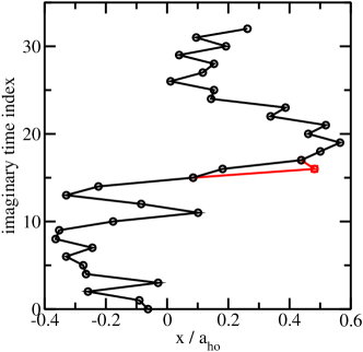
Figure 4: Illustration of the naive move for a single particle in a one-dimensional harmonic trap for $n=32$ beads. The black circles depict the old bead positions. The red square shows the proposed bead position for the 16-th time slice index. It can be seen that only two links (namely the link involving the 15-th and 16-th beads and that involving the 16-th and 17-th beads) are changed.

4.3.2 Wiggle move

The wiggle move uses the non-interacting propagator to design the proposal distribution ${\cal{G}}(\mathbf{x}\to\mathbf{x}^{\prime})$. Since the non-interacting propagator is a product of simple Gaussians for particles in free space [Eq. (16)] and for particles confined in a harmonic trap [59, 45], one can generate configurations efficiently with 100 % acceptance ratio using the Box-Muller transformation [78] or with finite acceptance ratio using the Marsaglia polar method (the acceptance ratio is around 80 %) [79] or the Ziggurat algorithm (the acceptance ratio is around 98 %) [80, 81]. If the difference between the propagator of the system to be simulated and the non-interacting propagator is small, the acceptance ratio for a move generated based on the propagator of the non-interacting system is high. Despite the large acceptance ratio, the correlation between consecutive configurations is, in general, small. In the non-interacting limit, the acceptance ratio is exactly 1.

Depending on the number of beads changed simultaneously, the wiggle move is a single-bead move or a multi-bead move. The single-bead version of the wiggle move randomly selects a particle index $k$ and a time slice index $j$ ($j>0$ and $j<2n$). Since the beads to be moved exclude the time slices $0$ and $2n$, the wiggle move does not involve the trial function $\psi_{T}$. We denote the new proposed position vector by $\mathbf{r}_{k,j}^{\rm{new}}$ (how to choose $\mathbf{r}_{k,j}^{\rm{new}}$ is discussed below) and define $\mathbf{R}_{j}^{\rm{new}}=(\mathbf{r}_{1,j},\cdots,\mathbf{r}_{k-1,j},\mathbf{r}_{k,j}^{\rm{new}},\mathbf{r}_{k+1,j},\cdots,\mathbf{r}_{N,j})$. The old and proposed configurations read

$$\mathbf{x}=\{\mathbf{R}_{0},\cdots,\mathbf{R}_{2n}\}$$ (54)

and

$$\mathbf{x}^{\prime}=\{\mathbf{R}_{0},\cdots\mathbf{R}_{j-1},\mathbf{R}_{j}^{\rm{new}},\mathbf{R}_{j+1},\cdots,\mathbf{R}_{2n}\},$$ (55)

respectively. We choose ${\cal{G}}(\mathbf{x}\to\mathbf{x}^{\prime})$ according to the propagator $G_{0}$ [Eq. (16)] of the non-interacting system without confinement (the proposal distribution based on the propagator of the non-interacting harmonic oscillator Hamiltonian can be treated similarly),

$${\cal{G}}(\mathbf{x}\to\mathbf{x}^{\prime})=\exp\left(-\frac{(\mathbf{r}_{k,j}^{\rm{new}}-\mathbf{r}_{k,j-1})^{2}+(\mathbf{r}_{k,j}^{\rm{new}}-\mathbf{r}_{k,j+1})^{2}}{4\lambda_{m}\Delta\tau}\right)$$ (56)

or, rearranging the exponent,

$${\cal{G}}(\mathbf{x}\to\mathbf{x}^{\prime})=\exp\left(-\frac{[\mathbf{r}_{k,j}^{\rm{new}}-(\mathbf{r}_{k,j-1}+\mathbf{r}_{k,j+1})/2]^{2}}{2\lambda_{m}\Delta\tau}\right).$$ (57)

The right hand side of Eq. (57) is equal to a Gaussian whose mean value is given by the midpoint of the $(j-1)$-th and the $(j+1)$-th bead of the $k$-th particle and whose variance is $\lambda_{m}\Delta\tau$. Thus, $\mathbf{r}_{k,j}^{\rm{new}}$ can be generated using the Box-Muller transformation, the Marsaglia polar method, or the Ziggurat algorithm discussed above. If we use the second-order Trotter formula, the acceptance probability ${\cal{A}}(\mathbf{x}\to\mathbf{x}^{\prime})$ [Eq. (50)] takes a fairly simple form since a large number of terms (those not involving time slice $j$ and those not involving particle $k$) in the ratio $\pi(\mathbf{x^{\prime}})/\pi(\mathbf{x})$ can be cancelled. If the pair product approximation is used, the evaluation of ${\cal{A}}(\mathbf{x}\to\mathbf{x}^{\prime})$ is more involved since fewer terms in the ratio $\pi(\mathbf{x^{\prime}})/\pi(\mathbf{x})$ can be cancelled due to the fact that the kinetic energy and the potential energy terms are “linked” in the pair product approximation.

The single-bead version of the wiggle move can be generalized to multiple consecutive beads. Since the multi-bead move leads to a deformation of a segment of the path, the move is called “wiggle move”. In what follows, our discussion is guided by Ref. [9]. Instead of a single bead of the path we propose to change a path segment consisting of multiple beads according to a proposal distribution ${\cal{G}}(\mathbf{x}\to\mathbf{x}^{\prime})$ that generalizes the expression given in Eq. (57). We denote the time slice indices of the two ends that are unchanged by $j$ and $j+s$, where $s$ is an integer power of 2; the condition for $s$ allows one, as will become clear below, to organize the move into “levels”. The corresponding position vectors are $\mathbf{r}_{k,j}$ and $\mathbf{r}_{k,j+s}$, where $s>0$. Note that the wiggle move does not explicitly involve the trial function $\psi_{T}$ since the path segment to be changed has to be continuous. This means that the zeroth bead can be at the beginning of the segment but nowhere else and that the $2n$-th bead can be at the end of the segment but nowhere else. In the finite-temperature path integral Monte Carlo approach, in contrast, any path segment can be considered, provided the path is closed.

We now outline the multi-bead move, both without and with “staging”. The algorithm without staging is less efficient but can be employed in connection with the Trotter formula and the pair product approximation. The staging version can only be used in connection with the Trotter formula. Both multi-bead move versions generate a proposed new path segment $\{\mathbf{r}_{k,j+1}^{\rm{new}},\cdots,\mathbf{r}_{k,j+s-1}^{\rm{new}}\}$ that is completely independent of the old path segment $\{\mathbf{r}_{k,j+1},\cdots,\mathbf{r}_{k,j+s-1}\}$. Here, $j+s$ has to be smaller than or equal to $2n$.

To motivate the strategy of the multi-bead wiggle move, we write the pieces of the non-interacting propagator $G_{0}$ that depend on the particle index $k$ and the time slice indices $j$ to $j+s$ out explicitly,

$$G_{0}\sim \underbrace{\exp\left[-\frac{(\mathbf{r}_{k,j}-\mathbf{r}_{k,j+s})^{2}}{4s\lambda_{m}\Delta\tau}\right]}_{\rm{constant}}\times$$ (58)

$$\underbrace{\exp\left[-\frac{(\mathbf{r}_{k,j+s/2}-\bar{\mathbf{r}}_{k,j,j+s})^{2}}{s\lambda_{m}\Delta\tau}\right]}_{\rm{zerothlevel}}\times$$

$$\underbrace{\exp\left[-\frac{(\mathbf{r}_{k,j+s/4}-\bar{\mathbf{r}}_{k,j,j+s/2})^{2}}{s\lambda_{m}\Delta\tau/2}\right]\exp\left[-\frac{(\mathbf{r}_{k,j+3s/4}-\bar{\mathbf{r}}_{k,j+s/2,j+s})^{2}}{s\lambda_{m}\Delta\tau/2}\right]}_{\rm{firstlevel}}\times$$

$$\dots,$$

where $\bar{\mathbf{r}}_{k,\alpha,\beta}=(\mathbf{r}_{k,\alpha}+\mathbf{r}_{k,\beta})/2$. If $s$ is equal to $2^{l}$, Eq. (58) contains $l$ levels (the zeroth level is counted as one level but the constant term is not). Equation (58) suggests that the sampling can be done level by level. For example, for a path segment consisting of three time slices ($s=4$ and $j=0$), the beginning bead is $\mathbf{r}_{k,0}$ and the ending bead is $\mathbf{r}_{k,4}$. Thus, there exist two levels in total. First, the new midpoint bead $\mathbf{r}_{k,2}^{\rm{new}}$ is proposed according to the $0$-th level (partial) proposal distribution ${\cal{G}}_{0-{\rm{th}}}(\mathbf{x}\to\mathbf{x}^{\prime})$, i.e., $\mathbf{r}_{k,2}^{\rm{new}}$ is generated by sampling a three-dimensional Gaussian distribution with variance $s\lambda_{m}\Delta\tau/2$. Second, the new midpoint beads $\mathbf{r}_{k,1}^{\rm{new}}$ and $\mathbf{r}_{k,3}^{\rm{new}}$ are proposed according to the $1$-st level (partial) proposal distribution ${\cal{G}}_{1-{\rm{st}}}(\mathbf{x}\to\mathbf{x}^{\prime})$, i.e., $\mathbf{r}_{k,1}^{\rm{new}}$ and $\mathbf{r}_{k,3}^{\rm{new}}$ are generated by sampling three-dimensional Gaussian distributions with variance $s\lambda_{m}\Delta\tau/4$.

In general, the $u$-th level (partial) proposal distribution ${\cal{G}}_{u-{\rm{th}}}(\mathbf{x}\to\mathbf{x}^{\prime})$ reads

$${\cal{G}}_{u-{\rm{th}}}(\mathbf{x}\to\mathbf{x}^{\prime})=$$

$$\prod_{v=1}^{2^{u}}\exp\left(-\frac{[\mathbf{r}_{k,j+s(2v-1)/2^{u+1}}^{\rm{new}}-(\mathbf{r}_{k,j+s(v-1)/2^{u}}+\mathbf{r}_{k,j+sv/2^{u}})/2]^{2}}{\lambda_{m}s\Delta\tau/2^{u}}\right),$$ (59)

which implies that $\mathbf{r}_{k,j+s(2v-1)/2^{u+1}}^{\rm{new}}$ can be generated by sampling a three-dimensional Gaussian with variance $\lambda_{m}s\Delta\tau/2^{u+1}$. Since the $u$-th level proposal distribution ${\cal{G}}_{u-{\rm{th}}}(\mathbf{x}\to\mathbf{x}^{\prime})$ depends only on the position vectors of the $(u-1)$-th level, the new path segment $\{\mathbf{r}_{k,j+1}^{\rm{new}},\cdots,\mathbf{r}_{k,j+s-1}^{\rm{new}}\}$ can, indeed, be generated level by level. The product of ${\cal{G}}_{u-{\rm{th}}}(\mathbf{x}\to\mathbf{x}^{\prime})$ over all levels (i.e., $\prod_{u=0}^{l-1}{\cal{G}}_{u-{\rm{th}}}$) yields the “full” proposal distribution ${\cal{G}}(\mathbf{x}\to\mathbf{x}^{\prime})$. Denoting the time slices that involve the newly proposed beads by $\mathbf{R}_{v}^{\rm{new}}$, where $v$ ranges from $j+1$ to $j+s-1$, and using the second-order Trotter formula, the acceptance distribution ${\cal{A}}(\mathbf{x}\to\mathbf{x}^{\prime})$ becomes

$${\cal{A}}(\mathbf{x}\to\mathbf{x}^{\prime})=\min\left(1,\prod_{v=j+1}^{j+s-1}\frac{\exp[-\Delta\tau V(\mathbf{R}_{v}^{\rm{new}})]}{\exp[-\Delta\tau V(\mathbf{R}_{v})]}\right).$$ (60)

The staging algorithm allows one to reject the multi-bead wiggle move in advance, i.e., before the entire new path segment has been generated, if “bad bead positions” are drawn [9]. The “in advance rejection” is checked for at each level $u$. Let us assume that we are considering level $u$ with the new midpoint beads $\mathbf{r}_{k,j+s(2v-1)/2^{u+1}}^{\rm{new}}$, where $v$ ranges from 1 to $2^{u}$. Using the second-order Trotter formula, the move is accepted or rejected based on

$${\cal{A}}_{u-{\rm{th}}}(\mathbf{x}\rightarrow\mathbf{x}^{\prime})=\min\left(1,\prod_{v=1}^{2^{u}}\frac{\exp[-\Delta\tau V(\mathbf{R}_{j+s(2v-1)/2^{u+1}}^{\rm{new}})]}{\exp[-\Delta\tau V(\mathbf{R}_{j+s(2v-1)/2^{u+1}})]}\right).$$ (61)

If ${\cal{A}}_{u-{\rm{th}}}$ is smaller than a random number drawn uniformly from the interval [0,1], the move is rejected at the $u$-th level and the new configuration is set equal to the old configuration; otherwise, the move is accepted. If the move is accepted at the $u$-th level, we go to the $(u+1)$-th level and repeat the procedure. If the final level is reached and the new proposed beads are accepted, then the entire path segment consisting of the proposed new beads $\mathbf{r}_{k,j+1}^{\rm{new}},\cdots,\mathbf{r}_{k,j+s-1}^{\rm{new}}$ is accepted and a configuration with a new path segment has been generated.

The outcome of the “multi-bead sampling + staging” algorithm is equivalent to that of the multi-bead algorithm without staging, which proposes all the beads of the path segment considered first and then accepts or rejects at the very end. The staged (or in-advance) rejection speeds up the algorithm. Importantly, the staging algorithm only works if the Trotter formula is used. If the pair product approximation is used, the rejection needs to be done at the very end because the propagator for consecutive time slices cannot be reorganized into different levels.

Figure 5

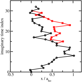
Figure 5: Illustration of the wiggle move for a single particle in a one-dimensional harmonic trap. The black circles and red squares depict the old and proposed new configurations, respectively. It is assumed that the construction of the new path segment was continued after the construction of the first midpoint bead, the next two midpoint beads, and so on.

illustrates the wiggle move for a single particle in a one-dimensional harmonic trap ($j=14$ and $s=16$). The proposed new path is constructed as follows: A new midpoint bead with index 22 is proposed and tested according to Eq. (61): If rejected (i.e., if the random number generated is smaller than ${\mathcal{A}}_{0-{\rm{th}}}$), the move is aborted in advance and the new configuration is set to the old configuration; if not rejected, the construction of the new path segment is continued (this is what is assumed in making Fig. 5). In the latter case, two new midpoint beads with index 18 and 26 are proposed and tested simultaneously according to Eq. (61). If rejected, the move is aborted in advance and the new configuration is set to the old configuration; if not rejected, four new midpoint beads with index 16, 20, 24, and 28 are proposed and tested simultaneously according to Eq. (61). If rejected, the move is aborted in advance and the new configuration is set to the old configuration; if not rejected, eight new midpoint beads with index 15, 17, 19, 21, 23, 25, and 29 are tested simultaneously according to Eq. (61). If rejected, the move is aborted with the new configuration being the old configuration; if not rejected, the move is accepted in its entirety and the path segment that involves the beads with index 15 to 29 is changed to the new position vectors.

4.3.3 Pair distance move

The pair distance move is employed in systems with two-body zero-range interactions. As discussed earlier, two-body zero-range interactions can be treated using the pair product approximation but not, to the best of our knowledge, using the Trotter formula based decomposition of the propagator. The use of the pair distance move is especially important if the two-body $s$-wave scattering length diverges. The key motivation is that two particles can, if zero-range interactions are present, be close to each other or even on top of each other. Traditional moves such as the wiggle move and the naive move, however, do not generate configurations in which particles sit on top of each other. The reason is that the scaled pair distribution function $4\pi r^{2}P_{12}(r)$ for non-interacting particles or for uniformly distributed particles is zero at $r=0$, implying that configurations with vanishing pair distance are not generated by the traditional moves. The pair distance move involves two particles with the same time slice index $j$, where $j=0,\cdots,2n$. The proposed move keeps the center of mass of the selected pair unchanged but modifies its relative distance vector.

The pair distance move can be implemented as follows. (i) Randomly choose the indices $k$, $l$ and $j$ of the single-particle beads $\mathbf{r}_{k,j}$ and $\mathbf{r}_{l,j}$ involved in the move and set $\mathbf{r}_{\rm{old}}=\mathbf{r}_{k,j}-\mathbf{r}_{l,j}$ and $r_{\rm{old}}=|\mathbf{r}_{\rm{old}}|$. Store the old center-of-mass vector $\mathbf{b}$ of the selected pair, $\mathbf{b}=(\mathbf{r}_{k,j}+\mathbf{r}_{l,j})/2$. (ii) Generate a new relative distance vector $\mathbf{r}_{\rm{new}}=\mathbf{r}_{\rm{old}}+\delta r\hat{\mathbf{r}}_{\rm{old}}$, where $\delta r$ is obtained by choosing a value uniformly from the pre-set interval $[-\Delta r,\Delta r]$. This prescription implies that $\delta r$ can be negative and that $\mathbf{r}_{\rm{new}}$, in turn, lies along the directions $\mathbf{r}_{\rm{old}}$ or $-\mathbf{r}_{\rm{old}}$. (iii) Calculate the ratio $w$, $w=(r_{\rm{old}}+\delta r)^{2}\pi_{\rm{new}}/[(r_{\rm{old}})^{2}\pi_{\rm{old}}]$. If this ratio is larger than a random number drawn uniformly from 0 to 1, accept the move and set $\mathbf{r}_{k,j}=\mathbf{b}+\mathbf{r}_{\rm{new}}/2$ and $\mathbf{r}_{l,j}=\mathbf{b}-\mathbf{r}_{\rm{new}}/2$; otherwise, reject the move (in this case, $\mathbf{r}_{k,j}$ and $\mathbf{r}_{l,j}$ remain unchanged). The value of $\Delta r$ is adjusted such that approximately 50 % of the proposed moves are accepted.

The acceptance/rejection step involves the quantity $w$. If $j$ is not equal to $0$ or $2n$, $w$ reduces to

$$w=\frac{(r_{\rm{old}}+\delta r)^{2}G(\mathbf{R}_{j-1},\mathbf{R}_{j}^{\rm{new}};\Delta\tau)G(\mathbf{R}_{j}^{\rm{new}},\mathbf{R}_{j+1};\Delta\tau)}{(r_{\rm{old}})^{2}G(\mathbf{R}_{j-1},\mathbf{R}_{j}^{\rm{old}};\Delta\tau)G(\mathbf{R}_{j}^{\rm{old}},\mathbf{R}_{j+1};\Delta\tau)}.$$ (62)

If $j$ is equal to $0$, one finds

$$w=\frac{(r_{\rm{old}}+\delta r)^{2}\psi_{T}(\mathbf{R}_{0}^{\rm{new}})G(\mathbf{R}_{0}^{\rm{new}},\mathbf{R}_{1};\Delta\tau)}{(r_{\rm{old}})^{2}\psi_{T}(\mathbf{R}_{0}^{\rm{old}})G(\mathbf{R}_{0}^{\rm{old}},\mathbf{R}_{1};\Delta\tau)}.$$ (63)

The expression for $j=2n$ is similar to that for $j=0$. In Eqs. (62)-(63), $\mathbf{R}_{j}^{\rm{new}}$ is defined as

$$\mathbf{R}_{j}^{\rm{new}}=$$

$$\{\mathbf{r}_{1},\cdots,\mathbf{r}_{k-1,j},\mathbf{b}+\mathbf{r}_{\rm{new}}/2,\mathbf{r}_{k+1,j},\cdots,\mathbf{r}_{l-1,j},\mathbf{b}-\mathbf{r}_{\rm{new}}/2,\mathbf{r}_{l+1,j},\cdots,\mathbf{r}_{N,j}\}.$$ (64)

As already alluded to, the propagator $G$ entering in the expressions for $w$ is expressed using the pair product approximation, i.e., each of the $G$’s is replaced by the expression given in Eq. (37). Careful inspection of the resulting expression for $w$ shows that a number of terms in the numerator can be canceled by corresponding terms in the denominator. However, since the reduced pair propagator $\bar{G}_{\rm{rel}}$ “connects” the $k$-th particle with all other particles and the $l$-th particle with all other particles, two products over a particle dummy index survive for each of the $G$’s, making the pair distance move computationally more expensive than the naive move implemented using the Trotter decomposition (in fact, the argument just given explains why the pair product approximation is, generally speaking, computationally more demanding than Trotter formula based schemes). The ratio $(r_{\rm{old}}+\delta r)^{2}/(r_{\rm{old}})^{2}$, which is included in the acceptance step, ensures that the small interparticle distance behavior is described properly. The reader is referred to Ref. [45] for more details.

4.4 Expectation values

The previous section outlined how to generate new configurations. Assuming that no symmetrization or anti-symmetrization is needed (see Sec. 4.6 for details) and that a suitable trial function $\psi_{T}$ is known, the missing piece for completing the PIGS algorithm is the determination of the weight function $w(\mathbf{x})$ [see Eq. (47)]. This section discusses the derivation of the form of the weight function $w(\mathbf{x})$ for selected observables; the steps outlined below can be generalized to other observables. Explicit expressions for $w(\mathbf{x})$ can be derived for many observables using either quantum estimator relations such as Eq. (12) or thermodynamic type relations such as Eq. (13). The determination of the superfluid or condensate fractions is more involved and not considered in this review.

4.4.1 Example: Energy estimator

Using the thermodynamic type relation, Eq. (13), and plugging in one of the approximate expressions for the propagator, an explicit expression for the weight function $w(\mathbf{x})$ can be derived. As an example, we consider the thermodynamic energy estimator for the second-order Trotter formula for particles without permutations. Using Eq. (19) and Eq. (25) without the ${\cal{O}}(\Delta\tau^{3})$ term in Eq. (7), the normalization factor $Z(\tau)$ reads

$$Z(\tau)=\int_{\mathbf{R}_{0}}\cdots\int_{\mathbf{R}_{2n}}\psi_{T}(\mathbf{R}_{0})\psi_{T}(\mathbf{R}_{2n})G_{0}(\mathbf{R}_{0},\mathbf{R}_{1};\Delta\tau)\times\cdots\times G_{0}(\mathbf{R}_{2n-1},\mathbf{R}_{2n};\Delta\tau)\times$$

$$\exp\left[-\Delta\tau\left(\frac{1}{2}V(\mathbf{R}_{0})+\frac{1}{2}V(\mathbf{R}_{2n})+\sum_{j=1}^{2n-1}V(\mathbf{R}_{j})\right)\right]d\mathbf{R}_{0}\cdots d\mathbf{R}_{2n}.$$ (65)

Using Eq. (65) in Eq. (13), recalling that $\tau$ is equal to $n\Delta\tau$, and denoting the energy estimator $E_{\tau}$—calculated for a finite number of time slices by $\langle E_{T}\rangle$—, we obtain

$$\braket{E_{T}}=-\frac{1}{Z(\tau)}\int_{\mathbf{R}_{0}}\cdots\int_{\mathbf{R}_{2n}}\frac{1}{2n}\psi_{T}(\mathbf{R}_{0})\psi_{T}(\mathbf{R}_{2n})\times$$

$$\frac{\partial}{\partial\Delta\tau}\Bigg{\{}G_{0}(\mathbf{R}_{0},\mathbf{R}_{1};\Delta\tau)\times\cdots\times G_{0}(\mathbf{R}_{2n-1},\mathbf{R}_{2n};\Delta\tau)\times$$

$$\exp\left[-\Delta\tau\left(\frac{1}{2}V(\mathbf{R}_{0})+\frac{1}{2}V(\mathbf{R}_{2n})+\sum_{j=1}^{2n-1}V(\mathbf{R}_{j})\right)\right]\Bigg{\}}$$

$$d\mathbf{R}_{0}\cdots d\mathbf{R}_{2n}.$$ (66)

The goal is now to rewrite the right-hand side of Eq. (66) such that we can read off $w(\mathbf{x})$ by comparing with Eq. (47). Combining Eq. (26) [without the ${\cal{O}}(\Delta\tau^{3})$ term] and Eq. (45), we recognize that Eq. (66) can be rewritten in terms of $\pi(\mathbf{x})$,

$$\braket{E_{T}}=-\frac{1}{Z(\tau)}\int_{\mathbf{x}}\frac{1}{2n}\frac{\partial\pi(\mathbf{x})}{\partial\Delta\tau}d\mathbf{x}.$$ (67)

The probability distribution $\pi(\mathbf{x})$ depends on $\Delta\tau$ through the $2n$ propagators $G_{0}$. Applying the chain rule to evaluate the derivative with respect to $\Delta\tau$, we obtain

$$\braket{E_{T}}=\frac{1}{Z(\tau)}\times$$ (68)

$$\int_{\mathbf{x}}\frac{1}{2n}\left[\sum_{j=0}^{2n-1}\left(\frac{3N}{2\Delta\tau}-\frac{(\mathbf{R}_{j}-\mathbf{R}_{j+1})^{2}}{4\lambda_{m}\Delta\tau^{2}}\right)+\frac{1}{2}V(\mathbf{R}_{0})+\frac{1}{2}V(\mathbf{R}_{2n})+\sum_{j=1}^{2n-1}V(\mathbf{R}_{j})\right]\times$$

$$\pi(\mathbf{x})d\mathbf{x}.$$

Comparing Eq. (68) with Eq. (47), one reads off

$$w(\mathbf{x})=\frac{1}{2n}\left[\sum_{j=0}^{2n-1}\left(\frac{3N}{2\Delta\tau}-\frac{(\mathbf{R}_{j}-\mathbf{R}_{j+1})^{2}}{4\lambda_{m}\Delta\tau^{2}}\right)+\frac{1}{2}V(\mathbf{R}_{0})+\frac{1}{2}V(\mathbf{R}_{2n})+\sum_{j=1}^{2n-1}V(\mathbf{R}_{j})\right].$$ (69)

The right-hand side of Eq. (69) can be evaluated straightforwardly, provided the configuration $\mathbf{x}$ is known.

Using the quantum estimator relation, Eq. (12), an alternative energy estimator can be derived. Here, we derive the quantum energy estimator for particles without permutations using the second-order Trotter formula as an example. Our goal is to rewrite Eq. (12) such that we can read off the form of $w(\mathbf{x})$ by comparing with Eq. (47). To this end, we derive an auxiliary identity [see Eq. (74)] that we use below to rewrite the integrand of the numerator of Eq. (12).

Using the position representation of the Hamiltonian $\hat{H}$ [82],

$$\braket{\mathbf{R}}{\hat{H}}{\mathbf{R}^{\prime}}=H_{\mathbf{R}}\delta(\mathbf{R}-\mathbf{R}^{\prime}),$$ (70)

where

$$H_{\mathbf{R}}=-\lambda_{m}\nabla_{\mathbf{R}}^{2}+V(\mathbf{R}),$$ (71)

one finds

$$\int_{\mathbf{R}^{\prime}}\langle\mathbf{R}|\hat{H}|\mathbf{R}^{\prime}\rangle G(\mathbf{R}^{\prime},\mathbf{R}^{\prime\prime};\tau)d\mathbf{R}^{\prime}=$$

$$\int_{\mathbf{R}^{\prime}}\left\{[-\lambda_{m}\nabla_{\mathbf{R}}^{2}+V(\mathbf{R})]\delta(\mathbf{R}-\mathbf{R}^{\prime})\right\}G(\mathbf{R}^{\prime},\mathbf{R}^{\prime\prime};\tau)d\mathbf{R}^{\prime}$$ (72)

or, integrating by parts twice,

$$\int_{\mathbf{R}^{\prime}}\langle\mathbf{R}|\hat{H}|\mathbf{R}^{\prime}\rangle G(\mathbf{R}^{\prime},\mathbf{R}^{\prime\prime};\tau)d\mathbf{R}^{\prime}=$$

$$\int_{\mathbf{R}^{\prime}}\delta(\mathbf{R}-\mathbf{R}^{\prime})\left\{[-\lambda_{m}\nabla_{\mathbf{R}}^{2}+V(\mathbf{R})]G(\mathbf{R}^{\prime},\mathbf{R}^{\prime\prime};\tau)\right\}d\mathbf{R}^{\prime}.$$ (73)

Performing the integration over $\mathbf{R}^{\prime}$ on the right-hand side of Eq. (73), we have

$$\int_{\mathbf{R}^{\prime}}\langle\mathbf{R}|\hat{H}|\mathbf{R}^{\prime}\rangle G(\mathbf{R}^{\prime},\mathbf{R}^{\prime\prime};\tau)d\mathbf{R}^{\prime}=[-\lambda_{m}\nabla_{\mathbf{R}}^{2}+V(\mathbf{R})]G(\mathbf{R},\mathbf{R}^{\prime\prime};\tau).$$ (74)

We denote the quantum estimator $E_{\tau}$ [Eq. (12)], evaluated using a finite number of time slices, by $\langle E_{H}\rangle$. Inserting the closure relation [Eq. (8)] $2n-2$ times into Eq. (12) and using Eq. (74) with $\tau$ replaced by $\Delta\tau$, we obtain

$$\braket{E_{H}}=\frac{1}{Z(\tau)}\times$$

$$\int_{\mathbf{R}_{0}}\cdots\int_{\mathbf{R}_{2n}}\psi_{T}(\mathbf{R}_{0})G(\mathbf{R}_{0},\mathbf{R}_{1};\Delta\tau)G(\mathbf{R}_{1},\mathbf{R}_{2};\Delta\tau)\times\cdots\times G(\mathbf{R}_{n-2},\mathbf{R}_{n-1};\Delta\tau)\times$$

$$\left\{[-\lambda_{m}\nabla_{\mathbf{R}_{n}}^{2}+V(\mathbf{R}_{n})]G(\mathbf{R}_{n-1},\mathbf{R}_{n};\Delta\tau)\right\}G(\mathbf{R}_{n},\mathbf{R}_{n+1};\Delta\tau)\times$$

$$G(\mathbf{R}_{n+1},\mathbf{R}_{n+2};\Delta\tau)\times\cdots\times G(\mathbf{R}_{2n-1},\mathbf{R}_{2n};\Delta\tau)\psi_{T}(\mathbf{R}_{2n})d\mathbf{R}_{0}\cdots d\mathbf{R}_{2n}.$$ (75)

Applying the second-order Trotter formula [Eq. (26) without the ${\cal{O}}(\Delta\tau^{3})$ term] to Eq. (75), we obtain

$$\braket{E_{H}}=\frac{1}{Z(\tau)}\int_{\mathbf{x}}\bigg{[}\frac{3N}{2\Delta\tau}-\frac{(\mathbf{R}_{n}-\mathbf{R}_{n-1})^{2}}{4\lambda_{m}\Delta\tau^{2}}+V(\mathbf{R}_{n})-(\mathbf{R}_{n}-\mathbf{R}_{n-1})\cdot\nabla_{\mathbf{R}_{n}}V(\mathbf{R}_{n})$$

$$+\lambda_{m}\Delta\tau\nabla_{\mathbf{R}_{n}}^{2}V(\mathbf{R}_{n})-\lambda_{m}\Delta\tau^{2}(\nabla_{\mathbf{R}_{n}}V(\mathbf{R}_{n}))^{2}\bigg{]}\pi(\mathbf{x})d\mathbf{x}.$$ (76)

Because $\hat{H}$ commutes with the propagator, $\hat{H}$ can be applied to any time slice (in the derivation above, $\hat{H}$ was applied to the $n$th time slice). This implies that one can average over all time slices to improve the accuracy (i.e., to take more “measurements” for each configuration). Averaging over all possible time slice indices, we obtain

$$\braket{E_{H}}=\frac{1}{Z(\tau)}\int_{\mathbf{x}}\frac{1}{2n}\Bigg{\{}\sum_{j=1}^{2n}\bigg{[}\frac{3N}{2\Delta\tau}-\frac{(\mathbf{R}_{j}-\mathbf{R}_{j-1})^{2}}{4\lambda_{m}\Delta\tau^{2}}+V(\mathbf{R}_{j})-(\mathbf{R}_{j}-\mathbf{R}_{j-1})\cdot\nabla_{\mathbf{R}_{j}}V(\mathbf{R}_{j})$$

$$+\lambda_{m}\Delta\tau\nabla_{\mathbf{R}_{j}}^{2}V(\mathbf{R}_{j})-\lambda_{m}\Delta\tau^{2}(\nabla_{\mathbf{R}_{j}}V(\mathbf{R}_{j}))^{2}\bigg{]}\Bigg{\}}\pi(\mathbf{x})d\mathbf{x}.$$ (77)

Comparing Eq. (77) with Eq. (47), we obtain

$$w(\mathbf{x})=\frac{1}{2n}\bigg{\{}\sum_{j=1}^{2n}\bigg{[}\frac{3N}{2\Delta\tau}-\frac{(\mathbf{R}_{j}-\mathbf{R}_{j-1})^{2}}{4\lambda_{m}\Delta\tau^{2}}+V(\mathbf{R}_{j})-(\mathbf{R}_{j}-\mathbf{R}_{j-1})\cdot\nabla_{\mathbf{R}_{j}}V(\mathbf{R}_{j})$$

$$+\lambda_{m}\Delta\tau\nabla_{\mathbf{R}_{j}}^{2}V(\mathbf{R}_{j})-\lambda_{m}\Delta\tau^{2}(\nabla_{\mathbf{R}_{j}}V(\mathbf{R}_{j}))^{2}\bigg{]}\bigg{\}}.$$ (78)

In Eq. (78), the head ($0$-th time slice) and tail ($2n$-th time slice) are not treated on equal footing because of the partial derivative. The expression can be made “symmetric” by averaging over additional terms for which the derivative yields a term that contains the factor $\mathbf{R}_{j+1}-\mathbf{R}_{j}$. Compared to Eq. (69), Eq. (78) contains three extra terms in the sum. In the $n\to\infty$ limit, both estimators approach the true expectation value. However, for finite $n$, $\langle E_{T}\rangle$ and $\langle E_{H}\rangle$ generally give different estimates of the energy. To obtain accurate results, one needs to extrapolate the finite $\Delta\tau$ calculations to the zero time step limit. The difference between the two estimators for a single $\Delta\tau$ may be used as a rough estimate of the systematic error [6].

4.4.2 Example: Structural properties

The energy estimator is special in that the information carried by all $2n+1$ time slices can be used [see the sum over $j$ in Eqs. (69) and (78)]. The reason is that the Hamiltonian operator commutes with the propagator. For other estimators, only the information carried by the middle or $n$-th time slice and the associated propagators can, in general, be used. This section exemplarily discusses the determination of structural properties within the PIGS framework.

Quite generally, the operator $\hat{D}$ corresponding to a structural observable can be written as a function $f(\mathbf{R})$ times a $\delta$-function. For example, for the scaled pair distribution function $4\pi r^{2}P_{12}(r)$ for particles one and two, $f(\mathbf{R})$ is equal to one and the $\delta$-function is equal to $\delta(r_{\rm{ref}}-|\mathbf{r}_{12}|)$, where $\mathbf{r}_{12}$ is the distance vector between particles one and two. Replacing $\langle\mathbf{R}^{\prime}|\hat{H}|\mathbf{R}^{\prime\prime\prime}\rangle$ on the right-hand side of Eq. (12) by $\delta(r_{\rm{ref}}-|\mathbf{r}_{12}|)\delta(\mathbf{R}^{\prime}-\mathbf{R}^{\prime\prime\prime})$, one finds $w(\mathbf{x})=\delta(r_{\rm{ref}}-|\mathbf{r}_{1,n}-\mathbf{r}_{2,n}|)$. Similarly to the stochastic evaluation of structural properties for a given many-body (zero-temperature) wave function, the $\delta$-function in the operator yielding the pair distribution function amounts to sorting the configurations into small intervals or bins and counting the number of configurations that fall into each of the intervals.

In practice, to obtain the scaled pair distribution function $4\pi r^{2}P_{12}(r)$ for particles one and two, we discretize the pair distance $r_{12}$, $r_{12}=|\mathbf{r}_{1}-\mathbf{r}_{2}|$, into a series of $k_{\rm{max}}$ bins $[k\delta r,(k+1)\delta r]$, where $k$ range from 0 to $k_{\rm{max}}-1$. During the simulation, the pair distance is calculated for many configurations and sorted into the bins, i.e., a histogram of the pair distances is collected. For each configuration considered (note, we may skip configurations to ensure that the samples collected have neglegible correlations), the pair distance $r_{12}$ is calculated for the middle time slice $\mathbf{R}_{n}$. The bin number $l$ of the histogram is calculated by evaluating $l={\rm{Floor}}(r_{12}/\delta r)$, where Floor$(x)$ gives the largest integer smaller or equal to $x$, and the histogram value $v_{l}$ of the $l$-th bin is increased by one. At the end, the histogram defined by the $v_{l}$ is normalized by dividing by the total number $B_{t}$ of pair distances considered and the bin size $\delta r$. The histogram created is a discretized version of the scaled pair distribution function $4\pi r^{2}P_{12}(r)$. The approach outlined yields the correct normalization even if some pair distances generated during the simulation are larger than $k_{\rm{max}}\delta r$. We typically monitor how many distances cannot be sorted into the histogram by comparing $\sum_{l}v_{l}$ with $B_{t}$. If the fraction is too large, then the “cutoff” $k_{\rm{max}}\delta r$ needs to be increased.

Because the process involved in calculating different structural properties such as the pair distribution function and triple distribution function is the same, the data structure used to accumulate different distribution functions and the accumulation process can be described by a single class in object oriented programming languages. This avoids duplication of the code. In the code, the desired estimator (the “object”) such as the pair distribution function estimator and the triple distribution function estimator can be constructed according to the same class and can be initialized with observable specific parameters such as the bin size, the bin number, and the number of particles. To accumulate the weight and finalize the results, the same virtual methods can be called for different estimators. The actual implementation of these virtual methods may or may not be the same for different estimators. For example, the scaled pair and scaled triple distribution functions can share the same implementation since both are described by an operator of the form $\delta(r_{\rm{ref}}-r)$, where $r_{\rm{ref}}$ is either the pair distance or the three-body hyperradius (see, e.g., Refs. [83, 84] for the resulting distribution function). The (unscaled) pair distribution function, in contrast, is described by an operator of the form $\delta(r_{\rm{ref}}-r)/(4\pi r^{2})$ and has to be implemented separately.

4.5 Error analysis

The expectation value $\braket{f(\mathbf{x})}$ of a function $f(\mathbf{x})$ with respect to the probability density function $p(\mathbf{x})$ is defined as

$$\braket{f(\mathbf{x})}=\int_{\mathbf{x}}f(\mathbf{x})p(\mathbf{x})d\mathbf{x}.$$ (79)

In the PIGS algorithm, we generate a finite series $X$ of configurations $\mathbf{x}_{j}$,

$$X=\{\mathbf{x}_{1},\mathbf{x}_{2},\cdots,\mathbf{x}_{M}\},$$ (80)

according to the probability distribution $\pi(\mathbf{x})$. The expectation value $\braket{{O}}$ of an operator can then be estimated by the mean value $\bar{{O}}$ of the series $X$,

$$\bar{{O}}=\frac{1}{M}\sum_{j=1}^{M}w(\mathbf{x}_{j}).$$ (81)

We refer to $\bar{{O}}$ as $\braket{{O}}_{X}$. In the limit $M\to\infty$, the mean value $\bar{{O}}$ approaches the expectation value $\braket{{O}}$ [see Eq. (47)].

According to the central limit theorem, the mean value $\bar{{O}}$ of the series $X$ approaches the expectation value $\braket{{O}}$ in a predictive manner. The “standard” central limit theorem states that the mean of a sufficiently large number of random samples, drawn from a distribution with a well-defined mean value and variance, is approximately normally distributed [59, 85]. Since the Markov chain generates a series of data that is correlated for small “lag” and uncorrelated for large “lag”, the standard central limit theorem cannot be applied directly. However, it has been shown that the central limit theorem can be extended to Markov-chain generated data [86]. Thus, we divide the series $X$, obtained from the PIGS samples $w(\mathbf{x}_{j})$, into $L$ blocks, each with $l=M/L$ configurations. Defining the block averages $S_{k}$,

$$S_{k}=\frac{1}{l}\sum_{j=(k-1)\times l+1}^{k\times l}w(\mathbf{x}_{j}),$$ (82)

we construct the series $\{S_{1},\cdots,S_{L}\}$. Provided $l$ is sufficiently large (in our applications, the value of $l$ ranges from 10 to $10^{4}$), the block averages $S_{k}$ are normally distributed and the variance $\sigma^{2}$ of the block averages can be estimated from the sample variance $\braket{\sigma^{2}}_{X}$,

$$\braket{\sigma^{2}}_{X}=\frac{1}{L-1}\sum_{j=1}^{L}(S_{j}-\bar{S}),$$ (83)

where

$$\bar{S}=\frac{1}{L}\sum_{j=1}^{L}S_{j}.$$ (84)

Note that $\bar{S}$ is equal to $\bar{{O}}$ [this can be seen by comparing Eqs. (81) and (82)]. In our simulations, we estimate the error of the expectation value $\braket{{O}}$ using $\braket{\sigma_{\bar{{O}}}}_{X}$,

$$\braket{\sigma_{\bar{{O}}}}_{X}=\sqrt{\frac{\braket{\sigma^{2}}_{X}}{L}},$$ (85)

i.e., we report the mean $\bar{{O}}$ with error $\braket{\sigma_{\bar{{O}}}}_{X}$.

In our simulations, the number $l$ of configurations per block is determined such that the block averages $S_{k}$ are normally distributed. Alternatively, the value of $l$ (and, assuming $M$ is fixed, that of $L$) can be determined by calculating the autocorrelation length [1, 77]. The latter approach is more commonly used and is somewhat simpler to implement. The two approaches should yield comparable results.

Considering $Q$ simulations, each yielding a series $X_{j}$ and correspondingly $\sqrt{\braket{\sigma^{2}}_{X_{j}}}$ (assuming finite $L$), the estimate of the standard deviation is biased because the mean value of a square root function is not equal to the square root of the mean, i.e.,

$$\frac{\sum_{j=1}^{Q}\sqrt{\braket{\sigma^{2}}_{X_{j}}}}{Q}\neq\sqrt{\frac{\sum_{j=1}^{Q}\braket{\sigma^{2}}_{X_{j}}}{Q}}.$$ (86)

Since the bias becomes negligible for sufficiently large $L$, there is no need to correct for the bias. In our simulations, $L$ is typically 80 or larger. Because the elements $S_{j}$ in $\{S_{1},\cdots,S_{L}\}$ are normally distributed, the variance $\braket{\sigma^{2}}_{X}$ is approximately a constant for sufficiently large $L$ and the error $\braket{\sigma_{\bar{{O}}}}_{X}$ scales, according to Eq. (85), as $1/\sqrt{L}$. Thus, to improve the accuracy of an observable by an order of magnitude, the computational time needs to be increased by two orders of magnitude.

To check whether the final distribution is approximately normal, one can make a histogram of the observable under study. Figure 6 shows the normalized histogram for the energy

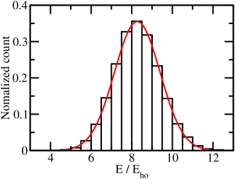
Figure 6: Normalized histogram of the energy $E/E_{\rm{ho}}$, calculated using the thermal estimator, for the harmonically trapped (3,3) system at unitarity. The histogram is constructed using 38,400 block averages generated using 480 processors (see the text for details). The red solid line shows the normal distribution with mean value of $E=8.273E_{\rm{ho}}$ and standard deviation of $1.124E_{\rm{ho}}$ (the error of the mean is $1.124E_{\rm{ho}}/\sqrt{38,400}=0.006E_{\rm{ho}}$).

of the (3,3) system at unitarity. The notation (3,3) refers to three spin-up fermions and three spin-down fermions under external harmonic confinement with angular frequency $\omega$ (the oscillator energy of $\hbar\omega$ is denoted by $E_{\rm{ho}}$). The physics of this small fermionic system is discussed in more detail in Sec. 5. The example considered here uses $\tau=0.5(E_{\rm{ho}})^{-1}$, $\Delta\tau=0.125(E_{\rm{ho}})^{-1}$, and $\psi_{T}$ given in Eq. (120); the resulting extrapolated $\Delta\tau=0$ energy is reported in Table 3. The simulation is done on $480$ processors with each processor producing 80 block averages. This yields a total of 38,400 block averages. Even though these block averages are not obtained from a single Markov chain but from 480 independent Markov chains, we calculate the mean and error of the mean using, respectively, Eqs. (84) and (85) with $L=38,400$. The resulting sample mean is $8.273E_{\rm{ho}}$ with an error or uncertainty of $0.006E_{\rm{ho}}$. Using the calculated mean and standard deviation, the solid line in Fig. 6 shows the corresponding normal distribution. It can be seen that the solid line provides a faithful description of the histogram, indicating that the underlying samples are indeed normally distributed.

The presented analysis requires a sufficiently large number of block averages. In practice, it may not be feasible or advisable to calculate many block averages. In such a case, one can check if the error scales as $\sqrt{1/L}$ with the number of blocks $L$. Reducing the number of blocks by a factor of two, one should observe that, if the block averages are normally distributed, the error increases roughly by a factor of $\sqrt{2}$. This check can be performed for as few as 5 or 10 blocks and provides, in many cases, enough information to reliably assign error bars.

To check explicitly whether the samples are independent, one needs to perform autocorrelation (or serial correlation) tests [7]. Given a series of numbers $\{x_{1},\cdots,x_{L}\}$, the lag $k$ correlation coefficient $r_{k}$, which measures the correlation of the series of numbers $\{x_{1},\cdots,x_{L-k}\}$ and $\{x_{1+k},\cdots,x_{L}\}$, is given by [87]

$$r_{k}=\frac{\sum_{j=1}^{L-k}(x_{j}-\bar{x})(x_{j+k}-\bar{x})}{\sum_{j=1}^{L}(x_{j}-\bar{x})^{2}},$$ (87)

where $\bar{x}$ denotes the average of the numbers $\{x_{1},\cdots,x_{L}\}$. If the samples are truly uncorrelated, the $r_{k}$ approximately follow a normal distribution for sufficiently large $L-k$ and the variance of $r_{k}$ is approximately equal to $1/L$. Furthermore, the probability that $r_{k}$ falls into the interval

$$\left[\frac{-1-1.96\sqrt{L-k-1}}{L-k},\frac{-1+1.96\sqrt{L-k-1}}{L-k}\right]$$ (88)

is 95% [87]. Based on hypothesis testing theory [88], it is claimed, with 95% confidence, that a sample is correlated if $r_{k}$ (based on a single test for one $k$) falls outside the interval given in Eq. (88).

Figure 7

Figure 7: The crosses show the correlation coefficient $r_{k}$ as a function of the lag $k$ ($k=1-40$) for the sample and observable considered in Fig. 6. A series of 80 block averages, obtained from a single Markov chain (and processor), is analyzed. The upper and lower solid lines show the 95% confidence interval defined in Eq. (88).

shows the correlation coefficient $r_{k}$ [Eq. (87) with $L=80$] for 80 block averages generated on a single processor (i.e., obtained from a single Markov chain) as a function of the lag $k$ for the system and observable considered in Fig. 6. Since the correlation coefficients for $k\geq 1$ all lie within the confidence band, it is said that the data pass the autocorrelation test. For the data shown in Fig. 6, similar correlation coefficient plots are obtained for each of the 80 block averages generated by the other 479 processors. This verifies that the samples are truly independent.

4.6 Permutations: On-the-fly anti-symmetrization scheme

To account for the particle statistics, one needs to ensure the proper behavior of the propagator under particle permutations. The Hilbert space for identical bosons or identical fermions is restricted compared to that of Boltzmann particles described by the same Hamiltonian. The discussion so far, including the short-time approximations for the propagator introduced in Sec. 3.1, applies to Boltzmann particles.

In the “standard” approach of generating paths for systems containing identical particles, the symmetrizer and anti-symmetrizer are evaluated stochastically (the corresponding move is referred to as “permutation move”) [6, 9]. This implies that Bose and Fermi systems are simulated by the same paths. Expectation values, in contrast, are accumulated by including “weight factors” (plus and minus signs) that account for the particle statistics. This standard approach can be thought of as an analog of a post-symmetrization scheme, where one first generates configurations that represent the entire Hilbert space and then projects out those configurations that have the proper symmetry.

Here, we introduce an alternative “on-the-fly” symmetrization/anti-symmetrization scheme that explicitly enforces the proper symmetry at each imaginary time index. This scheme is particularly useful for fermionic systems with zero-range interactions. Without a three-body regulator and without this on-the-fly anti-symmetrization scheme, two-component Fermi gases would undergo Thomas collapse [89]. A downside of the scheme discussed below is that the computational effort scales factorially with the number of identical particles; as a consequence, the scheme becomes prohibitively expensive with increasing number of particles. While the on-the-fly symmetrization scheme can be applied to systems that contain identical bosons, the explicit symmetrization is typically not needed in this case since the ground state wave function of the system in which the bosons are replaced by Boltzmann particles is identical to that of the system with bosons. Thus, the discussion in this section is most useful for fermions.

We start with a general discussion that will be useful for our on-the-fly anti-symmetrization scheme and then discuss on-the-fly anti-symmetrization scheme and PIGS specific aspects. To this end, we introduce the symmetrizer $\hat{\mathcal{P}}$ [6]. For single-component Bose and Fermi systems ($N$ identical particles), $\hat{\mathcal{P}}$ can be written as [90]

$$\hat{\mathcal{P}}=\frac{1}{N!}\sum_{\sigma}(\pm 1)^{N_{\rm{I}}(\sigma)}\hat{P}_{\sigma},$$ (89)

where $\sigma$ denotes the permutation of particle indices, $N_{\rm{I}}(\sigma)$ the number of inversions in $\sigma$ [91], and $\hat{P}_{\sigma}$ the corresponding permutation operator. The plus (minus) sign in Eq. (89) applies to identical bosons (fermions). For example, the symmetrizers (to unify the notation, we use the term symmetrizer for bosons and fermions) for two and three identical fermions are $\hat{\mathcal{P}}=\hat{\mathcal{A}}_{2}$ and $\hat{\mathcal{P}}=\hat{\mathcal{A}}_{3}$, $\hat{\mathcal{A}}_{2}=(1-\hat{P}_{12})/2$ and $\hat{\mathcal{A}}_{3}=(1-\hat{P}_{12}-\hat{P}_{13}-\hat{P}_{23}+\hat{P}_{123}+\hat{P}_{132})/6$, respectively. Here, $\hat{P}_{ijk\cdots l}$ replaces the identity of particle $i$ (i.e., its entire “information” including spatial coordinates, spin degrees of freedom, etc.) with that of particle $j$, that of particle $j$ with that of particle $k$, $\cdots$, and that of particle $l$ with that of particle $i$. The symmetrizer $\hat{\mathcal{P}}$ commutes with $\hat{P}_{ij}$ if the $i$-th and $j$-th particles are identical. In the previous examples, $\hat{\mathcal{A}}_{2}$ commutes with $\hat{P}_{12}$ and $\hat{\mathcal{A}}_{3}$ commutes with $\hat{P}_{12}$, $\hat{P}_{13}$, and $\hat{P}_{23}$. The definition of the symmetrizer $\hat{\mathcal{P}}$ can be generalized to multi-component Bose and Fermi systems as well as Bose-Fermi mixtures. In these cases, the total symmetrizer is written as a product of symmetrizers for each component. For example, the symmetrizer for the mixture of two identical bosons (particles 1 and 2) and two identical fermions (particles 3 and 4) reads $(1+\hat{P}_{12})(1-\hat{P}_{34})/4$.

The symmetrizer $\hat{\mathcal{P}}$ also commutes with the Hamiltonian $\hat{H}$ and the propagator $\hat{G}$. $\hat{\mathcal{P}}$ serves the purpose of projecting out the wave functions that satisfy the proper exchange symmetry, i.e., it divides the Hilbert space into two parts: (i) If $\psi_{s}$ is an eigen state with the proper symmetry, then one has $\hat{\mathcal{P}}\psi_{s}=\psi_{s}$. (ii) If, in contrast, $\psi_{\rm{ns}}$ is an eigen state that does not have the proper exchange symmetry, then we have $\hat{\mathcal{P}}\psi_{\rm{ns}}=0$. We note that the eigen values of the symmetrizer $\hat{\mathcal{P}}$ are 0 and 1 while those of the two-particle permute operator $\hat{P}_{12}$ are $-1$ and 1. As we will show in the following, the fact that the eigen values of $\hat{\mathcal{P}}$ are either 0 or 1 implies

$$\hat{\mathcal{P}}^{2}=\hat{\mathcal{P}}.$$ (90)

To prove Eq. (90), we introduce a unitary matrix $\mathcal{U}$ that diagonalizes the Hermitian symmetrizer $\hat{\mathcal{P}}$, i.e., $\mathcal{U}$ is constructed such that $\hat{\mathcal{D}}=\mathcal{U}\hat{\mathcal{P}}\mathcal{U}^{-1}$ is diagonal. Because $\hat{\mathcal{P}}$ and $\hat{\mathcal{D}}$ are related through a unitary transformation, $\hat{\mathcal{D}}$ and $\hat{\mathcal{P}}$ share the same eigen values. Since the eigen values of $\hat{\mathcal{D}}$ are either 0 or 1, $\hat{\mathcal{D}}$ is diagonal with diagonal elements 0 or 1. This implies that $\hat{\mathcal{D}}^{2}$ is equal to $\hat{\mathcal{D}}$. We now rewrite $\hat{\mathcal{P}}^{2}$ using $\hat{\mathcal{P}}=\mathcal{U}^{-1}\hat{\mathcal{D}}\mathcal{U}$,

$$\hat{\mathcal{P}}^{2}=(\mathcal{U}^{-1}\hat{\mathcal{D}}\mathcal{U})(\mathcal{U}^{-1}\hat{\mathcal{D}}\mathcal{U}).$$ (91)

Using $\mathcal{U}^{-1}\mathcal{U}=1$, we have

$$\hat{\mathcal{P}}^{2}=\mathcal{U}^{-1}\hat{\mathcal{D}}\hat{\mathcal{D}}\mathcal{U}.$$ (92)

Since $\hat{\mathcal{D}}^{2}$ is equal to $\hat{\mathcal{D}}$ (see above), one finds $\hat{{\mathcal{P}}}^{2}={\mathcal{U}}^{-1}\hat{\mathcal{D}}{\mathcal{U}}$ and thus ${\hat{\mathcal{P}}}^{2}=\hat{\mathcal{P}}$, which is what we set out to prove.

The symmetrized propagator can, as we prove below, be written as $\hat{G}_{\rm{unsymm}}\hat{\mathcal{P}}$, where $\hat{G}_{\rm{unsymm}}$ is the unsymmetrized propagator, i.e., the propagator for the corresponding system with Boltzmann particles. In position space, the symmetrized propagator $G(\mathbf{R},\mathbf{R}^{\prime},\hat{\mathcal{P}};\tau)$ can be rewritten as [6]

$$G(\mathbf{R},\mathbf{R}^{\prime},\hat{\mathcal{P}};\tau)=\braket{\mathbf{R}}{\exp(-\tau\hat{H})\hat{\mathcal{P}}}{\mathbf{R}^{\prime}}$$ (93)

or as a sum over the unsymmetrized propagators,

$$G(\mathbf{R},\mathbf{R}^{\prime},\hat{\mathcal{P}};\tau)\propto\sum_{\sigma}{\rm{sgn}}(\sigma)G(\mathbf{R},\hat{\mathcal{P}}_{\sigma}\mathbf{R}^{\prime};\tau),$$ (94)

where ${\rm{sgn}}(\sigma)$ is the sign for the permutation $\sigma$ (for single-component fermions, ${\rm{sgn}}(\sigma)=(-1)^{N_{\rm{I}}(\sigma)}$). In Eq. (94), we use the proportionality symbol since the “normalization factor” depends on the number of identical particles in the system (for $N$ identical particles, the proportionality symbol becomes an equal sign if the right-hand-side is multiplied by $(N!)^{-1}$).

We now prove that $\hat{G}_{\rm{unsymm}}\hat{\mathcal{P}}$ is, indeed, the symmetrized propagator. In Schrödinger quantum mechanics, the symmetrized propagator in position space reads

$$G(\mathbf{R},\mathbf{R}^{\prime},\hat{\mathcal{P}};\tau)=\braket{\mathbf{R}}{\exp(-\tau\hat{H})\sum_{j}\ket{\psi_{{\rm{symm}},j}}\bra{\psi_{{\rm{symm}},j}}\mathbf{R}^{\prime}},$$ (95)

where $\{\psi_{{\rm{symm}},j}\}$ is the complete set of symmetrized eigen states, e.g., for $N$ identical bosons or $N$ identical fermions. The complete set of unsymmetrized eigen states of $\hat{H}$, i.e., the set of eigen states for Boltzmann particles is denoted by $\{\psi_{{\rm{unsymm}},j}\}$. Recall that the $\hat{\mathcal{P}}$ operator can be diagonalized using the unitary matrix $\mathcal{U}$. $\mathcal{U}$ “reorganizes” the eigen states $\psi_{{\rm{unsymm}},j}$ such that the new eigen states are also eigen states of $\hat{\mathcal{P}}$. The resulting eigen states $\psi_{r,j}$,

$$\psi_{r,j}=\sum_{l}\mathcal{U}_{jl}\psi_{{\rm{unsymm}},l},$$ (96)

either have the proper symmetry, i.e., $\hat{\mathcal{P}}\psi_{r,j}$ is equal to $\psi_{r,j}$ (in this case, the eigen value of $\hat{\mathcal{P}}$ is 1) or $\hat{\mathcal{P}}\psi_{r,j}$ gives zero (in this case, the eigen value of $\hat{\mathcal{P}}$ is 0). The subset of eigen states $\{\psi_{r,j}\}$, for which $\hat{\mathcal{P}}\psi_{r,j}$ is equal to $\psi_{r,j}$, coincides with the complete set of symmetrized eigen states. This process of constructing a set of properly symmetrized eigen states from a complete set of unsymmetrized eigen states is known as post-symmetrization. For later reference, we write down the auxiliary identity

$$\mathcal{U}\sum_{l}\ket{\psi_{{\rm{unsymm}},l}}\bra{\psi_{{\rm{unsymm}},l}}\mathcal{U}^{-1}=\sum_{l}\ket{\psi_{r,l}}\bra{\psi_{r,l}},$$ (97)

which can be obtained using the matrix form of Eq. (96),

$$\{\psi_{r,1},\psi_{r,2},\dots\}^{T}=\mathcal{U}\{\psi_{{\rm{unsymm}},1},\psi_{{\rm{unsymm}},2},\dots\}^{T}.$$ (98)

We now manipulate the right-hand side of Eq. (93) so that it can be readily related to Eq. (95). Starting with the right-hand side of Eq. (93) and using Eq. (90), we find

$$\braket{\mathbf{R}}{\exp(-\tau\hat{H})\hat{\mathcal{P}}}{\mathbf{R}^{\prime}} =\braket{\mathbf{R}}{\exp(-\tau\hat{H})\hat{\mathcal{P}}\hat{\mathcal{P}}}{\mathbf{R}^{\prime}}.$$ (99)

Inserting $\mathcal{U}\mathcal{U}^{-1}=\hat{1}$ and then

$$\sum_{l}\ket{\psi_{{\rm{unsymm}},l}}\bra{\psi_{{\rm{unsymm}},l}}=\hat{1},$$ (100)

we find

$$\braket{\mathbf{R}}{\exp(-\tau\hat{H})\hat{\mathcal{P}}}{\mathbf{R}^{\prime}} =\braket{\mathbf{R}}{\exp(-\tau\hat{H})\hat{\mathcal{P}}\mathcal{U}\sum_{l}\ket{\psi_{{\rm{unsymm}},l}}\bra{\psi_{{\rm{unsymm}},l}}\mathcal{U}^{-1}\hat{\mathcal{P}}}{\mathbf{R}^{\prime}}.$$ (101)

Using Eq. (97) in Eq. (101), we find

$$\braket{\mathbf{R}}{\exp(-\tau\hat{H})\hat{\mathcal{P}}}{\mathbf{R}^{\prime}} =\braket{\mathbf{R}}{\exp(-\tau\hat{H})\hat{\mathcal{P}}\sum_{l}\ket{\psi_{r,l}}\bra{\psi_{r,l}}\hat{\mathcal{P}}}{\mathbf{R}^{\prime}}.$$ (102)

Finally, noting that $\hat{\mathcal{P}}\sum_{l}\ket{\psi_{r,l}}\bra{\psi_{r,l}}\hat{\mathcal{P}}$ is equal to $\sum_{l}\ket{\psi_{{\rm{symm}},l}}\bra{\psi_{{\rm{symm}},l}}$, we arrive at

$$\braket{\mathbf{R}}{\exp(-\tau\hat{H})\hat{\mathcal{P}}}{\mathbf{R}^{\prime}} =\braket{\mathbf{R}}{\exp(-\tau\hat{H})\sum_{l}\ket{\psi_{{\rm{symm}},l}}\bra{\psi_{{\rm{symm}},l}}\mathbf{R}^{\prime}},$$ (103)

i.e., we have proven that $\hat{G}_{{\rm{unsymm}}}\hat{\mathcal{P}}$ [the left-hand side of Eq. (103) in position space] is identical to the symmetrized propagator in position space in Schrödinger quantum mechanics [Eq. (95)].

Replacing the propagator $\braket{\mathbf{R}}{\exp(-\tau\hat{H})}{\mathbf{R}^{\prime}}$ by $\braket{\mathbf{R}}{\exp(-\tau\hat{H})\hat{\mathcal{P}}}{\mathbf{R}^{\prime}}$ in all expressions involving the propagator (such as the normalization factor $Z(\tau)$, the probability distribution $\pi(\mathbf{x})$, and the weight function $w(\mathbf{x})$), we have all elements of the PIGS algorithm for bosons and fermions; as indicated at the beginning of this section, the trial function $\psi_{T}$ will be discussed in Sec. 5 for specific examples. The symmetrized probability distribution $\pi_{{\rm{symm}}}(\mathbf{x})$, e.g., reads

$$\pi_{{\rm{symm}}}(\mathbf{R}_{0},\cdots,\mathbf{R}_{2n})=\psi_{T}(\mathbf{R}_{0})G(\mathbf{R}_{0},\mathbf{R}_{1},\hat{\mathcal{P}};\Delta\tau)G(\mathbf{R}_{1},\mathbf{R}_{2},\hat{\mathcal{P}};\Delta\tau)$$

$$\times\cdots\times G(\mathbf{R}_{2n-1},\mathbf{R}_{2n},\hat{\mathcal{P}};\Delta\tau)\psi_{T}(\mathbf{R}_{2n}),$$ (104)

where each symmetrized propagator is a sum over unsymmetrized propagators with permuted configurations. This implies that the complexity of the symmetrized PIGS algorithm is increased by up to a factor of $N!$ compared to the non-symmetrized PIGS algorithm.

Since the symmetrizer is applied at each link [see Eq. (104)], the number of operations needed to evaluate the symmetrized propagator scales as $2nN!$ for $N$ identical particles. This implies that the on-the-fly symmetrization scheme becomes inefficient if the number of time slices is too large; Sec. 5 demonstrates that reliable results for two-component Fermi gases can be obtained for a series of $n$ as small as $1$, $2$ and $4$. If the Trotter formula is used, some terms can typically be pulled out of the sum over the permutations, reducing the computational effort somewhat. If the pair product approximation is used, analogous simplifications are, in general, not possible. However, as mentioned at the beginning of this section, the on-the-fly symmetrization scheme is particularly useful for fermionic systems with zero-range interactions, which cannot be treated using the Trotter formula.

The change of the probability distribution from $\pi(\mathbf{x})$ to $\pi_{\rm{symm}}(\mathbf{x})$ needs to be accounted for in the implementation of the moves and the collection of the expectation values. For example, the acceptance function for the naive move is equal to $\pi_{\rm{symm}}(\mathbf{x})$, implying that ${\cal{A}}(\mathbf{x}\rightarrow\mathbf{x}^{\prime})$ in Eq. (53) is given by $\min(1,\pi_{\rm{symm}}(\mathbf{x}^{\prime})/\pi_{\rm{symm}}(\mathbf{x}))$. The pair distance move has to be modified analogously. To obtain the acceptance function for the wiggle move, the derivation outlined in Sec. 4.3.2 needs to be carried out using the symmetrized propagator. Similarly, the estimators need to be changed accordingly. For example, to account for the permutations in the thermodynamic energy estimator $\langle E_{T}\rangle$, $\pi(\mathbf{x})$ and $Z(\tau)$ in Eq. (66) have to be replaced by the corresponding symmetrized quantities. If we wrote out, in analogy to Eq. (69), the fully symmetrized expression for the weight function $w(\mathbf{x})$ using the second-order Trotter formula, it would be rather lengthy since the symmetrized propagator contains a sum over permutations at each time slice.

The ground state of fermionic systems usually corresponds to an excited state of the corresponding system with Boltzmann statistics. This implies that explicit anti-symmetrization is necessary to propagate the trial function to the ground state with the correct particle statistics. The anti-symmetrization introduces a “sign problem” since the probability distribution can be positive or negative. The fact that the probability distribution can take either sign can be dealt with using the ideas of Refs. [83, 92].

The probability distribution for a given configuration can take either sign. Integrating all the positive (negative) portions, we obtain $Z_{+}$ ($Z_{-}$). The normalization factor $Z(\tau)$ is the sum of $Z_{+}$ and $Z_{-}$, $Z(\tau)=|Z_{+}|-|Z_{-}|$. When accumulating observables, the sign needs to be kept track of. In general, the expectation value of an observable $O$ can be written as

$$\braket{{O}}=\frac{|Z_{+}|}{|Z_{+}|-|Z_{-}|}\braket{{O}_{+}}-\frac{|Z_{-}|}{|Z_{+}|-|Z_{-}|}\braket{{O}_{-}}.$$ (105)

For the thermal energy estimator, e.g., this can be worked out explicitly. Using $Z(\tau)=|Z_{+}|-|Z_{-}|$, we find

$$\braket{{E_{T}}}=-(|Z_{+}|-|Z_{-}|)^{-1}\frac{\partial(|Z_{+}|-|Z_{-}|)}{\partial\tau}$$ (106)

or

$$\braket{{E_{T}}}=(|Z_{+}|-|Z_{-}|)^{-1}\left(|Z_{+}|\braket{{E_{T,+}}}-|Z_{-}|\braket{{E_{T,-}}}\right),$$ (107)

where

$$\braket{{E_{T,\pm}}}=-(|Z_{\pm}|)^{-1}\frac{\partial(|Z_{\pm}|)}{\partial\tau}.$$ (108)

In an actual calculation, the contributions $\langle O_{+}\rangle$ and $\langle O_{-}\rangle$ to the estimator are first calculated separately and then weighted according to their relative magnitudes. Alternatively, Eq. (105) can be written as

$$\braket{{O}}=S^{-1}\left(\frac{|Z_{+}|}{|Z_{+}|+|Z_{-}|}\braket{{O}_{+}}+\frac{|Z_{-}|}{|Z_{+}|+|Z_{-}|}\braket{{-O}_{-}}\right),$$ (109)

where

$$S=\frac{|Z_{+}|-|Z_{-}|}{|Z_{+}|+|Z_{-}|}.$$ (110)

This suggests that one can think of the simulation as yielding a purely positive normalization factor $|Z_{+}|+|Z_{-}|$; however, if one does so, a minus sign needs to be included in the observable if the probability distribution for the chosen configuration is negative. The final result is obtained if the expression is multiplied by the factor $S$.

In Eqs. (105) and (109), the term $|Z_{+}|-|Z_{-}|$ appears in the denominator. If $|Z_{+}|$ becomes closer to $|Z_{-}|$ with increasing propagation time, then the simulation becomes increasingly more challenging since the statistical noise needs to be smaller than the difference between $|Z_{+}|$ and $|Z_{-}|$.

Finally, one may wonder if there are any constraints on the trial function $\psi_{T}$. For the fixed-node diffusion Monte Carlo simulations, the trial function $\psi_{T}$ needs to be an eigen state of the symmetrizer. This is not the case for PIGS simulations because the symmetrized propagator projects out the corresponding wave function.

5 Application to fermionic systems

5.1 General considerations

This section discusses applications of the PIGS algorithm to harmonically-trapped equal-mass two-component Fermi gases consisting of $n_{1}$ spin-up and $n_{2}$ spin-down particles ($N=n_{1}+n_{2}$) in three-dimensional space. We refer to these systems as $(n_{1},n_{2})$. The model Hamiltonian $\hat{H}$ reads

$$\hat{H}=\hat{H}_{\rm{free-space}}+\hat{V}_{\rm{trap}},$$ (111)

where

$$\hat{H}_{\rm{free-space}}=\sum_{j=1}^{N}\frac{-\hbar^{2}}{2m}\nabla_{j}^{2}+\sum_{j=1}^{N-1}\sum_{k>j}^{N}V_{\rm{F}}(r_{jk}).$$ (112)

The interspecies two-body zero-range potential $V_{\rm{F}}(r_{jk})$ is given in Eq. (40) and the confining potential $\hat{V}_{\rm{trap}}$ with angular trapping frequency $\omega$ reads

$$\hat{V}_{\rm{trap}}=\frac{1}{2}m\omega^{2}\sum_{j=1}^{N}\mathbf{r}_{j}^{2}.$$ (113)

Throughout this section, we assume that the interspecies two-body interaction is characterized by an infinitely large $s$-wave scattering length $a_{s}$, i.e., we consider systems at unitarity. Like fermions are assumed to be non-interacting, i.e., no intraspecies interactions are considered. This assumption is realized in cold atom systems provided one operates at magnetic field strengths away from $p$- and higher-partial-wave resonances. As discussed in Secs. 3.3-3.5, two-body zero-range interactions are most conveniently treated using the pair product approximation. In the calculations presented below, the reduced relative propagator $\bar{G}^{\rm{rel}}(\mathbf{r},\mathbf{r}^{\prime};\tau)$ [Eq. (43)], which accounts for the two-body zero-range interactions, the kinetic energy, and the relative two-body confining potential, is being used.

The Hamiltonian $\hat{H}$ is, for infinitely large $a_{s}$, characterized by one (meaningful) length scale, the harmonic oscillator length $a_{\rm{ho}}$, $a_{\rm{ho}}=\sqrt{\hbar/(m\omega)}$. The harmonic oscillator length also characterizes the non-interacting system. The range of the interaction potential, which is zero, and the $s$-wave scattering length, which is infinitely large, do not define meaningful length scales. Moreover, for two-component fermions with equal masses, the three-body system in free space is unbound, implying that the three-body system does not introduce a new (finite) length scale; in particular, Efimov physics is absent [93, 94]. In what follows, we express lengths in units of $a_{\rm{ho}}$ and energies in units of the harmonic oscillator energy $E_{\rm{ho}}$, $E_{\rm{ho}}=\hbar\omega$.

Two-component Fermi gases with vanishing interaction range and infinitely large interspecies $s$-wave scattering length have been and continue to be a paradigmatic strongly-correlated system, for which few analytical results are known and which are challenging to treat numerically. The PIGS applications presented in this section have not been published before. The examples are chosen for their pedagogical value and for their relevance with regards to obtaining a more complete understanding of small two-component Fermi gases. Two types of systems are considered, spin-balanced systems ($n_{1}=n_{2}=N/2$; see Sec. 5.2) and spin-imbalanced systems ($n_{1}=N-1$ and $n_{2}=1$; see Sec. 5.3).

5.2 Spin-balanced Fermi gas

The ground state of spin-balanced two-component Fermi gases has $(L,\Pi)=(0,+1)$ symmetry, i.e., vanishing total orbital angular momentum $L$ and positive parity $\Pi$. Intuitively, this can be understood by realizing that each spin-up fermion is paired with a spin-down fermion. In reality, the pairing respects the identical particle characteristics, i.e., each spin-up fermion is paired with $(1/n_{2})$-th of each spin-down fermion and each spin-down fermion is paired with $(1/n_{1})$-th of each spin-up fermion. The particle statistics is enforced along the paths by explicitly applying the symmetrizer to each of the $2n$ propagators [see, e.g., Eq. (104) for the symmetrized probability distribution]. The applications below use trial functions $\psi_{T}$ that have the proper particle symmetry build in. In general, one could employ any trial function that has finite overlap with the eigen state to be determined. In practice, however, it seems best to build as much “prior knowledge” as possible into the trial function.

In the following, we discuss the construction of the trial function $\psi_{T}(\mathbf{R})$ and the dependence of the energy on the variational parameters entering into $\psi_{T}$. In addition, the convergence of the energy with respect to the total imaginary propagation time $\tau$ is analyzed. As can be seen from Eq. (3) and the surrounding discussion, $\tau$ should, in principle, be taken to infinity to allow for the excited state contributions to fully die out. In practice, this is not feasable since the noise or error that arises due to the anti-symmetrization (the sign error) increases with increasing $\tau$. Thus, the task is to find a regime of $\tau$ values, for which the excited state contributions can be neglected and the sign error is sufficiently small. For each fixed $\tau$ simulation, the convergence of the results with respect to $\Delta\tau$ or, equivalently, the number of time slices needs to be checked. Typically, for each fixed $\tau$, the results for several $n$ are, in a first step, extrapolated to the infinite $n$ limit. In a second step, the $n\rightarrow\infty$ results for several $\tau$ are considered to determine for which $\tau$ excited state contributions can be neglected. In considering larger $\tau$, it has to be checked that the sign error is sufficiently small. Last, the calculations should, ideally, be repeated for different $\psi_{T}$ to ensure that the trial function does not introduce a bias. Having an overview of the general PIGS procedure, we now discuss the construction of the trial function $\psi_{T}$.

Quite generally, the construction of the trial function is guided by physical considerations. For example, one may parameterize the trial function $\psi_{T}$ in terms of a set of variational parameters $\boldsymbol{\alpha}$, which are optimized by minimizing the expectation value of the Hamiltonian, calculated using $\psi_{T}$, with respect to the variational parameters $\boldsymbol{\alpha}$. A good trial function $\psi_{T}$ is associated with a small energy variance. In fact, if the variance is zero, the trial function coincides with one of the exact eigen states of the model Hamiltonian. While the outlined optimization strategy has been applied quite fruitfully to a number of systems, it cannot—in general—be used for the model Hamiltonian and trial functions considered in this article since both the kinetic energy and the potential energy expectation values diverge for Hamiltonian with zero-range interactions. For an exact eigen state, the divergencies cancel, yielding a finite energy expectation value. For a trial function that does not fulfill the boundary conditions imposed by the two-body zero-range interactions (see below), the infinities prevent one from estimating the energy expectation value reliably. As a consequence, we optimize the “variational parameters” contained in $\psi_{T}$ using the PIGS approach itself or using analytical arguments.

To motivate the functional form of our trial function $\psi_{T}$, we consider the behavior of the many-body eigen function $\psi$ when a spin-up fermion (particle $j$) and a spin-down fermion (particle $k$) approach each other while the other $3N-3$ coordinates, collectively denoted by $\mathbf{Y}$, where $\mathbf{Y}=\{(\mathbf{r}_{j}+\mathbf{r}_{k})/2,\mathbf{r}_{1},\cdots,\mathbf{r}_{j-1},\mathbf{r}_{j+1},\cdots,\mathbf{r}_{k-1},\mathbf{r}_{k+1},\cdots,\mathbf{r}_{N}\}$, are kept fixed [37],

$$\psi|_{r_{jk}\to 0}\propto\left(\frac{1}{r_{jk}}-\frac{1}{a_{s}}\right)B(\mathbf{Y}).$$ (114)

Here, $B$ is a function that is independent of the distance vector $\mathbf{r}_{jk}$. The Bethe-Peierls boundary condition, Eq. (114), is a direct consequence of the interspecies two-body zero-range interactions and holds for any up-down pair distance $r_{jk}$. If the scattering length $a_{s}$ diverges, as assumed throughout this section, the boundary condition reduces to

$$\psi|_{r_{jk}\to 0}\propto\frac{1}{r_{jk}}B(\mathbf{Y}).$$ (115)

The trial function is constructed such that $\psi_{T}$ (i) approximately fulfills the boundary condition, Eq. (115); (ii) approximately describes a state containing $N/2$ up-down pairs; (iii) changes sign under the exchange of any two identical fermions; (iv) approximately accounts for the external harmonic confinement; and (v) has $(L,\Pi)=(0,+1)$ symmetry.

Guideline (ii) suggests a term of the form $\prod_{j=1}^{N/2}(r_{j,N/2+j})^{-1}$. This term fulfills the boundary condition for the pairs containing the first and $(N/2+1)$-st particle, the second and $(N/2+2)$-nd particle, and so on but not the boundary condition for pairs containing, e.g., the first and $(N/2+2)$-nd particle. Application of the symmetrizer $\hat{\mathcal{P}}$ makes the short-distance behavior “less ideal”. To see this, let us exemplarily consider the $(n_{1},n_{2})=(2,2)$ system and act with $\hat{\mathcal{P}}$ onto $(r_{13}r_{24})^{-1}$,

$$\hat{\mathcal{P}}\left(\frac{1}{r_{13}r_{24}}\right)=\frac{1}{2r_{13}r_{24}}-\frac{1}{2r_{23}r_{14}}.$$ (116)

Rewriting the second term on the right-hand side of Eq. (116) in terms of the independent Jacobi vectors $\mathbf{r}_{13}$, $\mathbf{r}_{24}$, and $\mathbf{r}_{13,24}$, where $\mathbf{r}_{13,24}=\mathbf{r}_{2}+\mathbf{r}_{4}-(\mathbf{r}_{1}+\mathbf{r}_{3})$ (these coordinates correspond to one of the so-called H-trees [95]), we obtain

$$\hat{\mathcal{P}}\left(\frac{1}{r_{13}r_{24}}\right)=\frac{1}{2r_{13}r_{24}}-\frac{2}{|\mathbf{r}_{13,24}+\mathbf{r}_{13}-\mathbf{r}_{24}||\mathbf{r}_{13,24}-\mathbf{r}_{13}+\mathbf{r}_{24}|}.$$ (117)

It can now be seen that the right-hand side of Eq. (117) cannot be brought into the form of Eq. (115), implying that application of the symmetrizer leads to a functional form for which neither the “paired” nor the “unpaired” interspecies distances obey the Bethe-Peierls boundary condition.

Attempting to find a compromise between guidelines (i) and (ii), we write $\psi_{T}(\mathbf{R})$ as

$$\psi_{T}(\mathbf{R})=f_{\rm{trap}}(\mathbf{R})\Phi_{\alpha}(\mathbf{R}),$$ (118)

where $f_{\rm{trap}}(\mathbf{R})$ accounts for the external confinement,

$$f_{\rm{trap}}(\mathbf{R})=\exp\left(-\sum_{j=1}^{N}\frac{\mathbf{r}_{j}^{2}}{2a_{\rm{ho}}^{2}}\right),$$ (119)

and $\Phi_{\alpha}(\mathbf{R})$ for the correlations,

$$\Phi_{\alpha}(\mathbf{R})=(a_{\rm{ho}})^{-\alpha N/2(N/2-1)-N}\hat{\mathcal{P}}\left(\frac{\prod_{j=1}^{N/2}\prod_{k=1,k\neq j}^{N/2}\left(r_{j,N/2+k}\right)^{\alpha}}{\prod_{j=1}^{N/2}r_{j,N/2+j}}\right).$$ (120)

It can be readily checked that the right hand side of Eq. (120) has units of $length^{-3N/2}$, as required for a $3N$-particle wave function. Since $\Phi_{\alpha}(\mathbf{R})$ depends only on scalars, i.e., interparticle distances, $\psi_{T}(\mathbf{R})$ has the desired $(L,\Pi)=(0,+1)$ symmetry. In Eq. (118), $\alpha$ is an adjustable parameter. For $\alpha=0$, $\Phi_{\alpha}(\mathbf{R})$ fulfills the Bethe-Peierls boundary condition for all up-down pairs, provided the symmetrizer $\hat{\mathcal{P}}$ is dropped. A finite value of $\alpha$ reduces the probability of spin up-spin down particles that are “not paired” via the product in the denominator to be close to each other. We pursue two avenues to determine the optimal $\alpha$. We use results from the literature to fix $\alpha$, and we determine the optimal $\alpha$ by analyzing our PIGS results.

To determine $\alpha$ using literature results, we rewrite the time-independent Schrödinger equation in terms of the hyperspherical coordinates $R$ and $\mathbf{\Omega}$, where $R$ denotes the hyperradius,

$$R^{2}=\sum_{k=1}^{N}\mathbf{r}_{k}^{2},$$ (121)

and $\mathbf{\Omega}$ the $3N-1$ hyperangles. Note that the hyperradius $R$, which is simply given by $|\mathbf{R}|$, is defined without separating off the center-of-mass degrees of freedom. For our purposes, the exact definition of the hyperangles is not important. The key ingredient for our train of thought is that the hyperradial and hyperangular degrees of freedom decouple when the $s$-wave scattering length is infinitely large [96]. The eigen value of the hyperangular equation [we denote the hyperangular function by $\phi_{\nu}(\mathbf{\Omega})$] is typically written in terms of $s_{\nu}$, which—in turn—determines the total energy of the system, $E_{\nu q}=(2q+s_{\nu}+1)E_{\rm{ho}}$, where $E_{\nu q}$ includes the center-of-mass energy of $3E_{\rm{ho}}/2$, $5E_{\rm{ho}}/2,\cdots$, and $q$ is the hyperradial quantum number, which takes the values $q=0,1,\cdots$. Writing the total wave function $\psi$ as $R^{-(3N-1)/2}F_{\nu q}(R)\phi_{\nu}(\mathbf{\Omega})$, the hyperradial Schrödinger-like equation reads

$$\left[-\frac{\hbar^{2}}{2m}\frac{\partial^{2}}{\partial R^{2}}+V_{\rm{eff}}(R)+\frac{1}{2}m\omega R^{2}\right]F_{\nu q}(R)=E_{\nu q}F_{\nu q}(R),$$ (122)

where

$$V_{\rm{eff}}(R)=\frac{\hbar^{2}(s_{\nu}^{2}-1/4)}{2mR^{2}}.$$ (123)

Solving the differential equation, one finds

$$F_{\nu q}(R)=\exp\left(-\frac{R^{2}}{2(a_{\rm{ho}})^{2}}\right)\frac{R^{s_{\nu}+1/2}}{(a_{\rm{ho}})^{s_{\nu}+1}}L_{q}^{(s_{\nu})}\left((R^{2}/(a_{\rm{ho}})^{2}\right),$$ (124)

where $L_{q}^{(s_{\nu})}$ denotes the associated Laguerre polynomial and $F_{\nu q}(R)$ is normalized according to $\int_{0}^{\infty}|F_{\nu q}(R)|^{2}dR=1$. For the ground state ($q=0$, $\nu=0$, and no center-of-mass excitations), the hyperradial solution becomes

$$F_{00}(R)=\exp\left(-\frac{R^{2}}{2(a_{\rm{ho}})^{2}}\right)\frac{R^{s_{0}+1/2}}{(a_{\rm{ho}})^{s_{0}+1}}.$$ (125)

Comparing the power of $a_{\rm{ho}}$ on the right-hand side of Eq. (120) with the power of $a_{\rm{ho}}$ in Eq. (125), we deduce

$$\alpha N/2(N/2-1)+N=s_{0}+1$$ (126)

or

$$\alpha=\frac{E_{00}/E_{\rm{ho}}-N}{N/2(N/2-1)}.$$ (127)

Using this reasoning, $\alpha$ can be estimated using the ground state energy of the $(N/2,N/2)$ Fermi system. Selected $\alpha$ values, obtained using the energies reported in Ref. [97], are shown in column 2 of Table 3. Our first set of PIGS calculations use the value of $\alpha$ reported in Table 3. In a second set of calculations, $\alpha$ is varied and optimized using the PIGS results themselves. We emphasize that the trial function constructed above provides a fairly descent description of the hyperradial degree of freedom. The hyperangular degrees of freedom are, however, less well described; we return to this point below.

Table 3: Spin-balanced two-component Fermi gas ($N/2\leq 5$) with zero-range interactions at unitarity. Column 1 lists the $(N/2,N/2)$ system considered. Column 2 reports the value of $\alpha$, obtained from Eq. (127) using the energies reported in Ref. [97]. Columns 3-6 show the propagation time $\tau$, the scheme used to extrapolate the energy to $\Delta\tau=0$, the $n$ used (the number of time slices is $2n+1$), and the resulting extrapolated $\Delta\tau=0$ PIGS energy $E_{\rm{PIGS}}$ with error bars, respectively. The abbreviation “extrap.” in the header of column 4 stands for “extrapolation” and “4-th” and “2-nd” are to be read as “4-th order” and “2-nd order”, respectively. For comparison, columns 7 and 8 show energies from the literature, obtained using the explicitly correlated Gaussian (ECG) approach [97] (the energies are denoted by $E_{\rm{ECG}}$) and the diffusion Monte Carlo method [98] (the energies are denoted by $E_{\rm{DMC}}$), respectively; the energies $E_{\rm{ECG}}$ and $E_{\rm{DMC}}$ are obtained by extrapolating a series of finite-range energies to the zero-range limit.

	$\alpha$	$\tau E_{\rm{ho}}$	extrap.	$n$ used	$E_{\rm{PIGS}}/E_{\rm{ho}}$	$E_{\rm{ECG}}/E_{\rm{ho}}$	$E_{\rm{DMC}}/E_{\rm{ho}}$
$(2,2)$	0.505	1	4-th	4, 5, 6, 8	5.0069(29)	5.0091(4)	5.028(2)
$(3,3)$	0.390	0.5	2-nd	3, 4	8.353(14)	8.337(4)	8.377(3)
$(4,4)$	0.335	0.5	2-nd	2, 4	11.99(7)	12.03(3)	12.04(1)
$(5,5)$	0.306	0.25	2-nd	1, 2	16.12(6)	16.12(6)	16.10(1)

Using $\alpha=0.505$ and $\tau=(E_{\rm{ho}})^{-1}$, the symbols with error bars in Fig. 8 show the PIGS energies for the $(N/2,N/2)=(2,2)$ system for four different $\Delta\tau$. The solid line shows a second-order fit of the form $a+b\Delta\tau^{2}$. The extrapolated $\Delta\tau=0$ energy is $5.0038(12)E_{\rm{ho}}$, where the error bar in brackets represents the fit uncertainty, which takes the error bars of the finite $\Delta\tau$ PIGS energies into account. For comparison, the dotted line shows a fourth-order fit of the form $a+b\Delta\tau^{2}+c\Delta\tau^{4}$. The extrapolated $\Delta\tau=0$ energy is $5.0069(29)E_{\rm{ho}}$, where the error bar in brackets represents—as before—the fit uncertainty, which takes the error bars of the finite $\Delta\tau$ PIGS energies into account. The fact that the extrapolated second- and fourth-order energies agree within error bars suggests that the extrapolated energies are reasonably good. This is confirmed by comparing with the highly-accurate energy $E_{\rm{ECG}}$ obtained via a basis set expansion approach, which employs explicitly correlated Gaussians (see column 6 of Table 3). Assuming, for a moment, that the $\tau=(E_{\rm{ho}})^{-1}$ result is identical to that for the $\tau\rightarrow\infty$ limit, we can estimate the systematic uncertainties of the second- and fourth-order extrapolations. The fourth-order energy agrees with $E_{\rm{ECG}}$ (see Table 3) within error bars while the second-order energy deviates by about four standard deviations. We thus estimate that the systematic error that originates from the second-order fit is of the order of 0.1%. This suggests that one needs to use the fourth- or an even higher-order extrapolation scheme or perform additional calculations for smaller $\Delta\tau$ if the statistical error is of the order of 0.1% or smaller.

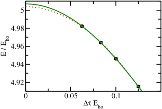
Figure 8: Illustration of the dependence of the PIGS energy on $\Delta\tau$ for the $(2,2)$ system. The symbols with error bar show the PIGS energy for $\tau=(E_{\rm{ho}})^{-1}$, obtained using the trial function given in Eqs. (118)-(120) with $\alpha=0.505$. The solid and dotted lines show second- and fourth-order fits to the energies (see text for details).

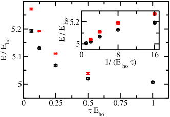
Figure 9: Illustration of the dependence of the PIGS energy on the propagation time $\tau$ for the $(2,2)$ system. The circles and crosses show the extrapolated $\Delta\tau=0$ energies with error bars (the fourth-order scheme is used), obtained using the trial function given in Eqs. (118)-(120) with $\alpha=0.505$ and $1$, respectively. The inset replots the energies as a function of $1/\tau$.

To analyze how close the $\tau=(E_{\rm{ho}})^{-1}$ energy is to the $\tau\rightarrow\infty$ limit, circles with error bars in Fig. 9 show the extrapolated energy, using the fourth-order scheme, of the $(2,2)$ system for various $\tau$; as before, $\alpha$ is set to $0.505$. As expected, the energy decreases with increasing $\tau$ and flattens out for large $\tau$. To better show how the energy behaves with increasing $\tau$, the inset replots the extrapolated $\Delta\tau=0$ energies with error bars as a function of $1/\tau$. It can be seen that the energies for the two smallest $1/\tau$ (two largest $\tau$) do not agree within error bars. This means that, strictly speaking, the large $\tau$ limit has not yet been reached. However, as discussed further below, going to larger $\tau$ is rather challenging because of the Fermi sign problem. This implies that, ultimately, the accuracy of the PIGS energy is limited, as already alluded to above, by the systematic error that originates from not going to the $\tau\to\infty$ limit and not by the statistical error bars. For the $N\geq 6$ systems, the computational time is chosen such that the statistical error is of the order of the estimated systematic error; the reasoning behind this is that a smaller statistical error would not allow one to gain more insight into the exact value of the energy.

For comparison, the crosses with error bars in the main part of Fig. 9 show the extrapolated $(2,2)$ PIGS energies for $\alpha=1$. These energies lie above those for $\alpha=0.505$ for all $\tau$, reflecting the fact that the trial function with $\alpha=0.505$ provides a better description of the $(2,2)$ system than the trial function with $\alpha=1$. The difference between the PIGS energies for the calculations with the two different $\alpha$ values decreases with increasing $\tau$, reflecting the fact that, in principle, any trial function that has finite overlap with the exact ground state wave function could be used. However, the better $\psi_{T}$, the smaller the resulting error bars.

To more systematically investigate the dependence of the PIGS energy, and correspondingly the speed of the convergence with increasing $\tau$, on $\alpha$, we fix $\tau$ at $0.125(E_{\rm{ho}})^{-1}$. These small $\tau$ calculations are computationally comparatively inexpensive and hence allow one to survey the $\alpha$ dependence more exhaustively. Ultimately, one needs, of course, to go to larger $\tau$. However, to find the best $\alpha$ (or more generally, the best trial function), it is often times sufficient to consider a relatively small $\tau$. Figure 10 shows the PIGS energy with error bars as a function of $\alpha^{-1}$ for $\tau=0.125(E_{\rm{ho}})^{-1}$. The lowest energy is obtained for $\alpha$ around $0.5$, confirming our choice of $\alpha$ based on the hyperspherical coordinate approach. This suggests that the optimal $\alpha$ could alternatively be determined iteratively. To this end, let us assume that the ground state energy is unknown. One would then chose an initial value of $\alpha$ to obtain a first PIGS energy estimate for small $\tau$. Using this (non-converged) PIGS energy, one would obtain an improved $\alpha$ value using Eq. (127) and perform another PIGS calculation. After a few iterations, the optimal $\alpha$ value would be found.

Figure 10: Illustration of the dependence of the PIGS energy for the $(2,2)$ system on the trial function parameter $\alpha$. The symbols show the extrapolated $\Delta\tau=0$ energies with error bars (the fourth-order scheme is used) for $\tau=0.125(E_{\rm{ho}})^{-1}$ as a function of $1/\alpha$, obtained using the trial function given in Eqs. (118)-(120).

As already alluded to, the Fermi sign problem limits the maximum propagation time $\tau$ that can be reached with a finite amount of computational resources. The symbols in Fig. 11 show the quantity $S$ [see Eq. (110)], which appears in the denominator of the expression for all observables, as a function of $\tau$ for the $(2,2)$ system for the trial function with $\alpha=0.505$. For this series of calculations, $\Delta\tau$ is fixed at $\Delta\tau=0.125(E_{\rm{ho}})^{-1}$, i.e., the number of time slices increases with increasing $\tau$. The solid line shows a fit to the data, demonstrating that $S$ decreases exponentially with increasing $\tau$ or, equivalently, increasing number of time slices. An $S$ value close to 1 indicates that the sign problem is irrelevant. The smaller $S$, the more severe the sign problem becomes. As a consequence, for a given $\tau$, there exists a maximum $\Delta\tau$ for which the calculation is feasible. For smaller $\Delta\tau$, the errors that originate from the sign problem are too large to be useful. For large $\tau$, the smallest $\Delta\tau$ that can be treated reliably might not be sufficiently small to allow for a reliable extrapolation to $\Delta\tau=0$. For the $(2,2)$ system, e.g., $\tau=(E_{\rm{ho}})^{-1}$ is a good compromise. The excited state contributions have, essentially, decayed and the extrapolation to the $\Delta\tau=0$ limit is reliable.

Figure 11: Symbols show the quantity $S$, Eq. (110), as a function of $\tau$ for the $(2,2)$ system. The error bars are smaller than the symbol size. The time step $\Delta\tau$ is fixed at $0.125(E_{\rm{ho}})^{-1}$. As a guide to the eye, the solid line connects consecutive data points.

In addition to the $(2,2)$ system, we treat the $(3,3)$, $(4,4)$, and $(5,5)$ systems using the $\alpha$ values determined from the known ground state energies via Eq. (127). The value of $\tau$ (see column 3 of Table 3) is chosen such that the estimated systematic error, due to the use of a finite $\tau$, is comparable to or smaller than the error of the extrapolated $\Delta\tau=0$ energy for this $\tau$ (see columns 4-6 of Table 3). As $N$ goes up, the propagation time $\tau$ is chosen to be smaller and smaller (see Table 3). The reason is that the simulations for larger $N$ are more computationally demanding since the Fermi sign problem becomes more severe with increasing $N$. This means that we are limited by the number of time slices and, correspondingly, the largest $\tau$ we can use. The number of time slices $2n+1$ considered in the $\Delta\tau\to 0$ extrapolation are chosen based on our detailed analysis of the $(2,2)$ system. Because of the relatively small $\tau$ considered, the energies reported for the $N/2=4$ and 5 systems should be regarded, within error bars, as variational upper bounds. Our $(3,3)$ energy agrees, within error bars, with the basis set expansion energy $E_{\rm{ECG}}$ but lies slightly below the diffusion Monte Carlo energy $E_{\rm{DMC}}$. For the $(4,4)$ and $(5,5)$ systems, the PIGS energies agree, within error bars, with $E_{\rm{ECG}}$ and $E_{\rm{DMC}}$. For the $(5,5)$ system, we performed an additional calculation using—as before—$\tau=0.125(E_{\rm{ho}})^{-1}$ but using an $\alpha$ value that is larger than that listed in Table 3, namely $\alpha=0.335$. The extrapolated $\Delta\tau=0$ PIGS energy is $16.22(14)E_{\rm{ho}}$, which agrees within error bars with our result listed in Table 3. The larger error bar reflects the fact that the larger $\alpha$ value provides a less good trial function.

The trial function used so far [see Eqs. (118)-(120)] contains a single adjustable parameter, namely $\alpha$, that primarily determines the correlations in the hyperradial degree of freedom. Our goal is now to design a trial function that provides an improved description of the hyperangular degrees of freedom. In doing so, we are guided by the analytically known wave function of the harmonically-trapped $(2,1)$ system with $(L,\Pi)=(0,+1)$ symmetry at unitarity [99]. The hyperangular part of the wave function that yields the lowest energy with $(0,+1)$ symmetry is proportional to

$$(1-\hat{P}_{12})\sin(\bar{s}_{0}(\theta_{1}-\pi/2))/\sin(2\theta_{1}),$$ (128)

where $\theta_{1}=\arcsin(r_{13}/(2\sqrt{\bar{R}}))$, $\bar{s}_{0}=2.166$, and $\bar{R}^{2}=\sum_{j<k}r_{jk}^{2}/N$. Application of $\hat{P}_{12}$ changes $\theta_{1}$ into $\theta_{2}$, where $\theta_{2}=\arcsin(r_{23}/(2\sqrt{\bar{R}}))$. The factor $\sin(\bar{s}_{0}(\theta_{1}-\pi/2))$ enhances the probability to find two particles at vanishing hyperangle $\theta_{1}$, i.e., at vanishing distance between the unlike particles 1 and 3. In the non-interacting limit, $\bar{s}_{0}$ is equal to $4$, which implies that the probability to find two particles at vanishing hyperangle $\theta_{1}$ vanishes. The quantities $\bar{R}$ and $\bar{s}_{0}$, which are defined by excluding the center-of-mass degrees of freedom, are related to $R$ and $s_{0}$, $\bar{R}^{2}=R^{2}-N(R_{\rm{cm}})^{2}$ and $\bar{s}_{0}=s_{0}-3/2$.

Motivated by the hyperangular wave function of the $(2,1)$ system with $(0,+1)$ symmetry at unitarity, we consider the following alternative form of the trial function,

$$\psi_{T}=f_{\rm{trap}}(\mathbf{R})\Phi_{\alpha,\beta,\gamma}(\mathbf{R}),$$ (129)

where

$$\Phi_{\alpha,\beta,\gamma}(\mathbf{R})=\frac{\bar{R}^{\alpha}}{(a_{\rm{ho}})^{\alpha+3N/2}}\hat{\mathcal{P}}\prod_{j=1}^{N/2}\frac{\sin[\beta(\theta_{j}-\pi/2)](\cos\theta_{j})^{\gamma+1}}{\sin(2\theta_{j})}$$ (130)

and $\theta_{j}=\arcsin(r_{j,N/2+j}/(2\sqrt{\bar{R}}))$. The factor $(\cos\theta_{j})^{\gamma+1}$ is introduced to increase the tunability of the trial function. As before, the optimal value of $\alpha$ is obtained by matching to the known hyperradial solution. This yields $\alpha=0.166$. The values of $\beta$ and $\gamma$, in contrast, are determined by performing PIGS simulations for small $\tau$.

Considering the $(2,2)$ system and using $\alpha=2.5091$, $\beta=1.1$, and $\gamma=2$, we obtain the extrapolated $\Delta\tau=0$ PIGS energy of $5.022(3)E_{\rm{ho}}$ for $\tau=0.0625(E_{\rm{ho}})^{-1}$. This energy is significantly lower than the PIGS energy of $5.193(4)E_{\rm{ho}}$ that we obtained using the correlation factor $\Phi_{\alpha}(\mathbf{R})$ for the same $\tau$. For $\tau=0.25(E_{\rm{ho}})^{-1}$, we obtain $5.011(8)E_{\rm{ho}}$, which agrees within error bars with the ground state energy $E_{\rm{ECG}}$ (see Table 3). Considering the $(3,3)$ system and using the trial parameters $\alpha=5.837$, $\beta=1.5$, and $\gamma=8$, we obtain the extrapolated $\Delta\tau=0$ PIGS energy of $8.357(8)E_{\rm{ho}}$ for $\tau=0.25(E_{\rm{ho}})^{-1}$. For comparison, the $(3,3)$ PIGS energy reported in Table 3 is for a larger $\tau$, namely $\tau=0.5(E_{\rm{ho}})^{-1}$. For the $(4,4)$ and $(5,5)$ systems, the trial function with the correlation factor $\Phi_{\alpha,\beta,\gamma}$ did not yield an improved energy compared to that for $\Phi_{\alpha}$. The reason could be that the trial parameters were not fully optimized or that the degrees of freedom of the larger systems are less well described by the trial function (e.g., that three- and higher-body correlations are needed).

In addition to the energies, we use the PIGS approach to calculate structural properties. The scaled pair distribution functions reported below are obtained for a finite $\Delta\tau$; no extrapolation to the $\Delta\tau=0$ limit was performed. To determine a suitable $\Delta\tau$, we consider the $(2,2)$ system and perform calculations for $\tau=0.25(E_{\rm{ho}})^{-1}$ using three different $\Delta\tau$, i.e., $\Delta\tau=0.25(E_{\rm{ho}})^{-1}$, $0.125(E_{\rm{ho}})^{-1}$, and $0.0625(E_{\rm{ho}})^{-1}$. We find that the scaled pair distribution function for $\Delta\tau=0.25(E_{\rm{ho}})^{-1}$ differs slightly from those for $\Delta\tau=0.125(E_{\rm{ho}})^{-1}$ and $\Delta\tau=0.0625(E_{\rm{ho}})^{-1}$. However, no visual difference is observed between the scaled pair distribution functions for $\Delta\tau=0.125(E_{\rm{ho}})^{-1}$ and $\Delta\tau=0.0625(E_{\rm{ho}})^{-1}$. Motivated by this observation, we calculate the scaled pair distribution functions for the spin-balanced systems with $N/2\leq 5$ using $\Delta\tau=0.125(E_{\rm{ho}})^{-1}$. The propagation times and trial functions are the same as those used to obtain the energies reported in Table 3.

Solid lines in Figs. 12(a)-12(d) show the resulting scaled pair distribution function for the spin-balanced systems with $N=4-10$. For comparison, the dashed lines show the scaled pair distribution function obtained from basis set calculations for an attractive two-body Gaussian potential with infinitely large $s$-wave scattering length and effective range of approximately $0.12a_{\rm{ho}}$ (the range is $0.06a_{\rm{ho}}$) [97]. The Gaussian potential used supports exactly one zero-energy two-body bound state in free space. If the effective range were taken to zero, the two different approaches should yield the same result. As can be seen from Fig. 12, the zero-range results deviate a bit from the finite-range results at small interparticle distances; in particular, the scaled pair distribution functions take a finite value for vanishing interparticle distance if the zero-range interaction model is used and go to zero if the finite-range interaction model is used. At larger interparticle distances, the agreement between the dashed and solid lines is quite good, suggesting that the PIGS scaled pair distribution functions are, indeed, quite well converged for $r\gtrsim 0.5a_{\rm{ho}}$.

To check the convergence at small interparticle distances, we report the contact $C$ obtained from the $r=0$ value of the scaled pair distribution function [100],

$$C=4\pi n_{1}n_{2}\lim_{r\to 0}4\pi r^{2}P_{12}(r).$$ (131)

The resulting contacts are summarized in Table 4. The contact calculated by the PIGS approach is, for all $N$ considered, larger than the contact calculated by extrapolating basis set expansion results (namely, the slope of the energy with respect to the inverse of the $s$-wave scattering length) for finite-range interactions to the zero-range limit. As $N/2$ increases from $2$ to $5$, the difference between the two sets of results increases from about two to about six standard deviations. The numerical determination of the contact through the scaled pair distribution function is, in general, quite challenging since the contact probes a small portion of the Hilbert space. As a consequence, the convergence of the contact can be slow. It is presently unclear which set of results is more reliable and if, possibly, the errorbars of the results obtained by either of the two methods was underestimated: the basis set expansion results may be “contaminated” by basis set extrapolation and zero-range extrapolation errors while the PIGS results may be “contaminated” by finite propagation time and finite time step errors.

Table 4: Contact for spin-balanced two-component Fermi gas ($N/2\leq 5$) with zero-range interactions at unitarity. Column 2 reports the value of the contact $C_{\rm{PIGS}}$ obtained from our PIGS simulations with $\Delta\tau=0.125(E_{\rm{ho}})^{-1}$. The error reported does not include the systematic error introduced by not extrapolating to zero $\Delta\tau$. Column 3 shows the contact $C_{\rm{ECG}}$ from the literature, obtained by extrapolating the contact obtained by the ECG approach for finite-range interactions to the zero-range limit [97].

$(n_{1},n_{2})$	$C_{\rm{PIGS}}a_{\rm{ho}}$	$C_{\rm{ECG}}a_{\rm{ho}}$
(2,2)	25.91(6)	25.74(1)
(3,3)	42.26(5)	40.39(8)
(4,4)	59.5(2)	55.4(5)
(5,5)	79.3(3)	72.3(8)

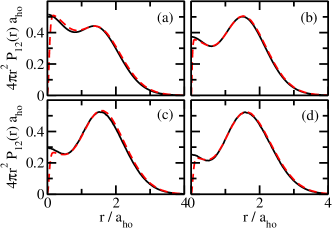
Figure 12: Scaled pair distribution functions $4\pi r^{2}P_{12}(r)$ for the (a) $(2,2)$, (b) $(3,3)$, (c) $(4,4)$, and (d) $(5,5)$ systems at unitarity. The solid lines show our PIGS results for the model Hamiltonian with two-body zero-range interactions. The results are obtained using the propagation times and trial function parameters listed in Table 3. The imaginary time step is set to $\Delta\tau=0.125(E_{\rm{ho}})^{-1}$. For comparison, the dashed lines show basis set expansion based results [97] for an attractive two-body Gaussian interaction with finite effective range (see text for details).

5.3 Non-interacting Fermi gas with a single impurity

This section considers a non-interacting Fermi gas with a single impurity, i.e., the $(n_{1},n_{2})=(N-1,1)$ system with $N=3-5$. In a zeroth-order approximation, one can think of this system as consisting of one up-down pair and $N-2$ unpaired spin-up atoms. Of course, this picture needs to be refined to account for the fact that the system contains $N-1$ identical fermions and for the fact that the presence of additional spin-up fermions “disturbs” the single pair. Nevertheless, the simple picture correctly suggests that the ground state of the $(N-1,1)$ system does not have $(L,\Pi)=(0,+1)$ symmetry. Rather, the ground state of the $(2,1)$, $(3,1)$ and $(4,1)$ systems has $(L,\Pi)=(1,-1)$, $(1,+1)$ and $(0,-1)$ symmetry [99, 101, 102]. Roughly, this can be understood by realizing that the $(2,1)$, $(3,1)$ and $(4,1)$ systems contain one, two and three unpaired spin-up atoms, each of which carry one quantum of angular momentum (the $p$-shell is being filled). Thus, due to the angular momentum carried by the single unpaired spin-up atom the $(2,1)$ system has $(1,-1)$ symmetry. In the $(3,1)$ system, the angular momenta of each of the two unpaired atoms can couple to an angular momentum $0$, $1$, or $2$, with the parity being even. The $(1,+1)$ channel turns out to have the lowest energy [102]. Last, in the $(4,1)$ system, the angular momenta of each of the three unpaired atoms can couple to an angular momentum $0$, $1$, $2$, or $3$, with the parity being odd. Consistent with the idea of a closed shell configuration, the $(0,-1)$ channel turns out to have the lowest energy.

As our first application of the PIGS approach to spin-imbalanced systems, we treat the $(2,1)$ system with $(L,\Pi)=(0,+1)$ symmetry. This application illustrates that the PIGS approach can be used to describe the energetically lowest-lying state (not the “absolute ground state”) of a given symmetry. Following the logic that motivated the trial function given in Eqs. (118)-(120), we write

$$\psi_{T}(\mathbf{R})=f_{\rm{trap}}(\mathbf{R})\Phi_{\alpha^{\prime}}(\mathbf{R}),$$ (132)

where

$$\Phi_{\alpha^{\prime}}(\mathbf{R})=(a_{\rm{ho}})^{-\alpha^{\prime}(N-2)-3N/2+1}\hat{\mathcal{P}}\left(\frac{\prod_{j=2}^{N-1}(r_{j,N})^{\alpha^{\prime}}}{r_{1,N}}\right).$$ (133)

Using a relatively small $\tau$, namely $\tau=0.25(E_{\rm{ho}})^{-1}$, Table 5 shows the extrapolated $\Delta\tau=0$ energy. It lies about six sigma above the exact energy obtained within the hyperspherical coordinate approach [99]. If we repeated the calculation for larger $\tau$, we would expect to obtain a PIGS energy closer to the exact energy. To prove that the lowest $(0,+1)$ energy can be obtained exactly within the PIGS approach, i.e., to prove that the PIGS approach does, indeed, preserve the symmetry of the trial function, we use the exact (analytically known) eigen state [99] as the trial function. The resulting extrapolated $\Delta\tau=0$ energy (see Table 5) agrees to within error bars with the exact energy.

As a proof-of-principle, we apply the PIGS approach to the $(2,1)$ system with $(L,\Pi)=(1,-1)$ symmetry at unitarity. Knowing that the orbital angular momentum is carried by the Jacobi vector $\mathbf{r}_{13,2}$ when particles 1 and 3 form a pair and by the Jacobi vector $\mathbf{r}_{23,1}$ when particles 2 and 3 form a pair [99, 101], we write

$$\psi_{T}(\mathbf{R})=(a_{\rm{ho}})^{-9/2}f_{\rm{trap}}(\mathbf{R})\left(\frac{\bar{R}}{a_{\rm{ho}}}\right)^{\alpha}{\hat{\cal{P}}}\left(\frac{x_{13,2}}{r_{13,2}}\right).$$ (134)

Owing to the three-fold degeneracy of $L=1$ states, alternatively one can use $y_{13,2}$ or $z_{13,2}$ instead of $x_{13,2}$. In an equivalent formulation, the term $x_{13,2}/r_{13,2}$ in Eq. (134) is replaced by $Y_{1,m_{l}}(\hat{\mathbf{r}}_{13,2})$, where $Y_{1,m_{l}}$ denotes the spherical harmonic and $m_{l}$ can take the values $\pm 1$ and $0$. Since the spherical harmonics with $m_{l}\neq 0$ are complex, spherical harmonics are less convenient from a numerical/implementation perspective than the real version used in Eq. (134). Using Eq. (134) with $\tau=0.5(E_{\rm{ho}})^{-1}$, we find the extrapolated $\Delta\tau=0$ energy $E_{\rm{PIGS}}=4.276(9)E_{\rm{ho}}$, which agrees, within error bars, with the exact zero-range energy from Ref. [99] (see row 3 of Table 5).

The above trial function can be extended to the $(3,1)$ system. Assuming the formation of a pair consisting of atoms 1 and 4, one quantum of orbital angular momentum each is assumed to be carried by the vectors $\mathbf{r}_{14,2}$ and $\mathbf{r}_{14,3}$. Coupling $Y_{1,m_{1}}(\mathbf{r}_{14,2})$ and $Y_{1,m_{2}}(\mathbf{r}_{14,3})$ such that the resulting function has $(L,\Pi)=(1,-1)$ symmetry, we obtain the desired correlation factor. Since we prefer to work with real quantities, we write

$$\psi_{T}(\mathbf{R})=(a_{\rm{ho}})^{-6}f_{\rm{trap}}(\mathbf{R})\left(\frac{\bar{R}}{a_{\rm{ho}}}\right)^{\alpha}\hat{\mathcal{P}}\left(\frac{(\mathbf{r}_{14,2}\times\mathbf{r}_{14,3})\cdot{\hat{\mathbf{z}}}}{r_{14,2}r_{14,3}}\right),$$ (135)

where the dot product serves to select the $z$-component of the vector that results when taking the cross product. Instead of the $z$-component, the $x$- or $y$-components can be used. For the $(4,1)$ system, we use

$$\psi_{T}(\mathbf{R})=(a_{\rm{ho}})^{-15/2}f_{\rm{trap}}(\mathbf{R})\left(\frac{\bar{R}}{a_{\rm{ho}}}\right)^{\alpha}\hat{\mathcal{P}}\left(\frac{(\mathbf{r}_{15,2}\times\mathbf{r}_{15,3})\cdot{\mathbf{r}_{15,4}}}{r_{15,2}r_{15,3}r_{15,4}}\right),$$ (136)

which has the desired $(L,\Pi)=(0,-1)$ symmetry. Alternatively, one could use

$$\psi_{T}(\mathbf{R})=(a_{\rm{ho}})^{-21/2}f_{\rm{trap}}(\mathbf{R})\left(\frac{\bar{R}}{a_{\rm{ho}}}\right)^{\alpha}\hat{\mathcal{P}}\left((\mathbf{r}_{15,2}\times\mathbf{r}_{15,3})\cdot{\mathbf{r}_{15,4}}\right).$$ (137)

The resulting extrapolated $\Delta\tau=0$ energies for the $(3,1)$ and $(4,1)$ systems are reported in Table 6. The $(3,1)$ PIGS energy deviates by two sigma from the highly-accurate basis set expansion energy $E_{\rm{ECG}}$. The small disagreement may be due to the fact that $\tau$ is not quite large enough or that the error bar of the extrapolated energy is, in fact, slightly larger than what is reported in Table 6. The $(4,1)$ PIGS energies for $\tau=0.5(E_{\rm{ho}})^{-1}$ and $\tau=(E_{\rm{ho}})^{-1}$ agree, within error bars, with the energy $E_{\rm{DMC}}$. Since the diffusion Monte Carlo energy was not extrapolated to the zero-range limit, the true zero-range energy is probably somewhat smaller than $E_{\rm{DMC}}$.

Table 5: Spin-imbalanced fermionic $(2,1)$ system with zero-range interactions at unitarity. Columns 2, 3, and 4 report the propagation time, the $n$ used (the number of time slices is 2$n$+1), and the trial function employed for two different symmetries (see column 1). Column 5 shows the resulting PIGS energy with error bars. For the $(0,+1)$ channel, no extrapolation to the $\Delta\tau=0$ limit was performed. For the $(1,-1)$ channel, a second-order extrapolation was used. For comparison, column 6 shows the exact zero-range energies obtained using the formalism developed in Ref. [99].

$(L,\Pi)$	$\tau E_{\rm{ho}}$	$n$ used	trial function	$E_{\rm{PIGS}}/E_{\rm{ho}}$	$E_{\rm{exact}}/E_{\rm{ho}}$
$(0,+1)$	0.25	4	Eq. (132), $\alpha=1.66622$	4.687(4)	4.66622
$(0,+1)$	0.25	4	Eq. (128)	4.676(10)	4.66622
$(1,-1)$	0.5	2,4	Eq. (134), $\alpha=0.772724$	4.276(9)	4.27272

Table 6: Spin-imbalanced fermionic $(N-1,1)$ system ($N=4$ and $5$) with zero-range interactions at unitarity. Column 1 lists the $(N-1,1)$ system considered. The symmetry of the ground state is reported in column 2. Columns 3, 4, 5, and 6 report the propagation time, the $n$ used (2$n$+1 is the number of time slices included in the extrapolation of the energy to $\Delta\tau=0$), the value of $\alpha$, and the equation number of the trial function used. Column 7 shows the resulting extrapolated $\Delta\tau=0$ PIGS energy with error bars, obtained using a second-order extrapolation. For comparison, column 8 reports energies obtained using the explicitly correlated Gaussian approach [103, 102]; the energies, which are denoted by $E_{\rm{ECG}}$, are obtained by extrapolating a series of finite-range energies to the zero-range limit. Column 9 reports the $(4,1)$ energy $E_{\rm{DMC}}$ for a square-well potential with range $r_{0}=0.01a_{\rm{ho}}$ obtained using the diffusion Monte Carlo method [104]; no extrapolation to the zero-range limit was done. The uncertainties for the ECG and DMC calculations are, according to Refs. [103, 102, 104], in the last digit reported.

	$(L,\Pi)$	$\tau E_{\rm{ho}}$	$n$	$\alpha$	$\psi_{T}$	$E_{\rm{PIGS}}/E_{\rm{ho}}$	$E_{\rm{ECG}}/E_{\rm{ho}}$	$E_{\rm{DMC}}/E_{\rm{ho}}$
$(3,1)$	$(1,+1)$	0.5	4, 8	0.791	(135)	6.60(1)	6.5819
$(4,1)$	$(0,-1)$	0.5	2, 4	0.667	(136)	8.93(7)	8.95	8.93
$(4,1)$	$(0,-1)$	1	4, 8	0	(137)	8.92(4)	8.95	8.93

In addition to the energy, we determine the contact $C$ from the $r=0$ behavior of the scaled pair distribution function [see Eq. (131)]. In general, the convergence rate of the energy and that of other observables can be different. For the case at hand, namely the contact, this can be understood by realizing that only a small fraction of the wave function amplitude is located at small $r$. Thus, while the energies shown in Table 6 appear to be converged, the contact may not be. Indeed, this is what we find. Figure 13 shows the contact of the $(3,1)$ system as a function of $\tau^{-1}$. The calculations are performed for $\Delta\tau=0.125(E_{\rm{ho}})^{-1}$. The contacts for the two largest $\tau$ values considered differ by roughly 2%. For even larger $\tau$, the curve should flatten out. Thus, we can interpret our calculations as providing a lower bound on $C$, $C\geq 10.7(a_{\rm{ho}})^{-1}$. Indeed, calculations that employ a correlated Gaussian basis set yield a contact of $C=10.84(2)(a_{\rm{ho}})^{-1}$ (see the dashed horizontal line in Fig. 13), which is close to the PIGS contact for the largest $\tau$ considered. For $\tau=0.5(E_{\rm{ho}})^{-1}$, we performed an additional calculation for a smaller $\Delta\tau$, i.e., for $\Delta\tau=0.0625(E_{\rm{ho}})^{-1}$. The results for $\Delta\tau=0.125(E_{\rm{ho}})^{-1}$ and $\Delta\tau=0.0625(E_{\rm{ho}})^{-1}$ differ by 0.4%, which is small compared to the error introduced by not extrapolating to the $\tau=\infty$ limit.

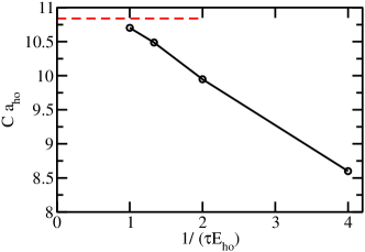
Figure 13: Symbols show the contact $C$ of the $(3,1)$ system as a function of $\tau^{-1}$. The time step $\Delta\tau$ is fixed at $0.125(E_{\rm{ho}})^{-1}$. As a guide to the eye, the symbols are connected by a solid line. For comparison, the dashed horizontal line shows the contact $C=10.84(2)(a_{\rm{ho}})^{-1}$, obtained by extrapolating basis set expansion results for finite-range interactions to the zero-range limit.

6 Summary and outlook

This article provided a detailed introduction to the path integral ground state Monte Carlo (PIGS) algorithm. Implementation details and convergence properties were discussed using general arguments and subsequently illustrated for selected systems and observables. While the primary focus was on the PIGS approach, several aspects are applicable more broadly. For example, the discussion of the error analysis is relevant to essentially all Monte Carlo algorithms and many features of the path generation apply also to the finite-temperature path integral Monte Carlo approach.

The PIGS algorithm takes a trial function, which is selected by the simulator, and propagates it in imaginary time. For sufficiently large imaginary time $\tau$, the lowest eigen state of the system Hamiltonian, which has finite overlap with the trial function, is being projected out. A crucial question is how to assess whether the resulting eigen energy and other observables are truly converged. This question is particularly pressing for fermionic systems, for which the largest $\tau$ considered is restricted by numerical instabilities due to the Fermi sign problem. In the absence of identical fermions, the convergence analysis is relatively simple since there are essentially no restrictions on the $\tau$ that can be considered. The applications to fermions considered in this tutorial employed a multi-faceted approach to the convergence analysis. For small systems, comparisons with established literature results were used as a benchmark. For larger systems, an analysis of the error bars was used to establish where the Fermi sign problem sets in. For $\tau$ not noticably impacted by the Fermi sign problem, the resulting energies, extrapolated to the infinite time slice limit, provided variational upper bounds. Additionally, the calculations were performed for different trial functions and the runs were checked for consistency. Ultimately, there is no guarantee that the resulting observables are not biased by the trial function. However, the various checks provide one with tools for (roughly) estimating and minimizing the variational bias.

The sample applications presented concern strongly-correlated Fermi gases. In cold atom experiments, the two-body van der Waals length is typically much smaller than the average interparticle spacing and the two-body $s$-wave scattering length (for two-component Fermi systems, this is the interspecies (and not the intraspecies) scattering length). Thus, cold atom systems realize, to a very good approximation, idealized systems in which the two-body interaction range is zero. From a theoretical point of view, a vanishing two-body range is particularly interesting as this implies that the range drops out of the problem. For infinitely large two-body $s$-wave scattering length, e.g., the system exhibits a scale invariance, reflecting underlying symmetries of the Hamiltonian. While scale-invariance based arguments and formulations have led to a great deal of insight into these paradigmatic, strongly-correlated systems, few analytical or numerical techniques exist that can reliably predict the energy, Tan contact, superfluid fraction, or other observables. The PIGS approach treats two-body zero-range interactions by building the exact two-body Bethe-Peierls boundary condition into the propagator using the pair product approximation. For fermions, the treatment is limited to small number of particles since the Fermi sign problem becomes exponentially more severe with increasing number of identical fermions. The system sizes considered in this article are the same as those that have been treated by the explicitly correlated Gaussian basis set expansion approach [97]. For both (the PIGS and basis set expansion approach), the computational effort increases tremendously as $N$ is increased beyond what is considered in this article.

Future applications of the PIGS approach to systems with zero-range interactions may include unequal-mass two-component Fermi gases, Fermi gases in non-spherically symmetric external traps (including effectively low-dimensional systems), or Bose droplets without and with an impurity. These applications can be tackled with the technology already developed. An interesting and challenging future development is the treatment of spin-orbit coupled systems, where the spatial degrees of freedom are coupled to the spin degrees of freedom. It will be interesting to marry the treatment of spin degrees of freedom with the use of two-body zero-range interactions.

7 Acknowledgments

We are grateful to Xiangyu Yin for providing the scaled pair distribution functions from Ref. [97] (dashed lines in Fig. 12) in tabular form. Support by the National Science Foundation (NSF) through Grant No. PHY-1415112 is gratefully acknowledged. This work used the Extreme Science and Engineering Discovery Environment (XSEDE), which is supported by NSF Grant No. OCI-1053575, and the WSU HPC.

References

- Binder [1986] K. Binder, Monte Carlo Methods in Statistical Physics (Springer Berlin, Heidelberg, 1986).
- Hetényi et al. [1999] B. Hetényi, E. Rabani, and B. J. Berne, “Path-integral diffusion Monte Carlo: Calculation of observables of many-body systems in the ground state,” J. Chem. Phys. 110, 6143 (1999).
- Sarsa et al. [2000] A. Sarsa, K. E. Schmidt, and W. R. Magro, “A path integral ground state method,” J. Chem. Phys. 113, 1366 (2000).
- Cuervo et al. [2005] J. E. Cuervo, P.-N. Roy, and M. Boninsegni, “Path integral ground state with a fourth-order propagator: Application to condensed helium,” J. Chem. Phys. 122, 114504 (2005).
- Rota et al. [2010] R. Rota, J. Casulleras, F. Mazzanti, and J. Boronat, “High-order time expansion path integral ground state,” Phys. Rev. E 81, 016707 (2010).
- Ceperley [1995] D. M. Ceperley, “Path integrals in the theory of condensed helium,” Rev. Mod. Phys. 67, 279 (1995).
- Hammond et al. [1994] B. L. Hammond, W. A. Lester Jr., and P. J. Reynolds, Monte Carlo Methods in Ab Initio Quantum Chemistry, Lecture and Course Notes In Chemistry Series, Vol. 1 (World Scientific, Singapore, 1994).
- Press [2007] W. Press, Numerical Recipes 3rd Ed.: The Art of Scientific Computing (Cambridge University Press, Cambridge, UK, 2007).
- Boninsegni [2005] M. Boninsegni, “Permutation Sampling in Path Integral Monte Carlo,” J. Low Temp. Phys. 141, 27 (2005).
- Whitley et al. [2009] H. D. Whitley, J. L. DuBois, and K. B. Whaley, “Spectral shifts and helium configurations in 4HeN-tetracene clusters,” J. Chem. Phys. 131, 124514 (2009).
- Guardiola [1988] R. Guardiola, “Monte Carlo Techniques in the Many Body Problem,” in First International Course on Condensed Matter, edited by D. P. S. Rosati and G. Violini (World Scientific, Singapore, 1988).
- Casulleras and Boronat [1995] J. Casulleras and J. Boronat, “Unbiased estimators in quantum Monte Carlo methods: Application to liquid ,” Phys. Rev. B 52, 3654 (1995).
- Reynolds et al. [1986] P. J. Reynolds, R. N. Barnett, B. L. Hammond, and W. A. Lester Jr., “Molecular physics and chemistry applications of quantum Monte Carlo,” J. Stat. Phys. 43, 1017 (1986).
- Moroni and Boninsegni [2004] S. Moroni and M. Boninsegni, “Condensate Fraction in Liquid 4He,” J. Low Temp. Phys. 136, 129 (2004).
- Herdman et al. [2014] C. M. Herdman, S. Inglis, P.-N. Roy, R. G. Melko, and A. Del Maestro, “Path-integral Monte Carlo method for Rényi entanglement entropies,” Phys. Rev. E 90, 013308 (2014).
- Hastings et al. [2010] M. B. Hastings, I. González, A. B. Kallin, and R. G. Melko, “Measuring Renyi Entanglement Entropy in Quantum Monte Carlo Simulations,” Phys. Rev. Lett. 104, 157201 (2010).
- Galli and Reatto [2004a] D. E. Galli and L. Reatto, “Disorder Phenomena in Quantum Solids with Vacancies,” J. Low Temp. Phys. 134, 121 (2004a).
- Vitali et al. [2008] E. Vitali, M. Rossi, F. Tramonto, D. E. Galli, and L. Reatto, “Path-integral ground-state Monte Carlo study of two-dimensional solid ,” Phys. Rev. B 77, 180505 (2008).
- Rossi et al. [2012] M. Rossi, E. Vitali, L. Reatto, and D. E. Galli, “Microscopic characterization of overpressurized superfluid 4He,” Phys. Rev. B 85, 014525 (2012).
- Galli et al. [2007] D. E. Galli, L. Reatto, and W. M. Saslow, “Bounds for the superfluid fraction from exact quantum Monte Carlo local densities,” Phys. Rev. B 76, 052503 (2007).
- Rossi et al. [2010] M. Rossi, E. Vitali, D. E. Galli, and L. Reatto, “Quantum dislocations: the fate of multiple vacancies in two-dimensional solid 4He,” J. Phys. C 22, 145401 (2010).
- Nava et al. [2013] M. Nava, D. E. Galli, S. Moroni, and E. Vitali, “Dynamic structure factor for 3He in two dimensions,” Phys. Rev. B 87, 144506 (2013).
- Arrigoni et al. [2013] F. Arrigoni, E. Vitali, D. E. Galli, and L. Reatto, “Excitation spectrum in two-dimensional superfluid 4He,” Low Temp. Phys. 39, 793 (2013).
- Carleo et al. [2009] G. Carleo, S. Moroni, and S. Baroni, “Zero-temperature dynamics of solid from quantum Monte Carlo simulations,” Phys. Rev. B 80, 094301 (2009).
- Galli and Reatto [2004b] D. E. Galli and L. Reatto, “The Shadow Path Integral Ground State Method: Study of Confined Solid 4He,” J. Low Temp. Phys. 136, 343 (2004b).
- Nava et al. [2012a] M. Nava, D. E. Galli, M. W. Cole, and L. Reatto, “Adsorption of He isotopes on fluorographene and graphane: Fluid and superfluid phases from quantum Monte Carlo calculations,” Phys. Rev. B 86, 174509 (2012a).
- Turnbull and Boninsegni [2005] J. D. Turnbull and M. Boninsegni, “Adsorption of para-hydrogen on fullerenes,” Phys. Rev. B 71, 205421 (2005).
- Turnbull and Boninsegni [2007] J. Turnbull and M. Boninsegni, “Molecular hydrogen isotopes adsorbed on krypton-preplated graphite,” Phys. Rev. B 76, 104524 (2007).
- Cuervo and Roy [2006] J. E. Cuervo and P.-N. Roy, “Path integral ground state study of finite-size systems: Application to small (parahydrogen)N (= 2–20) clusters,” J. Chem. Phys. 125, 124314 (2006).
- Cuervo and Roy [2008] J. E. Cuervo and P.-N. Roy, “On the solid- and liquidlike nature of quantum clusters in their ground state,” J. Chem. Phys. 128, 224509 (2008).
- Cuervo and Roy [2009] J. E. Cuervo and P.-N. Roy, “Weakly bound complexes trapped in quantum matrices: Structure, energetics, and isomer coexistence in (para-H2)N(ortho-D2)3 clusters,” J. Chem. Phys. 131, 114302 (2009).
- Rossi and Salasnich [2013] M. Rossi and L. Salasnich, “Path-integral ground state and superfluid hydrodynamics of a bosonic gas of hard spheres,” Phys. Rev. A 88, 053617 (2013).
- Rota et al. [2013] R. Rota, F. Tramonto, D. E. Galli, and S. Giorgini, “Quantum Monte Carlo study of the dynamic structure factor in the gas and crystal phase of hard-sphere bosons,” Phys. Rev. B 88, 214505 (2013).
- Macia et al. [2012] A. Macia, D. Hufnagl, F. Mazzanti, J. Boronat, and R. E. Zillich, “Excitations and Stripe Phase Formation in a Two-Dimensional Dipolar Bose Gas with Tilted Polarization,” Phys. Rev. Lett. 109, 235307 (2012).
- Moroni and Boninsegni [2014] S. Moroni and M. Boninsegni, “Coexistence, Interfacial Energy, and the Fate of Microemulsions of 2D Dipolar Bosons,” Phys. Rev. Lett. 113, 240407 (2014).
- Pilati and Troyer [2012] S. Pilati and M. Troyer, “Bosonic Superfluid-Insulator Transition in Continuous Space,” Phys. Rev. Lett. 108, 155301 (2012).
- Giorgini et al. [2008] S. Giorgini, L. P. Pitaevskii, and S. Stringari, “Theory of ultracold atomic Fermi gases,” Rev. Mod. Phys. 80, 1215 (2008).
- Blume [2012] D. Blume, “Few-body physics with ultracold atomic and molecular systems in traps,” Rep. Prog. Phys. 75, 046401 (2012).
- Levinsen et al. [2017] J. Levinsen, P. Massignan, S. Endo, and M. M. Parish, “Universality of the unitary Fermi gas: a few-body perspective,” J. Phys. B 50, 072001 (2017).
- Heiselberg [2001] H. Heiselberg, “Fermi systems with long scattering lengths,” Phys. Rev. A 63, 043606 (2001).
- Werner and Castin [2012] F. Werner and Y. Castin, “General relations for quantum gases in two and three dimensions: Two-component fermions,” Phys. Rev. A 86, 013626 (2012).
- Casula et al. [2008] M. Casula, D. M. Ceperley, and E. J. Mueller, “Quantum Monte Carlo study of one-dimensional trapped fermions with attractive contact interactions,” Phys. Rev. A 78, 033607 (2008).
- Piatecki and Krauth [2014] S. Piatecki and W. Krauth, “Efimov-driven phase transitions of the unitary Bose gas,” Nat. Comm. 5, 3503 (2014).
- Pessoa et al. [2015a] R. Pessoa, S. A. Vitiello, and K. E. Schmidt, “Monte Carlo Calculations for Fermi Gases in the Unitary Limit with a Zero-Range Interaction,” J. Low Temp. Phys. 180, 168 (2015a).
- Yan and Blume [2015a] Y. Yan and D. Blume, “Incorporating exact two-body propagators for zero-range interactions into -body Monte Carlo simulations,” Phys. Rev. A 91, 043607 (2015a).
- Pessoa et al. [2015b] R. Pessoa, S. Gandolfi, S. A. Vitiello, and K. E. Schmidt, “Contact interaction in a unitary ultracold Fermi gas,” Phys. Rev. A 92, 063625 (2015b).
- Ardila and Giorgini [2016] L. A. Peña Ardila and S. Giorgini, “Bose polaron problem: Effect of mass imbalance on binding energy,” Phys. Rev. A 94, 063640 (2016).
- Parisi and Giorgini [2017] L. Parisi and S. Giorgini, “Quantum Monte Carlo study of the Bose-polaron problem in a one-dimensional gas with contact interactions,” Phys. Rev. A 95, 023619 (2017).
- Lin et al. [2011] Y.-J. Lin, K. Jiménez-García, and I. B. Spielman, “Spin-orbit-coupled Bose-Einstein condensates,” Nature 471, 83 (2011).
- Dalibard et al. [2011] J. Dalibard, F. Gerbier, G. Juzeliūnas, and P. Öhberg, “Colloquium: Artificial gauge potentials for neutral atoms,” Rev. Mod. Phys. 83, 1523 (2011).
- Zhai [2015] H. Zhai, “Degenerate quantum gases with spin-orbit coupling: a review,” Rep. Prog. Phys. 78, 026001 (2015).
- Carlson et al. [1987] J. Carlson, K. E. Schmidt, and M. H. Kalos, “Microscopic calculations of with realistic interactions,” Phys. Rev. C 36, 27 (1987).
- Shumway and Ceperley [2001] J. Shumway and D. M. Ceperley, “Quantum Monte Carlo treatment of elastic exciton-exciton scattering,” Phys. Rev. B 63, 165209 (2001).
- Shumway and Ceperley [2005] J. Shumway and D. M. Ceperley, “Quantum Monte Carlo simulations of exciton condensates,” Solid State Commun. 134, 19 (2005).
- Nollett et al. [2007] K. M. Nollett, S. C. Pieper, R. B. Wiringa, J. Carlson, and G. M. Hale, “Quantum Monte Carlo Calculations of Neutron- Scattering,” Phys. Rev. Lett. 99, 022502 (2007).
- Magnus [1954] W. Magnus, “On the exponential solution of differential equations for a linear operator,” Commun. Pure Appl. Math. 7, 649 (1954).
- Reynolds et al. [1982] P. J. Reynolds, D. M. Ceperley, B. J. Alder, and W. A. Lester Jr., “Fixed-node quantum Monte Carlo for molecules,” J. Chem. Phys. 77, 5593 (1982).
- Ceperley and Alder [1980] D. M. Ceperley and B. J. Alder, “Ground State of the Electron Gas by a Stochastic Method,” Phys. Rev. Lett. 45, 566 (1980).
- Krauth [2006] W. Krauth, Statistical Mechanics: Algorithms and Computations, Oxford Master Series in Physics (Oxford University Press, Oxford, UK, 2006).
- Gaveau and Schulman [1986] B. Gaveau and L. S. Schulman, “Explicit time-dependent Schrödinger propagators,” J. Phys. A 19, 1833 (1986).
- Lawande and Bhagwat [1988] S. V. Lawande and K. V. Bhagwat, “Feynman propagator for the -function potential,” Phys. Lett. A 131, 8 (1988).
- Blinder [1988] S. M. Blinder, “Green’s function and propagator for the one-dimensional -function potential,” Phys. Rev. A 37, 973 (1988).
- Wódkiewicz [1991] K. Wódkiewicz, “Fermi pseudopotential in arbitrary dimensions,” Phys. Rev. A 43, 68 (1991).
- Chandler and Wolynes [1981] D. Chandler and P. G. Wolynes, “Exploiting the isomorphism between quantum theory and classical statistical mechanics of polyatomic fluids,” J. Chem. Phys. 74, 4078 (1981).
- Trotter [1959] H. F. Trotter, “On the product of semi-groups of operators,” Proc. Amer. Math. Soc. 10, 545 (1959).
- Rossmann [2006] W. Rossmann, Lie Groups: An Introduction Through Linear Groups, Oxford graduate texts in mathematics (Oxford University Press, Oxford, UK, 2006).
- Chin [1997] S. A. Chin, “Symplectic integrators from composite operator factorizations,” Phys. Lett. A 226, 344 (1997).
- Suzuki [1995] M. Suzuki, “Hybrid exponential product formulas for unbounded operators with possible applications to Monte Carlo simulations,” Phys. Lett. A 201, 425 (1995).
- Barker [1979] J. A. Barker, “A quantum-statistical Monte Carlo method; path integrals with boundary conditions,” J. Chem. Phys. 70, 2914 (1979).
- Cao and Berne [1992] J. Cao and B. J. Berne, “A new quantum propagator for hard sphere and cavity systems,” J. Chem. Phys. 97, 2382 (1992).
- Chin [2005] S. A. Chin, “Structure of positive decompositions of exponential operators,” Phys. Rev. E 71, 016703 (2005).
- Zillich et al. [2010] R. E. Zillich, J. M. Mayrhofer, and S. A. Chin, “Extrapolated high-order propagators for path integral Monte Carlo simulations,” J. Chem. Phys. 132, 044103 (2010).
- Nava et al. [2012b] M. Nava, D. E. Galli, M. W. Cole, and L. Reatto, “Adsorption of He isotopes on fluorographene and graphane: Fluid and superfluid phases from quantum Monte Carlo calculations,” Phys. Rev. B 86, 174509 (2012b).
- Huang and Yang [1957] K. Huang and C. N. Yang, “Quantum-Mechanical Many-Body Problem with Hard-Sphere Interaction,” Phys. Rev. 105, 767 (1957).
- Yan and Blume [2016] Y. Yan and D. Blume, “Path-Integral Monte Carlo Determination of the Fourth-Order Virial Coefficient for a Unitary Two-Component Fermi Gas with Zero-Range Interactions,” Phys. Rev. Lett. 116, 230401 (2016).
- Bernard et al. [2009] E. P. Bernard, W. Krauth, and D. B. Wilson, “Event-chain Monte Carlo algorithms for hard-sphere systems,” Phys. Rev. E 80, 056704 (2009).
- Berg [2004] B. Berg, Markov Chain Monte Carlo Simulations and Their Statistical Analysis: With Web-based Fortran Code (World Scientific, Singapore, 2004).
- Box and Muller [1958] G. E. P. Box and M. E. Muller, “A Note on the Generation of Random Normal Deviates,” Ann. Math. Statist. 29, 610 (1958).
- G. Marsaglia [1964] G. Marsaglia and T. A. Bray, “A Convenient Method for Generating Normal Variables,” SIAM Rev. 6, 260 (1964).
- Marsaglia and Tsang [2000] G. Marsaglia and W. W. Tsang, “The Ziggurat Method for Generating Random Variables,” J. Stat. Softw. 5, 1 (2000).
- [81] B. Nadler, “Design Flaws in the Implementation of the Ziggurat and Monty Python methods (and some remarks on Matlab randn),” arXiv:math/0603058 .
- Sakurai and Napolitano [2011] J. J. Sakurai and J. Napolitano, Modern quantum mechanics, 2nd ed. (Addison-Wesley, New York, USA, 2011).
- Yan and Blume [2014] Y. Yan and D. Blume, “Temperature dependence of small harmonically trapped atom systems with Bose, Fermi, and Boltzmann statistics,” Phys. Rev. A 90, 013620 (2014).
- Yan and Blume [2015b] Y. Yan and D. Blume, “Energy and structural properties of -boson clusters attached to three-body Efimov states: Two-body zero-range interactions and the role of the three-body regulator,” Phys. Rev. A 92, 033626 (2015b).
- Feller [1971] W. Feller, An introduction to probability theory and its applications, Wiley series in probability and mathematical statistics: Probability and mathematical statistics (Wiley, New York, 1971).
- Jones [2004] G. L. Jones, “On the Markov chain central limit theorem,” Probab. Surveys 1, 299 (2004).
- Salas [1980] J. Salas, Applied Modeling of Hydrologic Time Series (Water Resources Publications, Highlands Ranch, USA, 1980).
- Gonick [1993] L. Gonick, Cartoon Guide to Statistics, Cartoon Guide Series (HarperCollins, New York, 1993).
- Thomas [1935] L. H. Thomas, “The Interaction Between a Neutron and a Proton and the Structure of ,” Phys. Rev. 47, 903 (1935).
- Baym [1990] G. Baym, Lectures on Quantum Mechanics, Advanced Book Program (Westview Press, New York, USA, 1990).
- [91] In Mathematica, the number of inversions is represented by the function Inversions.
- Loh et al. [1990] E. Y. Loh, J. E. Gubernatis, R. T. Scalettar, S. R. White, D. J. Scalapino, and R. L. Sugar, “Sign problem in the numerical simulation of many-electron systems,” Phys. Rev. B 41, 9301 (1990).
- Petrov [2003] D. S. Petrov, “Three-body problem in Fermi gases with short-range interparticle interaction,” Phys. Rev. A 67, 010703(R) (2003).
- Skorniakov and Ter-Martirosian [1956] G. V. Skorniakov and K. A. Ter-Martirosian, “Three Body Problem for Short Range Forces. I. Scattering of Low Energy Neutrons by Deuterons,” Zh. Eksp. Teor. Fiz. 31, 775 (1956), [Sov. Phys. JETP 4, 648 (1957)].
- Avery [1989] J. Avery, Hyperspherical Harmonics: Applications in Quantum Theory, Reidel Texts in the Mathematical Sciences (Kluwer Academic Publishers, Norwell, MA, 1989).
- Werner and Castin [2006a] F. Werner and Y. Castin, “Unitary gas in an isotropic harmonic trap: Symmetry properties and applications,” Phys. Rev. A 74, 053604 (2006a).
- Yin and Blume [2015] X. Y. Yin and D. Blume, “Trapped unitary two-component Fermi gases with up to ten particles,” Phys. Rev. A 92, 013608 (2015).
- Carlson and Gandolfi [2014] J. Carlson and S. Gandolfi, “Predicting energies of small clusters from the inhomogeneous unitary Fermi gas,” Phys. Rev. A 90, 011601(R) (2014).
- Werner and Castin [2006b] F. Werner and Y. Castin, “Unitary Quantum Three-Body Problem in a Harmonic Trap,” Phys. Rev. Lett. 97, 150401 (2006b).
- Tan [2008] S. Tan, “Energetics of a strongly correlated Fermi gas,” Ann. Phys. (N. Y.) 323, 2952 (2008).
- Daily and Blume [2010] K. M. Daily and D. Blume, “Energy spectrum of harmonically trapped two-component Fermi gases: Three- and four-particle problem,” Phys. Rev. A 81, 053615 (2010).
- Rakshit et al. [2012] D. Rakshit, K. M. Daily, and D. Blume, “Natural and unnatural parity states of small trapped equal-mass two-component Fermi gases at unitarity and fourth-order virial coefficient,” Phys. Rev. A 85, 033634 (2012).
- Blume and Daily [2010] D. Blume and K. M. Daily, “Few-body resonances of unequal-mass systems with infinite interspecies two-body -wave scattering length,” Phys. Rev. A 82, 063612 (2010).
- Blume [2008] D. Blume, “Trapped polarized Fermi gas at unitarity,” Phys. Rev. A 78, 013635 (2008).