Inter-pulse intervals of external anal sphincter surface EMG signals recorded from colorectal cancer patients

¹ Division of Computational Physics and Electronics, Institute of Physics, Silesian Center for Education and Interdisciplinary Research, Chorzow, Poland
² Department of Medical Education, Jagiellonian University Medical College, Krakow, Poland
^∗ lukasz.machura@smcebi.edu.pl

Abstract

Intervals between electrical pulses generated by the electrical activity produced by the motor units of an external anal sphincter were studied at four time intervals during multimodal rectal cancer treatment. Probability distribution function does not exhibit significant differences for all considered time intervals. It is found that the probability distribution rescaled with an average interval time can be described by means of the stretched exponential function with the threshold dependent scale and shape parameters. Interval trains possess rather strong correlations as their shuffled counterparts show exponential Poisson like probability distribution. Finally the clustering effects were not found as the conditional probability distributions can also be described by the exponential function.

Introduction

Colorectal cancer

According to the World Health Organization close to 14 million of new cases and 8 million of cancer related deaths were recorded in 2012 [1]. According to prognoses based on current trends in epidemiology of cancer by 2030 we will reach $23.6$ million of new cases per year [2, 3]. Considering cancer specific survival rates depending on health care availability, cancer stage and other influencing factors anything from $12$ to $89\%$ of diagnosed patients can be cured of cancer. Typically multimodal treatment including surgery, radiation and chemotherapy is applied. Each of those modes results with specific and general side effects, many of which are directly related to anatomically adjacent structures. To no surprise defecation disorders described as (Low) Anterior Resection Syndrome are frequent [4] and affect anything from $6$ to $80\%$ of patients [4, 5, 6, 7] depending on treatment modalities applied, depth of anastomosis, extent of surgery and many others often poorly understood factors. It is unclear which factors contribute mostly to this very debilitating condition composed of difficulties with evacuation of stool and/or flatus or stool incontinence as well as urgency to defecate or sensory deficits. There are some suggestions that innervation injury might play a role [8] but compliance deficits or neo-rectum itself or surrounding tissues, sphincter deficiency or radiation induced injury have also been possible candidates. Since number of patients are very high and prevalence of treatment related sphincter dysfunction is on the rise proper evaluation of innervation of external anal sphincter becomes rather crucial.

Motor units and surface electromyography

Currently available methods of assessment of innervation of External Anal Sphincter including Pudendal Nerve Terminal Motor Latency (PNTML) [9] or needle EMG [10] turned out not to be sufficiently effective [11, 12]. PNTML measures only conduction velocity while needle EMG is invasive, painful and very prone to sampling error. Surface EMG (sEMG) offers a possibility to avoid some of limitations hindering other methods but has its own limitations [13, 14, 15].

The smallest functional part of neuromuscular system is called motor unit (MU). It is composed of motor neuron and muscle fibers connected by neuromuscular junctions. The basis of registration EMG signal is detection of action potential and the cycle of depolarization - repolarization generated at the muscle fiber membrane. The wave of depolarization creates an electric dipole moving along the muscle fiber, which can be recorded by external electromyographic devices. The representation of time of action potential generated by MU, so-called motor unit action potential (MUAP) can be described by several parameters including an amplitude or a peak’s area or MUAP duration [16]. Although the identification of the individual MUAP can provide valuable information about MU recruitment, the proper interpretation of EMG signal is still a serious challenge.

sEMG is an alternative technique for intra-muscular (needle) electromyography, due to its noninvasive character. It offers specific advantages but also implies several challenges due to its complex character. sEMG does not require the placement of electrodes in the direct proximity to the registered signal sources. Therefore, the relevant advantage of sEMG is the ability to monitor a significant part of the muscle or the whole group of MUs. On the other hand this is the cause of intensification of negative phenomena, consisting of inter-muscular cross-talk [17], other tissue interposition or distance related changes in signal amplitude. The amplitude of the signal is strongly influenced by several factors. First one is the aforementioned effect of cross talk which not only adds unintended signal but also adds or subtracts from summative sEMG signal. Another one is noise generated by external devices. On top of that any modification of the source position in relation to the electrodes might influence amplitude or shape of the signal curve.

In order to overcome the problem of variation of the amplitude registered it is reasonable to normalize the data to some physiologically meaningful reference value [18]. The most common technique of normalization, especially in kinesiological sEMG is based on the Maximum Voluntary Contraction (MVC), where the maximum Root Mean Square value (RMS) is used to normalize EMG data series. In order to detect the baseline, the relaxation state can be recorded, which also depends of several factors such as the level of external noise and the recording conditions in general.

Materials and Methods

Reported nonstationarities of the EMG signals [19] has not been replicated in our experiment. The most probable reasons for the nonstationarity in the aforementioned case is (a) the use of the invasive needle EMG technique and (b) recordings at the states of constant force isometric contractions. On the contrary the signals presented here and recorded with sEMG at both MVC and at rest turn out to be stationary for all stages $D_{1}$ – $D_{4}$ of medical treatment. Due to the differential detection of the signal in the presented set–up, all signals tend to be symmetric and the global average value of the voltage is zero in all cases. In that case the $0\mu V$ value also stands for the baseline signal level.

Point process

In order to describe the statistical properties of the intervals between the consecutive electrical activities of MU a point process is built on top of the acquired data. Before the construction, the original data was scaled with the standard deviation $\sigma_{V}$. This allow for the thresholds $q$ to be expressed in units of $\sigma_{V}$. This scaling allows for the comparison of signals with volatilities of different relative values.

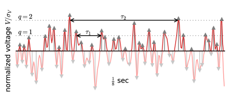
Rysunek 1: Schematic illustration of inter–pulse intervals. Shown are the normalized data (red) together with the related point process (gray) for $\nicefrac{{1}}{{8}}$ second of total 10 seconds of recording. The black line illustrates the baseline signal, here at $q=0$. Triangles directed upwards (downwards) mark the positive maxima (negative minima). Arrows depict exemplary IPIs $\tau_{1}$ and $\tau_{2}$ for the respective threshold values $q=1$ (bottom) and $q=2$ (top).

The process consists of positive maxima (negative minima) created by the electrical activities of MU, cf. Fig. 1. In the following we limit to the description of the ’upper’ part of the signal where $V\geq 0$. Exactly the same procedure can be adopted for ’lower’ negative fraction, thus gives the improvement of the statistics. The maxima above the baseline were used in the construction of the point process. As each maximum is replaced by the point of the same height as the analogous maximum and all other values of the signal are set to zero the resulting time train of discrete spikes constitute a point process which can be described by the random intervals between the points. The archetype of the point process is well known Poisson process (or Poisson point field) which has the property that each point is stochastically independent of all the other points in the process [20]. As such, the distribution of the intervals between the consecutive points is known to be exponential. Despite being a limiting case of Bernoulli trials, the process was shown to have numerous applications in distant branches of science, including astronomy [21], biology [22], image processing [23], finance markets [24], or even for classical [25] and quantum [26] dynamical systems, to name but a few.

As we are interested in statistical properties of the signal at all possible scales of volatilities, small, intermediate and large, the range of thresholds $q$ were set from 0 to the maximum possible value of rescaled voltage, above which at least $10$ maxima were found. This will allow for the description of the properties of the whole signal, regardless the scale. The maximum value of the threshold would differ for each channel, depth and stage of treatment for every analyzed patient. Nevertheless, the threshold was found never to exceed $q=10$.

Data acquisition

Signals were obtained with use of reusable anal probe developed at Laboratory of Engineering of Neuromuscular System and Motor Rehabilitation of Politecnico di Torino in collaboration with the company OT-Bioelettronica. The probe thickness is 14 mm and it has 3 rings of 16 silver bar electrodes each. Electrodes are placed parallel to the long axis of the probe and have dimensions of $9\times 1$ mm. There is an 8 millimeter distance between each of the rings hence they enable recordings at 3 different levels of anal canal. Probe was positioned in a way that first ring would be placed starting from the anal verge, second would start at 18 mm and third one at 35 mm. The sampling frequency was 2048 Hz, which for the 10 seconds of the measurement gave 20480 data points. The probe was connected to the standard PC over 12 bit NI DAQ MIO16 E-10 transducer (National Instruments, USA). Low and high pass filters were used at 10 and 500 Hz respectively which gave a bandwidth equal to 3 dB. The monopolar signals were obtained by differential acquisition of the signals detected from each pair of the electrodes of the probe with respect to a reference strip connected to the patient wrist [27]. For the time of the acquisition patients were positioned in left lateral decubitus position. Measurement were conducted in a constant pattern: 1 minute relaxation, three 10 sec long recordings at rest for each depth, 1 minute relaxation and then three 10 sec long recordings at maximum voluntary contraction (MVC) for each depth with additional 1 minute breaks in between. The whole process was repeated twice, which gave 12 recordings for a patient for each time point. The recordings were conducted at four time points of treatment - before the surgical procedure ($D_{1}$) and 1 month ($D_{2}$), 6 months ($D_{3}$) and 1 year ($D_{4}$) after the surgery.

Patients

The study included 16 subjects, 5 female, age range 46 to 71 (average 56 years) and 11 male, age range 40 to 85 (average 63,6 years), diagnosed with rectal cancer and qualified for surgery. Based on localization of rectal cancer patients underwent either Low Anterior Resection (LAR) - 9 patients, Anterior Resection (AR) - 6 patients or proctocolectomy (PC) - 1 patient. The detailed information about the surgery of the rectal cancer and the role of sEMG for the patient diagnosis can be found in [28, 29].

Analysis

The statistical properties of the inter–pulse intervals (IPIs) between consecutive maxima (see $\tau_{1}$ and $\tau_{2}$ in Fig 1) of the sEMG signals is the subject of this work. Thresholds at which the intervals were calculated were determined in the logarithmic manner from $0$ (effectively taken all of the maxima) up to the value where at least $10$ IPIs were evident. Keep in mind that thresholds were also scaled with the standard deviations $\sigma_{V}$ complementary to the signals.

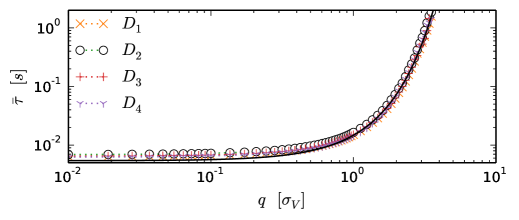
Rysunek 2: The generic characteristics of the average IPI time $\bar{\tau}$ versus the threshold magnitude $q$ presented for all stages $D_{1}$ – $D_{4}$ of treatment. Please note almost identical relation for all stages. Maximal threshold value for which at least $10$ IPIs were found does not reach $q=4$. The black line presenting fitted exponent is shown to lead the eye.

The typical dependence of the mean IPI time $\bar{\tau}$ on threshold $q$ is presented in Fig 2 for the selected patient and for all stages $D_{1}$ – $D_{4}$ of treatment. As expected it is the monotonic function of the threshold value with the evident exponential growth. The presented behavior seems to be the typical situation for the data registered for all patients. It means, that the knowledge on the average IPI will not help to classify the stage of treatment. Maximal threshold values for which at least $10$ IPIs were found do not reach $q=4$ for most examined cases. For small values of the threshold the mixed statistical properties of MUAPs, the background noise, failed initiations of MUAPs as well as refractory periods of MUAPs or satellite waves are all taken into consideration. For intermediate levels of $q$ one can expect only MUAPs and satellite waves to contribute to the effective, above the threshold train of pulses. For large thresholds, $q>2$, the average waiting times between consecutive maxima grows by the order of magnitude therefore are likely to portray only the properties of MUAPs.

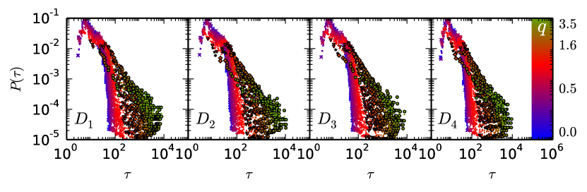
Rysunek 3: Probability distribution function $P(\tau)$ presented for several threshold values $q$. Computed PDFs cannot be represented by one specific function. The PDF for the threshold level are indicated by the colour – see colour bar on the right.

Next, we study the behavior of the probability distribution function (PDF) and it’s dependence on the threshold value $q$. For different thresholds PDFs are different cf. Fig 3 and cannot be represent by the same function. In particular they cannot be described by the Poisson distribution $\propto\exp(-\tau)$ as for the uncorrelated data. This in turn allows to draw a conclusion of existing correlations hidden in the acquired data. To shed some more light on the actual influence of the threshold value the scaled PDFs $P(\tau)\bar{\tau}$ as a function of the scaled inter–pulse interval $\tau/\bar{\tau}$ is presented in Fig 4. Again the different colors, blue – purple – red – orange – green, reflect the growing threshold dependence, from $q=0$ up to $q\simeq 4$. Different symbols group the IPIs for different values of the average IPI $\bar{\tau}$, with $\times$ being equivalent to average time shorter than $0.01$ sec and $\circ$ longer than $0.1$ sec. As one can notice the scaled PDF $P(\tau)\bar{\tau}$ dependence on scaled IPI is found to be different both for different average times (marked by symbols) and thresholds (marked by colors). Keep in mind an exponential correspondence between $\bar{\tau}$ and $q$, cf. Fig 2.

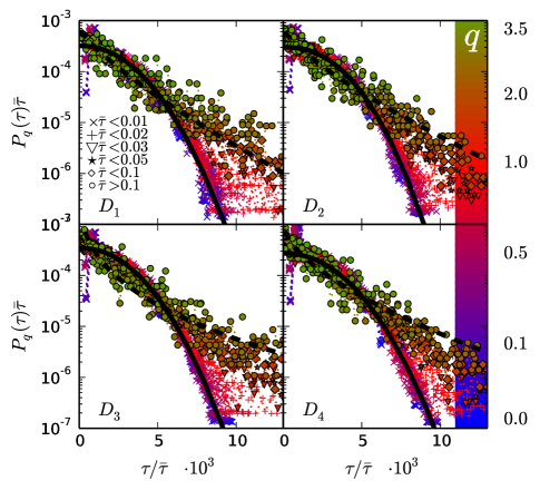
Rysunek 4: Probability distribution function scaled with the average IPI time $\bar{\tau}P(\tau)$ versus scaled IPI time $\tau/\bar{\tau}$. Different symbols were used in order to provide the visual guidance for different average IPIs – see legend in top right panel ($D_{1}$). For all the stages $D_{1}-D_{4}$ one can reveal the stretched–exponential function (2) with the threshold $q$ dependent parameters. Again the PDFs for the different threshold $q$ level are indicated by the colour – see colour bar on the right.

In spite of the visual differences of the scaled probability distribution function

$$P_{q}(t)=\frac{1}{\bar{\tau}}f_{q}\left(\frac{t}{\bar{\tau}}\right)$$ (1)

for different average IPIs or thresholds, equivalently, the analysis is consistent with the possibility that the data can be characterized by the stretched exponential function

$$f_{q}(x)\propto\exp(-b_{q}x^{\beta_{q}})$$ (2)

where all the parameters $\{b_{q},\beta_{q}\}$ are threshold dependent.

Correlation between records

For uncorrelated records one expects the data to follow the exponential Poisson distribution. Here we claim, that the analyzed IPIs do possess the correlations. To test this expectations and prove the long-term memory we shuffle the inter–pulse intervals $\tau$ and investigate the resultant PDFs. The shuffled data indeed follow the Poisson distribution, see Fig 5. This form of the PDF for the shuffled IPIs suggest that the stretched exponential form of the distribution function for the original IPI emerges from the correlations.

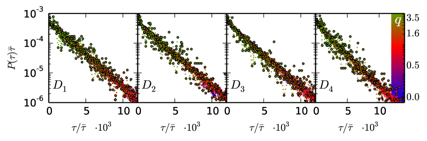
Rysunek 5: Probability distribution function for the shuffled IPIs. For all the stages $D_{1}$–$D_{4}$ one can reveal the exponential Poisson-like distribution $\log[P_{q}\bar{\tau}]=-\tau/\bar{\tau}$, seen as a linear function on the semi-logarithmic plot.

The closer look at the inter–pulse intervals trains of original and shuffled data are rather similar, cf. Fig 6. There are also no visible clustering, or any other indications of memory – the events look simply random. If the distribution (1) suppose to fully characterize the underlying data, the subsequent IPIs should not be dependent on each other, and only be chosen randomly from the distribution (1). In turn, the obtained PDF would fully characterize the data.

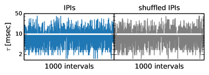
Rysunek 6: Typical train of the analyzed inter–pulse intervals. On the l.h.s. the original train of the $D_{1}$ stage of one of the patients is presented for the average inter–pulse interval $\tau=0.01$ msec. On the r.h.s. shuffled data is shown.

To test the possible effects of memory among the intervals we study the conditional probability distribution function $P_{q}(\tau|\tau_{0})$ of the intervals $\tau$ which directly follow the interval $\tau_{0}$. In order to do so first we sort the IPIs in the ascending order. Next we split just sorted intervals into four equinumerous subsets $\{S_{1},S_{2},S_{3},S_{4}\}$. The shortest intervals will fall into the first set $S_{1}$ while the longest intervals will be stored in the last one $S_{4}$. The results shown in Fig 7 demonstrate the same exponential behavior of the conditional PDF for any threshold $q$ regardless the set the $\tau_{0}$ was taken from. In Fig 7 one can find plots of the conditional PDF $P_{q}(\tau|\tau_{0})$ scaled with the average interval $\bar{\tau}$ as a function of the scaled IPI $\tau/\bar{\tau}$.

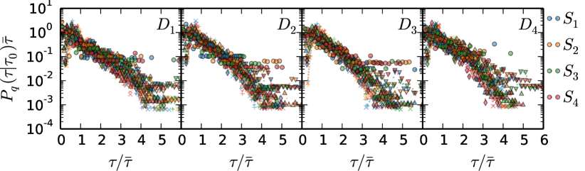
Rysunek 7: Conditional probability distribution function for IPIs. For all the stages $D_{1}$–$D_{4}$ one can reveal the exponential Poisson-like distribution $\log[P_{q}(\tau|\tau_{0})\bar{\tau}]=-\tau/\bar{\tau}$, seen as a linear function on the semi-logarithmic plot.

Four different colors blue, orange, green and red were used to indicate the correspondent subset $\{S_{1},S_{2},S_{3},S_{4}\}$ respectively. On top of that one can track the behavior of conditional PDF for different threshold values $q$. There is a striking correspondence for all subsets and thresholds. It means that there is no memory effects between the consecutive intervals, also for the case of high thresholds. This in turn indicates that the anterior MUAP has no influence on the posterior one.

Results and Discussion

Lack of the memory effects in the IPI trains as well as Poisson like exponential shape of the PDFs for shuffled data let us state the hypothesis that the threshold dependent PDFs for the IPIs (1) fully describe the behavior of the inter–pulse intervals of surface electromyography signals acquired from patients with colorectal cancer. Now we take a look at the actual shape of the stretched exponential $f_{q}\propto\exp(-b_{q}x^{\beta_{q}})$ (2) .

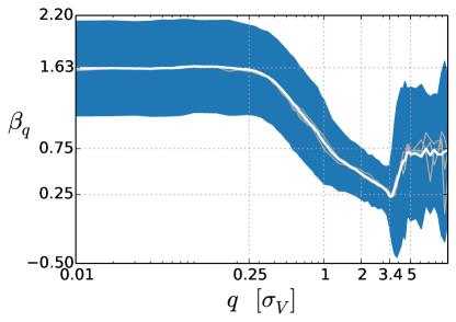
Rysunek 8: Average value of the shape parameter $\beta_{q}$ versus the threshold level $q$. shown at all four stages of treatment. The white line represent the global average calculated for all possible cases $D_{1}$ – $D_{4}$ and at both states MVC and at rest. Barely visible gray lines which represent separate states $D_{1}$ – $D_{4}$ shadow the global average. The dark blue band represents the standard deviation $\sigma_{\beta_{q}}$.

The threshold dependence of the shape parameter $\beta_{q}$ is presented in the Fig 8. For all of the analyzed data the $q$ dependence can be characterised as a non–monotonic function. As expected for relatively low values of threshold $q<0.25\sigma_{V}$ i.e. for the situation of all the possible pulses analyzed the average value of the shape parameter is constant and close to $\beta_{q}\simeq 1.62$. Next it decreases with increasing $q$ reaching a value of around $\beta_{q}\simeq 0.25$ for the threshold $q\simeq 3.4\sigma_{V}$. From this value onwards it increases and saturates close to $\beta_{q}\simeq 0.75$ for thresholds higher than $5\sigma_{V}$. The last part corresponds to the highest pulses which can be treated as MUAPS. This behavior is not dependent on the stage of treatment $D_{1}$–$D_{2}$. In the Fig 8 one can find gray lines which correspond to the consecutive stages and shadow the average value. Up to the threshold values close to $5\sigma_{V}$ these are rather indistinguishable from each other and from the average value of the shape parameter. Above this value the number of events drops drastically, thus the resulting statistics is weaker and the discrepancies between stages and the average values are found. Nevertheless the tendency is similar and all the curves fluctuate around the same average value.

From the above analysis it follows that the statistics of the inter–pulse intervals of the particular stages of colorectal cancer treatment are similar. The scaled probability distribution functions $\bar{\tau}P_{q}(\tau)$ of the rescaled IPIs $\tau/\bar{\tau}$ exhibit stretched–exponential behavior with the threshold (average IPI) dependent shape $\beta_{q}$ and scale $b_{q}$ parameters. The actual PDF seems to be the sufficient characteristics for the description of the process. Existing long time correlations purely comes from the distribution - the shuffled data show clean exponential nature. Clustering events were also not detected for all of the stages.

Based on our data we can conclude that analyzed parameters are not influenced by multimodal treatment of rectal cancer hence the probability that aforementioned treatment affects inter–pulse intervals between the extrema of an electrical activity of External Anal Sphincter is minimal.

- [1] S. Bernard and W. Christopher, “World cancer report 2014,” tech. rep., World Health Organization, 2014.
- [2] F. Bray, A. Jemal, N. Grey, J. Ferlay, and D. Forman, “Global cancer transitions according to the human development index (2008–2030): a population-based study,” The lancet oncology, vol. 13, no. 8, pp. 790–801, 2012.
- [3] J. Ferlay, I. Soerjomataram, R. Dikshit, S. Eser, C. Mathers, M. Rebelo, D. M. Parkin, D. Forman, and F. Bray, “Cancer incidence and mortality worldwide: sources, methods and major patterns in globocan 2012,” International journal of cancer, vol. 136, no. 5, pp. E359–E386, 2015.
- [4] H. Ikeuchi, M. Kusunoki, Y. Shoji, T. Yamamur, and J. Utsunomiya, “Clinico-physiological results after sphincter-saving resection for rectal carcinoma,” International journal of colorectal disease, vol. 11, no. 4, pp. 172–176, 1996.
- [5] G. Batignani, I. Monaci, F. Ficari, and F. Tonelli, “What affects continence after anterior resection of the rectum?,” Diseases of the colon & rectum, vol. 34, no. 4, pp. 329–335, 1991.
- [6] H. Suzuki, K. Matsumoto, S. Amano, M. Fujioka, and M. Honzumi, “Anorectal pressure and rectal compliance after low anterior resection,” British Journal of Surgery, vol. 67, no. 9, pp. 655–657, 1980.
- [7] W. G. Lewis, I. G. Martin, M. E. Williamson, B. M. Stephenson, P. J. Holdsworth, P. J. Finan, and D. Johnston, “Why do some patients experience poor functional results after anterior resection of the rectum for carcinoma?,” Diseases of the colon & rectum, vol. 38, no. 3, pp. 259–263, 1995.
- [8] G. Rao, P. Drew, P. Lee, J. Monson, and G. Duthie, “Anterior resection syndrome is secondary to sympathetic denervation,” International journal of colorectal disease, vol. 11, no. 5, pp. 250–258, 1996.
- [9] J. Hill, G. Hosker, and E. Kiff, “Pudendal nerve terminal motor latency measurements: what they do and do not tell us,” British journal of surgery, vol. 89, no. 10, pp. 1268–1269, 2002.
- [10] W. Floyd and E. Walls, “Electromyography of the sphincter ani externus in man,” The Journal of physiology, vol. 122, no. 3, p. 599, 1953.
- [11] J. R. Daube and D. I. Rubin, “Needle electromyography,” Muscle & nerve, vol. 39, no. 2, pp. 244–270, 2009.
- [12] J. M. Remes-Troche and S. S. Rao, “Neurophysiological testing in anorectal disorders,” Expert review of gastroenterology & hepatology, vol. 2, no. 3, pp. 323–335, 2008.
- [13] C. J. De Luca, “The use of surface electromyography in biomechanics,” Journal of applied biomechanics, vol. 13, no. 2, pp. 135–163, 1997.
- [14] R. Merletti, A. Bottin, C. Cescon, D. Farina, M. Gazzoni, S. Martina, L. Mesin, M. Pozzo, A. Rainoldi, and P. Enck, “Multichannel surface emg for the non-invasive assessment of the anal sphincter muscle,” Digestion, vol. 69, no. 2, pp. 112–122, 2004.
- [15] C. Cescon, L. Mesin, M. Nowakowski, and R. Merletti, “Geometry assessment of anal sphincter muscle based on monopolar multichannel surface emg signals,” Journal of Electromyography and Kinesiology, vol. 21, no. 2, pp. 394–401, 2011.
- [16] I. Rodríguez-Carreño, A. Malanda-Trigueros, and L. Gila-Useros, Motor unit action potential duration: Measurement and significance. INTECH Open Access Publisher, 2012.
- [17] D. Winter, A. Fuglevand, and S. Archer, “Crosstalk in surface electromyography: theoretical and practical estimates,” Journal of Electromyography and Kinesiology, vol. 4, no. 1, pp. 15–26, 1994.
- [18] P. Konrad, “The abc of emg,” A practical introduction to kinesiological electromyography, vol. 1, pp. 30–35, 2005.
- [19] C. J. De Luca and W. J. Forrest, “Some properties of motor unit action potential trains recorded during constant force isometric contractions in man,” Kybernetik, vol. 12, no. 3, pp. 160–168, 1973.
- [20] D. J. Daley and D. Vere-Jones, An introduction to the theory of point processes. vol. I. , Elementary theory and methods. Probability and its applications, New York, Berlin, Paris: Springer, 2003.
- [21] G. J. Babu and E. D. Feigelson, “Spatial point processes in astronomy,” Journal of statistical planning and inference, vol. 50, no. 3, pp. 311–326, 1996.
- [22] H. G. Othmer, S. R. Dunbar, and W. Alt, “Models of dispersal in biological systems,” Journal of mathematical biology, vol. 26, no. 3, pp. 263–298, 1988.
- [23] M. Bertero, P. Boccacci, G. Desiderà, and G. Vicidomini, “Image deblurring with poisson data: from cells to galaxies,” Inverse Problems, vol. 25, no. 12, p. 123006, 2009.
- [24] K. Yamasaki, L. Muchnik, S. Havlin, A. Bunde, and H. E. Stanley, “Scaling and memory in volatility return intervals in financial markets,” Proceedings of the National Academy of Sciences of the United States of America, vol. 102, no. 26, pp. 9424–9428, 2005.
- [25] J. Spiechowicz, J. Łuczka, and P. Hänggi, “Absolute negative mobility induced by white poissonian noise,” Journal of Statistical Mechanics: Theory and Experiment, vol. 2013, no. 02, p. P02044, 2013.
- [26] J. Luczka and M. Niemiec, “A master equation for quantum systems driven by poisson white noise,” Journal of Physics A: Mathematical and General, vol. 24, no. 17, p. L1021, 1991.
- [27] C. Cescon, L. Mesin, M. Nowakowski, and R. Merletti, “Geometry assessment of anal sphincter muscle based on monopolar multichannel surface EMG signals,” J Electromyogr Kinesiol, vol. 21, pp. 394–401, Apr 2011.
- [28] G. G. Delaini, M. Scaglia, G. Colucci, and L. Hultén, “Functional results of sphincter-preserving operations for rectal cancer,” in Rectal Cancer, pp. 147–155, Springer, 2005.
- [29] A. López, B. Y. Nilsson, A. Mellgren, J. Zetterström, and B. Holmström, “Electromyography of the external anal sphincter,” Diseases of the colon & rectum, vol. 42, no. 4, pp. 482–485, 1999.