Sequencing of semiflexible polymers of varying bending rigidity using patterned pores

Abstract

We study the translocation of a semiflexible polymer through extended pores with patterned stickiness, using Langevin dynamics simulations. We find that the consequence of pore patterning on the translocation time dynamics is dramatic and depends strongly on the interplay of polymer stiffness and pore-polymer interactions. For heterogeneous polymers with periodically varying stiffness along their lengths, we find that variation of the block size of the sequences and the orientation, results in large variations in the translocation time distributions. We show how this fact may be utilized to develop an effective sequencing strategy. This strategy involving multiple pores with patterned surface energetics, can predict heteropolymer sequences having different bending rigidity to a high degree of accuracy.

I Introduction

Polymer translocation is relevant to various biological processes such as the passage of mRNA through nuclear pores after transcription, horizontal gene transfer in bacterial conjugation and viral injection of DNA into host cells Frank2010 ; Salman2001 . In the last two decades, polymer translocation has attracted considerable attention both experimentally Service2006 ; Lagerqvist2006 ; Branton2008 ; Shendure2008 ; Schloss2008 ; Persson2010 ; Zwolak2008 ; Min2011 ; Kasianowicz1996 ; Braha1997 ; Akeson1999 ; Meller2000 ; Meller2001 ; Deamer2002 ; Meller2003 ; Maglia2008 and theoretically lubensky ; luo2006jcp ; muthukumar ; Polson2013 ; matysiak ; luo2007prl ; luo2008pre ; luo2008prl ; luo2007jcp ; mirigian2012 ; gauthier ; luan ; nikoubashman ; sung ; Muthukumar1999 ; muthukumar2001 ; kantor2001 ; muthukumar2003 ; metzler ; slonkina ; kantor2004 ; milchev2004 ; gerland ; gopinathan ; wong ; milchev2011 ; abdolvahab2011 ; Cohen2011 ; Sakaue2007 ; Sakaue2010 ; Rowghanian2011 ; Saito2011 ; Dubbeldam2012 ; Ikonen2012 ; Ikonenjcp2012 ; Sarabadani2014 ; Sarabadani2017 ; Lehtola2009 ; Haan2010 ; Bhattacharya2013 ; Adhikari2013 ; Adhikari2015 ; Cohen2012 ; Cohen2013 ; Katkar2014 due to its potential technological applications, such as controlled drug delivery, gene therapy, and rapid DNA sequencing Branton2008 . Experiments have demonstrated that single stranded DNA and RNA molecules can be electrophoretically driven through biological and synthetic nanopores Kasianowicz1996 ; Deamer2002 . During polymer translocation, the ion current flowing through the channel gets blocked, indicating the presence of the polymer inside the pore. The current blockade readout which could potentially serve as a signature of the sequence of the polymer segment inside the pore, opens up the possibilities of efficient sequencing methods Kasianowicz1996 .

Most biopolymers and proteins are semiflexible, implying that the energy cost to bend the polymer exceeds the entropic propensity to form a random coil configuration Dhar2002 ; Frey1996 . The bending stiffness of semiflexible polymers is quantified by the persistence length, $\ell_{p}$, the length over which the polymer appears rigid. Experimental studies indicate that sequence dependent bending rigidity is important for DNA-protein interaction and nucleosome positioning Widom2001 ; Travers2004 . Such a dependence is confirmed from cyclization studies of short DNA fragments, which allows accurate measurement of persistence length Geggier2010 . Therefore, sequencing techniques based on polymer translocation, which could correctly sense this variation, necessitates the study of heteropolymers with varying bending stiffness as they pass through a nanopore. Other examples of polymers with varying bending rigidity includes partially melted DNA and proteins which exhibit stiff and flexible segments along the polymer backbone  Branden1998 ; Lee2001 ; Stellwagen2003 ; Kowalczyk2010 .

The complex and subtle nature of the translocation process is apparent in the different theoretical estimates of the exponent $\delta$ reported in the scaling of the mean translocation time $\langle\tau\rangle$ with the chain length ${\cal L}$, $\langle\tau\rangle\sim{\cal L}^{\delta}$. Sung and Park sung and Muthukumar Muthukumar1999 ; muthukumar2001 considered the translocation process as a one dimensional barrier crossing problem with the assumption that the translocation time is long enough to ensure equilibration of the polymer conformations at every stage of the process. There have been a plethora of later studies predicting different exponents using arguments like dynamical scaling kantor2001 ; kantor2004 , mass and energy conservations Rowghanian2011 and tension propagation (TP) along the length of the polymer Sakaue2007 ; Sakaue2010 ; Saito2011 . TP theory, introduced originally by Sakaue Sakaue2007 for an infinite chain and subsequently modified by Ikonen et al. Ikonen2012 ; Ikonenjcp2012 and Dubbeldam et al. Dubbeldam2012 to finite chains have proved to be successful in explaining the non-equilibrium facets of driven translocation. In TP theory, the translocation process is described in terms of a single variable, the monomer index, $s$, at the pore. The part of the translocating polymer on the cis-side is divided into two distinct domains. The external driving force that acts inside the pore, pulls the monomers nearer to the pore and sets them in motion. The remaining monomers that are farther away from the pore, do not experience the pull and on average remain at rest. As the polymer gets sucked inside, more and more monomers on the cis side start responding to the force, with a tension front separating the two domains propagating along the length of the polymer. At time $t$, the drag, experienced by a monomer inside the pore, can be written as the sum of the friction due to the length of the chain in the cis side up to which the tension has propagated, the trans side segment and the pore friction. It is then easy to see that this drag increases as the tension front propagates and more number of monomers on the cis side get involved. This increase in the effective friction is manifested in the mean waiting times, $w(s)$, defined as the amount of time a monomer $s$ spends on average inside the pore. The results from simulation studies of a flexible homopolymer, passing through a pore of unit length, shows an initial increase with $s$, implying that the subsequent monomers spend more time inside the pore. This continues until the drag becomes maximum when the tension front reaches the last monomer. The time at which this happens is called the tension propagation time ($t_{tp}$). At $t_{tp}$, a maximum number of monomers at the cis-side participate in the translocation process and the monomer $s$, which is inside the pore at that instant, has maximum waiting time $w(s)$. For $t>t_{tp}$, the system enters the tail retraction stage, where the monomers on the cis side starts decreasing, and therefore the drag decreases, and so does the waiting time $w(s)$.

The TP theory Ikonen2012 ; Ikonenjcp2012 correctly accounts for the role of pore friction and thermal fluctuations due to the solvent and their effects on the scaling exponent. Further, it explains various values of the exponent observed in previous studies, thereby providing a unifying picture of polymer translocation. The theory was recently modified with a constant monomer iso-flux approximation by Sarabadani et al. Sarabadani2014 ; Sarabadani2017 , which leads to a self consistent theory for polymer translocation with effective pore friction as the only free parameter. Bhattacharya and others Bhattacharya2013 ; Adhikari2013 ; Adhikari2015 ; Haan2010 used TP theory to explain the dependence of translocation times on the stiffness of a semiflexible polymer. It was found Adhikari2013 ; Adhikari2015 that the peak of the waiting time shifts towards lower $s$ indicating that $t_{tp}$ decreases: i.e., the tension propagates faster along the backbone, as the stiffness of the polymer increases.

A large number of the results discussed above were for pores of small size, where the pore polymer interactions are negligible. However, experiments involve pores of finite length, where pore-polymer interactions play a dominant role. Solid state nanopores with tailored surface properties Storm2003 ; Kim2006 make it possible to regulate the interactions of the polymer with the pore as well as reducing noise Ohshiro2006 ; Iqbal2007 ; Wanunu2007 ; Chen2004 ; Tabard2007 . Luo et. al. luo2007prl ; luo2008pre ; luo2008prl showed that the mean translocation time of a polymer across an attractive channel increases with the strength of attraction. This suggests a possibility to separate polymers with varying interactions with the pore. Furthermore, translocation dynamics of a heterogenous polymer through an extended pore show a strong dependence on the sequence. The heterogeneity has been introduced in a variety of ways. Luo et. al. luo2007jcp considered heteropolymers consisting of two types of monomers which are distinguished by the driving force they experience inside the pore. The residence time of each bead inside the pore was found to be a strong function of the sequence. Mirigian et. al. mirigian2012 considered polymers with differing frictional interaction with the pore and charge. The mean translocation time of the multiblock polymers depends on the fraction as well as the arrangement of the blocks. At a certain optimum length of the charged block, the mean translocation rate is the slowest. Recent theoretical studies Cohen2012 ; Cohen2013 ; Katkar2014 considered channels with varying pore-polymer interactions along its length. The translocation time distributions showed significant variations across the differently decorated channels. Katkar and Muthukumar Katkar2014 showed that translocation time across a nanopore of alternate charged and uncharged sections, depends non-monotonically on the length of the charged section. In the studies by Cohen et. al. Cohen2012 ; Cohen2013 , it was shown that the statistical fluctuations in the translocation time could be utilised for efficient sequencing of heteropolymers, by suitably engineering pore-polymer interactions and combining readouts from multiple pores.

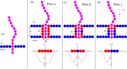
Figure 1: Schematic diagram of a semiflexible polymer of stiffness $\lambda$ translocating from the cis to the trans side through (a) Pore of unit length ($L=\sigma$) and three extended patterned pores (b) Pore $\alpha$ (c) Pore $\beta$, and (d) Pore $\gamma$ of length $L$ and width $W$. A driving force ${\boldsymbol{F}}_{\textrm{ext}}=F\hat{\boldsymbol{x}}$ acts on every monomer inside the pore. The potential energy of a polymer bead along the pore axis due to pore beads on either side, for various pore types is also shown.

In this paper, we propose a sequencing strategy to accurately detect heteropolymers with sequence dependent bending rigidity through extended patterned pores. Driving a homogeneous semiflexible polymer through extended pores with different patterned stickiness, we establish the interplay of pore-polymer interactions and polymer rigidity in determining translocation time statistics. We find that a stiffer polymer takes more time to translocate through patterned pores, similar to that observed for pores of unit length Adhikari2013 . However, the mean waiting times of monomers near the pore entrance and exit vary greatly depending on the pore patterns, a feature distinct for extended patterned pores. We utilize these dependencies to test the possibility of detecting heteropolymers consisting of alternate blocks of stiff and flexible segments, by passing them through multiple pores. We show that driven translocation of heteropolymers with varying bending stiffness through extended pores, when coupled to pore patterning, can lead to efficient sequence detection.

The paper is organized as follows: In Sec. II, we define our model and the various pore patterns studied in this paper. In Sec. III, we discuss results for the driven translocation of semiflexible polymer of homogeneous stiffness through extended patterned pores. The results for the driven translocation of semiflexible polymer consisting of alternate blocks of stiff and flexible segments and the sequencing method are discussed in Sec. IV. Finally, we summarize our results in Sec. V.

II Model and Simulation Details

Homopolymer model. The polymer is modeled as a self-avoiding semiflexible polymer by using beads and springs in two dimensions (Fig. 1). Semiflexibility is introduced by the bending energy term

$$U_{\textrm{bend}}=\frac{\kappa_{b}}{2\sigma}\sum_{i=1}^{N-2}[{\bf t}_{i+1}-{\bf t}_{i}]^{2},$$ (1)

where $\kappa_{b}$ is the bending rigidity of the polymer, $\sigma$ is the equilibrium bond length and ${\bf t}_{i}=[{\bf r}_{i+1}-{\bf r}_{i}]/b_{i}$ is the local tangent. Here, $b_{i}=|{\bf r}_{i+1}-{\bf r}_{i}|$ is the instantaneous bond length. $\kappa_{b}$ represents the stiffness of the polymer, and in two dimensions it is related to the persistence length as $\kappa_{b}/k_{B}T=\ell_{p}/2$, where $k_{B}$ is the Boltzmann’s constant and $T$ is the temperature.

The beads of the polymer experience an excluded volume interaction modeled by the Weeks-Chandler-Andersen (WCA) potential of the form

$$U_{\textrm{bead}}(r)=\begin{cases}4\epsilon\left[\left(\frac{\sigma}{r}\right)^{12}-\left(\frac{\sigma}{r}\right)^{6}\right]+\epsilon&\text{for}\ r\leq r_{min}\cr 0&\text{for}\ r>r_{min},\end{cases}$$ (2)

where, $\epsilon$ is the strength of the potential. The cut-off distance, $r_{min}=2^{1/6}\sigma$, is set at the minimum of the potential. Consecutive monomers in the chain interact via the finite extension nonlinear elastic (FENE) potential of the form

$$U_{\textrm{bond}}(r)=-\frac{1}{2}kR^{2}\ln\left(1-\frac{r^{2}}{R^{2}}\right),$$ (3)

where $k$ is the spring constant and $R$ is the maximum allowed separation between consecutive monomers of the chain. The length of the polymer is given by $N\sigma$, where $N$ is the number of beads.

Heteropolymer model. A heteropolymer is modelled similarly by using beads and springs with the polymer segment representing $n$ monomers each of stiff ($S$) and flexible ($F$) beads arranged in symmetric blocks $S_{n}F_{n}$. A schematic diagram of such a polymer with $n=4$ is shown in Fig. 2(a). As an example, for a polymer with $N=128$, the minimum value of $n=1$ is for $(S_{1}F_{1})_{64}$, i.e., 64 repeat units of $S_{1}F_{1}$, and the maximum value of $n=N/2=64$ is for a single unit of $S_{64}F_{64}$. For a heteropolymer, it makes a difference whether a flexible or a stiff end enters the pore first (Figs. 2(b), 2(c), 2(d)).

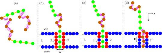
Figure 2: (a) Schematic diagram of a polymer with alternate blocks of stiff (S) and flexible (F) segments $S_{n}F_{n}$ each having $n=4$ bonds. The stiff (S) and flexible (F) bonds are shown by straight and zig-zag lines, respectively. (b) and (c) Polymer $S_{4}F_{4}$ translocating through Pores $\alpha$ and $\beta$, respectively, with the stiff end entering the pore first. (d) Polymer $F_{4}S_{4}$ translocating trough Pore $\gamma$ with the flexible end entering the pore first.

Pore model. The pore and the wall are made from stationary monomers separated by a distance of $\sigma$ from each other. The pore is made up of two rows of monomers symmetric about the $x$-axis. The length of the pore is taken to be $L$ with a diameter $W$ (see Fig. 1).

We choose extended pores of length $L=5\sigma$ with three different pore patterns :

1. Pore $\alpha$ is an attractive pore. All the monomers of the pore interact with the polymer by the LJ potential :

   $$U_{\textrm{pore}}(r)=\begin{cases}4\epsilon_{\textrm{pore}}\left[\left(\frac{\sigma}{r}\right)^{12}-\left(\frac{\sigma}{r}\right)^{6}\right]&\text{for}\ r\leq r_{c}\cr 0&\text{for}\ r>r_{c},\end{cases}$$ (4)

   where $\epsilon_{\textrm{pore}}$ denotes the potential depth and $r_{c}=2.5\sigma$ is the cut-off distance.

2. Pore $\beta$ has an attractive entrance and exit. The first two and the last two monomers of the pore interact with the polymer by the LJ potential, and the middle monomer by WCA potential as in the pore of unit length.

3. Pore $\gamma$ has an attractive entrance and repulsive exit. The first two monomers of the pore interact with the polymer by the LJ potential and the last two monomers of the pore by WCA potential as above.

The interaction between the wall beads and of the polymer ($U_{\textrm{wall}}$), is the same as the intramonomer interaction ($U_{\textrm{bead}}$).

To facilitate transfer from the cis to the trans side of the pore, the polymer experiences a driving force, ${\boldsymbol{F}}_{\textrm{ext}}=F\hat{\boldsymbol{x}}$ directed along the pore axis with magnitude $F$, which acts on every polymer bead inside the pore. This mimics the electrophoretic driving of biopolymers through nanopores. Due to the larger entropic cost involved in confining the polymer in extended pores, the pore entrance in such cases are chosen to be attractive to initiate the translocation successfully. A schematic diagram of semiflexible polymers translocating from the cis to the trans side through the pore of unit length and pores $\alpha$, $\beta$, and $\gamma$ are shown in Fig. 1(b)-(d), respectively.

To integrate the equation of motion for the monomers of the chain we use Langevin dynamics algorithm with velocity Verlet update. The equation of motion for a monomer is given by

$$m\ddot{\boldsymbol{r}}_{i}=-{\boldsymbol{\nabla}}U_{i}+{\boldsymbol{F}}_{ext}-\zeta{\boldsymbol{v}}_{i}+{\boldsymbol{\eta}}_{i},$$ (5)

where $m$ is the monomer mass,

$$U_{i}=U_{\textrm{bend}}+U_{\textrm{bond}}+U_{\textrm{bead}}+U_{\textrm{wall}}+U_{\textrm{pore}},$$

is the total potential experienced by a monomer, $\zeta$ is the friction coefficient, ${\boldsymbol{v}}_{i}$ is the monomer velocity, and ${\boldsymbol{\eta}}_{i}$ is the random force with mean $\langle\eta(t)\rangle=0$ satisfying the fluctuation-dissipation theorem $\langle{\eta}_{i}(t){\eta}_{j}(t^{\prime})\rangle=2\zeta k_{B}T\delta_{ij}\delta(t-t^{\prime})$.

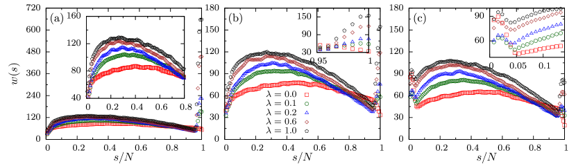
Figure 3: Mean waiting times $w(s)$ for monomers of a semiflexible polymer of various stiffness $\lambda$ for (a) Pore $\alpha$, (b) Pore $\beta$, and (c) Pore $\gamma$. The inset in (a) represents $w(s)$ for Pore $\alpha$ excluding the end monomers. Inset in (b) shows the end monomers region for Pore $\beta$ while inset in (c) shows the behavior for the initial monomers entering the pore for Pore $\gamma$. Note that error bars are smaller than the point size and are not shown here.

The unit of energy, length and mass are set by the familiar $LJ$ units $\epsilon$, $\sigma$ and $m$ respectively. This sets the unit of time as $\sqrt{m\sigma^{2}/\epsilon}$. In these units, we choose $N=128$, $L=5$, $W=2.25$, $\epsilon_{\textrm{pore}}=1.2$ (homopolymer), $r_{c}=2.5$, $\zeta=0.7$, $k=30$, $R=1.5$ and $k_{B}T=1.2$, in our simulations. These parameters are in accordance with earlier Langevin dynamics simulations for polymer translocation luo2007prl ; luo2008prl ; Cohen2011 ; Cohen2012 ; Cohen2013 . The choice of pore width ensures single-file translocation of the polymer and avoids the formation of hairpin configurations inside the pore. The stiffness of the semiflexible polymer is characterized by the dimensionless parameter $\lambda=\ell_{p}/\ell$ ($\ell$ being the average contour length of the polymer). For the heteropolymer, we choose $\epsilon_{\textrm{pore}}=2$, $F=1$ and $\lambda=0.5$ for the stiff segments. The choices of $F$, $\epsilon_{\textrm{pore}}$ and $\lambda$ will be discussed in Secs. III.1 and IV. A time step of $\Delta t=0.001$ is used in all simulation runs.

To initiate the translocation process the polymer has to find the pore. We start with a chain configuration with the first bead placed at the entrance of the pore. In order to get equilibrium initial conditions, we fix the first bead while the remaining beads of the chain are allowed to fluctuate. The first bead is then released and the translocation of the polymer across the pore is monitored.

The translocation time $\tau$ is defined as the time elapsed between the entrance of the first bead of the polymer and the exit of all the beads from the channel. All failed translocation events are discarded. The maximum run time of our simulation is $5\times 10^{8}$ steps. To calculate statistical properties, we have considered $1500-2000$ successful translocation events.

III Translocation of Homogeneous semiflexible polymer

III.1 Mean waiting time for extended patterned pores

We provide a qualitative description of the effects of pore patterning on the mean waiting times and the translocation time distributions, based on the surface energetics of the pores. Note that the effects of pore-polymer interactions on polymer translocation has been extensively studied in the past luo2007prl ; luo2008prl ; Cohen2011 ; Cohen2012 . Our study looks at the combined effects of chain flexibility and pore-polymer interactions on the translocation dynamics.

For the extended patterned pores in our simulations, we calculate the mean waiting time of a monomers as it translocates from the cis to the trans side. The waiting time of a monomer for the extended pore is obtained by calculating the time spent by it inside the pore, from its entry at the cis side to its exit from the pore at the trans side. We observe that the gross features, like a peak in the waiting times, and the dependence on chain stiffness, as observed earlier Adhikari2013 for the polymer translocation through pore of unit length, are reproduced. Further, we found additional features near $s=1$ and $s=N$, which can be attributed to the pore polymer interactions. More specifically, we note that for Pore $\alpha$, the waiting time $w({s})$ shows a sharp rise in the large $s$ limit (Fig. 3(a)). This feature persists for Pores $\beta$ and $\gamma$ as well, although it is less pronounced. Pore $\gamma$ shows an initial dip in $w({s})$(Fig. 3(c)). For monomers in the bulk of the polymer, the non-monotonic variation of $w({s})$ as predicted from TP theory for pores of unit length persists.

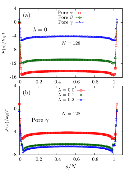
Figure 4: (a) Free energy $\mathcal{F}/k_{B}T$ as a function of $s/N$ for a flexible polymer ($\lambda=0$) of length $N=128$ translocating through various pores. (b) Free energy $\mathcal{F}/k_{B}T$ as a function of $s/N$ for a polymer of length $N=128$ translocating through Pore $\gamma$ for various values of chain stiffness $\lambda$. In plotting these figures, we have ignored the free energy contribution due to the external driving force ${\boldsymbol{F}}_{ext}=F\hat{\boldsymbol{x}}$.

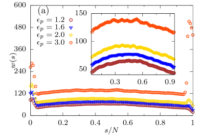
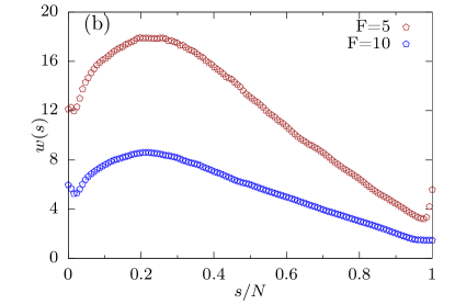
Figure 5: (a) The mean waiting times, $w({s})$, as a function of $s/N$ for a flexible polymer ($\lambda=0$) for various values of $\epsilon_{\rm pore}$ for Pore $\gamma$ at $F=1$. The inset shows the same data for the range $0.1\leq s/N\leq 0.9$. (b) The mean waiting times, $w({s})$, for higher values of external force $F=5$ and 10 for Pore $\alpha$ at $\epsilon_{pore}=1.2$. The sharp rise in $w(s)$ for the end monomers is completely washed off with increasing driving force.

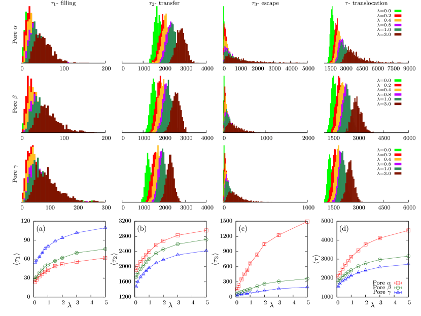
Figure 6: Translocation time statistics for semiflexible polymers with homogeneous bending rigidity. First, second and third rows : Translocation time distributions for pores $\alpha$, $\beta$ and $\gamma$ respectively, for $F=1.0$, as $\lambda$ is varied. Not only are the the three distributions different in their moments across the three pores, they also vary with varying $\lambda$. Fourth row : Average (a) filling time, $\langle\tau_{1}\rangle$ (b) transfer time, $\langle\tau_{2}\rangle$ , (c) escape time, $\langle\tau_{3}\rangle$ and (d) mean translocation time $\langle\tau\rangle$ as a function of $\lambda$. The error bars represent standard deviation of the mean.

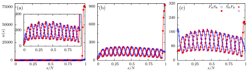
Figure 7: Waiting times for heteropolymers, $S_{8}F_{8}$ and $F_{8}S_{8}$, translocating through (a) Pore $\alpha$, (b) Pore $\beta$, and (c) Pore $\gamma$. The open and filled symbols represent flexible (F) and stiff (S) segments, respectively. The results for heteropolymers, $F_{8}S_{8}$ and $S_{8}F_{8}$, are shown by circles and diamonds, respectively.

In order to understand these features, we focus on the surface energetics of the various patterned pores. A comprehensive picture of the translocation process, which takes into account the pore-polymer interactions and entropic contributions, can be obtained by constructing a free energy landscape, $\mathcal{F}/k_{B}T$, in terms of the translocation coordinate $s$muthukumar2003 ; Katkar2014 . The translocation process is separated into three stages: (i) the pore filling, (ii) the transfer, and (iii) escape from the pore. At every stage, the free energy of the system has contributions from (i) pore-polymer interactions, ${\mathcal{F}}_{\textrm{pore}}$, (ii) polymer entropy, ${\mathcal{F}}_{\textrm{ent}}$, and (iii) energy due to the externally applied force, ${\mathcal{F}}_{\textrm{force}}$. In this analysis, we have neglected the contribution to the free energy due to the constant external force acting on every bead inside the pore, ${\mathcal{F}}_{\textrm{force}}$. The presence of this external force facilitates entry and exit of the polymer and is therefore expected to influence pore filling and escape stages. However, in this study, we restrict ourselves to small forces, where the effects of pore polymer interactions and polymer entropy are dominant. The free energy contribution due to pore-polymer interaction, $\mathcal{F}_{\textrm{pore}}(s)$, is obtained by summing over the LJ potential (Eq. 4) felt by each polymer bead (inside the pore) due to the pore beads. The entropic contribution for a chain with $s$ monomers on the cis(or trans) side is given by the entropy for a polymer with one end fixed to a wallmuthukumar2003 , $\mathcal{F}_{\textrm{ent}}(s)=k_{B}T(1-\Gamma)\ln(s)$, where $\Gamma=0.69$.

In the pore filling stage ($0<s<L$), $s$ monomers are inside the pore and remaining $N-s$ monomers are in the cis side. Then, $\mathcal{F}(s)=\mathcal{F}_{\textrm{pore}}(s)+\mathcal{F}_{\textrm{ent}}(N-s).$ In the transfer stage ($L<s<N$), $L$ monomers are inside the pore, $s-L$ are on the cis side and $N-s$ are on the trans side. Therefore, the free energy at this stage, $\mathcal{F}(s)=\mathcal{F}_{\textrm{pore}}(L)+\mathcal{F}_{\textrm{ent}}(N-s)+\mathcal{F}_{\textrm{ent}}(s-L).$ In the final stage $(N<s<N+L)$, $s-L$ monomers are on the trans side while $N+L-s$ monomers are inside the pore. At this stage, $\mathcal{F}(s)=\mathcal{F}_{\textrm{pore}}(N+L-s)+\mathcal{F}_{\textrm{ent}}(s-L)$. In Fig. 4(a), we have plotted the free energy $\mathcal{F}(s)/k_{B}T$ for a flexible polymer ($\lambda=0$) as a function of the translocation coordinate for translocation from Pores $\alpha$, $\beta$ and $\gamma$.

From Fig. 4(a) and the plot of the potential energy experienced by a chain monomer at any point along the axis of the pore due to the pore beads on either side (Fig. 1), it is clear that Pore $\alpha$ is an uniformly attractive pore. Although this makes it easier to pull the polymer inside the pore, the attractive interaction makes it difficult to exit the pore from the trans side for small external forces. Pore $\beta$ has a shallower well compared to Pore $\alpha$. Further, the free energy barrier at the trans end of the pore is significantly larger for Pore $\alpha$ than Pores $\beta$. Therefore, the mean waiting times for the end monomers are significantly less for Pore $\beta$ as compared to Pore $\alpha$. For Pore $\gamma$, which has a repulsive exit, this effect is the least. However, Pore $\gamma$ has a large repulsive exit and a short attractive entrance. Since the attractive entrance spreads over two monomers of the pore, only a few beads will be sucked inside the pore initially. Once it becomes energetically favorable for the first monomer to exit the pore by crossing the barrier, the inter chain interaction ensures that the monomers immediately adjacent to it are dragged out resulting in smaller waiting times successively for the initial beads. This is the cause of the dip in the waiting times for the first few monomers.

The free energy analysis can be extended for the case of a semiflexible polymer ($\lambda\neq 0$) by replacing the number of monomers $n$ in the entropic contributions with the number of Kuhn segments $n^{\prime}=n\sigma/\ell_{K}$, where $\ell_{K}=2\ell_{p}$ represents the Kuhn length gauthier . Within this approximate approach, we can explain qualitatively the observed dependencies of the translocation times on the stiffness $\lambda$ of the polymer. As observed in Fig. 4(b), $\mathcal{F}(s)/k_{B}T$ shows an increasing well depth as $\lambda$ is increased. This indicates that it become increasingly difficult to cross the free energy barrier at the trans end of the pore, resulting in increased translocation times with increasing stiffness.

In our simulations for extended pores, we choose $\epsilon_{pore}=1.2$ and $F=1$ to ensure that the effect of pore-polymer interactions, and hence the pore patterning, are dominant. Higher $\epsilon_{pore}$ increases the mean translocation time, while at high values of force, pore patterning effects are significantly reduced. In Fig. 5(a) we see that the mean waiting time for a monomer inside the pore increases with increasing $\epsilon_{\textrm{pore}}$. Further, the characteristic features near the cis and trans ends become even more prominent vindicating our earlier arguments. Increasing $F$, the mean waiting time drops sharply and the end features are completely washed out (Fig. 5(b)).

III.2 Translocation time distributions

In the light of the above free energy argument, it is useful to divide the total translocation time as $\tau=\tau_{1}+\tau_{2}+\tau_{3}$ luo2007prl ; Cohen2012 where (i) $\tau_{1}$ is the initial filling time, the time taken by the first monomer of the polymer to reach the exit without returning to the pore, (ii) $\tau_{2}$, the transfer time, the time taken from the exit of the first monomer into the trans-side to the entry of the last monomer from the cis-side and (iii) $\tau_{3}$, the escape time, the time between the entry of the last monomer in the pore and its escape to the trans-side. We compare the separate average time scales for filling, transfer and escape for the three different pore patterns to investigate the effect of changing pore-polymer interactions (Fig. 6).

Effect of stiffness. All time scales show a monotonic increase with increasing stiffness. This behavior is expected from the discussion of waiting times which increases with increasing $\lambda$. Note that, unlike a pore of unit length, the summation of mean waiting times for all monomers do not give the mean translocation time for an extended pore. However, when scaled by the pore length, the sum of mean waiting times still provide an excellent measure of the mean translocation time for such cases (data not shown).

Effect of pore patterning. Our simulation shows that $\langle\tau_{1}\rangle$ is the minimum for Pore $\alpha$ and maximum for Pore $\gamma$ for a fixed value of stiffness $\lambda$. From the free energy diagram, we note that for the initial filling process ($0<s<L$), the free energy falls sharpest for Pore $\alpha$. This indicates that filling is considerably easier for Pore $\alpha$ and less so for Pores $\beta$ and $\gamma$ which explains the simulation results. The free energy diagram also tells us that both transfer and escape are dictated by shallowness of the free energy landscape and the barrier experienced during the expulsion process of the polymer, both of which are maximum for Pore $\alpha$ and minimum for Pore $\gamma$. This is consistent with the observation of $\langle\tau_{2}\rangle$ and $\langle\tau_{3}\rangle$ for the three different pores at a given stiffness.

These results can be compared with those earlier observed for flexible chains Cohen2012 as a function of pore-polymer interaction strength, $\epsilon_{\textrm{pore}}$. As one would expect, the effect of varying $\epsilon_{\textrm{pore}}$ is quite drastic and was used to demonstrate sequencing Cohen2012 based on its variation. Our analysis on the other hand, clearly demonstrates the significant effect of chain stiffness on translocation time distributions for patterned pores without changing $\epsilon_{\textrm{pore}}$.

IV Heterogeneous translocation.

We next investigate the possibility of heteropolymer sequencing by passing them through multiple patterned pores. As elaborated in Sec II, we introduce heterogeneity by varying the stiffness of the polymer along the chain backbone. The heterogeneity introduced in our polymer model is periodic with alternate flexible ($\lambda=0$) and stiff ($\lambda\neq 0$) segments. Note that heteropolymer sequencing have been studied in the past using flexible polymers where the heterogeneity was introduced in a manner in which alternate polymer segments interacted with the pore Cohen2012 . In our analysis, we study the experimentally relevant scenario of varying bending rigidity in biopolymers. Due to this heterogeneity in stiffness, it is important to understand the effect of switching orientation of the polymer as it translocates from the cis to the trans side. We first discuss the effect of heterogeneity and orientation on mean waiting time and translocation time dynamics. Our choice of $\epsilon_{\textrm{pore}}=2$ and $\lambda=0.5$ for the stiff segment ensures a significant difference in the translocation times of the flexible and the stiff segments across different pores.

IV.1 Waiting times

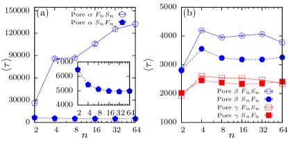
Figure 8: Average translocation time $\langle\tau\rangle$ as a function of block length $n$ (in log scale) for a polymer of length $N=128$ having alternate stiff (S) and flexible (F) segments. (a) Polymer translocating through Pore $\alpha$, and (b) Pores $\beta$ (circles) and $\gamma$ (squares). The results for polymer entering the pore through the stiff (flexible) end, represented by $S_{n}F_{n}$ ($F_{n}S_{n}$), are shown by filled (open) symbols. The inset in (a) shows the zoomed data for the case where the polymer enters the Pore $\alpha$ through the stiff end. The error bars represent standard deviation of the mean.

The effect of tension propagation in a polymer with periodically varying bending rigidity becomes clear when we look at the waiting time distribution. The distinct difference in the behavior of mean waiting times observed in Fig. 7, as opposed to earlier studies using heteropolymers of alternate stiff and flexible segments translocating through pores of unit length Haan2010 ; Adhikari2015 , are in the edge monomers where the pore synergetics becomes dominant. For the rest of the monomers, the oscillatory behavior displays the same characteristics. From waiting time distribution of monomers of a homogeneous polymer we know that (i) tension propagates faster for chains with increasing stiffness and hence (ii) leads to larger waiting times. In the case of heterogeneous polymers, tension propagates intermittently through blocks of stiff and flexible segments leading to the oscillations in the waiting time distribution Haan2010 ; Adhikari2015 . A stiff block has a larger waiting time, followed by a flexible block with lower waiting time and so on. When the orientation of the chain is reversed, the oscillations for $S_{n}F_{n}$ and $F_{n}S_{n}$ are exactly out of phase as expected. The waiting times for the end monomers of the chain however show distinct features for different orientations of the chain.

In sync with its homopolymer counterpart, the end chain dynamics of heteropolymers is strongly influenced by the pore-polymer interactions. For Pores $\alpha$ and $\beta$, the attractive interactions near the trans side of the pore dominate, leading to large waiting times. Evidently, the waiting times for the end monomers of the chain are significantly larger for Pore $\alpha$ compared to Pore $\beta$. This effect is significantly less for Pore $\gamma$ which has a repulsive exit.

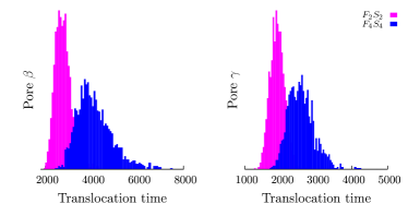
Figure 9: Translocation time distribution for sequences $(F_{2}S_{2})_{32}$ and $(F_{4}S_{4})_{16}$ translocating through Pores $\beta$ and $\gamma$.

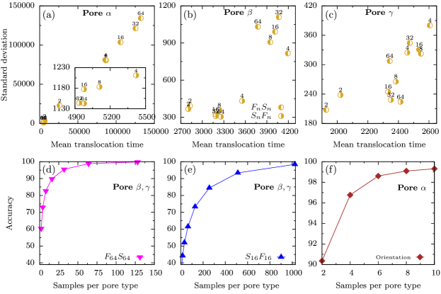
Figure 10: [(a) - (c)] Scatter plots showing mean and standard deviation of translocation times for Pores $\alpha$, $\beta$ and $\gamma$. The inset in (a) shows the zoomed bottom left portion for Pore $\alpha$. In each of these plots, the polymer entering the pore from the stiff end ($S_{n}F_{n}$) is shown by symbol half yellow filled circle (right), while the polymer entering from the flexible end ($F_{n}S_{n}$) is shown by half yellow filled circle (left). The accuracy of detecting heteropolymers (d) $F_{64}S_{64}$ (pink inverted triangles) and (e) $S_{16}F_{16}$ (blue triangles) through Pores $\beta$ and $\gamma$. (f) Accuracy of detection by including Pore $\alpha$ to distinguish orientation of the heteropolymer $S_{16}F_{16}$.

The end chain dynamics for the reversed conformation $S_{n}F_{n}$ is not significantly affected by these interactions. Pore $\alpha$ due to the large potential barrier does make it difficult for the end monomers to exit the pore leading to larger waiting times. However, the waiting times are considerably less compared to $F_{n}S_{n}$. Pore $\beta$ and $\gamma$ are largely unaffected. This is expected from our earlier analysis of larger waiting times for stiffer chains. Polymer in the conformation $S_{n}F_{n}$ enters the pore with the stiffer block entering first followed by a flexible block. This implies that a flexible block exits the pore last in this conformation. In contrast, in the conformation $F_{n}S_{n}$, it is a stiff block which exits the pore last from the trans side in the translocation process leading to much larger waiting times.

We argue that these distinguishing features observed for the end monomers and dominated by the pore synergetics, result in distinct translocation time distributions for different pores. We use this to effectively distinguish heteropolymers with varying bending rigidity using a statistical analysis based on the moments of the distributions.

IV.2 Average translocation time

The mean translocation times for the heteropolymers as they pass through the patterned pores, mimic the behavior of the mean waiting times of individual monomers. For pore $\alpha$, the difference in the mean waiting times for the two different orientations is significant and increases with increasing block length $n$ (Fig. 8). This is a result of the difference in waiting times of the end monomers during exit. Also note that for longer block lengths the tension can propagate over larger lengths of the polymer uninterrupted. For pore $\beta$, the effect of the longer waiting times for end monomers on the total translocation time is less significant while for pore $\gamma$, it is effectively the same for both orientations of the polymer during translocation.

IV.3 Sequencing of polynulceotide with varying bending rigidity

The sensitivity of the translocation dynamics on the varying bending rigidity of heteropolymers and the patterning of pores opens up the possibility of sequencing heteropolymers based on their unique translocation time statistical properties. For example, in Fig. 9 we show the translocation time distribution for sequences $(F_{2}S_{2})_{32}$ and $(F_{4}S_{4})_{16}$ for pores $\beta$ and $\gamma$. These translocation time distributions exhibit distinct features corresponding to the variation in the block lengths of the heteropolymer. However, for certain heteropolymers, there could be significant overlap in the distribution. We calculate the mean translocation time ($\langle\tau\rangle$) and the standard deviation ($\sqrt{\langle\tau^{2}\rangle-\langle\tau\rangle^{2}}$) of the translocation times from these distributions and construct scatter plots for each pore type as shown in Fig. 10. The scatter plots reveal several interesting features. For example, Pore $\gamma$ cannot distinguish between $(S_{32}F_{32})_{2}$ and $(S_{64}F_{64})_{1}$, but Pore $\beta$ can. Similarly, Pore $\beta$ cannot distinguish between $(S_{2}F_{2})_{32}$ and $(F_{2}S_{2})_{32}$, but Pore $\gamma$ can. These differences in the scatter plots for the various pores, marking the mean and standard deviation for each sequence, clearly shows that a combination of translocation time measurements from multiple pores could be utilized to differentiate and identify sequences with a relatively small number of samples per pore type, which would otherwise be difficult to distinguish using measurements from a single pore.

Our simulation methodology for sequence detection is as follows. We choose a sequence of the heteropolymer (say $S_{k}F_{k}$, with a specific orientation) from the set of all available sequences (defined as the training set) used to plot Figs. 10(a-c) and call it an “unknown” sequence. This sequence is then passed through a single pore of $\alpha$, $\beta$ or $\gamma$ type. For each pore type, the heteropolymer is passed multiple times and successful translocation events are registered (say $m$). For every attempted translocation, the chain configuration of the heteropolymer is chosen from the equilibrated configurations obtained in accordance with the simulation strategy discussed before (Sec. II). Having registered the successful translocation events across each pore, the mean translocation time and standard deviation are calculated for each pore type, which correspond to respective points in the scatter plots. These numbers are then compared with those of the training set for the corresponding pore using a “distance” metric. The larger the distance between the point corresponding to the “unknown” sequence is from a particular known sequence in the scatter plot, the greater is the relative error for that sequence. The total error, which is the sum of the distance from a particular known sequence in all the plots, is minimized to predict the “unknown” sequence. If the predicted sequence matches the sequence we started with, then this marks a successful detection.

The ratio of the number of times a sequence is correctly detected to the total number of attempts, gives the accuracy of the measurement process (see Fig. 10(d)-(f)). The samples per pore type merely indicate the number of registered successful translocation events chosen for the unknown sequence across each pore type. Evidently, if we use a very large number of samples for a given pore type, the sequence detection would be accurate. However, this scheme suggests that a combination of different pore types gives very high accuracy of prediction for a relatively small number of copies of each pore. In Fig. 10, we have used the statistical data for only two pore types, Pores $\beta$ and $\gamma$, to test our hypothesis. Employing the above scheme we found, for example, that the accuracy of detection for the sequence, $F_{64}S_{64}$ (Fig. 10(d)), reaches $100\%$, even for $~{}\sim 130$ samples per pore type. It is important to note that in our method of sequence detection, we have used only the first two moments of the probability distribution of translocation times. As observed from the results of the distributions, this is far from accurate. Inclusion of higher moments would most definitely improve the accuracy of the scheme and lead to a more rapid convergence. Further, our method has considered only a few possible pore types. It would be interesting to design pores leading to even more distinguishable translocation time statistics, which when used in conjunction with varying semiflexibility across the polymer backbone, would lead to enhanced sequence detection.

From the set of pores chosen for this study, it is evident that for Pore $\alpha$, there is an order of magnitude difference in the translocation times of stiff and flexible segments. Therefore, this pore is an ideal candidate to detect the difference in orientation between $S_{k}F_{k}$ and $F_{k}S_{k}$ and make the detection process even more precise. Indeed, we find that the accuracy of detecting the correct orientation is almost 100 percent even for a small number of copies of Pore $\alpha$ (Fig. 10(f)). We would like to stress that it is not necessary to distinguish the orientation of the polymer before passing them through the pores. Our statistical analysis simply suggest that it requires far less samples per pore type if we manage to do so.

Our result needs to be compared with the case where heterogeneous segments were distinguished by their relative interactions with the pore Cohen2012 . It turns out that in such a scenario, the translocation time distributions have sharper and more distinguished features, leading to better sequencing accuracy. However, as argued before, structural heterogeneity of a polymer is an experimentally relevant scenario and our analysis shows that using different patterned pores can lead to efficient sequencing strategies for such cases. It is important to note that our analysis is robust with respect to changes in pore width and the length of the polymer (see the supplementary material).

The sequencing theme outlined above, can be experimentally realized using fabricated nanofluidic channels with surface decoration. Arrays of nanochannels interfaced with microfludic loading channels have been shown to be a highly parallel platform for the restriction mapping of DNA  Persson2010 ; Reisner2010 ; Schoch2008 . The first task is to construct the set of translocation time distributions for known sequences. This requires passing sequences with a particular orientation multiple times through these functionally modified nanofluidic channels. Solid state nanopores are other highly plausible candidates to achieve the same. With the training set characterised, the sequencing of heteropolymers with “unknown” sequences can be efficiently achieved in limited time by passing them through these channels using our purely statistical analysis. The detection of the orientation of the polymer could be achieved using a fluorescent dye on either the stiff or flexible end of the polymerJu1995 .

V Summary

We have shown how statistical fluctuations in the translocation time dynamics could be efficiently used to sense sequence dependent bending rigidity of biopolymers. The mean waiting times, $w(s)$, of the beads of the polymer and correspondingly the mean translocation times, gives extensive information of the translocation dynamics. The strong dependence of these properties on the bending rigidity of the polymer and the distinguishable translocation time statistics generated due to different patterned stickiness, allows us to efficiently detect polymers with varying bending rigidity by combining readouts from multiple pores for rapid convergence. For extended pores, the breakup of the total translocation time into the filling, transfer and escape times proves useful and in this context reveal interesting features for semiflexible polymer translocation hitherto unobserved for pores of unit length. The effect of changing the external bias and pore length are important aspects of future study.

Supplementary Material

See supplementary material for the robustness of our sequence detection scheme with respect to changes in the pore width and the length of the polymer.

Supplementary Material

The pore widths used in our study compare favorably with experimental scenarios. The units of energy, length and mass are set by $\epsilon$, $\sigma$, and $m$, respectively. This sets the unit of time as $(m\sigma^{2}/\epsilon)^{1/2}$ and that of force as $\epsilon/\sigma$. Following earlier studies  Luo2008 ; Cohen2012 , we assume the bead size in our coarse-grained polymer model as $\sigma=1.5$ nm. This is equal to the Kuhn length of a single-stranded DNA, which is approximately three nucleotide bases. Hence the mass of the bead is $m\approx 936$ amu (given that the mass of a base in DNA is $\approx 312$ amu) and charge of the bead $q\approx 0.3$ e (each base having a charge of 0.1 e effectively). To allow comparison with known results, we set $\zeta=0.7$ and $k_{B}T=1.2$. At $T=295$ K, the interaction strength is given by $\epsilon=k_{B}T/1.2\approx 3.4\times 10^{-21}$ J, which gives a time scale of $(m\sigma^{2}/\epsilon)^{1/2}\approx 30$ ps and force scale of $\epsilon/\sigma\approx 2.4$ pN. Therefore, an external driving force of $F=1.0$ corresponds to a voltage range $V=FL/q\approx 190-380$ mV across the pores. In these units, a pore width of $W=2.25$ corresponds to $\sim 3.5$nm which is not unphysical. The internal constriction of the $\alpha$ Hemolysin pore is $\sim 1.5$nm. Solid state nanopores of width $3-10$nm are now routinely used.

To test the robustness of the method proposed in the main paper, we apply it to heteropolymer chains consisting of stiff and flexible segments ($S_{n}F_{n}$ and $F_{n}S_{n}$) of length $N=32$ translocating through patterned Pores $\beta$ and $\gamma$ having pore width $W=3$. We choose $\epsilon_{\textrm{pore}}=2$ for Pore $\beta$ and $\epsilon_{\textrm{pore}}=3$ for $\gamma$. All other simulation parameter values are the same as in the main paper. We construct scatter plot by calculating the mean translocation time and standard deviation obtained from 2000 successful translocation events. These plots are shown in Fig. S1(a) and  S1(b) for Pores $\beta$ and $\gamma$, respectively. Figures S1(c) and (d) show the accuracy of detection for sequences $F_{2}S_{2}$ and $S_{8}F_{8}$, respectively. For sequence $F_{2}S_{2}$, the accuracy reaches $100\%$, even for $~{}\sim 25$ samples per pore type. This shows that our analysis is robust enough with respect to changes in the pore width, and the polymer length and an unknown sequence could be detected to a high accuracy with a relatively small number of samples per pore type.

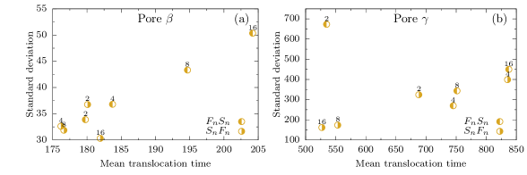
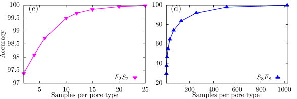
Figure S1: (a) and (b) Plot of mean translocation time and standard deviation, obtained from 2000 successful translocation events, for a polymer of length $N=32$ translocating through pore of width $W=3$. The polymer entering the pore from the stiff end ($S_{n}F_{n}$) is shown by symbol $\RIGHTcircle$ while the polymer entering from the flexible end ($F_{n}S_{n}$) is shown by $\LEFTcircle$. The accuracy of detecting heteropolymers (c) $F_{2}S_{2}$ ($\blacktriangledown$) and (d) $S_{8}F_{8}$ ($\blacktriangle$) through Pores $\beta$ and $\gamma$.

References

- (1) J. Frank and R. L. Gonzalez Jr., Ann. Rev. Biochem. 79, 381 (2010).
- (2) H. Salman et. al., Proc. Natl. Acad. Sci. USA 98, 7247 (2001).
- (3) R. F. Service, Science 311, 1544 (2006).
- (4) J. Lagerqvist, M. Zwolak & M. Di Ventra, Nano Lett. 6, 779 (2006).
- (5) D. Branton et al. Nature Biotechnol. 26, 1146 (2008).
- (6) J. Shendure and H. Ji, Nature Biotechnol. 26, 1135 (2008).
- (7) J. A. Schloss, Natute Biotechnol. 26, 1113 (2008).
- (8) F. Persson and J. O. Tegenfeldt, Chem. Soc. Rev. 39, 985 (2010).
- (9) M. Zwolak and M. Di Ventra, Rev. Mod. Phys. 80, 141 (2008).
- (10) S. K. Min, W. Y. Kim, Y. Cho and K. S. Kim, Nature Nanotechnol. 6, 162 (2011).
- (11) D. W. Deamer and D. Branton, Acc. Chem. Res. 35, 817 (2002).
- (12) J. J. Kasianowicz, E. Brandin, D. Branton and D. W. Deamer, Proc. Natl. Acad. Sci. U.S.A. 93, 13770 (1996).
- (13) O. Braha et al., Chem. Biol. 4, 497 (1997).
- (14) M. Akeson, D. Branton, J. J. Kasianowicz, E. Brandin and D. W. Deamer, Biophys. J. 77, 3227 (1999).
- (15) A. Meller, L. Nivon, E. Brandin, J. Golovchenko and D. Branton, Proc. Natl. Acad. Sci. USA 97, 1079 (2000).
- (16) A. Meller, L. Nivon and D. Branton, Phys. Rev. Lett. 86, 3435 (2001).
- (17) A. Meller, J. Phys. Condens. Matter 15, R581 (2003).
- (18) G. Maglia, M. R. Rincon Restrepo, E. Mikhailova, and H. Bayley, Proc. Natl. Acad. Sci. USA 105, 19720, (2008).
- (19) M. Muthukumar, J. Chem. Phys. 111, 10371 (1999).
- (20) D. K. Lubensky and D. R. Nelson, Biophys. J. 77, 1824 (1999).
- (21) I. Huopaniemi, K. Luo, T. Ala-Nissila and S. C. Ying, J. Chem. Phys. 125, 124901 (2006).
- (22) M. Muthukumar and C. Y. Kong, Proc. Natl. Acad. Sci. USA 103, 5273 (2006).
- (23) J. M. Polson and A. C. M. McCaffrey, J. Chem. Phys. 138, 174902 (2013).
- (24) S. Matysiak, A. Montesi, M. Pasquali, A. B. Kolomeisky and C. Clementi, Phys. Rev. Lett. 96, 118103 (2006).
- (25) K. Luo, T. Ala-Nissila, S. C. Ying and A. Bhattacharya, Phys. Rev. Lett. 99, 148102 (2007).
- (26) K. Luo, T. Ala-Nissila, S. C. Ying and A. Bhattacharya, Phys. Rev. E 78, 061918 (2008).
- (27) K. Luo, T. Ala-Nissila, S. C. Ying and A. Bhattacharya, Phys. Rev. Lett. 100, 058101 (2008).
- (28) K. Luo, T. Ala-Nissila, S-Chen Ying and Aniket Bhattacharya J. Chem. Phys. 126, 145101 (2007).
- (29) S. Mirigian, Y. Wang and M. Muthukumar J. Chem. Phys. 137, 064904 (2012).
- (30) M. G. Gauthier and G. W. Slater, J. Chem. Phys. 128, 175103 (2008).
- (31) B. Luan et. al., Phys. Rev. Lett. 104, 238103 (2010).
- (32) A. Nikoubashman and C. N. Likos, J. Chem. Phys. 133, 074901 (2010).
- (33) W. Sung and P. J. Park, Phys. Rev. Lett. 77, 783 (1996).
- (34) M. Muthukumar, Phys. Rev. Lett. 86, 3188 (2001).
- (35) J. Chuang, Y. Kantor, Y. and M. Kardar, Phys. Rev. E 65, 011802 (2001).
- (36) M. Muthukumar, J. Chem. Phys. 118, 5174 (2003).
- (37) R. Metzler and J. Klafter, Biophys. J. 85, 2776 (2003).
- (38) E. Slonkina and A. B. Kolomeisky, J. Chem. Phys. 118, 7112 (2003).
- (39) Y. Kantor and M. Kardar, Phys. Rev. E 69, 021806 (2004).
- (40) A. Milchev, K. Binder and A. Bhattacharya, J. Chem. Phys. 121, 6042 (2004).
- (41) U. Gerland, R. Bundschuh and T. Hwa, Phys. Biol. 1, 19 (2004).
- (42) A. Gopinathan and Y. W. Kim, Phys. Rev. Lett. 99, 228106 (2007).
- (43) C. T. A. Wong and M. Muthukumar, J. Chem. Phys. 133, 045101 (2010).
- (44) A. Milchev, J. Phys. Condens. Matter 23, 103101 (2011).
- (45) R. H. Abdolvahab, M. R. Ejtehadi, and R. Metzler, Phys. Rev. E 83, 011902 (2011).
- (46) J. A. Cohen, A. Chaudhuri, and R. Golestanian Phys. Rev. Lett. 107, 238102 (2011).
- (47) T. Sakaue, Phys. Rev. E 76, 021803 (2007).
- (48) T. Sakaue, Phys. Rev. E 81, 041808 (2010).
- (49) T. Saito and T. Sakaue, Eur. Phys. J. E 34, 135 (2011).
- (50) P. Rowghanian and A. Y. Grosberg, J. Phys. Chem. B 115, 14127 (2011).
- (51) J. L. A. Dubbeldam, V. G. Rostiashvili, A. Milchev, and T. A. Vilgis, Phys. Rev. E 85, 041801 (2012).
- (52) T. Ikonen, A. Bhattacharya, T. Ala-Nissila and W. Sung, Phys. Rev. E 85, 051803 (2012).
- (53) T. Ikonen, A. Bhattacharya, T. Ala-Nissila and W. Sung, J. Chem. Phys. 137, 085101 (2012).
- (54) J. Sarabadani, T. Ikonen and T. Ala-Nissila, J. Chem. Phys. 141, 214907 (2014).
- (55) J. Sarabadani, T. Ikonen, H.Mökkönen, T Ala-Nissila, S. Carson and M. Wanunu, Scientific Rep. 7, 7423 (2017).
- (56) V. V. Lehtola, R. P. Linna, and K. Kaski, EPL 85, 58006 (2009).
- (57) H. W. de Haan, and G. W. Slater, Phys. Rev. Lett. 110, 048101 (2013).
- (58) A. Bhattacharya, Polymer Science, Ser. C 55, 60 (2013).
- (59) R. Adhikari and A. Bhattacharya, J. Chem. Phys., 138, 204909 (2013).
- (60) R. Adhikari and A. Bhattacharya, Europhys. Lett., 109, 38001 (2015).
- (61) J. A. Cohen, A. Chaudhuri, and R. Golestanian, Phys. Rev. X, 2, 021002 (2012).
- (62) J. A. Cohen, A. Chaudhuri, and R. Golestanian, J. Chem. Phys. 137, 204911 (2012).
- (63) H. H. Katkar and M. Muthukumar, J. Chem. Phys. 140, 135102 (2014).
- (64) A. Dhar and D. Chaudhuri, Phys. Rev. Lett. 89, 065502 (2002).
- (65) J. Wilhelm and E. Frey, Phys. Rev. Lett. 77, 2581 (1996).
- (66) J. Widom, Q Rev Biophys 34, 269 (2001).
- (67) A. A. Travers, Philos Trans Roy Soc A 362, 1423 (2004).
- (68) S. Geggier and A. Vologodskii, Proc. Natl. Acad. Sci USA 107, 15421 (2010).
- (69) C. Branden and J. Tooze, Introduction of Protein Structure (Garland Publishing, New York, 1998).
- (70) M. Lee, B. K. Cho, and W. C Zin, Chem. Rev. 101, 3869 (2001).
- (71) E. Stellwagen, Y. Lu, and N. Stellwagen, Biochemistry 42, 11 745 (2003).
- (72) S. W. Kowalczyk, A. R. Hall, and C. Dekker, Nano Lett. 10, 324 (2010).
- (73) A. J. Storm, J. H. Chen, X. S. Ling, H. W. Zandbergen and C. Dekker, Nature Mater. 2, 537 (2003).
- (74) M. J. Kim, M. Wanunu, D. C. Bell and A. Meller, Adv. Mater. 18, 3149 (2006).
- (75) T. Ohshiro and Y. Umezawa, Proc. Natl. Acad. Sci. USA 103, 1014 (2006).
- (76) S. M. Iqbal, D. Akin and R. Bashir, Nature Nanotechnol. 2, 243 (2007).
- (77) M. Wanunu and A. Meller, Nano Lett. 7, 1580 (2007).
- (78) P. Chen et al., Nano Lett. 4, 1333 (2004).
- (79) V. Tabard-Cossa, D. Trivedi, M. Wiggin, N. N. Jetha and A. Marziali, Nanotechnology 18, 305505 (2007).
- (80) W. Reisner et al., Proc. Natl. Acad. Sci. USA 107, 13294 (2010).
- (81) R. B. Schoch, J. Han and P. Renaud, Rev. Mod. Phys. 80, 839 (2008).
- (82) J. Ju, C. Ruan, C. W. Fuller, A. N. Glazer and R. A. Mathies, Proc. Natl. Acad. Sci. USA 92, 4347 (1995).

References

- (1) K. Luo, T. Ala-Nissila, S. C. Ying and A. Bhattacharya, Phys. Rev. Lett. 100, 058101 (2008).
- (2) J. A. Cohen, A. Chaudhuri, and R. Golestanian, Phys. Rev. X, 2, 021002 (2012).