Grade Prediction with Temporal Course-wise Influence

Abstract

There is a critical need to develop new educational technology applications that analyze the data collected by universities to ensure that students graduate in a timely fashion (4 to 6 years); and they are well prepared for jobs in their respective fields of study. In this paper, we present a novel approach for analyzing historical educational records from a large, public university to perform next-term grade prediction; i.e., to estimate the grades that a student will get in a course that he/she will enroll in the next term. Accurate next-term grade prediction holds the promise for better student degree planning, personalized advising and automated interventions to ensure that students stay on track in their chosen degree program and graduate on time. We present a factorization-based approach called Matrix Factorization with Temporal Course-wise Influence that incorporates course-wise influence effects and temporal effects for grade prediction. In this model, students and courses are represented in a latent “knowledge” space. The grade of a student on a course is modeled as the similarity of their latent representation in the “knowledge” space. Course-wise influence is considered as an additional factor in the grade prediction. Our experimental results show that the proposed method outperforms several baseline approaches and infer meaningful patterns between pairs of courses within academic programs.

1 Introduction

Data analytics is at the forefront of innovation in several of today’s popular Educational Technologies (EdTech) [17]. Currently, one of the grand challenges facing higher education is the problem of student retention and graduation [19]. There is a critical need to develop new EdTech applications that analyze the data collected by universities to ensure that students graduate in a timely fashion (4 to 6 years), and they are well prepared for jobs in their respective fields of study. To this end, several universities deploy a suite of software and tools. For example, degree planners assist students in deciding their majors or fields of study, choosing the sequence of courses within their chosen major and providing advice for achieving career and learning objectives. Early warning systems [27] inform advisors/students of progress, and additionally provide cues for intervention when students are at the risk of failing one or more courses and dropping out of their program of study. In this work, we focus on the problem of next-term grade prediction where the goal is to predict the grade that a student is expected to obtain in a course that he/she may enroll in the next term (future).

In the past few years, several algorithms have been developed to analyze educational data, including Matrix Factorization (MF) algorithms inspired from recommender system research. MF methods decompose the student-course (or student-task) grade matrix into two low-rank matrices, and then the prediction of the grade for a student on an untaken course is calculated as the product of the corresponding vectors in the two decomposed matrices [22, 11]. Traditional MF algorithms have shown a strong ability to deal with sparse datasets [14] and their extensions have incorporated temporal and dynamic information [12]. In our setting, we consider that a student’s knowledge is continuously being enriched while taking a sequence of courses; and it is important to incorporate this dynamic influence of sequential courses within our models. Therefore, we present a novel approach referred as Matrix Factorization with Temporal Course-wise Influence (MFTCI) model to predict next term student grades. MFTCI considers that a student’s grade on a certain course is determined by two components: (i) the student’s competence with respect to each course’s topics, content and requirement, etc., and (ii) student’s previous performance over other courses. We performed a comprehensive set of experiments on various datasets. The experimental results show that the proposed method outperforms several state-of-the-art methods. The main contributions of our work in this paper are as follows:

1. We model and incorporate temporal course-wise influence in addition to matrix factorization for grade prediction. Our experimental results demonstrate significant improvement from course-wise influence.

2. Our model successfully captures meaningful course-wise influences which correlate to the course content.

3. The learned influences between pairs of courses help in understanding pre-requisite structures within programs and tuning academic program chains.

2 Related Work

Over the past few years, several methods have been developed to model student behavior and academic performance  [2, 9], and they gain improvement of learning outcomes [21]. Methods influenced by Recommender System (RS) research [1], including Collaborative Filtering (CF) [18] and Matrix Factorization  [13], have attracted increasing attention in educational mining applications which relate to student grade prediction [32] and in-class assessment prediction [8]. Sweeney et. al. [31, 30] performed an extensive study of several recommender system approaches including SVD, SVD-kNN and Factorization Machine (FM) to predict next-term grade performance. Inspired by content-based recommendation [20] approaches, Polyzou et. al. [23] addressed the future course grade prediction problem with three approaches: course-specific regression, student-specific regression and course-specific matrix factorization. Moreover, neighborhood-based CF approaches [25, 4, 6] predict grades based on the student similarities, i.e., they first identify similar students and use their grades to estimate the grades of the students with similar profiles.

In order to capture the changing of user dynamics over time in RS, various dynamic models have been developed. Many of such models are based on Matrix Factorization and state space models. Sun et. al. [28, 29] model user preference change using a state space model on latent user factors, and estimate user factors over time using noncausal Kalman filters. Similarly, Chua et.al. [5] apply Linear Dynamical Systems (LDS) on Non-negative Matrix Factorization (NMF) to model user dynamics. Ju et. al. [12] encapsulate the temporal relationships within a Non-negative matrix formulation. Zhang et. al. [34] learn an explicit transition matrix over the latent factors for each user, and estimate the user and item latent factors and the transition matrices within a Bayesian framework. Other popular methods for dynamic modeling include time-weighting similarity decaying [7], tensor factorization [33] and point processes [16]. The method proposed in this paper tackle the challenges of next-term grade prediction which relates to the evolvement of student knowledge over taking a sequence of courses. Our key contribution involves how we incorporate the temporal course-wise relationships within a MF approach. Additionally, the proposed approach learns pairwise relationships between courses that can help in understanding pre-requisite structures within programs and tuning academic program chains.

3 Preliminaries

3.1 Problem Statement and Notations

Formally, student-course grades will be represented by a series of matrices {G₁, G₂, …, G_T} for $T$ terms. Each row of $G_{t}$ represents a student, each column of $G_{t}$ represents a course, and each value in $G_{t}$, denoted as $g_{s,c}^{t}$, represents a grade that student $s$ got on course $c$ in term $t$ ($g_{s,c}^{t}\in(0,4]$, $g_{s,c}^{t}=0$ indicates that student $s$ did not take the course $c$ in term $t$. We add a small value to failing grade to distinguish 0 score from such situation.). Student-course grades up to the $t_{th}$ term will be represented by G^t=$\sum_{i=1}^{t}$G_i with size of $n\times m$, where $n$ is the number of students and $m$ is the number of courses. Given the database of (student, course, grade) up to term $(T-1)$ (i.e., G^T-1), the next-term grade prediction problem is to predict grades for each student on courses they might enroll in the next term $T$. To simplify the notations, if not specifically stated in this paper, we will use $g_{s,c}$ to denote $g^{t}_{s,c}$. Our testing set is then (student, course, grade) triples in the $T_{th}$ term, represented by matrix G_T. Rows from the grade matrices representing a student $s$ will simply be represented as $G(s,:)$ and the specific courses that student has a grade for in this row can be given by $c^{\prime}\in G(s,:)$.

In this paper, all vectors (e.g., $\mathbf{u}_{s}^{\mathsf{T}}$ and $\mathbf{v}_{c}$) are represented by bold lower-case letters and all matrices (e.g., $A$) are represented by upper-case letters. Column vectors are represented by having the transpose supscript^T, otherwise by default they are row vectors. A predicted/approximated value is denoted by having a $\tilde{\ }$ head.

4 Methods

4.1 MF with Temporal Course-wise Influence

We consider the student $s$’ grade on a certain course $c$, denoted as $g_{s,c}$, as determined by two factors. The first factor is the student $s$’ competence with respect to the course $c$’s topics, content and requirement. This is modeled through a latent factor model, in which $s$’ competence is captured using a size-$k$ latent factor $\mathbf{u}_{s}$, $c$’s topics and contents are captured using a size-$k$ latent factor $\mathbf{v}_{c}$ in the same latent space as $\mathbf{u}_{s}$. Then the competence of $s$ over $c$ is modeled by the “similarity” between $\mathbf{u}_{s}$ and $\mathbf{v}_{c}$ via their dot product (i.e., $\mathbf{u}_{s}^{\mathsf{T}}\mathbf{v}_{c}$).

The second factor is the previous performance of student $s$ over other courses. We hypothesize that if course $c^{\prime}$ has a positive influence on course $c$, and student $s$ achieved a high grade on $c^{\prime}$, then $s$ tends to have a high grade on $c$. Under this hypothesis, we model this second factor as a product between the performance of student on a previous “related” course where the pairwise course relationships are learned in our formulation. Note that we consider this pairwise course influence as time independent, i.e., the influence of one course over another does not change over time. However, the impact from previous performance/grades can be modeled using a decay function over time. Taking these two factors, the estimated grade is given as follows:

$$\tilde{g}_{s,c} =\mathbf{u}_{s}^{\mathsf{T}}\mathbf{v}_{c}$$ (1)

$$+\underbrace{e^{-\alpha}\frac{\sum_{c^{\prime}\in G_{T-1}(s,:)}A(c^{\prime},c)g_{s,c^{\prime}}}{|G_{T-1}(s,:)|}}_{\Delta(T-1)}$$

$$+\underbrace{e^{-2\alpha}\frac{\sum_{c^{\prime\prime}\in G_{T-2}(s,:)}A(c^{\prime\prime},c)g_{s,c^{\prime\prime}}}{|G_{T-2}(s,:)|}}_{\Delta(T-2)},$$

in which $A(c^{\prime},c)$ is the influence of $c^{\prime}$ on $c$, $G_{T-1}(s,:)$/$G_{T-2}(s,:)$ is the subset of courses out of all courses that $s$ has taken in the first/second previous terms, $|G_{T-1}(s,:)|$/$|G_{T-2}(s,:)|$ is the number of such taken courses. $e^{-\alpha}$/$e^{-2\alpha}$ denote the time-decay factors. In Equation 1, we consider previous two terms. More previous terms can be included with even stronger time-decay factors. Given the grade estimation as in Equation 1, we formulate the grade prediction problem for term $T$ as the following optimization problem,

$$\underset{U,V,A}{\min} \frac{1}{2}\sum_{s,c}(g_{s,c}-\tilde{g}_{s,c})^{2}+\frac{\gamma}{2}(\|U\|_{F}^{2}+\|V\|_{F}^{2})$$

$$+\tau\|A\|_{*}+\lambda\|A\|_{\ell_{1}}$$

$$\text{s.t., }A\geq 0$$

where $U$ and $V$ are the latent non-negative student factors and course factors, respectively; $\|A\|_{*}$ is the nuclear norm of $A$, which will induce an $A$ of low rank; and $\|A\|_{\ell_{1}}$ is the $\ell_{1}$ norm of $A$, which will introduce sparsity in $A$. In addition, the non-negativity constraint on $A$ is to enforce only positive influence across courses.

4.1.1 Optimization Algorithm of MFTCI

We apply the ADMM [3] technique for Equation 4.1 by reformulating the optimization problem as follows,

$$\underset{U,V,A,U_{1},U_{2},Z_{1},Z_{2}}{\min}\ \frac{1}{2}\sum_{s,c}(g_{s,c}-\tilde{g}_{s,c})^{2}+\frac{\gamma}{2}(\|U\|_{F}^{2}+\|V\|_{F}^{2})$$

$$+\tau\|Z_{1}\|_{*}+\lambda\|Z_{2}\|_{\ell_{1}}$$

$$+\frac{\rho}{2}(\|A-Z_{1}\|_{F}^{2}+\|A-Z_{2}\|_{F}^{2})$$

$$+\rho(tr(U_{1}^{\mathsf{T}}(A-Z_{1})))$$

$$+\rho(tr(U_{2}^{\mathsf{T}}(A-Z_{2})))$$

s.t., $$A\geq 0$$

where $Z_{1}$ and $Z_{2}$ are two auxiliary variables, and $U_{1}$ and $U_{2}$ are two dual variables. All the variables are solved via an alternating approach as follows.

Step 1: Update $U$ and $V$

Fixing all the other variables and solving for $U$ and $V$, the problem becomes a classical matrix factorization problem:

$$\underset{U,V}{\min}\ \frac{1}{2}\sum_{s,c}(f_{s,c}-\mathbf{u}_{s}^{\mathsf{T}}\mathbf{v}_{c})^{2}+\frac{\gamma}{2}(\sum_{s}\|u_{s}\|_{2}^{2}+\sum_{c}\|v_{c}\|_{2}^{2})$$ (2)

where $f_{s,c}=g_{s,c}-\Delta(T-1)-\Delta(T-2)$ (See Eq 1). The matrix factorization problem can be solved using alternating minimization.

Step 2: Update $A$

Fixing all the other variables and solving for $A$, the problem becomes

$$\underset{A}{\min}\ \frac{1}{2}\sum_{s,c}(g_{s,c}-\tilde{g}_{s,c})^{2}+\frac{\rho}{2}(\|A-Z_{1}\|_{F}^{2}+\|A-Z_{2}\|_{F}^{2})$$

$$+\rho(tr(U_{1}^{\mathsf{T}}(A-Z_{1})))+\rho(tr(U_{2}^{\mathsf{T}}(A-Z_{2})))$$

s.t., $$A\geq 0$$

Using the gradient descent, the elements in $A$ can be updated as follows.

$$A (c_{i},c_{j})=A(c_{i},c_{j})-lr\times[\rho(A(c_{i},c_{j})-Z_{1}(c_{i},c_{j}))$$ (3)

$$+\rho(A(c_{i},c_{j})-Z_{2}(c_{i},c_{j}))+\rho U_{1}(c_{i},c_{j})+\rho U_{2}(c_{i},c_{j})$$

$$-\sum_{s,c_{j}}(g_{s,c_{j}}-\tilde{g}_{s,c_{j}})$$

$$\times\begin{cases}\frac{e^{-\alpha}}{|G_{T-1}(s,:)|}g_{s,c_{i}}\quad\text{(if $c_{i}$ is taken in term $T-1$)}\\ \frac{e^{-2\alpha}}{|G_{T-2}(s,:)|}g_{s,c_{i}}\quad\text{(if $c_{i}$ is taken in term $T-2$)}]\end{cases}$$

with projection into $[0,+\infty)$, where $lr$ is a learning rate.

Step 3: Update $Z_{1}$ and $Z_{2}$

For $Z_{1}$, the problem becomes

$$\underset{Z_{1}}{\min}\ \tau\|Z_{1}\|_{*}+\frac{\rho}{2}\|A-Z_{1}\|_{F}^{2}+\rho(tr(U_{1}^{\mathsf{T}}(A-Z_{1})))$$ (4)

The closed-form solution of this problem is

$$Z_{1}=S_{\frac{\tau}{\rho}}(A+U_{1})$$ (5)

where $S_{\alpha}(X)$ is a soft-thresholding function that shrinks the singular values of $X$ with a threshold $\alpha$, that is,

$$S_{\alpha}(X)=U\text{diag}((\Sigma-\alpha)_{+})V^{\mathsf{T}}$$ (6)

where $X=U\Sigma V^{\mathsf{T}}$ is the singular value decomposition of $X$, and

$$(x)_{+}=\max(x,0).$$ (7)

For $Z_{2}$, the problem becomes

$$\begin{aligned} \underset{Z_{2}}{\min}\ \lambda\|Z_{2}\|_{\ell_{1}}+\frac{\rho}{2}\|A-Z_{2}\|_{F}^{2}+\rho(tr(U_{2}^{\mathsf{T}})(A-Z_{2}))\end{aligned}$$ (8)

The closed-form solution is

$$Z_{2}=E_{\frac{\lambda}{\rho}}(A+U_{2})$$ (9)

where $E_{\alpha}(X)$ is a soft-thresholding function that shrinks the values in $X$ with a threshold $\alpha$, that is,

$$E_{\alpha}(X)=(X-\alpha,0)_{+}$$ (10)

where $()_{+}$ is defined as in Equation 7.

Step 4: Update $U_{1}$ and $U_{2}$

$U_{1}$ and $U_{2}$ are updated based on standard ADMM updates:

$$U_{1}=U_{1}+(A-Z_{1});\quad\quad U_{2}=U_{2}+(A-Z_{2})$$ (11)

In addition, we conduct computational complexity analysis of MFTCI and put it in Appendix.

5 Experiments

5.1 Dataset Description

We evaluated our method on student grade records obtained from George Mason University (GMU) from Fall 2009 to Spring 2016. This period included data for 23,013 transfer students and 20,086 first-time freshmen (non-transfer i.e., students who begin their study at GMU) across 151 majors enrolled in 4,654 courses.

Specifically, we extracted data for six large and diverse majors for both non-transfer and transfer students. These majors include: (i) Applied Information Technology (AIT), (ii) Biology (BIOL), (iii) Civil, Environmental and Infrastructure Engineering (CEIE), (iv) Computer Engineering (CPE) (v) Computer Science (CS) and (vi) Psychology (PSYC). Table 1 provides more information about these datasets.

Table 1: Dataset Descriptions

Major	Non-Transfer Students			Transfer Students
	#S	#C	#(S,C)	#S	#C	#(S,C)
AIT	239	453	5,739	982	465	14,396
BIOL	1,448	990	33,527	1,330	833	22,691
CEIE	393	642	9,812	227	305	4,538
CPE	340	649	7,710	91	219	1,614
CS	908	818	18,376	480	464	7,967
PSYC	911	874	22,598	1504	788	24,661
Total	4,239	1,115	97,762	4,614	1,019	75,867

• #S, #C and #S-C are number of students, courses and student-course pairs in educational records across the 6 majors from Fall 2009 to Spring 2016, respectively.

5.2 Experimental Protocol

To assess the performance of our next-term grade prediction models, we trained our models on data up to term $T-1$ and make predictions for term $T$. We evaluate our method for three test terms, i.e., Spring 2016, Fall 2015 and Spring 2015. As an example, for evaluating predictions for term Fall 2015, data from Fall 2009 to Spring 2015 is considered as training data and data from Fall 2015 is testing data. datasets. Figure 1 shows the three different train-test splits.

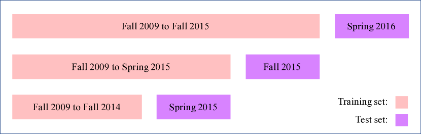
Figure 1: Different Experimental Protocols

5.3 Evaluation Metrics

We use Root Mean Squared Error (RMSE) and Mean Absolute Error (MAE) as metrics for evaluation, and are defined as follows:

$$\begin{split}RMSE=\sqrt{\frac{\sum_{s,c\in G_{T}}(g_{s,c}-\tilde{g}_{s,c})^{2}}{\left|G_{T}\right|}},\\ MAE=\frac{\sum_{s,c\in G_{T}}\left|g_{s,c}-\tilde{g}_{s,c}\right|}{\left|G_{T}\right|}\end{split}$$

where $g_{s,c}$ and $\tilde{g}_{s,c}$ are the ground truth and predicted grade for student $s$ on course $c$, and $G_{T}$ is the testing set of (student, course, grade) triples in the $T_{th}$ term. Normally, in next-term grade prediction problem, MAE is more intuitive than RMSE since MAE is a straightforward method which calculates the deviation of errors directly while RMSE has implications such as penalizing large errors more.

For our dataset, a student’s grade can be a letter grade (i.e. A, A-, …, F). As done previously by Polyzou et. al. [24] we define a tick to denote the difference between two consecutive letter grades (e.g., C+ vs C or C vs C-). To assess the performance of our grade prediction method, we convert the predicted grades into their closest letter grades and compute the percentage of predicted grades with no error (or 0-ticks), within 1-tick and within 2-ticks denoted by Pct₀, Pct₁ and Pct₂, respectively. For the problem of course selection and degree planning, courses predicted within 2 ticks can be considered sufficiently correct. We name these metrics as Percentage of Tick Accuracy (PTA).

5.4 Baseline Methods

We compare the performance of our proposed method to the following baseline approaches.

5.4.1 Matrix Factorization

Matrix factorization is known to be successful in predicting ratings accurately in recommender systems  [26]. This approach can be applied directly on next-term grade prediction problem by considering student-course grade matrix as a user-item rating matrix in recommender systems. Based on the assumption that each course and student can be represented in the same low-dimensional space, corresponding to the knowledge space, two low-rank matrices containing latent factors are learned to represent courses and students  [30]. Specifically, the grade a student $s$ will achieve on a course $c$ is predicted as follows:

$$\begin{aligned} \tilde{g}_{s,c}=\mu+\mathbf{p}_{s}+\mathbf{q}_{c}+\mathbf{u}_{s}^{\mathsf{T}}\mathbf{v}_{c}\end{aligned}$$ (12)

where $\mu$ is a global bias term, $\mathbf{p}_{s}$ ($\mathbf{p}\in\mathbb{R}^{n}$) and $\mathbf{q}_{c}$ ($\mathbf{q}\in\mathbb{R}^{m}$) are the student and course bias terms (in this case, for student $s$ and course $c$), respectively, and $\mathbf{u}_{s}$ ($\mathbf{U}\in\mathbb{R}^{k\times n}$) and $\mathbf{v}_{c}$ ($\mathbf{V}\in\mathbb{R}^{k\times m}$) are the latent factors for student $s$ and course $c$, respectively.

5.4.2 Matrix Factorization without Bias (MF₀)

We only considered the student and course latent factors to predict the next-term grades. Therefore, the grade a student $s$ will achieve on a course $c$ is calculated as follows:

$$\begin{aligned} \tilde{g}_{s,c}=\mathbf{u}_{s}^{\mathsf{T}}\mathbf{v}_{c}\end{aligned}$$ (13)

5.4.3 Non-negative Matrix Factorization (NMF)  [15]

We add non-negative constraints on matrix $\mathbf{U}$ and matrix $\mathbf{V}$ in Equation 13. The non-negativity constraints allows MF approaches to have better interpretability and accuracy for non-negative data [10].

6 Results and Discussion

6.1 Overall Performance

Table 2: Comparison Performance with PTA (%)

Methods	Spring 2016			Fall 2015			Spring 2015
	Pct0($\uparrow$)	Pct1($\uparrow$)	Pct2($\uparrow$)	Pct0	Pct1	Pct2	Pct0	Pct1	Pct2
MF	13.25	27.71	58.02	12.05	26.63	58.89	13.03	26.09	54.83
MF0	16.52	31.65	57.46	15.51	30.03	55.64	15.53	29.53	54.94
NMF	13.21	27.04	57.18	15.33	30.12	56.15	15.56	29.23	54.93
MFTCI	19.78	35.52	61.44	19.71	35.16	60.12	18.56	32.78	58.80

• i) “$\uparrow$" indicates the higher the better. ii) Reported values of Pct₀, Pct₁ and Pct₂ are percentages. iii) Best performing methods are highlighted with bold.

Table 2 presents the comparison of Pct₀, Pct₁ and Pct₂ for non-transfer students for the three terms considered as test: Spring 2016, Fall 2015 and Spring 2015. We observe that the MFTCI model outperforms the baselines across the different test sets. On average, MFTCI outperforms the MF, MF₀ and NMF methods by 34.18%, 11.59% and 4.08% in terms of Pct₀, 16.64%, 7.96% and 4.03% in terms of Pct₁, and 2.10%, 3.00% and 1.98% in terms of Pct₂, respectively. We observe similar results for transfer students as well (not included here for brevity).

Table 3 presents the performance of the baselines and MFTCI model for the three different terms of both non-transfer and transfer students using RMSE and MAE as evaluation metrics. The MFTCI model consistently outperforms the baselines across the different datasets in terms of MAE. In addition, the results shows that MF₀, NMF and MFTCI tend to have better performance for Spring 2016 term than Fall 2015 term. Similar trend is observed between Fall 2015 term and Spring 2015 term. This suggests that MFTCI is likely to have better performance with more information in the training set.

Table 3: Comparison Performance with RMSE and MAE.

Methods	Non-Transfer Students								Transfer Students
	Spring 2016			Fall 2015			Spring 2015		Spring 2016			Fall 2015			Spring 2015
	RMSE	MAE		RMSE	MAE		RMSE	MAE	RMSE	MAE		RMSE	MAE		RMSE	MAE
MF	0.999	0.754		1.037	0.786		1.023	0.784	0.925	0.688		0.921	0.686		0.985	0.732
MF0	0.929	0.714		0.977	0.752		1.014	0.778	0.893	0.668		0.944	0.705		1.011	0.765
NMF	1.020	0.769		0.967	0.746		1.000	0.771	0.906	0.683		0.932	0.701		0.979	0.746
MFTCI	0.928	0.685		0.982	0.717		1.012	0.750	0.887	0.636		0.927	0.662		1.000	0.721

6.2 Analysis on Individual Majors

Table 4: Comparison Performance for Different Majors

	Methods	AIT	BIOL	CEIE	CPE	CS	PSYC
Pct0	MF	18.71	18.00	15.99	12.99	15.98	20.18
	MF0	19.45	22.10	16.70	14.21	16.47	22.12
	NMF	19.77	22.16	17.01	14.32	16.61	22.17
	MFTCI	22.30	24.24	16.80	14.32	17.32	25.83
Pct1	MF	37.95	35.43	31.47	27.86	31.53	39.41
	MF0	37.21	39.68	31.87	27.97	30.51	39.63
	NMF	36.79	39.74	31.67	27.19	30.43	39.36
	MFTCI	39.64	40.87	32.38	27.53	31.78	42.29
Pct2	MF	67.02	67.78	58.66	52.28	56.91	71.01
	MF0	66.17	67.54	58.35	50.72	56.24	67.74
	NMF	66.70	67.54	58.55	51.17	56.17	67.79
	MFTCI	66.70	68.25	58.76	52.94	58.18	68.29

We divide non-transfer students based on their majors and test the baselines and MFTCI model on each major, separately. Table 4 shows the comparison of Pct₀, Pct₁ and Pct₂ on different majors. The results show that MFTCI has the best performance for almost all the majors. Among all the results, MFTCI has the highest accuracy when predicting grades for PSYC and BIOL students for which we have more student-course pairs in the training set.

6.3 Effects from Previous Terms on MFTCI

In order to see the influence of number of previous terms considered in MFTCI, we run our model with only $\Delta(T-1)$ in Equation 1. This method is represented as MFTCI_p1. Figure 2 shows the comparison results of MAE for six subsets of data which are reported in Table 3, where “NTR" stands for non-transfer students and “TR" stands for transfer students. The results show that MFTCI consistently outperforms MFTCI_p1 on all datasets. This suggests that considering two previous terms is necessary for achieving good prediciton results. Moreover, since we consider that the student’s knowledge is modeled using an exponential decaying function over time, we do not include the influence from the third previous term in our model as its influence for the grade prediction is negligible in comparison to the previous two terms.

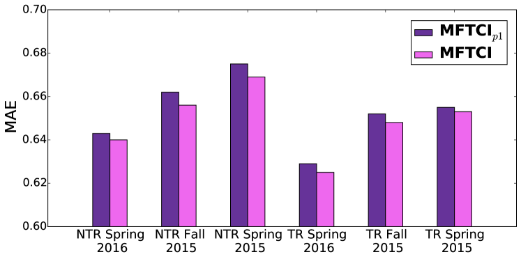
Figure 2: Comparison performance for MFTCI_p1 and MFTCI

6.4 Visualization of Course Influence

Figure 3: Identified course influences for CS major

Figure 4: Identified course influences for AIT major

To interpret what is captured in the course influence matrix $A$ (See Eq 1), we extract the top 20 values with the corresponding course names (and topics) for analysis. Figure 3 and 4 show the captured pairwise course influences for CS and AIT majors, respectively. Each node corresponds to one course which is represented by the shortened course’s name. We can notice from the figures that most influences reflect content dependency between courses. For example, in the CS major, “Object Oriented Programming" course has significant influence on performance of “Low-Level Programming" course (the former one is also the latter one’s prerequisite course); “Linear Algebra" and “Discrete Mathematics" have influence on each other; “Formal Methods & Models" course has influence on “Analysis of Algorithms" course. In case of the AIT major, both “Introductory IT" course and “Introductory Computing" course have influence on “IT Problem & Programming" course; “Multimedia & Web Design" course has influence on both “Applied IT Programming" course and “IT in the Global Economy" course. GMU has a sample schedule of eight-term courses for each major in order to guide undergraduate students to finish their study step by step based on the level, content and difficulty of courses . Among the identified relationships shown in Figures 3 and 4 we found 17 and 13 of the CS and AIT courses influences in the guide map, respectively. The rest of the identified influences are among other general electives but required courses (e.g., “Public Speaking" course), or specific electives pertaining to the major (e.g., “Research Methods” course). This shows that our model learns meaningful course-wise influences and successfully uses it to improve MF model.

Figure 5 shows the identified course influences for the BIOL, CEIE, CPE and PSYC majors. These identified course-wise influences seem to capture similarity of course content.

(a) Identified course influences for BIOL major

(b) Identified course influences for CEIE major

(c) Identified course influences for CPE major

(d) Identified course influences for PSYC major

Figure 5: Identified course influences for different majors

7 Conclusion and Future Work

We presented a Matrix Factorization with Temporal Course-wise Influence (MFTCI) model that integrates factorization models and the influence of courses taken in the preceding terms to predict student grades for the next term.

We evaluate our model on the student educational records from Fall 2009 to Spring 2016 collected from George Mason University. The dataset in this study contains both non-transfer and transfer students from six different majors. Our experimental evaluation shows that MFTCI consistently outperforms the different state-of-the-art methods. Moreover, we analyze the effects from previous terms on MFTCI, and we make the conclusion that it is necessary to consider two previous terms. In addition, we visualize the patterns learned between pairs of courses. The results strongly demonstrate that the learned course influences correlate with the course content within academic programs.

In the future, we will explore incorporation of additional constraints over the the pairwise course influence matrix, such as prerequisite information, compulsory and elective provision of a course. We will explore using the course influence information to build a degree planner for future students.

8 Acknowledgments

Funding was provided by NSF Grant, 1447489.

Appendix A Computational Complexity Analysis

The computational complexity of MFTCI is determined by the four steps in the alternating approach as described above. To update $U$ and $V$ as in Equation 2 using gradient descent method via alternating minimization, the computational complexity is $O(\text{niter}_{uv}(k\times n_{s,c}+k\times m+k\times n))=O(\text{niter}_{uv}(k\times n_{s,c}))$ (typically $n_{s,c}\geq\max(m,n)$), where $n_{s,c}$ is the total number of student-course dyads, $n$ is the number of students, $m$ is the number of courses, $k$ is the latent dimensions of $U$ and $V$, and $\text{niter}_{uv}$ is the number of iterations. To update $A$ as in Equation 3 using gradient descent method, the computational complexity is upper-bounded by $O(\text{niter}_{a}(n_{cc}\times\frac{n_{s,c}}{m}))$, where $n_{cc}$ is the number of course pairs that have been taken by at least one student, $\frac{n_{s,c}}{m}$ is the average number of students for a course, which upper bounds the average number of students who co-take two courses, and $\text{niter}_{a}$ is the number of iteractions. Essentially, to update $A$, we only need to update $A(c_{i},c_{j})$ where $c_{i}$ and $c_{j}$ have been co-taken by some students. For $A(c_{i},c_{j})$ where $c_{i}$ and $c_{j}$ have never been taken together, they will remain 0. To update $Z_{1}$ as in Equation 4, a singular value decomposition is involved and thus its computational complexity is upper bounded by $O(m^{3})$. To update $Z_{2}$ as in Equation 8, the computational complexity is $O(m^{2})$. To update $U_{1}$ and $U_{2}$ as in Equation 11, the computational complexity is $O(m^{2})$. Thus, the computational complexity for MTFCI is $O(\text{niter}(\text{niter}_{uv}(k\times n_{s,c})+\text{niter}_{a}(n_{cc}\times\frac{n_{s,c}}{m})+m^{3}+m^{2}))$ = $O(\text{niter}(\text{niter}_{uv}(k\times n_{s,c})+\text{niter}_{a}(n_{cc}\times\frac{n_{s,c}}{m})+m^{3}))$, where niter is the number of iterations for the four steps. Although the complexity is dominated by $m^{3}$ due to the SVD on $A+U_{1}$, since $n$ (i.e., the number of courses) is typically not large, the run time will be more dominated by $n_{s,c}$ (i.e., the number of student-course dyads).

References

- [1] Charu C. Aggarwal. Recommender Systems: The Textbook. Springer Publishing Company, Incorporated, 1st edition, 2016.
- [2] RSJD Baker et al. Data mining for education. International encyclopedia of education, 7:112–118, 2010.
- [3] Stephen Boyd, Neal Parikh, Eric Chu, Borja Peleato, and Jonathan Eckstein. Distributed optimization and statistical learning via the alternating direction method of multipliers. Foundations and Trends® in Machine Learning, 3(1):1–122, 2011.
- [4] Hana Bydžovská. Are collaborative filtering methods suitable for student performance prediction? In Portuguese Conference on Artificial Intelligence, pages 425–430. Springer, 2015.
- [5] Freddy Chong Tat Chua, Richard J Oentaryo, and Ee-Peng Lim. Modeling temporal adoptions using dynamic matrix factorization. In 2013 IEEE 13th International Conference on Data Mining, pages 91–100. IEEE, 2013.
- [6] Tristan Denley. Course recommendation system and method, January 10 2013. US Patent App. 13/441,063.
- [7] Yi Ding and Xue Li. Time weight collaborative filtering. In Proceedings of the 14th ACM International Conference on Information and Knowledge Management, CIKM ’05, pages 485–492, New York, NY, USA, 2005. ACM.
- [8] Asmaa Elbadrawy, Scott Studham, and George Karypis. Personalized multi-regression models for predicting students performance in course activities. UMN CS, pages 14–011, 2014.
- [9] Wu He. Examining students’ online interaction in a live video streaming environment using data mining and text mining. Computers in Human Behavior, 29(1):90–102, 2013.
- [10] Ngoc-Diep Ho. Nonnegative matrix factorization algorithms and applications. PhD thesis, ÉCOLE POLYTECHNIQUE, 2008.
- [11] Chein-Shung Hwang and Yi-Ching Su. Unified clustering locality preserving matrix factorization for student performance prediction. IAENG Int. J. Comput. Sci, 42(3):245–253, 2015.
- [12] Bin Ju, Yuntao Qian, Minchao Ye, Rong Ni, and Chenxi Zhu. Using dynamic multi-task non-negative matrix factorization to detect the evolution of user preferences in collaborative filtering. PloS one, 10(8):e0135090, 2015.
- [13] Yehuda Koren, Robert Bell, and Chris Volinsky. Matrix factorization techniques for recommender systems. Computer, 42(8):30–37, August 2009.
- [14] Yehuda Koren, Robert Bell, Chris Volinsky, et al. Matrix factorization techniques for recommender systems. Computer, 42(8):30–37, 2009.
- [15] Daniel D Lee and H Sebastian Seung. Algorithms for non-negative matrix factorization. In Advances in neural information processing systems, pages 556–562, 2001.
- [16] Dixin Luo, Hongteng Xu, Yi Zhen, Xia Ning, Hongyuan Zha, Xiaokang Yang, and Wenjun Zhang. Multi-task multi-dimensional hawkes processes for modeling event sequences. In Proceedings of the 24th International Conference on Artificial Intelligence, IJCAI’15, pages 3685–3691. AAAI Press, 2015.
- [17] Rabab Naqvi. Data mining in educational settings. Pakistan Journal of Engineering, Technology & Science, 4(2), 2015.
- [18] Xia Ning, Christian Desrosiers, and George Karypis. A comprehensive survey of neighborhood-based recommendation methods. In Francesco Ricci, Lior Rokach, and Bracha Shapira, editors, Recommender Systems Handbook, pages 37–76. Springer, 2015.
- [19] Michelle Parker. Advising for retention and graduation. 2015.
- [20] Michael J. Pazzani and Daniel Billsus. The adaptive web. chapter Content-based Recommendation Systems, pages 325–341. Springer-Verlag, Berlin, Heidelberg, 2007.
- [21] Alejandro Peña-Ayala. Educational data mining: A survey and a data mining-based analysis of recent works. Expert systems with applications, 41(4):1432–1462, 2014.
- [22] Štefan Pero and Tomáš Horváth. Comparison of collaborative-filtering techniques for small-scale student performance prediction task. In Innovations and Advances in Computing, Informatics, Systems Sciences, Networking and Engineering, pages 111–116. Springer, 2015.
- [23] Agoritsa Polyzou and George Karypis. Grade prediction with models specific to students and courses. International Journal of Data Science and Analytics, pages 1–13, 2016.
- [24] Agoritsa Polyzou and George Karypis. Grade prediction with models specific to students and courses. International Journal of Data Science and Analytics, pages 1–13, 2016.
- [25] Sanjog Ray and Anuj Sharma. A collaborative filtering based approach for recommending elective courses. In International Conference on Information Intelligence, Systems, Technology and Management, pages 330–339. Springer, 2011.
- [26] Francesco Ricci, Lior Rokach, Bracha Shapira, and Paul B Kantor. Recommender systems handbook., 2011.
- [27] Jill M Simons. A National Study of Student Early Alert Models at Four-Year Institutions of Higher Education. ERIC, 2011.
- [28] John Z Sun, Dhruv Parthasarathy, and Kush R Varshney. Collaborative kalman filtering for dynamic matrix factorization. IEEE Transactions on Signal Processing, 62(14):3499–3509, 2014.
- [29] John Z Sun, Kush R Varshney, and Karthik Subbian. Dynamic matrix factorization: A state space approach. In 2012 IEEE International Conference on Acoustics, Speech and Signal Processing (ICASSP), pages 1897–1900. IEEE, 2012.
- [30] Mack Sweeney, Jaime Lester, and Huzefa Rangwala. Next-term student grade prediction. In Big Data (Big Data), 2015 IEEE International Conference on, pages 970–975. IEEE, 2015.
- [31] Mack Sweeney, Huzefa Rangwala, Jaime Lester, and Aditya Johri. Next-term student performance prediction: A recommender systems approach. arXiv preprint arXiv:1604.01840, 2016.
- [32] Nguyen Thai-Nghe, Lucas Drumond, Artus Krohn-Grimberghe, and Lars Schmidt-Thieme. Recommender system for predicting student performance. Procedia Computer Science, 1(2):2811–2819, 2010.
- [33] Liang Xiong, Xi Chen, Tzu-Kuo Huang, Jeff Schneider, and Jaime G. Carbonell. Temporal Collaborative Filtering with Bayesian Probabilistic Tensor Factorization, pages 211–222. 2010.
- [34] Chenyi Zhang, Ke Wang, Hongkun Yu, Jianling Sun, and Ee-Peng Lim. Latent factor transition for dynamic collaborative filtering. In SDM, pages 452–460. SIAM, 2014.