Robust estimation in single index models when the errors have a unimodal density with unknown nuisance parameter
Abstract
In this paper, we propose a robust profile estimation method for the parametric and nonparametric components of a single index model when the errors have a strongly unimodal density with unknown nuisance parameter. Under regularity conditions, we derive consistency results for the link function estimators as well as consistency and asymptotic distribution results for the single index parameter estimators. Under a log–Gamma model, the sensitivity to anomalous observations is studied by means of the empirical influence curve. We also discuss a robust fold procedure to select the smoothing parameters involved. A numerical study is conducted to evaluate the small sample performance of the robust proposal with that of their classical relatives, both for errors following a log–Gamma model and for contaminated schemes. The numerical experiment shows the good robustness properties of the proposed estimators and the advantages of considering a robust approach instead of the classical one.
1 Introduction
Semiparametric models are an appealing compromise between parametric and nonparametric paradigms. These models represent an intermediate point between a fully parametric model, which is usually of easy interpretation but vulnerable to poor specification, and a fully nonparametric model, which is more flexible but suffers from the well–known curse of dimensionality. Semiparametric modeling combines parametric components with nonparametric ones, retaining the advantages of both types of approaches and avoiding their drawbacks.
Single index models are a relevant topic within the broad class of semiparametric methods with a great potentiality when modelling data in different scientific disciplines. These models have raised a lot of interest in part due to the fact that they reduce the dimensionality of the covariates through a suitable projection linked to the parametric component, while at the same time they capture a possible nonlinear relationship through an unknown smooth function.
Under a single index model, the response variable is related to the covariates through the equation
| (1) |
where the single index parameter and the link univariate real valued function are both unknown. For the sake of identifiability, it is assumed with no loss of generality that and the last component of is positive, where denotes the Euclidean norm. Furthermore, in the classical setting, it is usually assumed that and .
As noted above, in our framework , so we may assume that , without loss of generality. However, some authors consider a different parametrization given by
| (2) |
where with and , which also leads to an identifiable model. One of the advantages of the parametrization (1) over that given in (2) is that the finite dimensional parameter naturally belongs to a compact set. The relation between both parametrizations is given by and , while and . So, estimators in any of these two parametrizations lead to estimators in the other one.
Single index models have received an increasing amount of attention in the last years, probably because they have an appealing feature: they cope with the curse of dimensionality combining nonparametric and parametric–driven approaches. Beneath single index models underlies the idea that the contribution of the vector of covariates to the response can be expressed in terms of a one–dimensional projection. In this sense, these models can be seen as a dimension reduction technique since, once has been estimated, the unidimensional variable can be used as a univariate carrier to estimate nonparametrically the function .
There is an extensive literature in this area. Among the first works, we can mention Powell et al. (1989), Härdle and Stoker (1989), Härdle et al. (1993), Xia et al. (2002) and Carroll et al. (1997). More recently, Xia (2006) studies the asymptotic distribution of two classes of estimators, Chang et al. (2010) consider the heteroscedastic case and Xia et al. (2012) propose a family of estimators of the nonparametric component for which it is not necessary to undersmooth in order to obtain a rate estimator of the parametric component. On the other hand, Wu et al. (2010) consider the estimation of the single index quantile regression, while Liu et al. (2013) propose robust estimators by means of the mode, without taking into account the estimation of a possible scale factor. Xue and Zhu (2006) focus on the problem of looking for confidence regions and intervals and Zhang et al. (2010) study the problem of testing hypotheses that involve . Recently, Li and Patilea (2017) considered a a quadratic form criterion involving kernel smoothing and propose a resampling method to build confidence intervals for the index parameter. Wang et al. (2014) also consider the extension of these models to the situation in which there are missing responses. All the aforementioned procedures are based on classical methods and hence, they are very sensitive to the presence of outliers.
Indeed, even when different approaches have been proposed for fitting model (1), such as kernel smoothing or sliced inverse regression methods, in most cases it is assumed that the error distribution has finite first moment. In the robust framework, this assumption is generally replaced by the symmetry of the error term distribution, in order to achieve Fisher–consistent estimators. However, in practice, situations arise in which the errors are asymmetric, as it is the case when the error term distribution belongs to some class of exponential families, such as the log–Gamma distribution. In this paper, we focus on the problem of robust estimating the parametric and nonparametric components of model (1) when the density of the error is of the form
| (3) |
where is an unknown parameter and is a continuous function with unique mode at . An appealing feature of this family of distributions is that enables to model either symmetric or asymmetric errors, as well. A prominent member of this family is the log–Gamma distribution that is frequently used to fit asymmetric data.
A first approach to deal with outliers in the responses, was given in Delecroix et al. (2006) who considered type estimators for single index models with known nuisance parameter. However, in most cases, the nuisance parameter is unknown and its estimation is crucial to down–weight large residuals. In fact, as in linear regression, it is necessary to determine the size of the residuals to decide if an observation is an outlier or not and this task strongly depends on a good preliminary nuisance parameter estimator. Indeed, the most popular example of model (1) with errors having a density given by (3) is the usual regression model with symmetric errors , where stands for the scale parameter. In this setting, the nuisance parameter is usually taken as to avoid an assumption on a fixed given errors distribution. On the other hand, as mentioned, a well–known regression model with asymmetric errors is the log–Gamma model which corresponds to the Generalized Linear Model for the Gamma distribution with link function. In this case, represents the shape parameter. In both regression models, it is important to estimate in order to calibrate the robust estimators. For this reason, our approach includes a nuisance parameter which needs to be robustly estimated prior to the estimation of and and which may be or a known function of it such as the constant needed to calibrate the estimators.
The aim of this paper is to propose a class of robust estimators for single index models when the errors distribution has density satisfying (3) with the parameter unknown. For this purpose, we introduce a stepwise procedure based on robust profile estimators. We make special emphasis in the case of errors with log–Gamma distribution, which is often employed in applications, and then we extend the proposal to the general setting. Under mild conditions, the estimators of are consistent and the parametric component estimators are consistent and asymptotically normal with rate. We also provide a class of initial estimators and a robust fold procedure to select the bandwidth parameters involved in our proposal.
The outline of the paper is as follows. In Section 2, the three–step procedure for robust estimation under a single index model is introduced first for log–Gamma errors and then, it is extended to more general situations. In Section 3, we give some asymptotic properties of the proposal, while in Section 4, we compute the empirical influence function which may be helpful to study the sensitivity of the estimators to atypical observations. Section 5 presents a robust fold cross–validation method to select the smoothing parameters. The robustness and performance for finite samples of the proposed method are studied by means of a numerical study in Section 6. Proofs are relegated to the Appendix.
2 The estimators
Let be independent observations that follow model (1) for and and assume that the errors are independent, independent of and have density (3) with . Denote the expectation under the true model and the true nuisance parameter which as mentioned above is a function of .
2.1 The log–Gamma setting
In order to introduce the proposed estimators, let us first revisit the particular case of the purely parametric regression model with log–Gamma errors, that is, with density
| (4) |
Assume that the variable and the covariates are such that , where the parametrization is such that and . Hence, defining , we have that and therefore, if and , we get that
| (5) |
where has a density given by (4) with , i.e., it belongs to the family given in (3).
In the log–Gamma model, the classical estimators are based on the maximum likelihood method and are defined through the minimization of the deviance, whose components are given by . A natural way to robustify these estimators is by means of an estimation procedure. Thus, if , , are independent observations following model (5), an estimator is defined as
| (6) |
where is a preliminary estimate of a tuning constant and is a bounded and continuous loss function such as the Tukey’s biweight function given by . For this family of distributions, the nuisance parameter can be taken as the tuning constant that is related to the unknown shape parameter . Fisher–consistency for this family of estimators has been studied in Bianco et al. (2005), under general conditions.
With this background in mind, let us now consider the case of a single index model with log–Gamma errors, that is, , , is a random sample where
| (7) |
We will borrow some of the previous ideas to introduce a robust profile method that involves smoothing and parametric techniques. Profile likelihood procedures were studied by van der Vaart (1988) and applied to generalized partially linear models by Severini and Wong (1992) and Severini and Staniswalis (1994). In order to introduce the smoothers, we will consider local weights. For the sake of simplicity, given we define the kernel weights as
where with a kernel function, i.e., a nonnegative integrable function on and is the bandwidth parameter. The weights depend on the closeness between the point and the projection of on the direction , i.e., between and . To assume that a consistent estimator of the tuning constant, , is available, let stand for a preliminary robust consistent estimator of allowing to define . The latter estimators must be properly computed according to the underlying errors distribution whose density we assume in the family given in (3). In Section 2.3, we introduce a robust consistent estimator of the nuisance parameter for the usual regression model with symmetric errors and for the log–Gamma regression model, as well.
Then, for the particular situation of model (7) we propose the following stepwise procedure
- Step LG1:
-
For each fixed , with , let
- Step LG2:
-
Define the estimators of as the minimum of among , where
and is a weight function.
- Step LG3:
-
Define the final estimator of as with
The robust estimators are obtained controlling large values of the deviance with a bounded loss function . A popular choice is the Tukey’s bisquare loss function , while estimates the tuning constant selected to attain a given efficiency. As mentioned above, depends on the shape parameter (see Bianco et al., 2005). Note that the three steps involve the function
where, as above, .
2.2 The proposal for the general setting (3)
Let us now consider the general case in which the errors have a density in the family (3). In order to extend the proposal given in Section 2.1 to this situation, one may consider a loss function bounding the deviances. To be more precise, let us denote as
where , with the unique mode of the density and is the tuning constant related to the nuisance parameter. As in Maronna et al. (2006), is a function, that is, an even function, non–decreasing on , increasing for when and such that .
We define for each and any continuous function the functions
| (8) | |||||
| (9) |
where is a weight function as above. Denote as . Note that since we are considering the deviance and a continuous family of distributions with strongly unimodal density, there is no need to introduce a correction term to attain Fisher–consistency (see Bianco et al., 2005). More precisely, we have that and , furthermore is the unique minimum of .
In order to define consistent estimators of the parametric and nonparametric components, let us consider the empirical versions of the objective functions (8) and (9), respectively, as
where is any continuous function .
Assume that an initial robust estimator of , , is available. For a general single index model, the robustified profile method can thus be defined as
- Step 1:
-
For each fixed , with , let
- Step 2:
-
Define the estimators of as
- Step 3:
-
Define the final estimator of as with
Note that the stepwise procedure defined by Step LG.1–Step LG.3 corresponds to Step 1–Step 3 for a particular choice of the function .
It is worth noticing that this stepwise procedure only involves unidimensional nonparametric smoothers, preventing from the sparsity of the data induced by the dimensionality of the covariates. In the third step a local polynomial of first degree is computed in order to improve the estimation of the link function . When nuisance parameters are present, they may be estimated using a preliminary estimator which will allow to define also the tuning constant as motivated in the next section.
2.3 Initial estimators
The calibration of the robust estimators will need the computation of a preliminary estimator of the nuisance parameter . As described in the Introduction, as for many robust estimators, this is a crucial issue for the three-step procedure and it can be accomplished in different ways according to the underlying error distribution. We will illustrate the computation of an initial estimator of the nuisance parameter for the log-Gamma model, which can be extended to the case of errors with density in the family given in (3). In Section 2.4 we consider the situation in which the errors have a symmetric distribution.
The preliminary estimator of the shape parameter under model (7) allows to compute the tuning constant by means of an estimator. estimators were introduced by Rousseeuw and Yohai (1984) for ordinary regression and studied in the framework of linear regression with asymmetric errors in Bianco et al. (2005). Let be the bisquare function and consider the following estimator.
- Step ILG.1
-
For each value of , and , compute as the solution of
where, for instance, and . Define as the value
- Step ILG.2
-
For each , let be the solution of
Now, the estimator of is given by and .
- Step ILG.3
This method provides an estimator of as well as an initial estimator of , which is robust, but may be inefficient. It also provides an estimator of the function as . These estimators may be used to start the stepwise estimation procedure in Steps LG1 to LG3 given above. In Bianco et al. (2005) it is shown that is a one–to–one function and thus invertible. For this reason, they recommend to take .
It is worth noting that if we replace by in the initial Steps ILG.1 to ILG.3, the described procedure provides preliminary estimators when the errors have density given by (3).
2.4 The model with symmetric errors
As it is noted above, the family of densities given in (3) also includes symmetric distributions. In this case, a suitable initial method that exploits this feature of the errors distribution can be introduced. Thus, as a second example, we consider the symmetric setting. We set and , where is the tuning constant needed to obtain a scale Fisher–consistent estimator. For instance, when dealing with Tukey’s bisquare function , the choice and leads to a scale estimator Fisher–consistent at the normal distribution with breakdown point 50%. Then, to provide a preliminary estimator of the true scale parameter , let us consider an estimator that can easily be computed as follows.
- Step IS.1
-
For each value of and , compute as the median of the empirical local distribution
- Step IS.2
-
For each , let be the solution of
where, for instance, . Now, the estimators of and are given as and .
To improve the efficiency of the estimators of , consider , with , and define an procedure as follows.
- Step S.1
-
For each value of and , compute as
- Step S.2
-
Define the estimator as
- Step S.3
-
For each value of , define the final estimator of as with
Note that the stepwise procedure defined by Steps S.1 to S.3 corresponds to Step 1–Step 3 for a particular choice of the function , that is, .
3 Asymptotic results
In this section, we derive, under some regularity conditions, the consistency of the estimators defined in Section 2.2 through Steps 1 to 3. We will assume that . Let be a compact set and define the set , where is the unit ball in , i.e., . For any continuous function denote . We consider the following set of assumptions:
-
A1.
The loss function and the function defined in (3) are continuous. Moreover, and are bounded.
-
A2.
The kernel is an even, nonnegative, continuous and bounded function, with bounded variation, satisfying , and as .
-
A3.
The bandwidth sequence is such that , when .
-
A4.
i) The marginal density of is bounded in .
ii) Given any compact set , there exists a positive constant such that for all and , where is the marginal density of . -
A5.
The function satisfies the following equicontinuity condition: given and compact sets, for any there exists such that for any ; and ,
-
A6.
The function is continuous and is a continuous function on .
-
A7.
The initial estimator of , , is a consistent estimator.
-
A8.
The functions and are differentiable functions.
Remark 1. Condition A1 is fulfilled by the loss functions commonly used in the framework of robustness such as Tukey’s bisquare function and guarantees that is a continuous and bounded function. Assumptions A2 and A3 are standard in nonparametric regression. Moreover, A2 is verified for the Epanechnikov and Gaussian kernels, while A3 is satisfied choosing for . A4 is a standard condition in semiparametric models; in particular ii) is achieved if for any . Note that A8 entails that is a continuously differentiable function with respect to . We will denote as its partial derivative with respect to .
The following Lemma gives the uniform convergence of to . Its proof is omitted since it follows using analogous arguments to those considered in the proof of Lemma 3.1 in Boente and Rodriguez (2012).
Lemma 1. Let and be compact sets and assume that there exists such that , where stands for the closure of a -neighbourhood of . Assume that A1 to A6 hold and that the family of functions has a covering number satisfying , for any and some positive constants and , where stands for any probability measure for . Then, we have that
-
a)
.
-
b)
If , then , where .
Remark 2. The condition on the infimum assumed in Lemma 1b) warranties that the infimum of function in (8) is not attained at infinity. Recall that finite–dimensional families of functions are VC–classes of functions as defined in Pollard (1984). Hence, using that
we obtain that the required condition on the covering number depends on the behaviour of the function . In particular, for the log–Gamma regression model, this condition is satisfied for any function.
From Lemma 1, the continuity of as a function of and A7, we obtain the following result recalling that has a unique minimum at .
Theorem 1. Let be defined , where satisfies
| (10) |
Assume that A1 and A8 hold and that . Then, we have that
-
a)
for any compact set .
-
b)
.
The asymptotic distribution of can be derived using the consistency of . In fact, similar arguments to those considered in the proof of Theorem 3.5.3 in Rodriguez (2007) can be used, but taking into account the fact that the estimator of the nuisance parameter is consistent. In particular, we consider below the case of a log–Gamma model.
From now on, we assume that is twice continuously differentiable with first and second derivatives and respectively and that is continuously differentiable in .
Recall that under a log–Gamma model, with independent of , so and . If we define , we have that . Let
| (11) | |||||
| (12) |
Hence, and , where
Define , where
| (13) |
Due to the independence between the errors and the covariates, can be written as
| (14) |
where . Furthermore, consider the matrix
| (15) |
with . Let , , and be the left superior matrices of dimension of , , and , respectively. Assume that is non–singular, , are random vectors with distribution with compact support and the bandwidth satisfies and . Then, using analogous arguments to those considered in Rodriguez (2007) for the case of fixed nuisance parameter and taking into account that , we obtain that
| (16) | |||||
| (17) |
where for any , .
Hence, using (14) and (15), we get that
Since the classical estimator of the single index parameter corresponds to the choice , its asymptotic covariance matrix is of the form , therefore, the asymptotic efficiency with respect to the classical estimator is given by
which equals the efficiency of the regression estimator described in Bianco et al. (2005).
4 Empirical Influence Curve
In this section, we derive the empirical influence function of the single index parameter estimator under a log–Gamma model. The empirical influence function (), introduced by Tukey (1977), measures the robustness of an estimator with respect to a single outlier. Essentially, it assesses the impact on an estimator of adding an arbitrary observation to the sample. Diagnostic measures with the purpose of outlier identification can be defined from the empirical influence functions. Mallows (1974) defines a finite version of the influence function, introduced by Hampel (1974), that is computed at the sample empirical distribution. The has been widely used in parametric statistics, but has retrieved less attention in nonparametric literature. Foremost, Manchester (1996) introduces a simple graphical procedure to display the sensitivity of a scatter plot smoother to perturbations in the data. Tamine (2002) defines a smoothed influence function in the context of nonparametric regression with a fixed bandwidth that is based on Aït Sahalia (1995) smoothed functional approach to nonparametric kernel estimators.
Following Boente and Rodriguez (2010), we consider an empirical influence function that is close to Manchester (1996) approach and at the same time, retains the spirit of the definition introduced by Mallows (1974).
To be more precise, denote the single index parameter estimator based on the original data set . If is the empirical measure that gives weight to each datum in the sample, we have that . Let be the empirical measure that gives mass to each and mass to the arbitrary observation . In other words, we have a new sample with the original data set accounting an proportion and the new observation an proportion. Now, denote the single index parameter estimator for the new sample. We compute the empirical influence function of at a given point as
It is easy to see that the single index estimator is equivariant under orthogonal transformations. Hence, without loss of generality, we can assume that , the th canonical vector of . To obtain the empirical influence function, we will assume that the matrix given in (14) is non–singular, as required when deriving the asymptotic distribution of in Section 3. Furthermore, for simplicity, we will assume that the tuning parameter is fixed.
To avoid burden notation, denote , , and . Moreover, from now on, given , stands for the vector of its first elements. Besides, given the kernel and its first derivative , we define .
Let us assume that is three times continuously differentiable. As in (11) and (12), and stand for the derivatives with respect to of and , respectively, and we further define
Then, if stands for the second order derivative of , we have that with
It is worth noticing that if is three times continuously differentiable and the kernel is continuously differentiable, we have that defined in Step LG1 is continuous and has continuous partial derivatives with respect to and .
Proposition 1. Assume that is three times continuously differentiable, the kernel is continuously differentiable and that , the left superior matrix of dimension of the matrix given in (14) is non–singular. Denote as
| (18) | |||||
| (19) | |||||
where and are estimates of the quantities given in (13), that is,
and
Then, if , the left upper submatrix of , is invertible, we have that
-
a)
and .
-
b)
the empirical influence functions at , , and are given by
where
and
Remark 3. In Proposition 1, the left upper submatrix is assumed to be non–singular. Using the conditional Fisher–consistency, that is, , we have that
under mild conditions, while
Therefore, which implies that . Hence, taking into account that we have assumed that is invertible, we get that with probability converging to 1 is non–singular.
It is worth noticing that even when considering a bounded loss function, such as the Tukey’s bisquare function, the empirical influence function may not be bounded in directions orthogonal to , since the term involving in may not be bounded, unless the function controls large values of the covariates. This behaviour is similar to that arising with projection–pursuit estimators when estimating the principal directions (see Croux and Ruiz–Gazen, 2005).
5 Selection of the smoothing parameters
The estimation of the nonparametric component of the model involves a smoothing parameter both in the first and third steps. Each step may require a different degree of smoothness and for this reason, the bandwidths may be chosen different. The effect of the bandwidth is crucial on the performance of the nonparametric estimator; the smoothing parameter must warranty a balance between bias and variance. The problem of bandwidth selection has been widely studied in nonparametric and semiparametric models and leave-one-out cross validation procedures have been extensively used for this purpose. –fold–cross validation criteria are also a reasonable choice with a computationally cheaper cost.
However, it is well known that classical cross–validation criteria are very sensitive to outliers. It is worth noticing that robust criteria for the selection of the smoothing parameter are needed even when robust estimators are considered. Leung et al. (1993), Wang and Scott (1994), Boente et al. (1997), Cantoni and Ronchetti (2001) and Leung (2005) discuss these ideas in the fully nonparametric framework, while Bianco and Boente (2007) and Boente and Rodriguez (2008) consider robust cross–validation in semiparametric models.
For the initial and final smoothing steps performed in Steps 1 and 3 of the proposed method, we consider a robust version of the classical –fold cross–validation criterion based on the deviance to select the bandwidths. More precisely, let us first randomly split the data set into subsets of similar size, disjoint and exhaustive, with indexes , , such that . Let be the set of bandwidths to be considered in the first step of the proposed procedure. Denote the robust regression estimator computed in Step 2 without the observations with indexes in the set and using as smoothing parameter in the previous step and let be the corresponding nonparametric robust estimator computed in Step 1.
Taking into account that for each , , there exists , , such that , we define the prediction of observation as . Noticing that in the actual setting, the deviance residuals are a suitable measure of the discrepancy between an observation and its predictor, the robust th fold cross–validation smoothing parameter is defined as , where
| (20) |
for a given tuning constant . Denote the robust estimator based on the whole sample when the smoothing parameter is the optimal .
It is worth noticing that the robust th fold cross–validation given in (20) is a robustified version of its classical counterpart that seeks for the smoothing parameter minimizing
| (21) |
where are based on the classical estimators.
In order to select the second bandwidth to be used in the local linear nonparametric estimator described in Step 3, we consider a similar procedure. That is, we take the set of bandwidths to be considered in the third step and denote the robust nonparametric estimator without the observations with indexes in the set and using as smoothing parameter and . Again, reasoning as above, for each , we define the predictor of observation as and so, the robust th fold cross–validation linear smoothing parameter is defined as . Once the data driven–bandwidth is obtained, the final nonparametric estimator denoted can be computed as in Step 3 from the whole sample using this bandwidth.
6 Numerical results
In this Section, we summarize the results of a simulation study designed to compare the performance of the proposed estimators with the classical ones under a log–Gamma model.
We have performed replications with samples of size . For the clean samples the covariates are generated as , while the response variables follow the log–Gamma single–index model , with , and .
In all Tables, the results for the uncontaminated samples are denoted as . Furthermore, the robust estimators introduced in this paper are subindicated with r, while their classical counterparts based on the deviance are subindicated with cl. To be more precise, the robust estimators correspond to those controlling large values of the deviance. In this case, the robust estimators were computed using the Tukey’s bisquare loss function with adaptive tuning constants computed as in Bianco et al. (2005). On the other hand, the classical estimators correspond to choose the loss function equal to the deviance. With respect to the weight or trimming function, in order to make a fair comparison between the classical and robust estimators, we choose , with and for both estimators. The value is selected as in Sherman (1994) to avoid the density of to be too small.
The smoothing parameters were selected as described in Section 5 using a -fold cross–validation procedure. For the classical estimators we use the criterion (21) in each step, while for the robust estimates, we used the robust fold method (20) with that under the central model corresponds to an asymptotic efficiency of 0.90. In all these cases, the set of candidates for the initial bandwidth was taken as an equidistant grid of length 13 between 0.05 and 0.35, while for the local linear smoothing parameter we choose as an equidistant grid of length 25 between 0.05 and 0.35. To simplify the notation, henceforth we denote and the robust estimators computed with the two robust cross–validation bandwidths, while and stand for the classical estimators computed with the bandwidths obtained minimizing (21).
To evaluate the performance of each estimator we compute different measures. For the parametric component, given an estimator of the true single index parameter , we consider as the mean values over replications of . For the nonparametric component, we compute as the mean over replications of and also as the median over replications of , where is a given estimator of the function .
In order to assess the behaviour of the estimators under contamination, we have considered two types of contaminations and samples generated from them. The first set of contaminations introduces moderate outlying points, while with the second one we expect a more dramatic effect on the classical estimators.
Three different models, labelled , and in all Tables and Figures are considered in the moderate contamination scheme. To obtain the contaminated samples, we have first generated a sample for and then, we introduce large values on the responses as
| (22) |
where , with , where is the unit vector orthogonal to the true single index parameter and and under , and , respectively.
The second scheme accounts for more severe contaminations, labelled , and in all Tables and Figures and we guess that its effect on the classical estimators would be more dramatic. To obtain the contaminated samples, the observations are generated as in (22) where now where as above but or , respectively. Figure 1 illustrates the considered contaminations in a generated sample.


Table 1 summarizes the results along the replications. The reported results show the great stability of the robust procedure against moderate and severe contaminations. As expected, when there is no contamination the classical estimators achieve the lowest square errors for both the parametric and nonparametric components. Nevertheless, the performance of the robust estimators is very satisfactory under since the loss of efficiency is very small. Focusing on the parametric component, under any of the contaminated schemes, the performance of the classical estimator is very poor. Table 1 exhibits that the mean square error of the single index parameter increases more than forty times under the moderate contaminations and more than times under the severe ones, while the robust estimator remains very stable in all considered scenarios.
| 0.005 | 0.005 | 0.041 | 0.046 | 0.020 | 0.021 | |
|---|---|---|---|---|---|---|
| 0.209 | 0.008 | 0.294 | 0.061 | 0.164 | 0.031 | |
| 0.357 | 0.007 | 0.408 | 0.060 | 0.226 | 0.030 | |
| 0.534 | 0.007 | 0.521 | 0.058 | 0.287 | 0.028 | |
| 1.064 | 0.013 | 5.393 | 0.059 | 4.510 | 0.024 | |
| 1.098 | 0.008 | 13.282 | 0.057 | 13.282 | 0.023 | |
| 1.106 | 0.006 | 18.057 | 0.053 | 17.436 | 0.022 | |
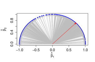
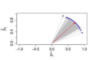
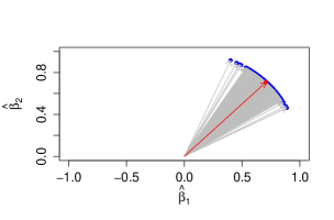
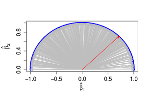
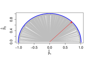
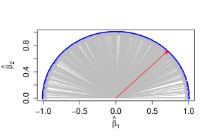
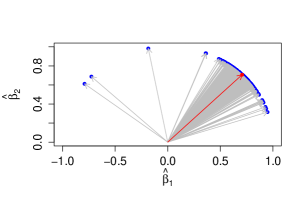
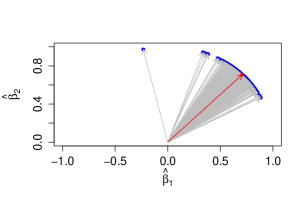
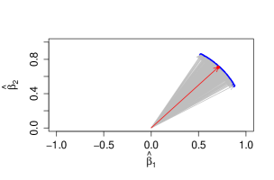
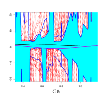
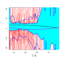
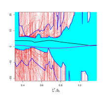
Since an important goal in this framework is to capture the direction of the single index parameter , instead of presenting the traditional boxplots of the estimates, in Figures 2 to 4 we present a two dimensional graph that reflects the skill of the classical and robust estimators to get the true direction , for the clean and contaminated samples. In these plots, the red arrow represents the true direction , that corresponds to an angle and the grey ones to the estimated directions. These figures show that under the performance of the robust estimator of the parametric component is similar to that of the classical estimator since the robust estimates are more or less spread as the classical estimator around the target direction. It also becomes evident that in contaminated samples the robust estimator of the parametric component is very stable under all the contaminated scenarios, while the classical estimator is completely spoiled. Indeed, under to , the classical estimates of the single index parameter tend to be concentrated not only on directions close to the true value but also to its orthogonal direction , showing the impact of the contaminated points. On the other hand, under the severe contaminations to the classical estimates cover almost all possible directions in the first and second quadrants, becoming completely unreliable.
Classical Method Robust Method
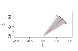
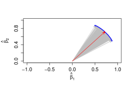
Classical Method
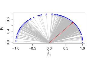
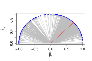
Robust Method

Classical Method
Robust Method
Regarding the estimation of the nonparametric component, Table 1 shows the large effect of the considered contaminations on the classical estimator of the nonparametric component, where the mean square error increases at least seven times under the moderate contaminations. Under the severe contaminations to , the effect of the outliers on the classical estimator is devastating, while it is quite harmless for the robust estimator. It is worth noticing that under all the contamination schemes, the reported values of for the classical estimator, which is a more resistant measure based on the median, are very close to the corresponding values of , making evident that in most replications the classical estimator of the nonparametric component is completely spoiled.
Classical Method Robust Method
Classical Method
Robust Method
Classical Method
Robust Method
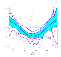
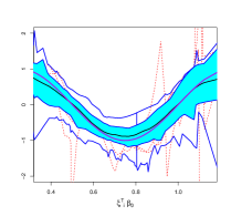
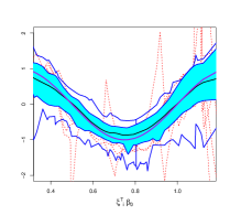
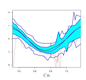
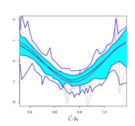
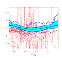
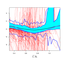
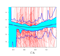
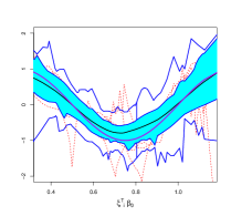
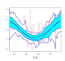
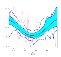
In order to give a full picture of the performance of both classical and robust estimators of , Figures 5 to 7 display their functional boxplots. Since the covariate is random, in order to obtain comparable estimations for , we consider a fixed grid of points , in . Thus, for each replication, we estimate using the classical and robust procedures. In the functional boxplots, the area in light blue represents the central region, the dotted red lines correspond to outlying curves, the black line indicates the deepest curve, while the purple line is the true nonparametric function . It is worth noticing that, for the contaminated settings, due to the effect of the outliers, some curves are out of range when using the classical procedure. For that reason, the functional boxplots of the classical estimators are plotted in a reduced range to allow a clear visualization of the central area. Figure 5 shows that the classical and robust nonparametric estimators of are quite similar under , while Figures 6 to 7 exhibit the devastating effect of the contaminating points, even the moderate ones, on the classical estimator. The impact of the contaminations on the classical estimates is reflected either in the presence of a great number of outlying curves and also in the enlargement of the width of the bars of the functional boxplots. With respect to the robust estimates, despite the fact that a few outlying curves appear, the range of variation of the curves is almost the same than under , the central region in light blue of all the boxplots always contain the true function and most curves follow the pattern introduced by the sine function. In general terms, the functional boxplots show the stability of the robust estimates of which are reliable under the contaminated scenarios as well as the strong effect of the considered contaminations on the classical estimators of the nonparametric component.
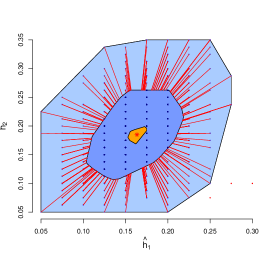
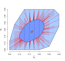
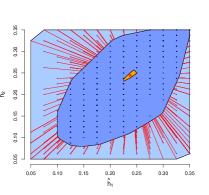
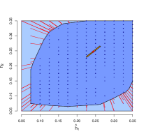
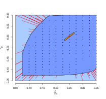
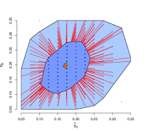
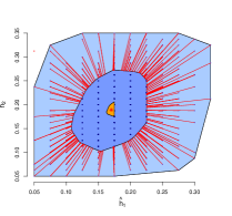
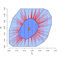
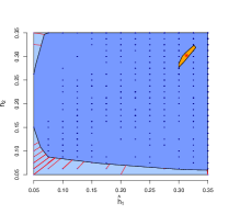
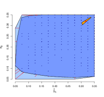
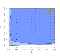
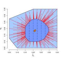
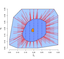
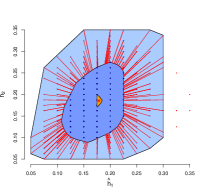
A careful study of the bandwidth behaviour is beyond the scope of the paper, however in order to have a deeper insight of the performance of the selectors under and the considered contaminations, we give a brief analysis of the data–driven parameters obtained in this numerical experiment. Table 2 reports, for both estimators, the median over replications of the cross-validation data–driven bandwidths to be used in Steps 1 and 3 denoted and respectively. On the other hand, in Figures 8 to 10 we present the bagplots corresponding to and selected through the classical and robust cross–validation criteria. Under both criteria lead to similar data–driven smoothing parameters. However, the lack of robustness of the classical cross–validation criterion under contaminations becomes evident from these plots. The classical cross–validation criterion under contaminations tends to choose greater bandwidths and this becomes evident, for instance, from the behaviour of their medians reported in Table 2. The poor behaviour of the classical data–driven bandwidths leads towards over–smoothing which may explain the results reported in Table 1. On the other hand, except for a few cases, the selected bandwidths obtained with the robust criterion remain stable in all circumstances.
| Method | ||||||||
|---|---|---|---|---|---|---|---|---|
| Classical | 0.175 | 0.225 | 0.250 | 0.250 | 0.325 | 0.325 | 0.325 | |
| 0.175 | 0.238 | 0.250 | 0.250 | 0.350 | 0.300 | 0.338 | ||
| Robust | 0.175 | 0.175 | 0.175 | 0.175 | 0.175 | 0.200 | 0.200 | |
| 0.188 | 0.188 | 0.188 | 0.188 | 0.188 | 0.188 | 0.188 |
Classical Method Robust Method
Classical Method
Robust Method
Classical Method
Robust Method
A Appendix
A.1 Proof of Theorem 1.
a) For any , let be a compact set such that . Then, we have that
and so, using (10), the fact that and the Strong Law of Large Numbers, we get that
Therefore, it remains to show that . Define the following class of functions . Using Theorem 3 from Chapter 2 in Pollard (1984), the compactness of , A1, the continuity of given in A6 and analogous arguments to those considered in Lemma 1 from Bianco and Boente (2002), we get that and a) follows.
b) Let be a subsequence of such that , where lies in the compact set . Let us assume, without loss of generality, that . Then, A7, the continuity of , the consistency of and a) entail that and , since . Now, using that and has a unique minimum at , we conclude the proof.
A.2 Proof of Proposition 1.
a) The single index parameter estimation related to Step LG2 is obtained by means of the minimization with respect to of
among the vectors of length one, where, at the same time, is defined as
Hence, if we denote , we have that where is the solution of
Then, satisfies
where
as defined in (11), stands for the derivative of and are given by
Using that , we get that the estimator verifies
and is the solution of
| (A.1) |
Then, if we call
we get that, for any , satisfies Therefore, differentiating with respect to and evaluating at and using that , we obtain that
| (A.2) | |||||
Henceforth, in order to compute and to simplify the presentation, we consider the following functions:
and their corresponding derivatives with respect to
Thus, we have that
Since , we obtain that
| (A.3) | |||||
It remains to compute the functions , and . Straightforward arguments lead to
where . Then, we get that
Analogously, we have that
so
Finally, in a similar way, we obtain that
which implies that
Using the previous expressions, we deduce that
Now, replacing in (A.3) , and with the obtained expression, we have that
Recall that
Then, we get that
where and are defined in (18) and (19). Replacing in (A.2), we have that
It is worth noticing that since , differentiating with respect to and evaluating at , we have that
which, taking into account that , implies that . Therefore, we only have to compute for .
Using again that , we obtain that
Hence, we have that the left superior matrix of equals the matrix , so that implies
| (A.4) |
Therefore, from (A.4) we get that .
It is worth noticing that and involve , and .
b) Let us derive . Since is the solution of (A.1), we have that
Differentiating with respect to and evaluating at , we obtain that
| (A.5) |
Analogously, differentiating first with respect to on both sides of equation (A.1) and then, with respect to and evaluating at , we can obtain an expression for . Alternatively, we may differentiate (A.5) with respect to to obtain
Similar arguments lead to the expression for .
Finally, note that , satisfies
| (A.6) |
Hence, differentiating with respect to equation (A.6), we get that
which implies that
On the other hand, differentiating (A.6) with respect to , we obtain that
which entails that
Acknowledgements. This research was partially supported by Grants pict 2014-0351 from anpcyt and Grant 20120130100279BA from the Universidad de Buenos Aires at Buenos Aires, Argentina. It was also supported by the Italian-Argentinian project Metodi robusti per la previsione del costo e della durata della degenza ospedaliera funded by the joint collaboration program MINCYT-MAE AR14MO6 (IT1306) between mincyt from Argentina and mae from Italy.
References
-
Aït Sahalia, Y. (1995). The delta method for nonaparmetric kernel functionals. PhD. dissertation, University of Chicago.
-
Bianco, A., Boente, G. (2002) On the asymptotic behavior of one-step estimation. Stat. Probab. Lett., 60, 33-47.
-
Bianco, A. and Boente, G. (2007). Robust estimators under a semiparametric partly linear autoregression model: asymptotic behavior and bandwidth selection. J. of Time Series Anal., 28, 274-306.
-
Bianco, A., García Ben, M. and Yohai, V. (2005). Robust estimation for linear regression with asymmetric errors. Canad. J. Statist. 33, 511-528.
-
Boente, G., Fraiman, R. and Meloche, J. (1997). Robust plug-in bandwidth estimators in nonparametric regression. J. Statist. Plann. Inf., 57, 109-142.
-
Boente, G. and Rodriguez, D. (2008). Robust bandwidth selection in semiparametric partly linear regression models: Monte Carlo study and influential analysis. Comput. Stat. Data Anal., 52, 2808-2828.
-
Boente, G. and Rodriguez, D. (2010). Robust inference in generalized partially linear models.Comput. Stat. Data Anal., 54, 2942-2966.
-
Boente, G. and Rodriguez, D. (2012). Robust estimates in generalized partially linear single-index models. TEST, 21, 386-411.
-
Cantoni, E. and Ronchetti, E. (2001). Resistant selection of the smoothing parameter for smoothing splines. Statistics and Computing, 11(2), 141-146.
-
Carroll, R., Fan, J., Gijbels, I. and Wand, M. (1997). Generalized partially linear single-index models. J. Amer. Statis. Assoc., 92, 477-489.
-
Chang, Z. Q., Xue, L. G. and Zhu, L. X. (2010). On an asymptotically more efficient estimation of the single–index model. J. Multivariate Anal., 101, 1898-1901.
-
Croux, C. and Ruiz–Gazen, A. (2005). High Breakdown Estimators for Principal Components: the Projection–Pursuit Approach Revisited. J. Multivariate Anal., 95, 206-226.
-
Delecroix, M., Härdle, W. and Hristache, M. (2003). Efficient estimation in conditional single–index regression. J. Multivariate Anal., 86, 213-226.
-
Delecroix, M., Hristache, M. and Patilea, V. (2006). On semiparametric estimation in single-index regression. J. Statist. Plann. Inf., 136, 730-769.
-
Hampel, F.R (1974). The influence curve and its role in robust estimation. J. Amer. Statist. Assoc., 69, 383-394.
-
Härdle, W. and Stoker, T. M. (1989). Investigating smooth multiple regression by method of average derivatives. J. Am. Statist. Assoc., 84, 986-95.
-
Härdle, W., Hall, P. and Ichimura,H. (1993). (1993). Optimal smoothing in single-index models. Ann. Statist., 21, 157-178.
-
Leung, D. (2005). Cross-validation in nonparametric regression with outliers. Annals of Statistics, 33, 2291-2310.
-
Leung, D., Marriott, F. and Wu, E. (1993). Bandwidth selection in robust smoothing. J. Nonparametric Statist., 4, 333-339.
-
Li, W. and Patilea, W. (2017). A new inference approach for single-index models. J. Multivariate Anal., 158, 47-59.
-
Liu, J., Zhang, R., Zhao, W. and Lv, Y. (2013). A robust and efficient estimation method for single index models. J. Multivariate Anal., 122, 226-238.
-
Mallows, C. (1974). On some topics in robustness. Memorandum, Bell Laboratories, Murray Hill, N.J.
-
Manchester, L. (1996). Empirical influence for robust smoothing. Austral. J. Statist., 38, 275-296.
-
Maronna, R., Martin, D. and Yohai, V. (2006). Robust statistics: Theory and methods. John Wiley & Sons, New York.
-
Pollard. D. (1984). Convergence of stochastic processes. Springer Series in Statistics. Springer-Verlag, New York.
-
Powell, J. L., Stock, J. H. and Stoker, T. M. (1989). Semiparametric estimation of index coefficients. Econometrica, 57, 1403-30.
-
Rodriguez, D. (2007). Estimación robusta en modelos parcialmente lineales generalizados. PhD. Thesis (in spanish), Universidad de Buenos Aires.
Available at http://cms.dm.uba.ar/academico/carreras/doctorado/tesisdanielarodriguez.pdf -
Severini, T. and Staniswalis, J. (1994). Quasi-likelihood estimation in semiparametric models. J. Amer. Statist. Assoc., 89, 501-511.
-
Severini, T. and Wong, W. (1992). Profile likelihood and conditionally parametric models. Ann. Statist., 20, 4, 1768-1802.
-
Sherman, R. (1994). Maximal inequalities for degenerate processes with applications to optimization estimators. Ann. Statist., 22, 439-459.
-
Tamine, J. (2002). Smoothed influence function: another view at robust nonparametric regression. Discussion paper 62, Sonderforschungsbereich 373, Humboldt-Universit¨at zu Berlin.
-
Tukey, J. (1977). Exploratory Data Analysis. Reading, MA: Addison–Wesley.
-
van der Vaart, A. (1988). Estimating a real parameter in a class of semiparametric models. Ann. Statist., 16, 4, 1450-1474.
-
Wang, F. and Scott, D. (1994). The L1 method for robust nonparametric regression. J. Amer. Statist. Assoc., 89, 65-76.
-
Wang, Q., Zhang, T. and Hädle, W (2014). An Extended Single Index Model with Missing Response at Random, SFB 649 Discussion Paper 2014-003.
-
Wu, T. Z., Yu, K., and Yu, Y. (2010). Single index quantile regression. J. Multivariate Anal., 101, 1607-1621.
-
Xia, Y. and Härdle, W. (2006) Semi-parametric estimation of partially linear single-index models. J. Multivariate Anal., 97, 1162-1184.
-
Xia, Y., Härdle, W, and Linton, O. (2012). Optimal smoothing for a computationally and statistically efficient single index estimator. In Exploring Research Frontiers in Contemporary Statistics and Econometrics: A Festschrift for Léopold Simar, 229-261.
-
Xia, Y., Tong, H., Li, W. K. and Zhu, L. (2002) An adaptive estimation of dimension reduction space (with discussion). J. Royal Statist. Soc. Series B, 64, 363-410.
-
Xue, L.G. and Zhu, L.X. (2006). Empirical likelihood for single-index model. J. Multivariate Anal., 97, 1295-1312.
-
Zhang,R., Huang, R. and Lv, Z. (2010). Statistical inference for the index parameter in single-index models. J. Multivariate Anal., 101, 1026-1041.