Decomposition of Third-order Linear Time-varying Systems into its Second and First-order Commutative Pairs

Abstract.

Decomposition is a common tool for synthesis of many physical systems. It is also used for analyzing large scale systems which then known as fearing and reconstruction. On the other hand, commutativity of cascade connected systems have gained a grate deal of interest and its possible benefits have been pointed out in the literature. In this paper, the necessary and sufficient conditions for decomposability of a third-order linear time-varying systems as a pair of second and first-order systems of which parameters are also explicitly expressed. Further, additional requirements in case of non-zero initial conditions are derived.This paper highlights the direct formulas for realization of any third order linear time-varying system as a series (cascade) connection of first and second order subsystems. This series connection is commutative so that it is independent from the sequence of subsystems in the connection. Hence, the convenient sequence can be decided by considering the overall performance of the system when the sensitivity, disturbance and robustness effects are considered. Realization covers transient responses as well as steady state responses.

1. Introduction

Differential equations arise as common models in the physical, mathematical, biological and engineering sciences and most real physical processes are governed by differential equations. The fundamental laws governing many physical process are known relationships between various quantities and their derivatives. In general, most real physical processes involve more than one independent variable and the corresponding differential equations. Especially, differential equations are used for modelling problems in electric-electronics engineering, the touchstone and largest branch of engineering technology and includes a diverse range of sub-disciplines, such as embedded systems, control systems, telecommunications, and power systems. For instance, in system and control theory, the transfer function, also known as the system function or network function, is a mathematical representation of the relation between the input and output based on the differential equations describing the system such as cascade and feedback connections. When the cascade connection in system design is considered, the commutativity concept places an prominent role to improve different system performances.

Cascade connection of subsystems is a commonly used method for designing many engineering systems especially electrical and electronic devices [1, 2, 3, 4, 5]. For example, cascade connection is used for connecting the server module located in another subnetwork via an intermediate computer that has two network interfaces for two subnetworks. The order of connection is important for achieving more reliable systems which are less sensitive and more robust to internal and external disturbances, and it may depend on many criteria such as the used design technique, engineering ingenuity, and traditional habits. Therefore, the change of the order of connection may be thought for the possibility of obtaining better performances without spoiling the main function of the total system (commutativity). Hence, commutativity is important from engineering point of view.

When two simple systems are connected in cascade, that is the output of the former acts as the input of the later [6, 7], if the order of connection does not change the input-output relation of the combined system then we say that these systems are commutative.

There are a great deal of literature about the commutativity of linear continuous time-varying systems [8, 9-16] though there are a few works on the discrete time-varying systems [17, 18]. The first paper on the commutativity in the literature has been studied by Marshall in [8] and it is proved that a time-varying system can be commutative with another time-varying system. Then, commutativity conditions of second-order, third-order and fourth-order systems were studied in [9, 10, 11], [12] and [13], respectively. In [14], the most general necessary and sufficient conditions for the commutativity of systems of any order but without initial conditions were studied. This study also includes results concerning the commutativity properties of feed-back control systems and Euler differential systems. Moreover, the previous results for commutativity conditions of first-order, second-order, third-order and fourth-order systems were shown to be deduced from the main theorem of [14].

More than two decades later, the explicit commutativity conditions for linear time-varying differential systems with non-zero initial conditions [15] and the explicit commutativity conditions for the fifth-order systems derived for the first time in [15].

Final study on the commutativity of analogue systems was studied in [16] covering necessary and sufficiently conditions for the decomposition of a second-order linear time-varying system into two cascade connected commutative first-order linear time-varying subsystems. Further, explicit formulas describing these subsystems were presented by illustrative examples and simulations.

References [17, 18] are debuted to investigation of commutativity of discrete-time (digital) systems. The concept of commutativity for digital systems was defined in [17] for the first time. Then, the possible benefits of commutativity such as noise disturbance,effects, parameter sensitivity are outlined in [18]. In unpublished work, the transitivity property is examined and it holds for analog systems. For digital systems however, it has not been reported anywhere.

In this paper, after deriving some mathematical preliminaries in Section II, the basic equations are that must be satisfied for commutativity are derived for in Section III. These equations are solved in Section IV. In Section V, the coefficients of the second and first-order components are explicitly expressed in terms of those of the original third-order system. Section VI covers a few illustrative examples. And finally, the paper ends with Section VII conclusion.

2. Mathematical Preliminaries

Let $C$ be a third-order linear time-varying analog system described by

(2.1) $$c_{3}(t)y^{\prime\prime\prime}(t)+c_{2}(t)y^{\prime\prime}(t)+c_{1}(t)y^{\prime}(t)+c_{0}(t)y(t)=x(t),$$

with the input $x(t)$ and output $y(t)$. Where $c_{i}(t)$ are time-varying coefficients which are piecewise continuous on $[t_{0},\infty)$; this set of function are devoted by $P[t_{0},\infty)$; also assume the initial conditions $y(t_{0})$, $y^{\prime}(t_{0})$, $y^{\prime\prime}(t_{0})$ at the initial time $t_{0}$ $\in R,$ where the number of overhaead dots represent the order of derivatives. Due to its order of $3$, $c_{3}(t)\neq 0$.

It is well-known that such a system has a unique solution for all $x(t)\in P[t_{0},\infty)$. Consider the decomposition of $C$ as the cascade connection of a first-order system $A$ and second-order $B$ described by

(2.2) $$A:a_{1}(t)y_{A}^{\prime}(t)+a_{0}(t)y_{A}(t)=x_{A}(t),$$

(2.3) $$B:b_{2}(t)y_{B}^{\prime\prime}(t)+b_{1}(t)y_{B}^{\prime}(t)+b_{0}(t)y_{B}(t)=x_{B}(t),$$

with the initial conditions

(2.4) $$y_{A}(t_{0})$$

(2.5) $$y_{B}(t_{0}),\text{ }y_{B}^{\prime}(t_{0}).$$

Due to their orders $a_{1}(t)\neq 0$, $b_{2}(t)\neq 0$. Further, assume $a_{i}$, $b_{i}$, $x_{A}$, $x_{B}\in P[t_{0},\infty)$. Moreover, assume that $a_{i}$’s are differentiable up to second-order and $b_{i}^{\prime}s$ are differentiable up to first-order. Assume also that the cascade connection of $A$ and $B$, denoted by $AB$ or $BA$ according to their order of connection as shown in Fig. $1a$ and $1b$ respectively, are commutative. That is $AB$ and $BA$ has the same input-output relation.

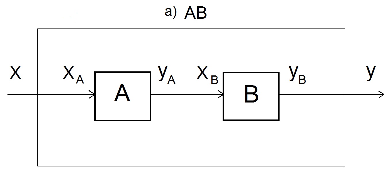
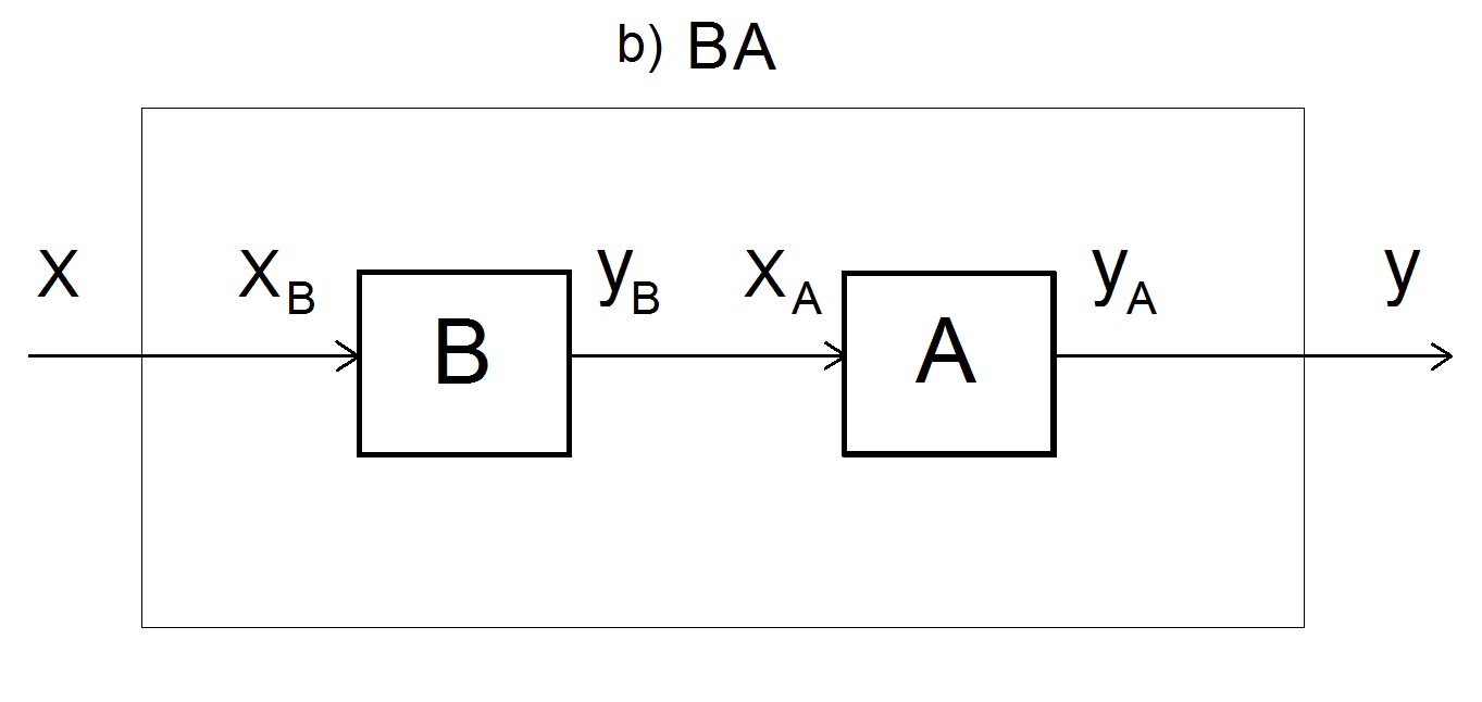
Figure 1. Cascade connection of $A$ and $B;$ $a$) $AB$, $b$) $BA$

Due to the connection in Fig. $1a$, it is obvious that

(2.6) $$x_{A}(t)=x(t),$$

(2.7) $$y_{A}(t)=x_{B}(t),$$

(2.8) $$y_{B}(t)=y(t).$$

Differentiating Eq. (2.3), we obtain

(2.9) $$b_{2}^{\prime}y_{B}^{\prime\prime}+b_{2}y_{B}^{\prime\prime\prime}+b_{1}^{\prime}y_{B}^{\prime}+b_{1}^{\prime}y_{B}^{\prime\prime}+b_{0}^{\prime}y_{B}+b_{0}y_{B}^{\prime}=x_{B}^{\prime}.$$

From Eq. (2.7), $x_{B}^{\prime}=y_{A}^{\prime},$ and then solving Eq. (2.2) for $y_{A}^{\prime},$ finally using Eq. (2.7), we again obtain

$$x_{B}^{\prime}=y_{A}^{\prime}=\frac{x_{A}-a_{0}y_{A}}{a_{1}}=\frac{x_{A}-a_{0}x_{B}}{a_{1}}$$

(2.10) $$=\frac{1}{a_{1}}\left[x_{A}-a_{0}(b_{2}y_{B}^{\prime\prime}+b_{1}y_{B}^{\prime}+b_{0}y_{B})\right],$$

where the last equality is obtained by using the expression Eq. (2.3) for $x_{B}$. Finally, inserting Eq. (2.10) in Eq. (2.9) and replacing $y_{B}\rightarrow y$, $x_{A}\rightarrow x$ due to Eqs. (2.8) and (2.6), respectively, we obtain the following third-order differential system for the connection $AB$

$$a_{1}b_{2}y^{\prime\prime\prime}+(a_{1}b_{2}^{\prime}+a_{1}b_{1}+a_{0}b_{2})y^{\prime\prime}$$

(2.11) $$+(a_{1}b_{1}^{\prime}+a_{1}b_{0}+a_{0}b_{1})y^{\prime}+a_{1}b_{0}^{\prime}+a_{0}b_{0})y=x,$$

(2.12) $$y(t_{0})=y_{B}(t_{0}),$$

(2.13) $$y^{\prime}(t_{0})=y_{B}^{\prime}(t_{0}),$$

(2.14) $$y^{\prime\prime}(t_{0})=y_{B}^{\prime\prime}(t_{0})=\frac{y_{A}(t_{0})-b_{0}(t_{0})y_{B}(t_{0})-b_{1}(t_{0})y_{B}^{\prime}(t_{0})}{b_{2}(t_{0})}.$$

Eqs. (2.12) and (2.13) are obvious due to Eq. (2.8). Eq. (2.14) is obtained as follows: Due to Eq. (2.8), $y(t_{0})=y_{B}^{\prime\prime}(t_{0})$ which is computed from Eq. (2.3) and inserting $x_{B}(t_{0})=y_{A}(t_{0})$ due to Eq. (2.7).

Similarly, due to the connection in Fig. $1b$, it is obvious that

(2.15) $$x_{B}(t)=x(t),$$

(2.16) $$y_{B}(t)=x_{A}(t),$$

(2.17) $$y_{A}(t)=y(t).$$

Differentiating (2.2) two times and ordering the terms, we obtain

(2.18) $$a_{1}y_{A}^{\prime\prime\prime}+(2a_{1}^{\prime}+a_{0})y_{A}^{\prime\prime}+(a_{1}^{\prime\prime}+2a_{0}^{\prime})y_{A}^{\prime}+a_{0}^{\prime\prime}y_{A}=x_{A}^{\prime\prime}.$$

Since $x_{A}^{\prime\prime}(t)=y_{B}^{\prime\prime}(t)$ due to Eq. (2.16), finding $y_{B}^{\prime\prime}$ from Eq. (2.3), and using Eq. (2.16) again, we have

(2.19) $$x_{A}^{\prime\prime}=y_{B}^{\prime\prime}=\frac{x_{B}-b_{1}y_{B}^{\prime}-b_{0}y_{B}}{b_{2}}=\frac{x_{B}-b_{1}x_{A}^{\prime}-b_{0}x_{A}}{b_{2}}.$$

Next inserting in the value of $x_{A}$ from Eq. (2.2) and the value of $x_{A}^{\prime}$ from derivative of Eq. (2.2) into the above equation, we obtain

(2.20) $$x_{A}^{\prime\prime}=\frac{x_{B}-b_{1}(a_{1}^{\prime}y_{A}^{\prime}+a_{1}y_{A}^{\prime\prime}+a_{0}^{\prime}y_{A}^{\prime}+a_{0}y_{A}^{\prime})-b_{0}(a_{1}y_{A}^{\prime}+a_{0}y_{A})}{b_{2}}.$$

Inserting Eq. (2.20) in (2.18) and noting $y_{A}=y$ (Eq. (2.17)) and $x_{B}=x$, (Eq. (2.15)), we obtain the third-order differential equation describing $BA$ as

$$a_{1}b_{2}y^{\prime\prime\prime}+(2a_{1}^{\prime}b_{2}+a_{0}b_{2}+a_{1}b_{1})y^{\prime\prime}$$

(2.21) $$+(a_{1}^{\prime\prime}b_{2}+2a_{0}^{\prime}b_{2}+a_{1}^{\prime}b_{1}+a_{0}b_{1}+a_{1}b_{0})y^{\prime}+(a_{0}^{\prime\prime}b_{2}+a_{0}^{\prime}b_{1}+a_{0}b_{0})y=x,$$

(2.22) $$y(t_{0})=y_{A}(t_{0}),$$

(2.23) $$y^{\prime}(t_{0})=y_{A}^{\prime}(t_{0})=\frac{y_{B}(t_{0})-a_{0}(t_{0})y_{A}(t_{0})}{a_{1}(t_{0})},$$

$$y^{\prime\prime}(t_{0})=y_{A}^{\prime\prime}(t_{0})=\frac{1}{a_{1}(t_{0})}y_{B}^{\prime}(t_{0})-\frac{a_{0}(t_{0})+a_{1}^{\prime}(t_{0})}{a_{1}^{2}(t_{0})}y_{B}(t_{0})$$

(2.24) $$+\left[\frac{a_{0}^{2}(t_{0})+a_{1}^{\prime}(t_{0})a_{0}(t_{0})}{a_{1}^{2}(t_{0})}-\frac{a_{0}^{\prime}(t_{0})}{a_{1}(t_{0})}\right]y_{A}(t_{0}).$$

The derivative of the initial conditions in Eqs. (2.22)-(2.24) is done as follows: Eq. (2.22) follows from Eq. (2.17). To find Eq. (2.22), we start from Eq. (2.17) and write $y^{\prime}(t)=y_{A}^{\prime}(t_{0})$, from Eq. (2.2)

(2.25) $$y(t)=y_{A}^{\prime}(t)=\frac{x_{A}(t)-a_{0}(t)y_{A}(t)}{a_{1}(t)}=\frac{y_{B}(t)-a_{0}(t)y_{A}(t)}{a_{1}(t)}.$$

Inserting $t=t_{0}$ yields Eq. (2.23). To find Eq. (2.24), we start from Eq. (2.17), take derivative of Eq. (2.2) and solve result for $y_{A}^{\prime\prime}$

(2.26) $$y^{\prime\prime}=y_{A}^{\prime\prime}=\frac{y_{B}^{\prime}-(a_{1}^{\prime}+a_{0})y_{A}^{\prime}-a_{0}^{\prime}y_{A}}{a_{1}}.$$

Using the expression Eq. (2.25) for $y_{A}^{\prime}$ in Eq. (2.26), ordering the terms and evaluating at $t=t_{0}$ yields the initial conditions in Eq. (2.24).

3. Commutativity Requirements

For the commutativity of subsystem $A$ and $B$, their combinations $AB$ and $BA$ must have the same outputs for general values of the same input and the same initial conditions. This is due to the existence of unique equal solutions of differential equations derived in Eqs. (2.11)-(2.14) and (2.21)-(2.24) for the same input and initial conditions. Hence, equating the coefficients of these differential equations, collecting the like terms we result with

(3.1) $$a_{1}b_{2}^{\prime}=2a_{1}^{\prime}b_{2}$$

(3.2) $$a_{1}b_{1}^{\prime}=a_{1}^{\prime}b_{1}+(a_{1}^{\prime\prime}+2a_{0}^{\prime})b_{2}$$

(3.3) $$a_{1}b_{0}^{\prime}=a_{0}^{\prime\prime}b_{2}+a_{0}^{\prime}b_{1}$$

(3.4) $$y=y_{B}=y_{A}$$

(3.5) $$y^{\prime}=y_{B}^{\prime}=\frac{y_{B}-a_{0}y_{A}}{a_{1}},$$

(3.6) $$y^{\prime\prime}=\frac{y_{A}-b_{0}y_{B}-b_{1}y_{B}^{\prime}}{b_{2}}=\frac{1}{a_{1}}y_{B}^{\prime}-\frac{a_{0}+a_{1}^{\prime}}{a_{1}^{2}}y_{B}+\left(\frac{a_{0}^{2}+a_{0}a_{1}^{\prime}-a_{0}^{\prime}a_{1}}{a_{1}^{2}}\right)y_{A}$$

Note that Eqs. (3.4)-(3.6) (so should (3.7)-(3.10)) should be valid at the initial time $t=t_{0}$ which is not shown explicitly. Before proceeding further we simplify Eqs. (3.4)-(3.6) to obtain simpler set of constraints.

(3.7) $$y=y_{B}=y_{A},$$

(3.8) $$y^{\prime}=y_{B}^{\prime}=\frac{1-a_{0}}{a_{1}}y_{A},$$

(3.9) $$y^{\prime\prime}=\left[\frac{1-b_{0}}{b_{2}}-\frac{b_{1}(1-a_{0})}{b_{2}a_{1}}\right]y_{A}=\frac{(1-a_{0})(1-a_{0}-a_{1}^{\prime})-a_{0}^{\prime}a_{1}}{a_{1}^{2}}y_{A}.$$

Hence, Eq. (3.9) requires.

(3.10) $$\left[\frac{1-b_{0}}{b_{2}}-\frac{b_{1}(1-a_{0})}{b_{2}a_{1}}-\frac{(1-a_{0})(1-a_{0}-a_{1}^{\prime})-a_{0}^{\prime}a_{1}}{a_{1}^{2}}+\frac{a_{0}^{\prime}}{a_{1}}\right]y_{A}=0.$$

4. Explicit Commutativity Requirements

Eq. (3.1) has a solution for $b_{2}$ in terms of $a_{i}$’s as

(4.1) $$b_{2}=e_{2}a_{1}^{2},$$

where $c_{2}$ is an arbitrary non-zero constant. Using this solution in (3.2) and taking integral, we proceed

$$a_{1}b_{1}^{\prime}=a_{1}^{\prime}b_{1}+(a_{1}^{\prime\prime}+2a_{0}^{\prime})e_{2}a_{1}^{2}$$

$$\frac{a_{1}b_{0}^{\prime}-a_{1}^{\prime}b_{1}}{a_{1}^{2}}=e_{2}(a_{1}^{\prime\prime}+2a_{0}^{\prime})$$

$$\frac{d}{dt}\left(\frac{b_{1}}{a_{1}}\right)=e_{2}(a_{1}^{\prime\prime}+2a_{0}^{\prime})$$

$$\frac{b_{1}}{a_{1}}=e_{2}(a_{1}^{\prime}+2a_{0})+e_{1}$$

(4.2) $$b_{1}=e_{2}(a_{1}^{\prime}+2a_{0})a_{1}+e_{1}a_{1}.$$

Inserting values of $b_{2}$ in Eq. (4.1) and $b_{1}$ in Eq. (4.2) into Eq. (3.3), we proceed

$$a_{1}b_{0}^{\prime}=a_{1}^{\prime\prime}e_{2}a_{1}^{2}+a_{0}^{\prime}\left[e_{2}(a_{1}^{\prime}+2a_{0})a_{1}+e_{1}a_{1}\right]$$

$$b_{0}^{\prime}=a_{1}^{\prime\prime}e_{2}a_{1}+a_{0}^{\prime}\left[e_{2}(a_{1}^{\prime}+2a_{0})+e_{1}\right]$$

$$=e_{2}\left(a_{1}^{\prime\prime}+a_{0}^{\prime}a_{1}^{\prime}+2a_{0}a_{0}^{\prime}\right)+e_{1}a_{0}^{\prime}=e_{2}\frac{d}{dt}(a_{0}^{\prime}a_{1}+a_{0}^{2})+e_{1}a_{0}^{\prime},$$

(4.3) $$b_{0}=e_{2}(a_{0}^{\prime}a_{1}+a_{0}^{2})+e_{1}a_{0}^{\prime}+e_{0},$$

where $e_{0}$ is an integration constant. In the matrix form

(4.4) $$\left[\begin{array}[]{c}b_{2}\\ b_{1}\\ b_{0}\end{array}\right]=\left[\begin{array}[]{ccc}a_{1}^{2}&0&0\\ a_{0}^{\prime}+2a_{0}&1&0\\ a_{0}^{\prime}a_{1}+a_{0}^{2}&a_{0}^{\prime}&1\end{array}\right]\left[\begin{array}[]{c}e_{2}\\ e_{1}\\ e_{0}\end{array}\right].$$

Hence, Eqs. (3.1)-(3.3) are equivalently replaced by Eq. (4.4). Inserting values of $b_{2}$, $b_{1}$, $b_{0}$ computed in Eqs. (4.1)-(4.3) in Eq. (3.10), after simplification, we result with

(4.5) $$\left(e_{2}+e_{1}+e_{0}-1\right)y(t_{0})=0.$$

Since, $t_{0}$ is any initial state for non-zero initial conditions $y_{A}(t_{0})=y_{B}(t_{0})=y(t_{0})\neq 0,$ ($y_{B}^{\prime}(t_{0})$ may be zero if $a_{0}=1$ due to Eq. (3.8), Eq. (4.5) implies that

(4.6) $$e_{2}+e_{1}+e_{0}=1.$$

If commutativity with non-zero initial conditions is to be satisfied. Hence, Eq. (3.10) can be relaced by

(4.7) $$y_{B}(t_{0})=y_{A}(t_{0})\neq 0$$

(4.8) $$y_{B}^{\prime}(t_{0})=\frac{1-a_{0}}{a_{1}}y_{A}(t_{0}),$$

(4.9) $$e_{2}+e_{1}+e_{0}=1,$$

(4.10) $$y^{\prime\prime}=\frac{(1-a_{0})(1-a_{0}-a_{1}^{\prime})-a_{0}^{\prime}a_{1}}{a_{1}^{2}}y_{A}(t_{0}).$$

5. Decomposition Formulas

We now express the coefficients of the decompositions $A$ and $B$ in terms of these of the decomposed system $C$. Comparing Eqs. (2.1) and (2.11), equating the coefficients of third derivatives, and using Eq. (4.4), we have

(5.1) $$a_{1}b_{2}=c_{3}=a_{1}e_{1}a_{1}^{2}\rightarrow a_{1}=\left(\frac{c_{3}}{e_{2}}\right)^{1/3}.$$

Comparing Eqs. (2.1) and (2.11), equating the coefficients of second derivatives, and using Eq. (4.4), we obtain

$$a_{1}b_{2}^{\prime}+a_{1}b_{1}+a_{0}b_{2}=c_{2}\rightarrow a_{0}=\frac{1}{b_{2}}\left(c_{2}-a_{1}b_{2}^{\prime}-a_{1}b_{1}\right)$$

$$=\frac{1}{e_{2}a_{1}^{2}}\left\{c_{2}-a_{1}\frac{d}{dt}\left(e_{2}a_{1}^{2}\right)-a_{1}e_{2}[(a_{1}^{\prime}+2a_{0})a_{1}+e_{1}a_{1}]\right\}$$

$$=\frac{1}{e_{2}a_{1}^{2}}\left[c_{2}-2e_{2}a_{1}^{2}a_{1}^{\prime}-e_{2}a_{1}^{2}(a_{1}^{\prime}+2a_{0})-a_{1}^{2}\right]$$

$$=\frac{1}{e_{2}}\left(\frac{c_{2}}{a_{1}^{2}}-2e_{2}a_{1}^{\prime}-e_{2}a_{1}^{\prime}-2e_{2}a_{0}-e_{1}\right)=\frac{c_{2}}{e_{2}a_{1}^{2}}-3a_{1}^{\prime}-2a_{0}-\frac{e_{1}}{e_{2}}$$

$$3a_{0}=\frac{c_{2}}{e_{2}a_{1}^{2}}-3a_{1}^{\prime}-\frac{e_{1}}{e_{2}}.$$

Dividing by $3$ and using Eq. (5.1), we proceed as

$$a_{0}=\frac{c_{2}}{e_{2}a_{1}^{2}}-a_{1}^{\prime}-\frac{e_{1}}{3e_{2}}=\frac{(e_{2})^{1/3}c_{2}}{3e_{2}(c_{3})^{2/3}}-\frac{1}{3}\left(\frac{c_{3}}{e_{2}}\right)^{-2/3}\frac{c_{3}^{\prime}}{e_{2}}-\frac{e_{1}}{3e_{2}}$$

(5.2) $$=\frac{c_{2}}{3e_{2}^{1/3}c_{3}^{2/3}}-\frac{c_{3}^{\prime}}{3c_{3}^{2/3}e_{2}^{1/3}}-\frac{e_{1}}{3e_{2}}=\frac{c_{2}-c_{3}^{\prime}}{3e_{2}^{1/3}c_{3}^{2/3}}-\frac{e_{1}}{3e_{2}}.$$

Having computing $a_{1}$ and $a_{0}$ in Eqs. (5.1) and (5.2), inserting those values in Eq. (4.4), we compute $b_{2}$, $b_{1}$, $b_{0}$ and the results:

(5.3) $$b_{2}=3e_{2}^{1/3}c_{3}^{2/3},$$

(5.4) $$b_{1}=\frac{1}{3}\left[\left(\frac{e_{2}}{c_{3}}\right)^{1/3}\left(2c_{2}-c_{3}^{\prime}\right)+e_{1}\left(\frac{c_{3}}{e_{2}}\right)^{1/3}\right],$$

$$b_{0}=\frac{1}{9}\left[\left(\frac{e_{2}}{c_{3}}\right)^{1/3}\left(3c_{2}^{\prime}-3c_{3}^{\prime\prime}\right)+\frac{c_{2}^{2}+\left(c_{3}^{\prime}\right)^{2}-4c_{2}c_{3}^{\prime}}{c_{3}}\right]$$

(5.5) $$+\frac{1}{9}\left[\frac{e_{1}(c_{2}-c_{3}^{\prime})}{e_{2}^{1/3}c_{3}^{2/3}}-\frac{2e_{1}^{2}}{e_{2}}\right]+e_{0}.$$

Comparing Eq. (2.1) with Eq. (2.11), two additional equations should be satisfied for the equivalence of $C$ and $AB$ (or $BA$, since $AB$ is a commutative pair). These are

(5.6) $$c_{1}=a_{1}b_{1}^{\prime}+a_{1}b_{0}+a_{0}b_{1},$$

(5.7) $$c_{0}=a_{1}b_{0}^{\prime}+a_{0}b_{0}.$$

Inserting the valves of $a_{1}$, $a_{0}$ in Eqs. (5.1), (5.2) and $b_{1}$, $b_{0}$ as computed in Eqs. (5.4), (5.5) into Eqs. (5.6) and (5.7) and making a grate deal of computations, we obtain the additional conditions to be satisfied;

(5.8) $$c_{1}=\left(c_{2}^{\prime}-\frac{2}{3}c_{3}^{\prime\prime}\right)+\frac{1}{c_{3}}\left[\frac{5}{9}\left(c_{3}^{\prime}\right)^{2}-c_{2}c_{3}^{\prime}+\frac{c_{2}^{2}}{3}\right]+c_{3}^{1/3}\frac{1}{e_{2}^{1/3}}\left(e_{0}-\frac{e_{1}^{2}}{3e_{2}}\right),$$

$$c_{0}=\frac{1}{3}\left(c_{2}^{\prime\prime}-c_{3}^{\prime\prime\prime}\right)+\frac{1}{3c_{3}}(c_{2}-2c_{3}^{\prime})(c_{2}^{\prime}-c_{3}^{\prime\prime})$$

$$+\frac{1}{27c_{3}^{2}}\left[15\left(c_{3}^{\prime}\right)^{2}-8c_{3}^{\prime}c_{2}-6c_{3}^{\prime\prime}c_{2}+c_{2}^{2}\right](c_{2}-c_{2}^{\prime})$$

(5.9) $$+\frac{c_{2}-c_{3}^{\prime}}{3c_{3}^{2/3}b_{2}e_{2}^{1/3}}\left(e_{0}-\frac{e_{1}^{2}}{3e_{2}}\right)+\frac{e_{1}}{3}\left(\frac{2e_{1}^{2}}{9}-\frac{e_{0}}{e_{2}}\right).$$

In the light of the result obtained so far, we now express the main theorem about the decomposition of a third-order linear time-varying system into its commutative first and second-order linear time-varying components.

Theorem 1.

The necessary and sufficient conditions that a third-order linear time-varying system described by Eq. (2.1) into its cascade connected linear time-varying commutative pairs of first-order and second-order are that

i):

The coefficient $c_{1}$ and $c_{0}$ be expressible in terms of $c_{3}$ and $c_{2}$ through formulas Eqs. (5.8) and (5.9) where $e_{2}$, $e_{1}$, $e_{0}$ are some constants.

ii):

If the condition $y(t_{0})$ of $C$ is different from zero, additional necessary and sufficient condition are expressed as

(5.10) $$e_{2}+e_{1}+e_{0}=1,$$

(5.11) $$y^{\prime}(t_{0})=\left[\left(\frac{e_{2}}{c_{3}}\right)^{1/3}\left(1+\frac{e_{1}}{3e_{2}}\right)-\frac{c_{2}-c_{3}^{\prime}}{3c_{3}}\right]y(t_{0})\text{ at }t=t_{0},$$

$$y^{\prime}(t_{0})=\left[\left(\frac{e_{2}}{c_{3}}\right)^{1/3}\left(1+\frac{e_{1}}{3e_{2}}\right)-\frac{c_{2}-c_{3}^{\prime}}{3c_{3}}\right]^{2}y_{A}(t_{0})$$

(5.12) $$+\frac{d}{dt}\left[\left(\frac{e_{2}}{c_{3}}\right)^{1/3}\left(1+\frac{e_{1}}{3e_{2}}\right)-\frac{c_{2}-c_{3}^{\prime}}{3c_{3}}\right]y_{A}(t_{0}).$$

Proof.

Part i) is simply re-expressing of Eqs. (5.8) and (5.9). Eq. (5.10) is the repetition of Eq. (4.9). Eq. (5.11) is obtained from Eq. (4.8) by inserting in the valves of $a_{1}$ and $a_{0}$ in Eqs. (5.1) and (5.2), respectively. So,    

$$y^{\prime}(t_{0})=\frac{1-a_{0}}{a_{1}}y(t_{0})=\left(\frac{e_{2}}{c_{3}}\right)^{1/3}\left(1+\frac{e_{1}}{3e_{2}}-\frac{c_{2}-c{{}^{\prime}}_{3}}{3e_{2}^{1/3}c_{3}^{2/3}}\right)y(t_{0})$$

$$=\left[\left(\frac{e_{2}}{c_{3}}\right)^{1/3}\left(1+\frac{e_{1}}{3e_{2}}\right)-\frac{c_{2}-c_{3}^{\prime}}{3c_{3}}\right]y(t_{0}).$$

Finally, Eq. (5.12) is obtained from From Eq. (4.9) by inserting in valves of $a_{1}$ and $a_{0}$ in Eqs. (5.1) and (5.2), respectively as follows:

$$y^{\prime\prime}(t_{0})=\frac{\left(1-a_{0}\right)\left(1-a_{0}-a_{1}^{\prime}\right)-a_{0}^{\prime}a_{1}}{a_{1}^{2}}y_{A}(t_{0})$$

$$=\frac{(1-a_{0})^{2}-a_{1}^{\prime}+a_{0}a_{1}^{\prime}-a_{0}^{\prime}a_{1}}{a_{1}^{2}}y_{A}(t_{0})$$

$$=\left[\frac{(1-a_{0})^{2}}{a_{1}^{2}}+\frac{d}{dt}\frac{1}{a_{1}}-\frac{d}{dt}\frac{a_{0}}{a_{1}}\right]y_{A}(t_{0})=\left[\frac{(1-a_{0})^{2}}{a_{1}^{2}}+\frac{d}{dt}\frac{1-a_{0}}{a_{1}}\right]y_{A}(t_{0})$$

$$=\left[\left(\frac{e_{2}}{c_{3}}\right)^{1/3}\left(1+\frac{e_{1}}{3e_{2}}\right)-\frac{c_{2}-c_{3}^{\prime}}{3c_{3}}\right]^{2}y_{A}(t_{0})$$

$$+\frac{d}{dt}\left[\left(\frac{e_{2}}{c_{3}}\right)^{1/3}\left(1+\frac{e_{1}}{3e_{2}}\right)-\frac{c_{2}-c_{3}^{\prime}}{3c_{3}}\right]y_{A}(t_{0}).$$

The second theorem expresses how to obtain the commutative pairs of decomposition $A$ and $B$.

Theorem 2.

For a third-order linear time-varying system $C$ described by Eq.(2.1) with the conditions of Theorem I satisfied, the decomposed commutative pairs $A$ and $B$ are found by Eqs. (5.1) and (5.2) for the coefficients $a_{1}$ and $a_{0}$ of $A$, and by Eqs. (5.3), (5.4), (5.5) for the coefficients of $b_{2}$ , $b_{1}$, $b_{0}$ of $B$, all respectively. Further, for the commutative decompositions with non-zero initial condition $y(t_{0})\neq 0$, Eq. (5.10) relating the constants $e_{2}$, $e_{1}$, $e_{0}$ must be satisfied; and $y_{B}^{\prime}(t_{0})=y^{\prime}(t_{0})$ and $y^{\prime\prime}(t_{0})$ must be expressible in terms of $y(t_{0})=y_{B}(t_{0})=y_{A}(t_{0})$ as in Eqs. (5.11) and (5.12), respectively.

Proof.

The proof follows from the development of the mentioned equation. Equality of $y(t_{0})=y_{B}(t_{0})=y_{A}(t_{0})$ is a result of Eqs. (2.12) and (2.15); equality of $y^{\prime}(t_{0})=y_{A}^{\prime}(t_{0})$ is already expressed in Eq. (2.12).    

6.
Examples

In this section, four examples are considered to illustrate the results of the paper. The simulations are conducted by MATLAB R2012a and obtained by a PC Intel${}^{\ooalign{\hfil\raise 0.21098pt\hbox{$\scriptstyle\mathrm{\text{missing}}{R}$}\hfil\crcr\text{$\mathchar 525\relax$}}}$ Core™ i3 CPV, 2.13 GHz, 3.86 GB of RAM well verify the results.

6.1.
Example 1

Let $C$ be the third-order linear time-varying system defined by

(6.1) $$y^{\prime\prime\prime}(t)+(t+1)y^{\prime\prime}(t)+\frac{1}{3}(t^{2}+2t)y^{\prime}(t)+\frac{1}{27}\left(t^{3}+3t^{2}+9\right)y(t)=x(t),$$

which the coefficients are

(6.2) $$c_{3}=1,\text{ }c_{2}=(t+1),\text{ }c_{1}=\frac{1}{3}(t^{2}+2t),\text{ }c_{0}=\frac{1}{27}(t^{3}+3t^{2}+9),$$

with the constants

(6.3) $$e_{2}=e_{1}=1,\text{ }e_{0}=-1,$$

which satisfies Eq. (5.10), it is true the conditions $i)$ of Theorem I are satisfied; that is $c_{1}$ and $c_{0}$ satisfy Eqs. (5.8) and (5.9), respectively. For the validity of the decomposition with non-zero initial condition $y(t_{0})\neq 0,$ condition (5.10) of $ii)$ is satisfied by the constant chosen in Eq. (6.3). Further, Eqs. (5.11) and (5.12) of $ii)$ together with Theorem 2 yield

(6.4) $$y_{A}(t_{0})=y_{B}(t_{0})=y(t_{0}),$$

$$y_{B}^{\prime}(t_{0})=y^{\prime}(t_{0})=\left[\left(\frac{1}{1}\right)^{1/3}\left(1+\frac{1}{3}\right)-\frac{t_{0}+1}{3}\right]y(t_{0})$$

(6.5) $$=\left(1-\frac{t_{0}}{3}\right)y(t_{0})=y(t_{0})\text{ for }t_{0}=0,$$

$$y^{\prime\prime}(t_{0})=\left[\left(1+\frac{1}{3}-\frac{t_{0}+1}{3}\right)^{2}+\frac{d}{dt}\left.\left(1+\frac{1}{3}-\frac{t+1}{3}\right)\right|_{t=t_{0}}\right]y(t_{0})$$

$$=\left[\left(1-\frac{t_{0}}{3}\right)^{2}+\frac{d}{dt}\left.\left(1-\frac{t}{3}\right)\right|_{t=t_{0}}\right]y(t_{0})$$

(6.6) $$=\left[\left(1-\frac{t_{0}}{3}\right)^{2}-\frac{1}{3}\right]y(t_{0})=\frac{2}{3}y(t_{0})\text{ for }t_{0}=0.$$

Theorem 2 yields the following coefficients for decomposed subsystem $A$ and $B:$

(6.7) $$A:y_{A}^{\prime}(t)+\frac{t}{3}y_{A}(t)=x_{A}(t),$$

(6.8) $$B:y_{B}^{\prime\prime}(t)+\frac{2t+3}{3}y_{B}^{\prime}(t)+\frac{t^{2}+3t-6}{9}y_{B}(t)=x_{B}(t).$$

Simulations are carried out with a sinusoidal input of amplitude $10$, bias $-5$ and frequency $3$. Fixed step length of $0.01$ is used by ode(Bogacki-Shampine). Simulink results of MATLAB R2012 are shown in Fig. 2. The initial time $t_{0}$ is assumed $1$ and the initial states are taken as $y(1)=y_{A}(1)=y_{B}(1)=1$. When $y_{B}^{\prime}(1)=y^{\prime}(1)=1$ and $y^{\prime\prime}(1)=2/3$ as implied by (6.4), (6.5), (6.6) all the decomposition conditions are satisfied and $AB,$ $BA,$ and $C$ give the same responses as indicated by the figure legend. But when $y^{\prime\prime}(1)$ is changed to $2$ which does not satisfy (6.6), the response $C1$ becomes different from those of $AB$ and $BC$, that is the decomposition get spoiled; although $A$ and $B$ are commutative, they are not the correct decomposition of $C$. On the other hand, when $y_{B}^{\prime}(1)$ is made $-1$, that is (6.5) is not satisfied, the response of $AB$ (indicated by $AB3$) gets different from those of $BA$ and $C$, so commutative decomposition of $C$ into $A$ and $B$ is not valid again.

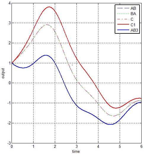
Figure 2. Decomposition of $C$ into its commutative pairs $A$ and $B$ ($AB,BA,C$); some of the conditions of decomposition are not satisfied ($C1,$ $AB3$)

6.2. Example 2

Consider $C$ defined by

(6.9) $$t^{3}y^{\prime\prime\prime}(t)+7t^{2}y^{\prime\prime}(t)+9ty^{\prime}(t)+y(t)=x(t),$$

which satisfies the condition of Theorem I with $e_{2}=e_{1}=1,$ $e_{0}=-1.$ Hence, with $c_{3}=t^{3},$ $c_{2}=7t^{2},$ the initial conditions should satisfy Eqs. (5.11) and (5.12):

(6.10) $$y^{\prime}(t_{0})=\left[\frac{1}{t_{0}}\left(1+\frac{1}{3}\right)-\frac{7t_{0}^{2}-3t_{0}^{2}}{3t_{0}^{3}}\right]y(t_{0})=0,$$

$$y^{\prime\prime}(t_{0})=\left\{\left[\frac{1}{t_{0}}\left(1+\frac{1}{3}\right)-\frac{7t_{0}^{2}-3t_{0}^{2}}{3t_{0}^{3}}\right]^{2}\right.$$

(6.11) $$\left.+\frac{d}{dt}\left.\left[\frac{1}{t}\left(1+\frac{1}{3}\right)-\frac{7t^{2}-3t^{2}}{3t^{3}}\right]\right|_{t=t_{0}}\right\}y(t_{0})=0.$$

The decompositions $A$ and $B$ are found by using Eqs. (5.1), (5.2) and (5.3)-(5.5) as

(6.12) $$A:ty_{A}^{\prime}(t)+y_{A}(t)=x_{A}(t),\text{ }y_{A}(t_{0})=y\left(t_{0}\right),$$

(6.13) $$B:t^{2}y_{B}^{\prime\prime}(t)+4ty_{B}^{\prime}(t)+y_{B}(t)=x_{B}(t),y_{B}(t_{0})=y\left(t_{0}\right),\text{ }y_{B}^{\prime}(t_{0})=y^{\prime}\left(t_{0}\right)=0.$$

Note that $y^{\prime}(t_{0})=y_{B}^{\prime}\left(t_{0}\right),$ $y^{\prime\prime}(t_{0})$ are zero for all initial times $t_{0}.$ The simulations are carried out with a sinusoidal input of amplitude $100$, frequency $100$ Hz and phase $\pi/3$ rad; the initial time $t_{0}$ is taken as $0.01$ and stop time is $0.15$; ode(Bogacki-Shampine) solver is used with step-length of $0.001.$ The initial values are assumed as $y_{A}(t_{0})=y_{B}(t_{0})=y(t_{0})=-4$. As it is seen in Fig. 3, $C$ and its commutative decompositions $AB$ and $BA$ yield the same responses (see $AB=BA=C$). When the decomposition requirement on initial condition get spoiled, that is $y^{\prime}(0.01)=y_{B}^{\prime}(0.01)\neq 0$ and taken as $-100$, the decomposition is not valid at all as seen from plots $AB1,$ $BA1,$ $C1$ in the figure. It is important to note that the cascade connection $BA$ is least affected from this change. Hence, it is preferable decomposition or synthesis of $C$ when compared with $AB$ as far as sensitivity to initial conditions is concerned.

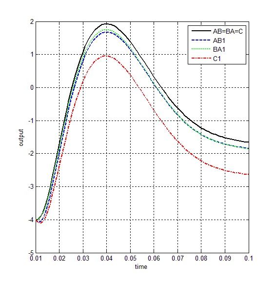
Figure 3. Simulation result for Example 2 when decomposition requirements are satisfied ($AB=BA=C$) and they are not satisfied ($AB1,BA1,C1$)

6.3. Example 3

Let $C$ be the third-order Euler system defined by

(6.14) $$t^{3}y^{\prime\prime\prime}+9t^{2}y^{\prime\prime}+\frac{53}{3}ty^{\prime}+\frac{155}{27}y=x.$$

Comparing it with (2.1), its coefficients are

(6.15) $$c_{3}=t^{3},\text{ }c_{2}=9t^{2},\text{ }c_{1}=\frac{53}{3}t,\text{ }c_{0}=\frac{155}{27}.$$

It is true that the choice $e_{2}=e_{1}=1,$ $e_{0}=-1$ satisfy the conditions of Theorem I; that is Eqs. (5.8), (5.9) and (5.10) are satisfied. Hence, the decomposition into first and second-order commutative pairs with non-zero initial condition $y(t_{0})\neq 0$ is possible. The initial condition of $A$ and $B$ as well as those of $C$ are found by using Theorem I and II. In fact,

(6.16) $$y_{A}(t_{0})=y_{B}(t_{0})=y(t_{0})\neq 0,$$

(6.17) $$y_{B}^{\prime}(t_{0})=y^{\prime}(t_{0})=\left[\left(\frac{1}{t_{0}^{3}}\right)^{1/3}\left(1+\frac{1}{3}\right)-\frac{9t_{0}^{2}-3t_{0}^{2}}{3t_{0}^{2}}\right]y(t_{0})=-\frac{2}{3t_{0}}y(t_{0}),$$

$$y^{\prime\prime}(t_{0})=\left\{\left[\frac{1}{t_{0}}\left(1+\frac{1}{3}\right)-\frac{3t_{0}^{2}-3t_{0}^{2}-1}{3t_{0}^{2}}\right]^{2}\right.$$

$$\left.+\frac{d}{dt}\left.\left(\frac{1}{t}\frac{4}{3}-\frac{3t^{2}-3t^{2}}{3t^{2}}\right)\right|_{t=t_{0}}\right\}y(t_{0})$$

(6.18) $$=\left(\frac{4}{9t_{0}^{2}}+\frac{2}{3t_{0}^{2}}\right)y(t_{0})=\frac{10}{9t_{0}^{2}}y(t_{0}).$$

The decompositions $A$ and $B$ are found by using the coefficients given in Eqs. (5.1), (5.2) and (5.3)-(5.5). With the above initial conditions $A$ and $B$ are defined by

(6.19) $$A:ty_{A}^{\prime}(t)+\frac{5}{3}y_{A}(t)=x_{A}(t);\text{ }y_{A}(t_{0})=y(t_{0}),$$

$$B:t^{2}y_{B}^{\prime\prime}(t)+\frac{16}{3}ty_{B}^{\prime}(t)+\frac{31}{9}y_{B}(t)=x_{B}(t);$$

(6.20) $$\text{ }y_{B}(t_{0})=y(t_{0});\text{ }y_{B}^{\prime}(t_{0})=y^{\prime}(t_{0})=-\frac{2}{3t_{0}^{2}}y(t_{0}).$$

The simulations are done for sinusoidal input of amplitude $10$ and frequency $1$. The initial time $t_{0}=1;$ ode3(Bogacki-Shampine) solver is used with a fixed step-length of $0.01$; simulations are stopped at $t=10$. When the initial conditions $y^{\prime\prime}(1)=10/9,$ $y^{\prime}(1)=y_{B}^{\prime}(1)=-2/3$ are chosen in accordance with $y_{A}(1)=y_{B}(1)=y(1)=1$ as to satisfy the decomposition above mentioned conditions, $AB,$ $BA,$ $C$ give the same response as shown in Fig. 4 (see $AB=BA=C$). In the same figure, zero input responses ($AB1=BA1=C1$) and zero state responses ($AB2=BA2=C2$) are also potted. Obviously, decomposition is valid for unexited-unrelaxed and exited-relaxed cases as well.

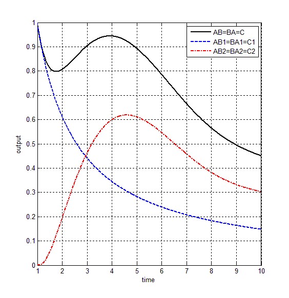
Figure 4. Complete zero-input ($C1$), and zero-state ($C2$) responses of Example 3

6.4. Example 4

This example is the same as the first one except all the initial conditions are taken as zero and a noise signal is added between the junction of subsystems $A$ and $B$. The noise is a pulse sequence with amplitude $4$, $\%$ $50$ pulse with, and a bias of $-2.3$. The simulation results are shown in Fig. 5. Obviously, the interconnection $AB$ is less effected by this noise than $BA$ connection when compared with the output of the original system $C$. Hence, the cascade synthesis $AB$ should be preferred rather than $BA$.

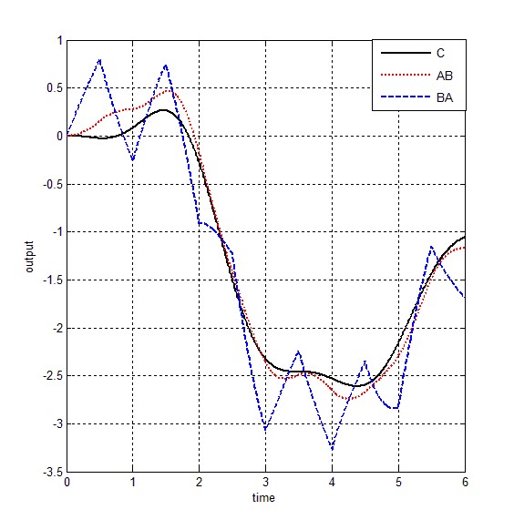
Figure 5. Outputs of the original system $C$ and its cascade decompositions $AB$ and $BA$ when disturbance exists at the interconnection

7.
Conclusions

In this paper, the decomposition of any third-order linear time-varying system into its first and second-order commutative pairs is investigated. Explicit decomposition formulas are derived for the case of zero and non-zero initial conditions. The results are validated by computer simulations. The work is original and appears for the first time in the literature. It is important from the synthesis and/or design point of views of engineering systems. Many design methods are based on tearing and reconstruction, which is combining simple components to obtain an assembly. Further, it is shown that some combinations may be better than the others when sensitivity to initial conditions and noise disturbance at the interconnection is taken into account. On the other hand, commutativity of cascade connected systems have gained a grade deal of interest and its possible benefits have been pointed out on the literature. Hence, the results of this paper can be used readily for beneficial synthesis of third-order linear time-varying systems.

References

[1] Suzuki, A.: Cascade connection of solar collectors for effective
energy gain. Journal of Solar Energy Engineering-Transactions of the ASME.
108, 172-177 (1986).
[2] Gohberg, I., Kaashoek, M.A., Ran, A.C.M.: Partial role and zero
displacement by cascade connection. SIAM Journal on Matrix Analysis and
Applications. 10, 316-325 (1989).
[3] Ninomiya, K., Harada, K., Miyazaki, I.: Stability analysis of an
active filter using cascade connection of switching regulators. Electronics
and Communications in Japan Part I-Communications. 80, 87-94 (1997).
[4] Shi, W.J., Yao, Y., Zhang, T.Q., Meng, X.J.: A method of
recognizing biology surface spectrum using cascade-connection artificial
neural nets. Spectroscopy and Spectral Analysis. 28, 983-987 (2008).
[5] Zhang, J.M., Qi, W.F., Tian, T., Wang, X.Z.: Further Results on
the Decomposition of an NFSR Into the Cascade Connection of an NFSR Into an
LFSR. IEEE Transactions on Information Theory. 61, 645-654 (2015).
[6] Vasileska, D., Goodnick, S.M.: Computational Electronics. Morgan
&Claypool Publishers (2006).
[8] Marshal, E.: Commutativity of time varying systems. Electronics
Letters. 13, 539-540 (1997).
[9] Koksal, M.: Commutativity of second-order time-varying systems.
International Journal of Control. 36, 541-544 (1982).
[10] Salehi, S.V.: Comments on ‘Commutativity of second-order
time-varying systems’. International Journal of Control. 37, 1195-1196
(1983).
[11] Koksal, M.: Corrections on ‘Commutativity of second-order
time-varying systems’. International Journal of Control. 38, 273-274 (1983).
[12] Koksal, M.: General conditions for commutativity of
time-varying systems. Proceedings of the International Conference on
Telecommunication and Control, Halkidiki, Greece, 223-225 (1984)
[13] Koksal, M.: A Survey on the commutativity of time-varying
systems. METU, Gaziantep Engineering Faculty, Technical. Report no: GEEE
CAS-85/1, (1985).
[14] M. Koksal, An exhaustive study on the commutativity of
time-varying systems, International Journal of Control, 47 (1988) 1521-1537.
[15] Koksal, M., Koksal, M.E.: Commutativity of linear time-varying
differential systems with non-zero initial conditions: A review and some new
extensions. Mathematical Problems in Engineering. 2011, 1-25 (2011).
[16] Koksal, M.E.: Decomposition of a second-order linear
time-varying differential system as the series connection of two first-order
commutative pairs. Open Mathematics. 14, 693-704 (2016).
[17] Koksal, M., Koksal, M.E.: Commutativity of cascade connected
discrete time linear time-varying systems (in Turkish). 2013 Automatic
Control National Meeting TOK”2013, Malatya-Turkey, 1128-1131 (2013).
[18] Koksal, M., Koksal, M.E.: Commutativity of cascade connected
discrete time linear time-varying systems. Transactions of the Institute of
Measurement and Control. 37, 615-622 (2015).