Robust approximation error estimates and multigrid solvers for isogeometric multi-patch discretizations

Abstract

In recent publications, the author and his coworkers have shown robust approximation error estimates for B-splines of maximum smoothness and have proposed multigrid methods based on them. These methods allow to solve the linear system arizing from the discretization of a partial differential equation in Isogeometric Analysis in a single-patch setting with convergence rates that are provably robust both in the grid size and the spline degree. In real-world problems, the computational domain cannot be nicely represented by just one patch. In computer aided design, such domains are typically represented as a union of multiple patches. In the present paper, we extend the approximation error estimates and the multigrid solver to this multi-patch case.

1 Introduction

The key idea of Isogeometric Analysis (IgA), [19], is to unite the world of computer aided design (CAD) and the world of finite element (FEM) simulation. Spline spaces, such as spaces spanned by tensor product B-splines or NURBS, are typically used for geometry representation in standard CAD systems. In classical IgA, both the computational domain and the solution of the partial differential equation (PDE) are represented by spline functions.

More complicated domains cannot be represented by just one such (tensor-product) spline function. Instead, the whole domain is decomposed into subdomains, in IgA typically called patches, where each of them is represented by its own geometry function. This is called the multi-patch case, in contrast to the single-patch case.

Concerning the approximation error, in early IgA literature, only its dependence on the grid size has been studied, cf. [19, 1]. In recent publications [2, 25, 11] also the dependence on the spline degree has been investigated. These error estimates are restricted to the single-patch case. We will extend the results from [25] on approximation errors for B-splines of maximum smoothness to the multi-patch case.

As a next step, the linear system resulting from the isogeometric discretization of the PDE has to be solved. Several solvers have been proposed for the multi-patch case, typically established solution strategies known from the finite element literature, including direct solvers [3] or non-overlapping and overlapping domain decomposition methods [4, 5, 6], FETI-like approaches (called IETI in the IgA context) [20]. The solution of local subproblems in such domain decomposition methods is done with general direct solvers, fast direct solvers exploiting the tensor product structure, cf. [22], or again iterative solvers, like multigrid or multilevel methods, cf. [14] for multigrid methods in the framework of a IETI solver.

To apply multigrid methods directly to the system arizing from a multi-patch discretization, is an appealing alternative. If standard smoothers known from finite elements (Jacobi, Gauss Seidel) are used, the extension of the multigrid methods to multi-patch IgA discretizations is straight-forward. However, it is well known that their convergence rates deteriorate dramatically if $p$ is increased, cf. [12, 18, 17].

A robust and efficient multigrid solver for the single-patch case was presented in [16]; alternatives include [10, 17]. Based on a robust inverse inequality and a robust approximation error estimate in a large subspace of the whole spline space (from [25]), it was shown that mass matrices can be used as robust smoothers in this large subspace. For the other subspaces, particular smoothers have been proposed, which can capture the outlier frequencies on the one hand and which still have tensor product structure on the other hand. The overall smoother is then obtained by combining them by an additive Schwarz type approach.

That multigrid smoother relies on the tensor-product structure of the mass matrix and is, therefore, restricted to the single-patch case. We will set up instances of that smoother for each patch and will combine them in an additive Schwarz type way to obtain a multi-patch multigrid smoother. This smoother will be used in a standard multigrid framework living on the whole multi-patch domain. We will discuss the convergence rates of the multigrid solver and its overall computational complexity.

Multigrid methods are typically known as optimal methods, which means that their overall computational complexity grows linearly with the number of unknowns. If also the dependence in the spline degree is of interest, the best we can expect is that the multigrid method is not more expensive than the computation of the residual, which requires the multiplication with the stiffness matrix. In two dimensions, the stiffness matrix has $\mathcal{O}(Np^{2})$ non-zero entries, where $N$ is the number of unknowns, $p$ is the spline degree, and $\mathcal{O}(\cdot)$ is the Landau notation. So, we call the multigrid method optimal if we can show that its overall complexity is not more than $\mathcal{O}(Np^{d})$.

The remainder of the paper is organized as follows. First, the model problem and the discretization are discussed in Section 2. Then, in Section 3, a robust approximation error estimate for the multi-patch domain is given. These results are used in Section 4 to set up a multigrid method for the multi-patch domain. In Section 5, we give numerical experiments for the multigrid method and in Section 6, we draw conclusions.

2 Preliminaries

In this paper, we consider the following Poisson model problem. For a given function $f$, we are interested in the function $u$ solving

$$-\Delta u=f\quad\mbox{ in }\Omega,\qquad u=0\quad\mbox{ on }\partial\Omega,$$

where $\Omega\subset\mathbb{R}^{2}$ is an open, bounded and simply connected Lipschitz domain with boundary $\partial\Omega$. The standard weak form of the model problem reads as follows. Given $f\in L_{2}(\Omega)$, find $u\in H^{1}_{0}(\Omega)$ such that

$$(\nabla u,\nabla v)_{L_{2}(\Omega)}=(f,v)_{L_{2}(\Omega)}\qquad\mbox{for all $v\in H^{1}_{0}(\Omega)$.}$$ (2.1)

Here and in what follows, $L_{2}(\Omega)$, $H^{1}(\Omega)$, $H^{2}(\Omega)$ and $H^{1}_{0}(\Omega)$ are the standard Lebesgue and Sobolev spaces with standard scalar products $(\cdot,\cdot)_{L_{2}(\Omega)}$, $(\cdot,\cdot)_{H^{1}(\Omega)}:=(\nabla\cdot,\nabla\cdot)_{L_{2}(\Omega)}$, norms $\|\cdot\|_{L_{2}(\Omega)}$, $\|\cdot\|_{H^{1}(\Omega)}$, $\|\cdot\|_{H^{2}(\Omega)}$, and seminorm $|\cdot|_{H^{1}(\Omega)}$.

This problem is solved with a standard fully matching multi-patch isogeometric discretization. For sake of completeness and to introduce a notation, we give the details. For simplicity, we restrict ourselves to the two-dimensional case.

Assume that the domain $\Omega\subset\mathbb{R}^{2}$ consists of $K$ patches, denoted by $\Omega_{k}$ for $k=1,\ldots,K$ such that the domain $\Omega$ is covered by non-overlapping patches, i.e.,

$$\overline{\Omega}=\bigcup_{k=1}^{K}\overline{\Omega_{k}}\quad\mbox{and}\quad\Omega_{k}\cap\Omega_{l}=\emptyset\mbox{ for any }k\not=l,$$ (2.2)

where for any domain $T\subset\mathbb{R}^{2}$, the symbol $\overline{T}$ denotes its closure. Each of those patches is represented by a bijective geometry function

$$G_{k}:\widehat{\Omega}:=(0,1)^{2}\rightarrow\Omega_{k}:=G_{k}(\widehat{\Omega})\subset\mathbb{R}^{2},$$

which can be continuously extended to the closure of $\widehat{\Omega}$.

Analogously to [16], we assume that the geometry function is sufficiently smooth such that the following assumption holds.

Assumption 2.1

There is a constant $C_{G}>0$ such that geometry functions $G_{k}$ satisfy

$$C_{G}^{-1}\|v\|_{L_{2}(\widehat{\Omega})}\leq\|v\circ G_{k}^{-1}\|_{L_{2}(\Omega_{k})}\leq C_{G}\|v\|_{L_{2}(\widehat{\Omega})} \;\;\mbox{ for all }v\in L_{2}(\widehat{\Omega})$$

$$C_{G}^{-1}\|v\|_{H^{r}(\widehat{\Omega})}\leq\|v\circ G_{k}^{-1}\|_{H^{r}(\Omega_{k})}\leq C_{G}\|v\|_{H^{r}(\widehat{\Omega})} \;\;\mbox{ for all }v\in H^{r}(\widehat{\Omega}),\,r\in\{1,2\}.$$

As the dependence on the geometry function is not in the focus of this paper, unspecified constants might depend on $C_{G}$.

For any patch $\Omega_{k}$, we denote by $\mathbb{K}_{k}:=\{G_{k}((0,1)^{2})\}=\{\Omega_{k}\}$ its interior, by

$$\mathbb{E}_{k} :=\left\{G_{k}(\Gamma)\;:\;\begin{array}[]{c}\Gamma\in\{\{0\}\times(0,1),\{1\}\times(0,1),(0,1)\times\{0\},(0,1)\times\{1\}\}\\ \mbox{ such that }G_{k}(\Gamma)\not\subset\partial\Omega\end{array}\right\}$$

its edges and by

$$\mathbb{V}_{k} :=\{G_{k}(\{(\alpha,\beta)\})\;:\;(\alpha,\beta)\in\{0,1\}^{2}\mbox{ such that }G_{k}(\{(\alpha,\beta)\})\not\subset\partial\Omega\}$$

its vertices, where in both cases edges and vertices located on the (Dirichlet) boundary of $\Omega$ are excluded. $\mathbb{T}_{k}:=\mathbb{K}_{k}\cup\mathbb{E}_{k}\cup\mathbb{V}_{k}$ denotes all pieces of $\Omega_{k}$. The following assumption excludes hanging vertices.

Assumption 2.2

The intersection of $\overline{\Omega_{k}}$ and $\overline{\Omega_{l}}$ for $k\not=l$ is either (a) empty, (b) one common vertex or (c) the union of one common edge and two common vertices.

We define the set of all interiors $\mathbb{K}:=\bigcup_{k=1}^{K}\mathbb{K}_{k}$, edges $\mathbb{E}:=\bigcup_{k=1}^{K}\mathbb{E}_{k}$, vertices $\mathbb{V}:=\bigcup_{k=1}^{K}\mathbb{V}_{k}$, pieces $\mathbb{T}:=\bigcup_{k=1}^{K}\mathbb{T}_{k}=\mathbb{K}\cup\mathbb{E}\cup\mathbb{V}$ and observe that using Assumption 2.2, we obtain that the pieces form a partition of $\Omega$:

$$\Omega=\bigcup_{T\in\mathbb{T}}T\quad\mbox{and}\quad S\cap T=\emptyset\mbox{ for any }S,T\in\mathbb{T},\;S\not=T.$$

Finally, we assume that the number of neighbors of each patch is uniformly bounded.

Assumption 2.3

Assume that none of the vertices $T\in\mathbb{V}$ contributes to more than $C_{N}$ patches, i.e., $|\{k\;:\;T\subset\overline{\Omega_{k}}\}|\leq C_{N}$.

Now, having a representation of the domain, we introduce the isogeometric function space.

For the univariate case, the space of spline functions of degree $p\in\mathbb{N}:=\{1,2,\ldots\}$ and size $h=m^{-1}$ with $m\in\mathbb{N}$ is given by

$$S_{p,h}:=\left\{v\in C^{p-1}(0,1):\;v|_{((j-1)h,j\,h]}\in\mathbb{P}^{p}\mbox{ for all }j=1,\ldots,m\right\},$$

where $\mathbb{P}^{p}$ is the space of polynomials of degree $p$ and $C^{p-1}(0,1)$ is the space of all $p-1$ times continuously differentiable functions.

We denote the standard basis for $S_{p,h}$, as introduced by the Cox-de Boor formula, cf. [9], by $\Phi_{p,h}:=(\widehat{B}_{p,h}^{(i)})_{i=1}^{n}$, where $n=m+p$ is the dimension of the spline space. Note that only the first basis function

$$\widehat{B}_{p,h}^{(1)}=\max\{0,(1-x/h)^{p}\}$$

contributes to the left boundary. Analogously, only the last basis function contributes to the right boundary. We assign corresponding Greville points $0=\widehat{\textnormal{x}}_{p,h}^{(1)}<\widehat{\textnormal{x}}_{p,h}^{(2)}<\cdots<\widehat{\textnormal{x}}_{p,h}^{(n)}=1$ to the basis functions.

On the parameter domain $\widehat{\Omega}$, we introduce for each patch tensor-product B-spline functions

$$\widehat{V}_{k}:=S_{p,h}\otimes S_{p,h}$$ (2.3)

with basis $\widehat{\Phi}_{k}:=(\widehat{B}^{(i)}_{k})_{i=1}^{n^{2}}$, where the basis functions and the Greville points are given by

$$\widehat{B}^{(i+n\,(j-1))}_{k}(x,y)=\widehat{B}_{p,h}^{(i)}(x)\widehat{B}_{p,h}^{(j)}(y)\quad\mbox{and}\quad\widehat{\textnormal{{x}}}_{k}^{(i+n\,(j-1))}=(\widehat{\textnormal{x}}_{p,h}^{(i)},\widehat{\textnormal{x}}_{p,h}^{(j)}).$$ (2.4)

For sake of simplicity of the notation, we do not indicate the dependence of $p$, $h$, or $m$ on the patch index $k$ and the spacial direction.

On the physical domain $\Omega_{k}$, we define the ansatz functions using the pull-back principle

$$V_{k}:=\{u\in H^{1}(\Omega_{k})\;:\;u\circ G_{k}\in\widehat{V}_{k}\}$$ (2.5)

and obtain the basis by $\Phi_{k}:=(B^{(i)}_{k})_{i=1}^{n^{2}}$ and $B^{(i)}_{k}:=\widehat{B}^{(i)}_{k}\circ G_{k}^{-1}$ and the Greville points by $\textnormal{{x}}_{k}^{(i)}=G_{k}(\widehat{\textnormal{{x}}}_{k}^{(i)})$.

We require that the function spaces are fully matching on the interfaces.

Assumption 2.4

For any $T\in\mathbb{E}$ being a common edge of the patches $\Omega_{k}$ and $\Omega_{l}$ (i.e., $T\subset\partial\Omega_{k}\cap\partial\Omega_{l}$), we assume that the basis functions of the two patches and the corresponding Greville points match, i.e., for all $i$ there is some $j$ such that

$$B_{k}^{(i)}|_{T}=B_{l}^{(j)}|_{T}\qquad\mbox{and}\qquad\textnormal{{x}}_{k}^{(i)}=\textnormal{{x}}_{l}^{(j)}$$ (2.6)

holds, where $\cdot|_{T}$ is the trace operator.

The multi-patch function space $V_{h}$ is given by

$$V_{h}:=\{u\in H^{1}_{0}(\Omega)\;:\;u|_{\Omega_{k}}\in V_{k}\mbox{ for }k=1,\ldots,K\}.$$

For this space, we introduce a set of global basis functions by

$$\Phi:=\{\phi_{\textnormal{{x}}_{k}^{(i)}}\;:\;k\in\{1,\ldots,K\},\,i\in\{1,\ldots,n^{2}\}\mbox{ such that }\textnormal{{x}}_{k}^{(i)}\in\Omega\},$$ (2.7)

where the basis functions $\phi_{\textnormal{{x}}}\in V_{h}$ are such that

$$\phi_{\textnormal{{x}}}|_{\Omega_{k}}=\Big{\{}\begin{array}[]{ll}B_{k}^{(i)}&\mbox{where }i\mbox{ is such that }\textnormal{{x}}_{k}^{(i)}={\textnormal{{x}}}\mbox{ if }{\textnormal{{x}}}\in\overline{\Omega_{k}}\\ 0&\mbox{if }{\textnormal{{x}}}\not\in\overline{\Omega_{k}}\end{array}\;\;\mbox{for all }k=1,\ldots,K.$$

Note that the condition $\textnormal{{x}}_{k}^{(i)}\in\Omega$ in (2.7) excludes the basis functions assigned to the boundary $\partial\Omega$ and guarantees that the homogenous Dirichlet boundary conditions are satisfied. By numbering the basis functions in $\Phi$ arbitrarily, we obtain $\Phi=\{\phi_{i}\;:\;i=1,\ldots,N\}$ and a basis $\Phi_{h}:=(\phi_{i})_{i=1}^{N}$ of $V_{h}$.

Note that by construction only the basis functions whose Greville points are located on an edge (or the corresponding vertices) contribute to that edge and only the basis function whose Greville point is located on an vertex contributes to that vertex. So, for any piece $T\in\mathbb{T}$, we collect the corresponding functions:

$$\Phi^{(T)}:=\{\phi_{\textnormal{{x}}}\in\Phi\;:\;{\textnormal{{x}}}\in T\}.$$

We use a standard Galerkin scheme to discretize (2.1) and obtain the following discretized problem: Find $u_{h}\in V_{h}$ such that

$$(\nabla u_{h},\nabla v_{h})_{L_{2}(\Omega)}=(f,v_{h})_{L_{2}(\Omega)}\qquad\mbox{for all $v_{h}\in V_{h}$.}$$ (2.8)

Using the basis $\Phi_{h}$, we obtain a standard matrix-vector problem: Find $\underline{u}_{h}\in\mathbb{R}^{N}$ such that

$$A_{h}\underline{u}_{h}=\underline{f}_{h}.$$ (2.9)

Here and in what follows, $A_{h}:=[(\nabla\phi_{i},\nabla\phi_{j})_{L_{2}(\Omega)}]_{i,j=1}^{N}$ is the standard stiffness matrix, $M_{h}:=[(\phi_{i},\phi_{j})_{L_{2}(\Omega)}]_{i,j=1}^{N}$ is the standard mass matrix, $\underline{u}_{h}=[u_{i}]_{i=1}^{N}$ is the coefficient vector representing $u_{h}$ with respect to the basis $\Phi_{h}$, i.e., $u_{h}=\sum_{i=1}^{N}u_{i}\phi_{i}$, and $\underline{f}_{h}=[(f,\phi_{i})_{L_{2}(\Omega)}]_{i=1}^{N}$ is the coefficient vector obtained by testing the right-hand-side functional with the basis functions.

Before we proceed, we introduce a convenient notation.

Definition 2.1

Any generic constant $c>0$ used within this paper is understood to be independent of the grid size $h$, the spline degree $p$ and the number of patches $K$, but it might depend on the shape of $\Omega$, and on the constants $C_{G}$ and $C_{N}$.

We use the notation $a\lesssim b$ if there is a generic constant $c$ such that $a\leq cb$ and the notation $a\eqsim b$ if $a\lesssim b$ and $b\lesssim a$.

For symmetric positive definite matrices $A$ and $B$, we write

$$A\leq B\qquad\mbox{if}\qquad\underline{u}^{\top}A\underline{u}\leq\underline{u}^{\top}B\underline{u}\quad\mbox{ for all vectors }\underline{u}.$$

The notations $A\lesssim B$ and $A\eqsim B$ are defined analogously.

Following the standard line of arguments, the Lax Milgram lemma and Friedrichs’ inequality indicate existence and uniqueness of a solution $u\in H^{1}_{0}(\Omega)$ for the continuous problem (2.1) and of a solution $u_{h}\in V_{h}$ for the discrete problem (2.8). Cea’s lemma yields

$$\|u-u_{h}\|_{H^{1}(\Omega)}^{2}\lesssim\inf_{v_{h}\in V_{h}}\|u-v_{h}\|_{H^{1}(\Omega)}^{2},$$

i.e., that the discretization error is bounded by a constant times the approximation error, which motivates to discuss approximation error estimates in the next section.

3 Robust multi-patch spline approximation

In this paper, we extend the robust $L_{2}-H^{1}$ and $H^{1}-H^{2}$-approximation error estimates from [25] to multi-patch domains. For this purpose, we introduce a projector into the spline space which is interpolatory on the boundary. This is first done in the one dimensional case (Section 3.1) and then extended to the two-dimensional case (Section 3.2). Based on that projector, a projector for multi-patch domains is introduced (Section 3.3). All of the projectors satisfy the usual $p$-robust approximation error estimates.

3.1 The one dimensional case

First, we define an augmented $H^{1}$-scalar product.

Definition 3.1

The scalar product $(\cdot,\cdot)_{H^{1}_{D}(0,1)}$ is given by

$$(u,v)_{H^{1}_{D}(\Omega)}:=(u,v)_{H^{1}(0,1)}+u(0)v(0).$$ (3.1)

As the scalar product does not have a kernel, it induces a norm $\|u\|_{H^{1}_{D}(0,1)}^{2}:=(u,u)_{H^{1}_{D}(0,1)}$ and the following definition introduces an unique projector.

Definition 3.2

The projector $\Pi_{p,h}:\,H^{1}(0,1)\rightarrow S_{p,h}$ is the $H^{1}_{D}$-orthogonal projection, i.e., for any $u\in H^{1}(0,1)$, the spline $u_{p,h}:=\Pi_{p,h}u$ satisfies

$$(u-u_{p,h},v_{p,h})_{H^{1}_{D}(0,1)}=0\quad\mbox{ for all }v_{p,h}\in S_{p,h}.$$ (3.2)

We observe that the original function and the spline function coincide on both boundary points and that they are orthogonal in $(\cdot,\cdot)_{H^{1}(0,1)}$.

Lemma 3.1

For all $u\in H^{1}(0,1)$, the spline $u_{p,h}:=\Pi_{p,h}u$ satisfies

$$u(0)=u_{p,h}(0),\qquad u(1)=u_{p,h}(1)$$ (3.3)

and

$$(u-u_{p,h},v_{p,h})_{H^{1}(0,1)}=0\quad\mbox{ for all }v_{p,h}\in S_{p,h}.$$ (3.4)

Proof 1

The first statement is obtained by plugging $v(x):=1$ into (3.2).

For the second statement, we plug $v(x):=x$ into (3.2) and obtain

$$0 =(u-u_{p,h},v)_{H^{1}_{D}(0,1)}=u(0)-u_{p,h}(0)+\int_{0}^{1}u^{\prime}(x)-u^{\prime}_{p,h}(x)\mbox{ d}x$$

$$=u(1)-u_{p,h}(1).$$

For the last statement (3.4), observe that (3.2) together with (3.1) yields

$$(u-u_{p,h},v_{p,h})_{H^{1}(0,1)}+(u(0)-u_{p,h}(0))v_{p,h}(0)=0$$

for all $v_{p,h}\in S_{p,h}$, which shows together with (3.3) the desired result.

From (3.4), we immediately obtain the $H^{1}$-stability:

$$|\Pi_{p,h}u|_{H^{1}(0,1)}\leq|u|_{H^{1}(0,1)}.$$ (3.5)

Moreover, we obtain the usual approximation error estimates.

Theorem 3.1

For all $u\in H^{2}(0,1)$, grid sizes $h$ and spline degrees $p\in\mathbb{N}$, we obtain

$$|u-\Pi_{p,h}u|_{H^{1}(0,1)}\leq\sqrt{2}\;h|u|_{H^{2}(0,1)}.$$ (3.6)

Proof 2

We have $|u-\Pi_{p,h}u|_{H^{1}(0,1)}=\inf_{u_{p,h}\in S_{p,h}}|u-u_{p,h}|_{H^{1}(0,1)}$ because $\Pi_{p,h}$ minimizes the $H^{1}$-seminorm. For the case $h<p^{-1}$, the estimate directly follows from [25, Theorem 7.3]. For $h>p^{-1}$, we use that the space of global polynomials is a subspace of the spline space. So, [23, Theorem 3.17] yields (for $M=1$, $\Omega=\Omega_{1}=(0,1)$, $k_{1}=s_{1}=1$) $|u-\Pi_{p,h}u|_{H^{1}(0,1)}\leq 2^{-1}(p(p+1))^{-1/2}|u|_{H^{2}(0,1)}$. Using $p^{-1}<h$, we obtain also for this case the desired result.

Theorem 3.2

For all $u\in H^{1}(0,1)$, grid sizes $h$ and spline degrees $p\in\mathbb{N}$, we obtain

$$\|u-\Pi_{p,h}u\|_{L_{2}(0,1)}\leq\sqrt{2}\;h|u|_{H^{1}(0,1)}.$$ (3.7)

Proof 3

This estimate is shown by a classical Aubin Nitsche duality trick. Let $v\in H^{2}(0,1)$ such that $v(0)=v(1)=0$ and $-v^{\prime\prime}=u-\Pi_{p,h}u$. Then we obtain using integration by parts (the boundary terms vanish due to Lemma 3.1) that

$$\|u-\Pi_{p,h}u\|_{L_{2}(0,1)}=\frac{(u-\Pi_{p,h}u,u-\Pi_{p,h}u)_{L_{2}(0,1)}}{\|u-\Pi_{p,h}u\|_{L_{2}(0,1)}}=\frac{-(u-\Pi_{p,h}u,v^{\prime\prime})_{L_{2}(0,1)}}{\|v^{\prime\prime}\|_{L_{2}(0,1)}}$$

$$\quad=\frac{(u-\Pi_{p,h}u,v)_{H^{1}(0,1)}}{|v|_{H^{2}(0,1)}}\leq\sup_{w\in H^{2}(0,1)}\frac{(u-\Pi_{p,h}u,w)_{H^{1}(0,1)}}{|w|_{H^{2}(0,1)}}.$$

Using Theorem 3.1, we obtain further

$$\|u-\Pi_{p,h}u\|_{L_{2}(0,1)} \leq\sqrt{2}\;h\sup_{w\in H^{2}(0,1)}\frac{(u-\Pi_{p,h}u,w)_{H^{1}(0,1)}}{|w-\Pi_{p,h}w|_{H^{1}(0,1)}}.$$

With the orthogonality relation (3.4), the Cauchy-Schwarz inequality, and the stability estimate (3.5), we finally conclude

$$\|u-\Pi_{p,h}u\|_{L_{2}(0,1)} \leq\sqrt{2}\;h\sup_{w\in H^{2}(0,1)}\frac{(u-\Pi_{p,h}u,w-\Pi_{p,h}w)_{H^{1}(0,1)}}{|w-\Pi_{p,h}w|_{H^{1}(0,1)}}$$

$$\leq\sqrt{2}\;h|u-\Pi_{p,h}u|_{H^{1}(0,1)}\leq\sqrt{2}\;h|u|_{H^{1}(0,1)}.$$

The projector can be represented by a dual basis.

Lemma 3.2

For all grid sizes $h$ and spline degrees $p\in\mathbb{N}$, there are dual basis functions $\lambda_{p,h}^{(i)}\in S_{p,h}$ for $i=1,\ldots,n$ such that

$$\Pi_{p,h}u=\sum_{i=1}^{n}(u,\lambda_{p,h}^{(i)})_{H^{1}_{D}(0,1)}\widehat{B}_{p,h}^{(i)}\qquad\mbox{for all }u\in H^{1}(0,1).$$

Proof 4

Let $u\in H^{1}(0,1)$ be arbitrary but fixed. As $(\widehat{B}_{p,h}^{(i)})_{i=1}^{n}$ is a basis of $S_{p,h}$, we can expand $\Pi_{p,h}u=\sum_{i=1}^{n}u_{i}\widehat{B}_{p,h}^{(i)}.$ By plugging this into (3.4), we obtain

$$0 =(u-\Pi_{p,h}u,\widehat{B}_{p,h}^{(j)})_{H^{1}_{D}(0,1)}\ =(u,\widehat{B}_{p,h}^{(j)})_{H^{1}_{D}(0,1)}-\sum_{i=1}^{n}u_{i}\underbrace{(\widehat{B}_{p,h}^{(i)},\widehat{B}_{p,h}^{(j)})_{H^{1}_{D}(0,1)}}_{\displaystyle a_{i,j}:=},$$

for $j=1,\ldots,n$. As the ${H^{1}_{D}(\Omega)}$-scalar product induces a norm (and not only a seminorm), the stiffness matrix $[a_{i,j}]_{i,j=1}^{n}$ is non-singular. So, there is an inverse matrix $[w_{i,j}]_{i,j=1}^{n}$ and we obtain

$$u_{i}=\sum_{j=1}^{n}w_{i,j}(u,\widehat{B}_{p,h}^{(j)})_{H^{1}_{D}(0,1)}=\Big{(}u,\underbrace{\sum_{j=1}^{n}w_{i,j}\widehat{B}_{p,h}^{(j)}}_{\displaystyle\lambda_{p,h}^{(i)}:=}\Big{)}_{H^{1}_{D}(0,1)},$$

which finishes the proof.

3.2 The two-dimensional case

For the two-dimensional case on the parameter domain $\widehat{\Omega}=(0,1)^{2}$, we define the projector $\widehat{\Pi}_{k}:H^{2}(\widehat{\Omega})\rightarrow\widehat{V}_{k}$ using the idea of tensor-product projection. First, we define the following two projectors on $u\in H^{2}(\widehat{\Omega})$:

$$(\Pi_{p,h}^{x}u)(\cdot,y):=\Pi_{p,h}u(\cdot,y)\quad\mbox{ for all }y\in(0,1),$$

$$(\Pi_{p,h}^{y}u)(x,\cdot):=\Pi_{p,h}u(x,\cdot)\quad\mbox{ for all }x\in(0,1),$$

and observe that these operators commute.

Lemma 3.3

We have $\Pi_{p,h}^{x}\Pi_{p,h}^{y}=\Pi_{p,h}^{y}\Pi_{p,h}^{x}$.

Proof 5

Let $\partial_{\xi}$, $\partial_{\eta}$ and $\partial_{\xi\eta}$ be the corresponding partial derivatives. Lemma 3.2 guarantees the existence of a dual bases. So,

$$\Pi_{p,h}^{x}u(x,y)=\sum_{i=1}^{n}\left(\int_{0}^{1}\partial_{\xi}u(\xi,y)\partial_{\xi}\lambda_{p,h}^{(i)}(\xi)\,\mbox{d}\xi+u(0,y)\lambda_{p,h}^{(i)}(0)\right)\widehat{B}_{p,h}^{(i)}(x),$$

and straight forward computations yield

$$\Pi_{p,h}^{y}\Pi_{p,h}^{x}u(x,y)$$

$$=\sum_{i=1}^{n}\sum_{j=1}^{n}\Big{(}\int_{0}^{1}\int_{0}^{1}\partial_{\xi\eta}u(\xi,\eta)\,\partial_{\xi}\lambda_{p,h}^{(i)}(\xi)\,\partial_{\eta}\lambda_{p,h}^{(j)}(\eta)\,\mbox{d}\xi\,\,\mbox{d}\eta$$

$$\qquad+\int_{0}^{1}\partial_{\xi}u(\xi,0)\,\partial_{\xi}\lambda_{p,h}^{(i)}(\xi)\,\lambda_{p,h}^{(j)}(0)\,\mbox{d}\xi\,+\int_{0}^{1}\partial_{\eta}u(0,\eta)\,\lambda_{p,h}^{(j)}(0)\,\partial_{\eta}\lambda_{p,h}^{(i)}(\eta)\,\mbox{d}\eta\,$$

$$\qquad+u(0,0)\,\lambda_{p,h}^{(i)}(0)\,\lambda_{p,h}^{(j)}(0)\Big{)}\widehat{B}_{p,h}^{(i)}(x)\widehat{B}_{p,h}^{(j)}(y).$$

Observe that this term is symmetric in $x$ and $y$. So $\Pi_{p,h}^{y}\Pi_{p,h}^{x}=\Pi_{p,h}^{x}\Pi_{p,h}^{y}$.

As $\Pi_{p,h}^{x}\Pi_{p,h}^{y}=\Pi_{p,h}^{y}\Pi_{p,h}^{x}$, the projector

$$\widehat{\Pi}_{k}:=\Pi_{p,h}^{x}\Pi_{p,h}^{y}$$ (3.8)

maps into $\widehat{V}_{k}$, the intersection of the image spaces of these two projectors.

Theorem 3.3

For all $u\in H^{2}(\widehat{\Omega})$, grid sizes $h$ and spline degrees $p\in\mathbb{N}$, we obtain

$$|u-\widehat{\Pi}_{k}u|_{H^{1}(\widehat{\Omega})}\leq 2\;h|u|_{H^{2}(\widehat{\Omega})}.$$ (3.9)

Proof 6

First we show

$$\|\partial_{x}(u-\widehat{\Pi}_{k}u)\|_{L_{2}(\widehat{\Omega})}^{2}\leq 2h(\|\partial_{xx}u\|_{L_{2}(\widehat{\Omega})}^{2}+\|\partial_{xy}u\|_{L_{2}(\widehat{\Omega})}^{2}),$$

where $\partial_{x}$, $\partial_{xx}$ and $\partial_{xy}$ are the corresponding partial derivatives.

Using $\widehat{\Pi}_{k}=\Pi_{p,h}^{x}\Pi_{p,h}^{y}$, the triangle inequality, the $H^{1}$-stability of $\Pi_{p,h}$, (3.5), we obtain

$$\|\partial_{x}(u-\widehat{\Pi}_{k}u)\|_{L_{2}(\widehat{\Omega})} \leq\|\partial_{x}(u-\Pi_{p,h}^{x}u)\|_{L_{2}(\widehat{\Omega})}+\|\partial_{x}\Pi_{p,h}^{x}(u-\Pi_{p,h}^{y}u)\|_{L_{2}(\widehat{\Omega})}$$

$$\leq\|\partial_{x}(u-\Pi_{p,h}^{x}u)\|_{L_{2}(\widehat{\Omega})}+\|\partial_{x}(u-\Pi_{p,h}^{y}u)\|_{L_{2}(\widehat{\Omega})}.$$

Using Theorems 3.1 and 3.2, we obtain further

$$\|\partial_{x}(u-\widehat{\Pi}_{k}u)\|_{L_{2}(\widehat{\Omega})} \leq\sqrt{2}h\|\partial_{xx}u\|_{L_{2}(\widehat{\Omega})}+\sqrt{2}h\|\partial_{xy}u\|_{L_{2}(\widehat{\Omega})}$$

$$\leq 2h(\|\partial_{xx}u\|_{L_{2}(\widehat{\Omega})}^{2}+\|\partial_{xy}u\|_{L_{2}(\widehat{\Omega})}^{2})^{1/2}.$$

Using $\widehat{\Pi}_{k}=\Pi_{p,h}^{y}\Pi_{p,h}^{x}$, we obtain using the same arguments also

$$\|\partial_{y}(u-\widehat{\Pi}_{k}u)\|_{L_{2}(\widehat{\Omega})} \leq 2h(\|\partial_{xy}u\|_{L_{2}(\widehat{\Omega})}^{2}+\|\partial_{yy}u\|_{L_{2}(\widehat{\Omega})}^{2})^{1/2},$$

which yields

$$|u-\widehat{\Pi}_{k}u|_{H^{1}(\widehat{\Omega})}^{2}=\|\partial_{x}(u-\widehat{\Pi}_{k}u)\|_{L_{2}(\widehat{\Omega})}^{2}+\|\partial_{y}(u-\widehat{\Pi}_{k}u)\|_{L_{2}(\widehat{\Omega})}^{2}$$

$$\qquad\leq 4h^{2}(\|\partial_{xy}u\|_{L_{2}(\widehat{\Omega})}^{2}+2\|\partial_{xy}u\|_{L_{2}(\widehat{\Omega})}^{2}+\|\partial_{yy}u\|_{L_{2}(\widehat{\Omega})}^{2})=4h^{2}|u|_{H^{2}(\widehat{\Omega})}^{2}$$

and finishes the proof.

Theorem 3.4

For all $u\in H^{2}(\widehat{\Omega})$, we obtain that

• $u$ and $\widehat{\Pi}_{k}u$ coincide at the corners of $\widehat{\Omega}$ and

• $\widehat{\Pi}_{k}u$, restricted on any edge $\widehat{\Gamma}$ of $\widehat{\Omega}$, coincides with the projector $\Pi_{p,h}$, applied to the restriction of $u$ to that edge. So, e.g., for $\widehat{\Gamma}=\{0\}\times(0,1)$,

  $$(\widehat{\Pi}_{k}u)(0,\cdot)=\Pi_{p,h}(u(0,\cdot))$$

  holds.

Proof 7

This is a direct consequence of Lemma 3.1 and (3.8).

3.3 The multi-patch case

Assume to have a fully matching multi-patch discretization as introduced in Section 2 and let

$$\mathcal{H}^{2}(\Omega):=\{u\in H^{1}(\Omega)\;:\;u|_{\Omega_{k}}\in H^{2}(\Omega_{k})\},\qquad\|u\|_{\mathcal{H}^{2}(\Omega)}^{2}:=\sum_{k=1}^{K}\|u\|_{H^{2}(\Omega_{k})}^{2}$$

be a usual bent Sobolev space with corresponding norm. We obtain that the projectors $\widehat{\Pi}_{k}$ are compatible.

Lemma 3.4

For each $u\in\mathcal{H}^{2}(\Omega)\cap H^{1}_{0}(\Omega)$, there is exactly one $u_{h}\in V_{h}$ such that

$$u_{h}\circ G_{k}=\widehat{\Pi}_{k}(u\circ G_{k})\quad\mbox{for all $k=1,\ldots,K$}.$$ (3.10)

Proof 8

First observe that (3.10) specifies the value of $u_{h}$ for all patches $\Omega_{k}$ and that the definition coincides with the pull-back definition (2.5) of $V_{k}$. So, we obtain uniqueness and we obtain that the restriction of $u_{h}$ to any patch $\Omega_{k}$ yields a function in $V_{k}$. It remains to show that $u_{h}\in H^{1}_{0}(\Omega)$, i.e., that it is continuous and that it satisfies the Dirichlet boundary conditions. Theorem 3.4 implies that the projector $\widehat{\Pi}_{k}$ is interpolatory on vertices, so $u_{h}$ is continuous at the vertices. For edges, Theorem 3.4 implies that the projector $\widehat{\Pi}_{k}$ coincides with the univariate interpolation, so $u_{h}$ is also continuous across the edges. This shows continuity. Finally, observe that $u$ satisfies by assumption the homogenous Dirichlet boundary conditions. Again, on the boundary $\widehat{\Pi}_{k}u$ coincides with the univariate interpolation. As $u\equiv 0$ can be represented exactly by means of splines, we obtain that the univariate interpolation and, therefore, also $u_{h}$ vanish on the boundary (satisfies the Dirichlet boundary conditions).

So, we define the operator $\widetilde{\Pi}_{h}:\mathcal{H}^{2}(\Omega)\cap H^{1}_{0}(\Omega)\rightarrow V_{h}$ such that

$$(\widetilde{\Pi}_{h}u)\circ G_{k}=\widehat{\Pi}_{k}(u\circ G_{k})\quad\mbox{for all $k=1,\ldots,K$}.$$ (3.11)

This projector $\widetilde{\Pi}_{h}$ satisfies a standard error estimate.

Theorem 3.5

For all $u\in\mathcal{H}^{2}(\Omega)$, grid sizes $h$ and spline degrees $p\in\mathbb{N}$, we obtain

$$|u-\widetilde{\Pi}_{h}u|_{H^{1}(\Omega)}\lesssim h\|u\|_{\mathcal{H}^{2}(\Omega)}.$$

Proof 9

Assumption 2.1 yields $\|w\|_{H^{1}(\Omega_{k})}\lesssim\|w\circ G_{k}\|_{H^{1}(\widehat{\Omega})}$ and $\|w\circ G_{k}\|_{H^{2}(\widehat{\Omega})}\lesssim\|w\|_{H^{2}(\Omega_{k})}$. Using (3.11) and Theorem 3.3, we obtain

$$\|u-\widetilde{\Pi}_{h}u\|_{H^{1}(\Omega_{k})} \lesssim\|(u-\widetilde{\Pi}_{h}u)\circ G_{k}\|_{H^{1}(\widehat{\Omega})}\leq\|u\circ G_{k}-\widehat{\Pi}_{k}(u\circ G_{k})\|_{H^{1}(\widehat{\Omega})}$$

$$\lesssim h\|w\circ G_{k}\|_{H^{2}(\widehat{\Omega})}\lesssim h\|u\|_{H^{2}(\Omega_{k})}.$$

By taking the sum over all patches, we obtain the desired result.

Obviously, the projector $\widetilde{\Pi}_{h}$ is not the $H^{1}$-orthogonal projector, but the estimate for the $H^{1}$-orthogonal projection immediately follows. Note that $|\cdot|_{H^{1}(\Omega)}$ is a norm on $V_{h}$, so the following definition guarantees uniqueness.

Definition 3.3

The projector $\Pi_{h}:\,H^{1}(\Omega)\rightarrow V_{h}$ is the $H^{1}$-orthogonal projection, i.e., for any $u\in H^{1}(\Omega)$, the spline $u_{h}:=\Pi_{h}u$ satisfies

$$(u-u_{h},v_{h})_{H^{1}(\Omega)}=0\quad\mbox{ for all }v_{h}\in V_{h}.$$

Theorem 3.6

For all $u\in\mathcal{H}^{2}(\Omega)$, grid sizes $h$ and spline degrees $p\in\mathbb{N}$, we obtain

$$|u-\Pi_{h}u|_{H^{1}(\Omega)}\lesssim h|u|_{\mathcal{H}^{2}(\Omega)}.$$

Proof 10

The minimization property of the projector and Theorem 3.5 yields

$$|u-\Pi_{h}u|_{H^{1}(\Omega)}\lesssim h\|u\|_{\mathcal{H}^{2}(\Omega)}.$$

The Poincare inequality yields further

$$|v-{\Pi}_{h}v|_{H^{1}(\Omega)}\lesssim h(|v|_{\mathcal{H}^{2}(\Omega)}+(v,1)_{L_{2}(\Omega)})$$

for all $v\in\mathcal{H}^{2}(\Omega)$, so also for $v:=u-(u,1)_{L_{2}(\Omega)}$. As $(I-{\Pi}_{h})(u-(u,1)_{L_{2}(\Omega)})=(I-{\Pi}_{h})u$ and $|u-(u,1)_{L_{2}(\Omega)}|_{\mathcal{H}^{2}(\Omega)}=|u|_{\mathcal{H}^{2}(\Omega)}$, this finishes the proof.

Using a standard full elliptic regularity result, we obtain also a corresponding $L_{2}-H^{1}$-estimate.

Assumption 3.1

For every $f\in L_{2}(\Omega)$, the solution $u\in H^{1}_{0}(\Omega)$ of the model problem (2.1) satisfies

$$u\in H^{2}(\Omega)\qquad\mbox{and}\qquad|u|_{H^{2}(\Omega)}\leq C_{R}\|f\|_{L_{2}(\Omega)}.$$

Such an estimate is satisfied for domains with smooth boundary, cf. [21], and for convex polygonal domains, cf. [7, 8]. In all cases, the constant $C_{R}$ only depends on the shape of the computational domain $\Omega$, so $C_{R}\lesssim 1$.

Theorem 3.7

Assume to have Assumption 3.1. Then, for all $u\in\mathcal{H}^{2}(\Omega)$, grid sizes $h$ and spline degrees $p\in\mathbb{N}$, we obtain

$$\|u-\Pi_{h}u\|_{L_{2}(\Omega)}\lesssim h|u|_{H^{1}(\Omega)}.$$ (3.12)

Proof 11

This estimate is shown by a classical Aubin Nitsche duality trick. Let $v\in H^{1}_{0}(\Omega)$ be such that

$$(v,w)_{H^{1}(\Omega)}=(u-\Pi_{h}u,w)_{L_{2}(\Omega)}\quad\mbox{for all }w\in H^{1}(\Omega).$$

Observe that Assumption 3.1 implies $v\in H^{2}(\Omega)$ and $|v|_{H^{2}(\Omega)}=|v|_{\mathcal{H}^{2}(\Omega)}\lesssim\|u-\Pi_{h}u\|_{L_{2}(\Omega)}$. Using this and Theorem 3.6, we obtain

$$\|u-\Pi_{h}u\|_{L_{2}(\Omega)}=\frac{(u-\Pi_{h}u,u-\Pi_{h}u)_{L_{2}(\Omega)}}{\|u-\Pi_{h}u\|_{L_{2}(\Omega)}}\lesssim\frac{(u-\Pi_{h}u,v)_{H^{1}(\Omega)}}{|v|_{H^{2}(\Omega)}}$$

$$\quad\leq\sup_{w\in H^{2}(\Omega)}\frac{(u-\Pi_{h}u,w)_{H^{1}(\Omega)}}{|w|_{H^{2}(\Omega)}}\lesssim h\sup_{w\in H^{2}(\Omega)}\frac{(u-\Pi_{h}u,w)_{H^{1}(\Omega)}}{|w-\Pi_{h}w|_{H^{1}(\Omega)}}.$$

The $H^{1}$-orthogonality of the projector and the Cauchy-Schwarz inequality imply

$$\|u-\Pi_{h}u\|_{L_{2}(\Omega)} \lesssim\;h\sup_{w\in H^{2}(\Omega)}\frac{(u-\Pi_{h}u,w-\Pi_{h}w)_{H^{1}(\Omega)}}{|w-\Pi_{h}w|_{H^{1}(\Omega)}}$$

$$\leq h|u-\Pi_{h}u|_{H^{1}(\Omega)}\leq h|u|_{H^{1}(\Omega)},$$

which was to show.

4 A multigrid solver

In this section, we develop a robust multigrid method for solving the linear system (2.9). We assume to have a hierarchy of grids obtained by uniform refinement. For two consecutive grid levels ($H=2h$), we have $V_{H}\subset V_{h}$, i.e., nested discretizations. For those, we define $I_{H}^{h}$ to be the canonical embedding from $V_{H}$ into $V_{h}$ and the restriction matrix $I_{h}^{H}$ to be its transpose.

Starting from an initial approximation $\underline{u}_{h}^{(0)}$, the next iterate $\underline{u}_{h}^{(1)}$ is obtained by the following two steps:

• Smoothing: For some fixed number $\nu$ of smoothing steps, compute

  $$\underline{u}_{h}^{(0,\mu)}:=\underline{u}_{h}^{(0,\mu-1)}+\tau L_{h}^{-1}\left(\underline{f}_{h}-A_{h}\;\underline{u}_{h}^{(0,\mu-1)}\right)\qquad\mbox{for }\mu=1,\ldots,\nu,$$ (4.1)

  where $\underline{u}^{(0,0)}:=\underline{u}^{(0)}$. The choice of the matrix $L_{h}$ and of the damping parameter $\tau>0$ will be discussed below.

• Coarse-grid correction:

  • Compute the defect and restrict it to the coarser grid:

    $$\underline{r}_{H}^{(1)}:=I_{h}^{H}\left(\underline{f}_{h}-A_{h}\;\underline{u}_{h}^{(0,\nu)}\right).$$

  • Compute the correction $\underline{p}_{H}^{(1)}$ by approximately solving the coarse-grid problem

    $$A_{H}\,\underline{p}_{H}^{(1)}=\underline{r}_{H}^{(1)}.$$ (4.2)

  • Prolongate $\underline{p}_{H}^{(1)}$ and add the result to the previous iterate:

    $$\underline{u}_{h}^{(1)}:=\underline{u}^{(0,\nu)}+I_{H}^{h}\,\underline{p}_{H}^{(1)}.$$

If the problem (4.2) on the coarser grid is solved exactly (two-grid method), the coarse-grid correction is given by

$$\underline{u}_{h}^{(1)}:=\underline{u}_{h}^{(0,\nu)}+I_{H}^{h}\,A_{H}^{-1}\,I_{h}^{H}\left(\underline{f}_{h}-A_{h}\;\underline{u}_{h}^{(0,\nu)}\right).$$ (4.3)

In practice, the problem (4.2) is approximately solved by recursively applying one step (V-cycle) or two steps (W-cycle) of the multigrid method. On the coarsest grid level, the problem (4.2) is solved exactly using a direct method.

4.1 An additive smoother

For the single-patch case, we have proposed the subspace-corrected mass smoother in [16]. For the multi-patch case, we propose

$$L_{h}:=\sum_{T\in\mathbb{T}}P_{T}L_{T}P_{T}^{\top},$$ (4.4)

where $P_{T}$ and $L_{T}$ are chosen as follows.

• The matrices $P_{T}$ represent the canonical embedding from $\Phi^{(T)}$ in $\Phi$. By construction, this is a full-rank $N\times|\Phi^{(T)}|$ binary matrix, where each column has exactly one non-zero entry.

• $L_{T}$ are local smoothers. For $T\in\mathbb{K}$, we choose $L_{T}^{-1}$ to be the subspace-corrected mass smoother. For $T\in\mathbb{E}\cup\mathbb{V}$, we choose

  $$L_{T}:=P_{T}^{\top}A_{h}P_{T},$$ (4.5)

  i.e., $L_{T}^{-1}$ is an exact solver.

This choice of $L_{T}$ is feasible because for any $T\in\mathbb{E}$, the matrix $L_{T}$ has a dimension of $\mathcal{O}(n)$ and for any $T\in\mathbb{E}$ the matrix $L_{T}$ is just a 1-by-1 matrix. Note that the construction of the subspace corrected mass smoother requires for each patch that $m>p$, i.e., that the number of intervals per direction is larger than $p$; for patches where this is not satisfied, one can choose $L_{T}:=P_{T}^{\top}A_{h}P_{T}$.

Note that the matrices $P_{T}$ realize a partition of the degrees of freedom (like a patch-wise Jacobi iteration), so $L_{h}$ is a (in general: reordered) block-diagonal matrix that can be inverted by inverting the blocks. So, we obtain

$$\underline{u}_{h}^{(0,\mu)}:=\underline{u}_{h}^{(0,\mu-1)}+\tau\underbrace{\sum_{T\in\mathbb{T}}P_{T}L_{T}^{-1}P_{T}^{\top}}_{\displaystyle L_{h}^{-1}=}\left(\underline{f}_{h}-A_{h}\;\underline{u}_{h}^{(0,\mu-1)}\right).$$

In [16], we have shown for the the single-patch case that a multigrid solver with the subspace-corrected mass smoother converges robustly. Here, we recall these results, where the presentation of the results is slightly altered such that we can prove the results for the multi-patch case smoothly in the sequel.

The following theorem is a slight variation of the standard multigrid theory as developed by Hackbusch [13].

Theorem 4.1

Assume that the conditions of Theorem 3.7 hold and that $L_{h}$ satisfies

$$\underline{c}A_{h}\leq L_{h}\leq\overline{c}(A_{h}+h^{-2}M_{h}).$$ (4.6)

Then the two-grid method converges for the choice $\tau\in(0,\underline{c}\,]$ and $\nu>\nu_{0}:=\tau^{-1}\overline{c}(1+4c_{A}^{2})$ with rate $q=\nu_{0}/\nu$, i.e.,

$$\|\underline{u}_{h}^{(1)}-A_{h}^{-1}\underline{f}_{h}\|_{A_{h}+h^{-2}M_{h}}\leq q\|\underline{u}_{h}^{(0)}-A_{h}^{-1}\underline{f}_{h}\|_{A_{h}+h^{-2}M_{h}},$$

where $c_{A}$ is the constant hidden in the estimate in Theorem 3.7.

Proof 12

We use [17, Theorem 3]. First, observe that Theorem 3.7 implies

$$\|(I-\Pi_{H})\underline{u}_{h}\|_{M_{h}}^{2}\leq c_{A}^{2}H^{2}\|\underline{u}_{h}\|_{A_{h}}^{2}\leq 4c_{A}^{2}h^{2}\|\underline{u}_{h}\|_{A_{h}}^{2},$$

where $\Pi_{H}$ is the $A_{h}$-orthogonal projector or, equivalently, the $H^{1}$-orthogonal projector. Because projectors are stable, we also obtain

$$\|(I-\Pi_{H})\underline{u}_{h}\|_{A_{h}}^{2}\leq\|\underline{u}_{h}\|_{A_{h}}^{2},$$

and using (4.6) also

$$\|(I-\Pi_{H})\underline{u}_{h}\|_{L_{h}}^{2}\leq\overline{c}\|(I-\Pi_{H})\underline{u}_{h}\|_{A_{h}+h^{-2}M_{h}}^{2}\leq\overline{c}(1+4c_{A}^{2})\|\underline{u}_{h}\|_{A_{h}}^{2},$$

i.e., the first condition (approximation error estimate) in [17, Theorem 3] with $C_{A}=\overline{c}(1+4c_{A}^{2})$. Now, observe that the first inequality in (4.6) coincides with second condition (inverse inequality) in [17, Theorem 3] with $C_{I}=\underline{c}^{-1}$. Finally, [17, Threorem 3] shows the desired statement.

In [17, Theorem 4], it was shown that under the assumptions of [17, Theorem 3] also a W-cycle multigrid method converges.

Now, we show that the conditions of Theorem 4.1 hold patch-wise for the subspace-corrected mass smoother. For this purpose, we define the piece-local stiffness and mass matrices by

$$A_{T}:=P_{T}^{\top}A_{h}P_{T}\qquad\mbox{and}\qquad M_{T}:=P_{T}^{\top}M_{h}P_{T}.$$

Remember that the domain $\Omega$ consists of the patches $\Omega_{k}$ for $k=1,\ldots,K$. So, we define $A_{k}$ and $M_{k}$ to be the stiffness and mass matrix obtained by restricting the integration to the patches, i.e.,

$$A_{k}:=[(\nabla\phi_{i},\nabla\phi_{j})_{L_{2}(\Omega_{k})}]_{i,j=1}^{N}\qquad\mbox{and}\qquad M_{k}:=[(\phi_{i},\phi_{j})_{L_{2}(\Omega_{k})}]_{i,j=1}^{N}$$

and observe

$$A_{h}=\sum_{k=1}^{K}A_{k}\qquad\mbox{and}\qquad M_{h}=\sum_{k=1}^{K}M_{k}.$$ (4.7)

Analogously to $A_{T}$ and $M_{T}$, we define $A_{k,T}:=P_{T}^{\top}A_{k}P_{T}\mbox{ and }M_{k,T}:=P_{T}^{\top}M_{k}P_{T}.$ Finally, we define stiffness and mass matrices on the parameter domain by

$$\widehat{A}_{k}:=[(\nabla(\phi_{i}\circ G_{k}),\nabla(\phi_{j}\circ G_{k}))_{L_{2}(\widehat{\Omega})}]_{i,j=1}^{N},\qquad\widehat{M}_{k}:=[(\phi_{i}\circ G_{k},\phi_{j}\circ G_{k})_{L_{2}(\widehat{\Omega})}]_{i,j=1}^{N},$$

$$\widehat{A}_{h}:=\sum_{k=1}^{K}\widehat{A}_{k},\quad\widehat{M}_{h}:=\sum_{k=1}^{K}\widehat{M}_{k},\quad\widehat{A}_{k,T}:=P_{T}^{\top}\widehat{A}_{k}P_{T},\mbox{ and}\quad\widehat{M}_{k,T}:=P_{T}^{\top}\widehat{M}_{k}P_{T}$$

and observe that they are similar to the corresponding matrices on the physical domain.

Lemma 4.1

We have

$$A_{k}\eqsim\widehat{A}_{k},\qquad A_{h}\eqsim\widehat{A}_{h},\qquad A_{T}\eqsim\widehat{A}_{T},\qquad A_{k,T}\eqsim\widehat{A}_{k,T},$$

and analogous results for $M_{k}$, $M_{h}$, $M_{T}$, and $M_{k,T}$.

Proof 13

We have using Assumption 2.1

$$\|\underline{u}_{h}\|_{A_{k}}^{2}=\|u_{h}\|_{H^{1}(\Omega_{k})}^{2}\eqsim\|u_{h}\circ G_{k}\|_{H^{1}(\widehat{\Omega})}^{2}=\|\underline{u}_{h}\|_{\widehat{A}_{k}}^{2},$$

which shows the first statement. The second one is obtained by summing over $k$, the third one is obtained as $A_{h}\eqsim\widehat{A}_{h}$ implies $A_{T}=P_{T}^{\top}A_{h}P_{T}\eqsim P_{T}^{\top}\widehat{A}_{h}P_{T}=\widehat{A}_{T}$, and the fourth is obtained as $A_{k}\eqsim\widehat{A}_{k}$ implies $A_{k,T}=P_{T}^{\top}A_{k}P_{T}\eqsim P_{T}^{\top}\widehat{A}_{k}P_{T}=\widehat{A}_{k,T}$. The statements for the mass matrix are completely analogous.

The following Lemma follows directly from what has been shown in [16, Section 4.2].

Lemma 4.2

For all grid sizes $h$ and spline degrees $p\in\mathbb{N}$, the relation

$$A_{T}\lesssim L_{T}\lesssim A_{T}+h^{-2}M_{T}\qquad\mbox{ holds for all $T\in\mathbb{T}$.}$$ (4.8)

Proof 14

For $T\in\mathbb{T}$, the estimate has been shown in the proofs of [16, Lemmas 8 and 9]. For $T\in\mathbb{E}\cup\mathbb{V}$, we have $L_{T}=A_{T}$, so the desired statement immediately follows.

Now we show that $L_{h}$, as defined in (4.4), satisfies the condition of Theorem 4.1 with $\underline{c}$ being robust and with $\overline{c}$ depending linearly on the spline degree, i.e.,

$$A_{h}\lesssim L_{h}\lesssim p(A_{h}+h^{-2}M_{h}).$$ (4.9)

We show this by showing

$$A_{h}\lesssim \sum_{T\in\mathbb{T}}P_{T}A_{T}P_{T}^{\top},$$ (4.10)

$$\sum_{T\in\mathbb{T}}P_{T}A_{T}P_{T}^{\top}\lesssim L_{h}\lesssim\sum_{T\in\mathbb{T}}P_{T}(A_{T}+h^{-2}M_{T})P_{T}^{\top},$$ (4.11)

$$\hskip 96.73918pt\sum_{T\in\mathbb{T}}P_{T}(A_{T}+h^{-2}M_{T})P_{T}^{\top}\lesssim p(A_{h}+h^{-2}M_{h}).$$ (4.12)

Note that (4.11) follows directly from (4.4) and Lemma 4.2. The other two inequalities are shown in the sequel.

Lemma 4.3

For all grid sizes $h$ and spline degrees $p\in\mathbb{N}$, the inequality (4.10) holds.

Proof 15

Using $\sum_{T\in\mathbb{T}}P_{T}P_{T}^{\top}=I$, we obtain

$$\|\underline{u}_{h}\|_{A_{h}}^{2}=\Big{\|}\sum_{T\in\mathbb{T}}P_{T}P_{T}^{\top}\underline{u}_{h}\Big{\|}_{A_{h}}^{2}=\sum_{T\in\mathbb{T}}\sum_{S\in\mathbb{T}}(P_{T}^{\top}A_{h}P_{S}P_{S}^{\top}\underline{u}_{h},P_{T}^{\top}\underline{u}_{h}).$$

Note that Assumption 2.3 implies that for any $T\in\mathbb{T}$, the number of $S\in\mathbb{T}$ such that $P_{T}^{\top}A_{h}P_{S}\not=0$ is bounded. So, we obtain using the Cauchy-Schwarz inequality that

$$\|\underline{u}_{h}\|_{A_{h}}^{2}\lesssim\sum_{T\in\mathbb{T}}\|P_{T}^{\top}\underline{u}_{h}\|_{P_{T}^{\top}A_{h}P_{T}}^{2}=\sum_{T\in\mathbb{T}}\|P_{T}^{\top}\underline{u}_{h}\|_{A_{T}}^{2},$$

which finishes the proof.

For showing (4.12), we need some trace estimates. The following lemma is a standard result, which is given to keep the paper self-contained.

Lemma 4.4

$|u(0)|^{2}\leq\|u\|_{L_{2}(0,1)}^{2}+\|u\|_{L_{2}(0,1)}|u|_{H^{1}(0,1)}$ holds for all $u\in H^{1}(0,1)$.

Proof 16

Let $u\in H^{1}(0,1)$ be arbitrary but fixed and note that $u$ is continuous. We have for all $t\in(0,1)$ that

$$|u(0)|^{2} =-\int_{0}^{t}u(s)u^{\prime}(s)\mbox{d}s+|u(t)|^{2}$$

holds. So,

$$|u(0)|^{2}$$

$$=-\int_{0}^{1}\int_{0}^{t}u(s)u^{\prime}(s)ds+|u(t)|^{2}\mbox{d}t\leq\int_{0}^{1}\|u\|_{L_{2}(0,s)}\|u^{\prime}\|_{L_{2}(0,s)}\mbox{d}t+\|u\|_{L_{2}(0,1)}^{2}$$

$$\leq\int_{0}^{1}\|u\|_{L_{2}(0,1)}\|u^{\prime}\|_{L_{2}(0,1)}\mbox{d}t+\|u\|_{L_{2}(0,1)}^{2}=\|u\|_{L_{2}(0,1)}\|u^{\prime}\|_{L_{2}(0,1)}+\|u\|_{L_{2}(0,1)}^{2},$$

which finishes the proof.

Observe that on each patch $\Omega_{k}$, we obtain the following stability estimates.

Lemma 4.5

For all $k\in\{1,\ldots,K\}$ and all $T\in\mathbb{V}_{k}$, the inequality

$$P_{T}(A_{k,T}+h^{-2}M_{k,T})P_{T}^{\top}\lesssim p(A_{k}+h^{-2}M_{k})$$

holds.

Proof 17

Let $k$ and $T$ be arbitrary but fixed. Note that the parameter domain was defined to be $\widehat{\Omega}=(0,1)^{2}$. Assume without loss of generality that that vertex $T$ corresponds to the vertex $\widehat{T}=(0,0)$ on the parameter domain. Define $\widehat{\Gamma}:=\{0\}\times(0,1)$ to be an edge that touches that vertex. Define on the parameter domain the norms

$$\|\widehat{u}_{h}\|_{Q(\widehat{\Omega})}^{2} :=|\widehat{u}_{h}|_{H^{1}(\widehat{\Omega})}^{2}+h^{-2}\|\widehat{u}_{h}\|_{L_{2}(\widehat{\Omega})}^{2},$$ (4.13)

$$\|\widehat{u}_{h}\|_{Q(\widehat{\Gamma})}^{2} :=p^{-1}h|\widehat{u}_{h}|_{H^{1}(\widehat{\Gamma})}^{2}+ph^{-1}\|\widehat{u}_{h}\|_{L_{2}(\widehat{\Gamma})}^{2},$$

and observe that Lemma 4.1 implies

$$\|\underline{u}_{h}\|_{A_{k}+h^{-2}M_{k}}^{2}\eqsim\|\underline{u}_{h}\|_{\widehat{A}_{k}+h^{-2}\widehat{M}_{k}}^{2}=\|\widehat{u}_{h}\|_{Q(\widehat{\Omega})}^{2},$$ (4.14)

where here and in what follows $\widehat{u}_{h}:=u_{h}\circ G_{k}$.

Now we compute $\|P_{T}^{\top}\underline{u}_{h}\|_{A_{k,T}}$ and $\|P_{T}^{\top}\underline{u}_{h}\|_{M_{k,T}}$. Note that there is just one basis function assigned to the vertex. Due to the tensor-product structure, this basis function is

$$\widehat{B}_{k}^{(1)}(x,y)=\widehat{B}_{p,h}^{(1)}(x)\widehat{B}_{p,h}^{(1)}(y)=\max\{0,(1-x/h)^{p}\}\max\{0,(1-y/h)^{p}\}.$$

As $\widehat{B}_{k}^{(1)}(0,0)=1$ and all other basis functions vanish on $(0,0)$, we obtain

$$\|P_{T}^{\top}\underline{u}_{h}\|_{A_{k,T}}^{2} \eqsim\|P_{T}^{\top}\underline{u}_{h}\|_{\widehat{A}_{k,T}}^{2}=2|\widehat{B}_{p,h}^{(1)}|_{H^{1}(0,1)}^{2}\|\widehat{B}_{p,h}^{(1)}\|_{L_{2}(0,1)}^{2}|\widehat{u}_{h}(0,0)|^{2},$$ (4.15)

$$\|P_{T}^{\top}\underline{u}_{h}\|_{M_{k,T}}^{2} \eqsim\|P_{T}^{\top}\underline{u}_{h}\|_{\widehat{M}_{k,T}}^{2}=\|\widehat{B}_{p,h}^{(1)}\|_{L_{2}(0,1)}^{4}|\widehat{u}_{h}(0,0)|^{2}.$$

Straight-forward computations yield

$$\|\widehat{B}_{p,h}^{(1)}\|_{L_{2}(0,1)}^{2}=\frac{h}{2p+1}\eqsim\frac{h}{p}\quad\mbox{and}\quad|\widehat{B}_{p,h}^{(1)}|_{H^{1}(0,1)}^{2}=\frac{p^{2}}{h(2p-1)}\eqsim\frac{p}{h}.$$ (4.16)

So,

$$\|P_{T}^{\top}\underline{u}_{h}\|_{A_{k,T}+h^{-2}M_{k,T}}^{2}\eqsim\left(2\frac{h}{p}\frac{p}{h}+\frac{h^{2}}{p^{2}}\right)|\widehat{u}_{h}(0,0)|^{2}\eqsim|\widehat{u}_{h}(0,0)|^{2}.$$ (4.17)

Observe that Lemma 4.4, and $ab\leq a^{2}+b^{2}$ imply

$$|\widehat{u}_{h}(0,0)|^{2} \leq\|\widehat{u}_{h}\|_{L_{2}(\widehat{\Gamma})}^{2}+\|\widehat{u}_{h}\|_{L_{2}(\widehat{\Gamma})}|\widehat{u}_{h}|_{H^{1}(\widehat{\Gamma})}$$

$$\lesssim(1+ph^{-1})\|\widehat{u}_{h}\|_{L_{2}(\widehat{\Gamma})}^{2}+p^{-1}h|\widehat{u}_{h}|_{H^{1}(\widehat{\Gamma})}^{2}\eqsim\|\widehat{u}_{h}\|_{Q(\widehat{\Gamma})}^{2}.$$ (4.18)

Now, we show

$$\|\widehat{u}_{h}\|_{Q(\widehat{\Gamma})}^{2}\lesssim p\|\widehat{u}_{h}\|_{Q(\widehat{\Omega})}^{2}.$$ (4.19)

Using Lemma 4.4, we immediately obtain

$$|\widehat{u}_{h}(0,y)|^{2} \leq\|\widehat{u}_{h}(\cdot,y)\|_{L_{2}(0,1)}^{2}+\|\widehat{u}_{h}(\cdot,y)\|_{L_{2}(0,1)}|\widehat{u}_{h}(\cdot,y)|_{H^{1}(0,1)}.$$

By integrating over $y$, using the Cauchy Schwarz inequality and $ab\leq a^{2}+b^{2}$, we obtain further

$$\|\widehat{u}_{h}\|_{L_{2}(\Gamma)}^{2} \leq\int_{0}^{1}\|\widehat{u}_{h}(\cdot,y)\|_{L_{2}(0,1)}^{2}+\|\widehat{u}_{h}(\cdot,y)\|_{L_{2}(0,1)}|\widehat{u}_{h}(\cdot,y)|_{H^{1}(0,1)}\mbox{d}y$$

$$\leq\|\widehat{u}_{h}\|_{L_{2}(\Omega)}^{2}+\|\widehat{u}_{h}\|_{L_{2}(\Omega)}\|\partial_{x}\widehat{u}_{h}\|_{L_{2}(\Omega)}$$

$$\leq(1+h^{-1})\|\widehat{u}_{h}\|_{L_{2}(\Omega)}^{2}+h\|\partial_{x}\widehat{u}_{h}\|_{L_{2}(\Omega)}^{2}$$

$$\lesssim h|\widehat{u}_{h}|_{H^{1}(\Omega)}^{2}+h^{-1}\|\widehat{u}_{h}\|_{L_{2}(\Omega)}^{2}.$$ (4.20)

Analogously, we obtain

$$|\widehat{u}_{h}|_{H^{1}(\Gamma)}^{2}=\|\partial_{y}\widehat{u}_{h}\|_{L_{2}(\Gamma)}^{2}\leq\|\partial_{y}\widehat{u}_{h}\|_{L_{2}(\Omega)}^{2}+\|\partial_{y}\widehat{u}_{h}\|_{L_{2}(\Omega)}\|\partial_{y}\partial_{x}\widehat{u}_{h}\|_{L_{2}(\Omega)}.$$

Using a standard inverse inequality, cf. [23, Theorem 3.91], and $ab\leq a^{2}+b^{2}$, we obtain further

$$|\widehat{u}_{h}|_{H^{1}(\Gamma)}^{2} \lesssim\|\partial_{y}\widehat{u}_{h}\|_{L_{2}(\Omega)}^{2}+p^{2}h^{-1}\|\partial_{y}\widehat{u}_{h}\|_{L_{2}(\Omega)}\|\partial_{x}\widehat{u}_{h}\|_{L_{2}(\Omega)}\lesssim p^{2}h^{-1}|\widehat{u}_{h}|_{H^{1}(\Omega)}^{2}.$$ (4.21)

By combining (4.13), (4.20) and (4.21), we obtain

$$\|\widehat{u}_{h}\|_{Q(\widehat{\Gamma})}^{2} \lesssim p|\widehat{u}_{h}|_{H^{1}(\Omega)}^{2}+ph^{-2}\|\widehat{u}_{h}\|_{L_{2}(\Omega)}^{2}=p\|\widehat{u}_{h}\|_{Q(\widehat{\Omega})}^{2},$$

which finishes the proof of (4.19). Using (4.17), (4.18), (4.19) and (4.14), we obtain

$$\|P_{T}^{\top}\underline{u}_{h}\|_{A_{k,T}+h^{-2}M_{k,T}}^{2} \eqsim|\widehat{u}_{h}(0,0)|^{2}\lesssim\|\widehat{u}_{h}\|_{Q(\widehat{\Gamma})}^{2}$$

$$\lesssim p\|\widehat{u}_{h}\|_{Q(\widehat{\Omega})}^{2}\eqsim p\|\underline{u}_{h}\|_{A_{k}+h^{-2}M_{k}}^{2},$$

which finishes the proof.

Lemma 4.6

For all $k\in\{1,\ldots,K\}$ and all $T\in\mathbb{E}_{k}$, the inequality

$$P_{T}(A_{k,T}+h^{-2}M_{k,T})P_{T}^{\top}\lesssim p(A_{k}+h^{-2}M_{k})$$

holds.

Proof 18

Let $k$ and $T$ be arbitrary but fixed. Note that the parameter domain was defined to be $\widehat{\Omega}=(0,1)^{2}$. Assume without loss of generality that that edge $T$ corresponds to the edge $\widehat{\Gamma}:=\{0\}\times(0,1)$ on the parameter domain. We define on the parameter domain the norms $\|\widehat{u}_{h}\|_{Q(\widehat{\Omega})}^{2}$ and $\|\widehat{u}_{h}\|_{Q(\widehat{\Gamma})}^{2}$ as in (4.13) and use again $\widehat{u}_{h}:=u_{h}\circ G_{k}$.

Due to the tensor-product structure, the basis functions contributing to the edge have the form

$$\widehat{B}_{k}^{(i)}(x,y)=\widehat{B}_{p,h}^{(1)}(x)\widehat{B}_{p,h}^{(i)}(y)=\max\{0,(1-x/h)^{p}\}\widehat{B}_{p,h}^{(i)}(y)\;\mbox{ for $i=1,\ldots,n$. }$$

Note that among those, the first and the last one are associated to the corresponding vertices $(0,0)$ and $(0,1)$. Only the basis functions in between belong to $\Phi^{(T)}$. Analogously to (4.15), we have

$$\|P_{T}^{\top}\underline{u}_{h}\|_{A_{k,T}}^{2} \eqsim\|P_{T}^{\top}\underline{u}_{h}\|_{\widehat{A}_{k,T}}^{2}$$

$$=|\widehat{u}_{h}-\widehat{u}_{h}(0,0)\widehat{B}_{p,h}^{(1)}-\widehat{u}_{h}(0,1)\widehat{B}_{p,h}^{(n)}|_{H^{1}(\widehat{\Gamma})}^{2}\|\widehat{B}_{p,h}^{(1)}\|_{L_{2}(0,1)}^{2}$$

$$\quad+\|\widehat{u}_{h}-\widehat{u}_{h}(0,0)\widehat{B}_{p,h}^{(1)}-\widehat{u}_{h}(0,1)\widehat{B}_{p,h}^{(n)}\|_{L_{2}(\widehat{\Gamma})}^{2}|\widehat{B}_{p,h}^{(1)}|_{H^{1}(0,1)}^{2},$$ (4.22)

$$\|P_{T}^{\top}\underline{u}_{h}\|_{M_{k,T}}^{2} \eqsim\|P_{T}^{\top}\underline{u}_{h}\|_{\widehat{M}_{k,T}}^{2}$$

$$=\|\widehat{u}_{h}-\widehat{u}_{h}(0,0)\widehat{B}_{p,h}^{(1)}-\widehat{u}_{h}(0,1)\widehat{B}_{p,h}^{(n)}\|_{L_{2}(\widehat{\Gamma})}^{2}\|\widehat{B}_{p,h}^{(1)}\|_{L_{2}(0,1)}^{2},$$ (4.23)

where superfluous contributions from the vertices have been subtracted. Again, using the triangle inequality and (4.16), we obtain

$$\|P_{T}^{\top}\underline{u}_{h}\|_{A_{k,T}+h^{-2}M_{k,T}}^{2} =\frac{h}{p}|\widehat{u}_{h}-\widehat{u}_{h}(0,0)\widehat{B}_{p,h}^{(1)}-\widehat{u}_{h}(0,1)\widehat{B}_{p,h}^{(n)}|_{H^{1}(\widehat{\Gamma})}^{2}$$

$$\quad+\frac{p}{h}\|\widehat{u}_{h}-\widehat{u}_{h}(0,0)\widehat{B}_{p,h}^{(1)}-\widehat{u}_{h}(0,1)\widehat{B}_{p,h}^{(n)}\|_{L_{2}(\widehat{\Gamma})}^{2}$$

$$\lesssim\frac{h}{p}|\widehat{u}_{h}|_{H^{1}(\widehat{\Gamma})}^{2}+\frac{p}{h}\|\widehat{u}_{h}\|_{L_{2}(\widehat{\Gamma})}^{2}+|\widehat{u}_{h}(0,0)|^{2}+|\widehat{u}_{h}(0,1)|^{2}.$$

Using the definition of $\|\widehat{u}_{h}\|_{Q(\widehat{\Gamma})}$ and (4.18), we obtain further

$$\|P_{T}^{\top}\underline{u}_{h}\|_{A_{k,T}+h^{-2}M_{k,T}}^{2}\lesssim\|\widehat{u}_{h}\|_{Q(\widehat{\Gamma})}^{2}$$

and using (4.19) and (4.14) finally

$$\|P_{T}^{\top}\underline{u}_{h}\|_{A_{k,T}+h^{-2}M_{k,T}}^{2}\lesssim p\|\widehat{u}_{h}\|_{Q(\widehat{\Omega})}^{2}\eqsim p\|\underline{u}_{h}\|_{A_{k}+h^{-2}M_{k}}^{2},$$

which finishes the proof.

Lemma 4.7

For all grid sizes $h$ and spline degrees $p\in\mathbb{N}$, the inequality (4.12) holds.

Proof 19

Let $k$ be arbitrary but fixed. Observe that $\mathbb{T}_{k}=\mathbb{K}_{k}\cup\mathbb{E}_{k}\cup\mathbb{V}_{k}$ and that $\mathbb{K}_{k}=\{\Omega_{k}\}$. Certainly, the number of edges and the number of vertices do not exceed $4$ (they are smaller if the patch $\Omega_{k}$ contributes to the (Dirichlet) boundary), so $|\mathbb{E}_{k}\cup\mathbb{V}_{k}|\leq 8$ holds. Analogously to the proof of Lemma 4.3, we obtain

$$\|\underline{u}_{h}\|_{A_{k,\Omega_{k}}+h^{-2}M_{k,\Omega_{k}}}^{2}\lesssim\|\underline{u}_{h}\|_{A_{k}+h^{-2}M_{k}}^{2}+\sum_{T\in\mathbb{E}_{k}\cup\mathbb{V}_{k}}\|\underline{u}_{h}\|_{A_{k,T}+h^{-2}M_{k,T}}^{2}$$

and, as $\mathbb{T}_{k}=\{\Omega_{k}\}\cup\mathbb{E}_{k}\cup\mathbb{V}_{k}$,

$$\sum_{T\in\mathbb{T}_{k}}\|\underline{u}_{h}\|_{A_{k,T}+h^{-2}M_{k,T}}^{2}\lesssim\|\underline{u}_{h}\|_{A_{k}+h^{-2}M_{k}}^{2}+\sum_{T\in\mathbb{E}_{k}\cup\mathbb{V}_{k}}\|\underline{u}_{h}\|_{A_{k,T}+h^{-2}M_{k,T}}^{2}.$$

Using Lemmas 4.5 and 4.6 and $|\mathbb{E}_{k}\cup\mathbb{V}_{k}|\leq 8$, we obtain also

$$\sum_{T\in\mathbb{T}_{k}}\|\underline{u}_{h}\|_{A_{k,T}+h^{-2}M_{k,T}}^{2}\lesssim p\|\underline{u}_{h}\|_{A_{k}+h^{-2}M_{k}}^{2}.$$

By adding this up over all patches, we obtain using (4.7) that

$$\sum_{T\in\mathbb{T}}\|\underline{u}_{h}\|_{A_{T}+h^{-2}M_{T}}^{2} =\sum_{k=1}^{K}\sum_{T\in\mathbb{T}_{k}}\|\underline{u}_{h}\|_{A_{k,T}+h^{-2}M_{k,T}}^{2}\lesssim\sum_{k=1}^{K}p\|\underline{u}_{h}\|_{A_{k}+h^{-2}M_{k}}^{2}$$

$$=p\|\underline{u}_{h}\|_{A+h^{-2}M}^{2},$$

which finishes the proof.

Lemma 4.8

For all grid sizes $h$, and spline degrees $p\in\mathbb{N}$, the inequality (4.9) holds.

Proof 20

This is just the combination of the Lemmas 4.3, 4.2 and 4.7.

Based on this, we can show that the multigrid solver converges robustly if $\mathcal{O}(p)$ smoothing steps are applied.

Theorem 4.2

There are constants $c_{1}$ and $c_{2}$ that do not depend on the grid size $h$, the spline degree $p$, and the number of patches $K$ (but may depend on $C_{G}$, $C_{N}$, or $C_{R}$) such that

$$\tau L_{h}^{-1}A_{h}\leq 1$$ (4.24)

for all $\tau\in(0,c_{1}]$ and the proposed two-grid method converges for any $\tau$ satisfying (4.24) and any choice of the number of smoothing steps $\nu>\nu_{0}:=p\tau^{-1}c_{2}$ with a convergence rate $q=\nu_{0}/\nu$, i.e.,

$$\|\underline{u}_{h}^{(1)}-A_{h}^{-1}\underline{f}_{h}\|_{A_{h}+h^{-2}M_{h}}\leq\frac{\nu_{0}}{\nu}\|\underline{u}_{h}^{(0)}-A_{h}^{-1}\underline{f}_{h}\|_{A_{h}+h^{-2}M_{h}}.$$

Proof 21

We use Theorem 4.1, whose condition is shown by Lemma 4.8.

Due to [17, Theorem 4], we know that also the W-cycle multigrid method converges.

Remark 4.1

Because the computational costs for the (exact) solvers for the edges and the vertices are negligible, we obtain that the overall computational complexity coincides with that of the subspace corrected mass smoother, as computed in [16, Section 5.4], multiplied with the number of patches. So, we obtain as follows:

setup costs: $$\quad\mathcal{O}(Np+Kp^{6})$$

application costs: $$\quad\mathcal{O}(Np+Kp^{4}),$$

where $N=Kn^{2}$ is the number of unknowns, $K$ is the number of patches and $p$ is the spline degree.

We obtain for $p\leq n$ that the smoother is asymptotically not more expensive than the computation of the residual. The remaining parts of the multigrid solver (restriction, prolongation, solving on the coarsest grid) can also be done in optimal time, cf. [16, Section 5.4].

As we can prove convergence only if $\mathcal{O}(p)$ smoothing steps are applied, this does not show that the overall method has optimal complexity. However, in Section 5, we will see that the method works well for fixed $\nu$, so in practice the method seems to be optimal. In the next section, we construct a multigrid solver where we can prove optimal complexity.

4.2 An optimal variant of the additive smoother

First note that the smoother $L_{T}$ is a robust preconditioner for $A_{T}+h^{-2}M_{T}$.

Theorem 4.3

For all grid sizes $h$ and spline degrees $p\in\mathbb{N}$, we obtain the relation $L_{T}\eqsim A_{T}+h^{-2}M_{T}$ for all $T\in\mathbb{T}$.

Proof 22

First note that Lemma 4.2 states $A_{T}\lesssim L_{T}\lesssim A_{T}+h^{-2}M_{T}$. So, it remains to show that

$$h^{-2}M_{T}\lesssim L_{T}\qquad\mbox{holds for all }T\in\mathbb{T}.$$ (4.25)

For $T\in\mathbb{V}$, observe that from (4.15) and (4.16), it follows that $p^{2}h^{-2}M_{k,T}\eqsim A_{k,T}$. By summing up, we obtain $p^{2}h^{-2}M_{T}\eqsim A_{T}$, which shows (4.25) as $L_{T}=A_{T}$ and $p\geq 1$.

For $T\in\mathbb{E}$, observe that the combination of (4.22) and (4.23) yields

$$\|P_{T}^{\top}\underline{u}_{h}\|_{A_{k,T}} \gtrsim\|\widehat{u}_{h}-\widehat{u}_{h}(0,0)\widehat{B}_{p,h}^{(1)}-\widehat{u}_{h}(0,1)\widehat{B}_{p,h}^{(m)}\|_{L_{2}(\widehat{\Gamma})}^{2}|\widehat{B}_{p,h}^{(1)}|_{H^{1}(0,1)}^{2}$$

$$\eqsim|\widehat{B}_{p,h}^{(1)}|_{H^{1}(0,1)}^{2}\|\widehat{B}_{p,h}^{(1)}\|_{L_{2}(0,1)}^{-2}\|P_{T}^{\top}\underline{u}_{h}\|_{M_{k,T}}.$$

Again, using (4.16), we obtain $p^{2}h^{-2}M_{k,T}\lesssim A_{k,T}$ and by summing up, we obtain $p^{2}h^{-2}M_{T}\eqsim A_{T}$, which shows (4.25) as $L_{T}=A_{T}$ and $p\geq 1$.

For $T\in\mathbb{K}$, the proof follows an idea by C. Hofreither [15]. Note that, in [16, Section 4.2], we have constructed the smoother $L_{T}$ on subspaces of the spline space obtained by a stable splitting of the whole spline space $S=S_{p,h}$ (for the particular patch) into subspaces $S_{\alpha}$. In two dimensions, we have defined $\sigma:=12h^{-2}$ and

$$L_{00} =(1+2\sigma)M_{0}\otimes M_{0}, \qquad L_{01} =M_{0}\otimes((1+\sigma)M_{1}+K_{1}),$$

$$L_{10} =((1+\sigma)M_{1}+K_{1})\otimes M_{0}, \qquad L_{11} =M_{1}\otimes M_{1}+K_{1}\otimes M_{1}+M_{1}\otimes K_{1},$$

where $M_{0}$, $M_{1}$, $K_{0}$ and $K_{1}$ are the univariate mass and stiffness matrices corresponding to the spaces $S_{0}$ and $S_{1}$. Obviously, we have $L_{00}\geq h^{-2}M_{0}\otimes M_{0}$, $L_{10}\geq h^{-2}M_{1}\otimes M_{0}$, and $L_{01}\geq h^{-2}M_{0}\otimes M_{1}$.

It remains to show that $L_{11}\geq h^{-2}M_{1}\otimes M_{1}$ also holds. Note that [16, Theorem 3] states $\|(I-Q_{0})u\|_{L_{2}(0,1)}^{2}\lesssim h^{2}|u|_{H^{1}(0,1)}^{2}$, which yields also $\|(I-Q_{0})u\|_{L_{2}(0,1)}^{2}\lesssim h^{2}|(I-Q_{0})u|_{H^{1}(0,1)}^{2}$ and moreover

$$h^{-2}(I-Q_{0})^{\top}M(I-Q_{0})\lesssim(I-Q_{0})^{\top}K(I-Q_{0}),$$

where $M$ and $K$ are the univariate mass and stiffness matrices corresponding to the whole spline space $S$. Note that in [16, Section 3.2], we have defined $M_{1}=(I-Q_{0})^{\top}M(I-Q_{0})$ and $K_{1}=(I-Q_{0})^{\top}K(I-Q_{0})$, so we have $h^{-2}M_{1}\lesssim K_{1}.$ Using the definition of $L_{11}$, we obtain $L_{11}\geq M_{1}\otimes K_{1}\gtrsim h^{-2}M_{1}\otimes M_{1}$.

Now, we have shown

$$L_{\alpha\beta}\geq h^{-2}M_{\alpha}\otimes M_{\beta}\qquad\mbox{for }\alpha,\beta\in\{0,1\}.$$

Using this, the fact that the spaces $S_{\alpha}$ are by construction $L_{2}$-orthogonal, we immediately obtain $\widehat{M}_{T}\lesssim L_{T}$. (Note that this is completely analogous to [16, Lem. 8 and 9]). Using Lemma 4.1, we obtain (4.25).

Corollary 4.1

For all grid sizes $h$ and spline degrees $p\in\mathbb{N}$, we obtain

$$A_{h}+h^{-2}M_{h}\lesssim L_{h}\lesssim p(A_{h}+h^{-2}M_{h}).$$

Proof 23

We can show

$$A_{h}+h^{-2}M_{h}\lesssim\sum_{T\in\mathbb{T}}P_{T}(A_{T}+h^{-2}M_{T})P_{T}^{\top}$$

analogously to the proof of Lemma 4.3. Using this, Theorem 4.3 and the definition of $L_{h}$, we obtain $A_{h}+h^{-2}M_{h}\lesssim L_{h}$. Lemma 4.8 states $L_{h}\lesssim p(A_{h}+h^{-2}M_{h})$.

Based on these results, we can construct a smoother that can be applied with optimal complexity and which yields provably robust convergence rates.

The smoother is given by

$$\widetilde{L}_{h}^{-1} :=\varrho^{-1}\left(I-\left(I-\varrho L_{h}^{-1}(\widehat{A}_{h}+h^{-2}\widehat{M}_{h})\right)^{p}\right)(\widehat{A}_{h}+h^{-2}\widehat{M}_{h})^{-1}$$

$$=\left(\sum_{i=1}^{p}{p\choose i}\left(-\varrho L_{h}^{-1}(\widehat{A}_{h}+h^{-2}\widehat{M}_{h})\right)^{i-1}\right)L_{h}^{-1},$$

where $\varrho>0$ is chosen independent of the grid size $h$, the spline degree $p$ and the number of patches $K$ such that $\varrho(\widehat{A}_{h}+h^{-2}\widehat{M}_{h})\leq L_{h}$. This is possible due to Corollary 4.1. Note that $\widetilde{L}_{h}$ represents nothing but $p$ steps of a preconditioned Richardson method; so the smoothing step (4.1) is to be realized by

$$\underline{r}_{h}^{(0,\mu)} :=\underline{f}_{h}-A_{h}\;\underline{u}_{h}^{(0,\mu-1)}$$

$$\underline{p}_{h}^{(0,\mu,1)} :=\varrho L_{h}^{-1}\underline{r}_{h}^{(0,\mu)}$$

$$\underline{p}_{h}^{(0,\mu,i)} :=\underline{p}_{h}^{(0,\mu,i-1)}+\varrho L_{h}^{-1}\left(\underline{r}_{h}^{(0,\mu)}-(\widehat{A}_{h}+h^{-2}\widehat{M}_{h})\underline{p}_{h}^{(0,\mu,i-1)}\right)\qquad i=2,\ldots,p$$

$$\underline{u}_{h}^{(0,\mu)} :=\underline{u}_{h}^{(0,\mu-1)}+\tau\varrho^{-1}\underline{p}_{h}^{(0,\mu,p)}.$$

First observe that this method can be realized with optimal complexity.

Remark 4.2

For applying the preconditioned Richardson method, we need (besides simple vector manipulations that can be provided with a complexity of $\mathcal{O}(N)$) to apply the smoother $L_{h}$ and to apply the matrix $\widehat{A}_{h}+h^{-2}\widehat{M}_{h}$. The latter can be done by applying it patch-wise, i.e., by computing

$$\sum_{k=1}^{K}\left((\widehat{A}_{k}+h^{-2}\widehat{M}_{k})\underline{p}_{h}\right).$$

Note that $\widehat{A}_{k}$ and $\widehat{M}_{k}$, stiffness and mass matrix on the parameter domain, have tensor product structure. So, multiplication with them can be realized with a computational complexity of $\mathcal{O}(Np)$, which is not more than the application costs of $L_{h}^{-1}$, cf. Remark 4.1.

The whole smoother $\widetilde{L}_{h}$ consists of $p$ steps, so we have to multiply the application costs with $p$ and obtain:

setup costs: $$\quad\mathcal{O}(Np+Kp^{6})$$

application costs: $$\quad\mathcal{O}(Np^{2}+Kp^{5}).$$

In a multigrid setting, assuming $\mathcal{O}(\log\mathfrak{m})$ levels, where each patch has $m=\mathfrak{m},\tfrac{\mathfrak{m}}{2},\tfrac{\mathfrak{m}}{4},\tfrac{\mathfrak{m}}{8}\ldots$ intervals in each dimension, we obtain by adding up the overall costs for smoothing:

in the V-cycle: $$\quad\mathcal{O}(\mathfrak{N}p^{2}+K(\log\mathfrak{m})p^{6}),$$

in the W-cycle: $$\quad\mathcal{O}(\mathfrak{N}p^{2}+K\mathfrak{m}p^{5}+K(\log\mathfrak{m})p^{6}),$$

where $\mathfrak{N}\eqsim K\mathfrak{m}^{2}$ is the number of unknowns on the finest grid. The full complexity including the costs for the exact coarse-grid solver and the intergrid transfers is asymptotically the same.

Under mild assumptions on the relation between $p$ and $\mathfrak{N}$, the overall complexity is asymptotically not more than $\mathcal{O}(\mathfrak{N}p^{2})$, which is the cost for one application of the stiffness matrix. This shows that the multigrid cycle has optimal complexity.

Now, we show that this approach leads to optimal convergence.

Lemma 4.9

For all grid sizes $h$ and spline degrees $p\in\mathbb{N}$, we have

$$\widetilde{L}_{h}\eqsim A_{h}+h^{-2}M_{h}\qquad\mbox{and}\qquad L_{h}\leq\widetilde{L}_{h}.$$ (4.26)

Proof 24

Define $X_{h}:=\varrho L_{h}^{-1}(\widehat{A}_{h}+h^{-2}\widehat{M}_{h})$ and note that $\varrho$ is chosen such that $X_{h}\leq I$. Corollary 4.1 states there is a constant $C$ such that $X_{h}\geq C^{-1}p^{-1}I$. So, we obtain $0\leq I-X_{h}\leq(1-C^{-1}p^{-1})I$ and

$$\rho((I-X_{h})^{p})\leq\left(1-\frac{1}{Cp}\right)^{p}\leq\mathbf{e}^{-1/C}<1,$$

where $\mathbf{e}$ is the Eulerian number. This implies $I\eqsim I-(I-X_{h})^{p}=\varrho\widetilde{L}_{h}^{-1}(\widehat{A}_{h}+h^{-2}\widehat{M}_{h}),$ and $\widetilde{L}_{h}\eqsim\widehat{A}_{h}+h^{-2}\widehat{M}_{h}$, and using Lemma 4.1 finally the first relation in (4.26).

As $0\leq I-X_{h}\leq I$, we obtain $(I-X_{h})^{p}\leq I-X_{h}$, and consequently $X_{h}\leq I-(I-X_{h})^{p}$, which implies $L_{h}\leq\widetilde{L}_{h}$, the second relation in (4.26).

Using this Lemma and Theorem 4.1, we obtain the following theorem.

Theorem 4.4

There are constants $c_{1}$ and $c_{2}$ that do not depend on the grid size $h$, the spline degree $p$, and the number of patches $K$ (but may depend on $C_{G}$, $C_{N}$, or $C_{R}$) such that

$$\tau L_{h}^{-1}A_{h}\leq I\qquad\mbox{and}\qquad\varrho L_{h}^{-1}(\widehat{A}_{h}+h^{-2}\widehat{M}_{h})\leq I$$ (4.27)

for all $\tau\in(0,c_{1}]$ and all $\varrho\in(0,c_{2}]$. For any fixed choice of $\tau$ and $\varrho$ satisfying (4.27), there is some $\nu_{0}$ that does not depend on $p$, $h$, or $K$ such that the proposed two-grid method converges for any choice of the number of smoothing steps $\nu>\nu_{0}$ with a convergence rate $q=\nu_{0}/\nu$, i.e.,

$$\|\underline{u}_{h}^{(1)}-A_{h}^{-1}\underline{f}_{h}\|_{A_{h}+h^{-2}M_{h}}\leq\frac{\nu_{0}}{\nu}\|\underline{u}_{h}^{(0)}-A_{h}^{-1}\underline{f}_{h}\|_{A_{h}+h^{-2}M_{h}}.$$

Proof 25

Note that $\tau L_{h}^{-1}A_{h}\leq I$ and Lemma 4.9 imply that $\tau A_{h}\leq\widetilde{L}_{h}$. Using this and Lemma 4.9, we obtain the conditions of Theorem 4.1, which yields the desired statement.

Due to [17, Theorem 4], we know that also the W-cycle multigrid method converges.

5 Numerical experiments

In this section, we present numerical experiments that illustrate the efficiency of the proposed multigrid solver. The multigrid solver was implemented in C++ based on the G+Smo library [24].

5.1 The unit square

In this section, we consider the domain $\Omega=(-0.6,1.4)^{2}$, which is decomposed into four patches $\Omega_{1}=(-0.6,0.4)^{2}$, $\Omega_{2}=(0.4,1.4)\times(-0.6,0.4)$, $\Omega_{3}=(-0.6,0.4)\times(0.4,1.4)$, and $\Omega_{4}=(0.4,1.4)^{2}$; in all cases the geometry transformation is just a translation. We solve the problem

$$-\Delta u=2\pi^{2}\,\sin(\pi x)\,\sin(\pi y) \qquad\mbox{in }\Omega$$ (5.1)

$$u=g:=\sin(\pi x)\,\sin(\pi y) \qquad\mbox{on }\partial\Omega$$

and note that $g$ is the exact solution of the problem. On the coarsest grid level $\ell=0$, the whole patch is just one element. The grid levels $\ell=1,2,\ldots,$ are obtained by uniform refinement. The coarsest grid which is actually used in the multigrid method is chosen such that for all patches the condition $m>p$ holds, i.e., that the number of intervals is more than $p$, cf. [16, Section 6.1].

$\ell\,\backslash\,p$	2	3	4	5	6	7	8
4	39	32	22	24	21	20	21
5	56	40	32	28	28	32	33
6	60	44	37	31	31	34	37
7	61	45	37	32	31	35	37
8	63	45	38	32	31	35	37

Table 1: Multigrid for the unit square with $1+1$ steps of smoother $L_{h}$ as iterative method

$\ell\,\backslash\,p$	2	3	4	5	6	7	8
4	14	12	11	11	10	11	10
5	16	15	14	14	13	13	12
6	18	16	15	15	14	14	14
7	18	16	16	15	14	14	14
8	19	16	16	15	15	15	14

Table 2: Multigrid for the unit square with $1+1$ steps of smoother $L_{h}$ as preconditioner for conjugate gradient

$\ell\,\backslash\,p$	2	3	4	5	6	7	8
4	29	11	8	7	6	5	5
5	48	13	10	8	7	7	6
6	55	14	12	9	8	7	7
7	56	14	12	9	8	8	7
8	59	15	13	9	8	8	7

Table 3: Multigrid for the unit square with $1+1$ steps of smoother $\widetilde{L}_{h}$ as iterative method

As first numerical example, we set up the W-cycle multigrid method with the proposed smoother $L_{h}$ (cf. Section 4.1), where $1$ pre- and $1$ post-smoothing step is applied. As damping parameter, we choose $\tau=0.95$. The parameter in the subspace-corrected mass smoother, cf. [16], is chosen as $\sigma:=\tfrac{1}{0.2}h^{-2}$. The iteration counts required to reduce the initial error by a factor of $\epsilon=10^{-8}$ are given in Table 1. We observe that the method shows robustness both in the grid size $h_{\ell}:=2^{-\ell}$ (which was proven) and the spline degree $p$ (where this is only proven for $\mathcal{O}(p)$ smoothing steps), where we observe – as in [16] – that the convergence gets slightly better if $p$ is increased. We observe that, as expected, the iteration counts are improved if we use the multigrid method as a preconditioner for a conjugate gradient method, cf. Table 2. Similar iteration numbers are obtained for the V-cycle.

Finally, in Table 3, we consider the results for the smoother $\widetilde{L}_{h}$ (cf. Section 4.2). Here, we choose $\sigma$ as above, $\varrho=0.95$ and $\tau=1$. Again $1+1$ smoothing steps are applied in a W-cycle multigrid iteration. We observe again that the method shows robustness in the grid size and the spline degree (which was proven). We observe that the iteration numbers decrease if the spline degree is increased. For large spline degrees $p$ the iteration numbers are significantly smaller than for the smoother $L_{h}$, however the numerical experiments seem to indicate that effect does not justify the additional effort required to realize the smoother $\widetilde{L}_{h}$.

5.2 The L-shaped domain

In this section we consider the first non-trivial example. We extend the method beyond the case covered by the convergence theory to the L-shaped domain

$$\Omega=\{(x,y)\in(-0.6,1.4)^{2}\;:\;x<0.4\vee y<0.4\},$$

where the regularity assumption does not hold due to the reentrant corner. The domain is decomposed into three patches $\Omega_{1}=(-0.6,0.4)^{2}$, $\Omega_{2}=(0.4,1.4)\times(-0.6,0.4)$, and $\Omega_{3}=(-0.6,0.4)\times(0.4,1.4)$; in all cases the geometry transformation is just a translation. Again, we solve for the problem (5.1).

$\ell\,\backslash\,p$	2	3	4	5	6	7	8
4	37	33	22	24	18	21	19
5	56	39	32	28	26	31	31
6	60	44	37	31	29	34	35
7	61	45	37	32	31	35	37
8	63	45	38	32	31	35	35

Table 4: Multigrid for the L-shaped domain with $1+1$ steps of smoother $L_{h}$ as iterative method

$\ell\,\backslash\,p$	2	3	4	5	6	7	8
4	13	12	11	11	10	11	10
5	16	15	14	14	13	13	12
6	18	16	15	15	14	14	13
7	18	16	16	15	15	14	14
8	18	16	16	15	15	15	14

Table 5: Multigrid for the L-shaped domain with $1+1$ steps of smoother $L_{h}$ as preconditioner for conjugate gradient

Again, we set up the W-cycle multigrid method with 1+1 smoothing steps of the proposed smoother $L_{h}$. We choose $\tau=0.95$ and $\sigma=\tfrac{1}{0.2}h^{-2}$. The iteration counts required to reduce the initial error by a factor of $\epsilon=10^{-8}$ are given in Table 4. We observe that the iteration counts are similar to those for the unit square and that the method shows again robustness in the grid size and the spline degree. We observe that, as expected, the iteration counts are improved if we use the multigrid method as a preconditioner for a conjugate gradient method, cf. Table 5.

5.3 The Yeti footprint

As third domain, we consider the Yeti footprint, cf. Figure 1. This domain is a popular model problem for the IETI method [20]. This domain has non-trivial geometry transformation functions.

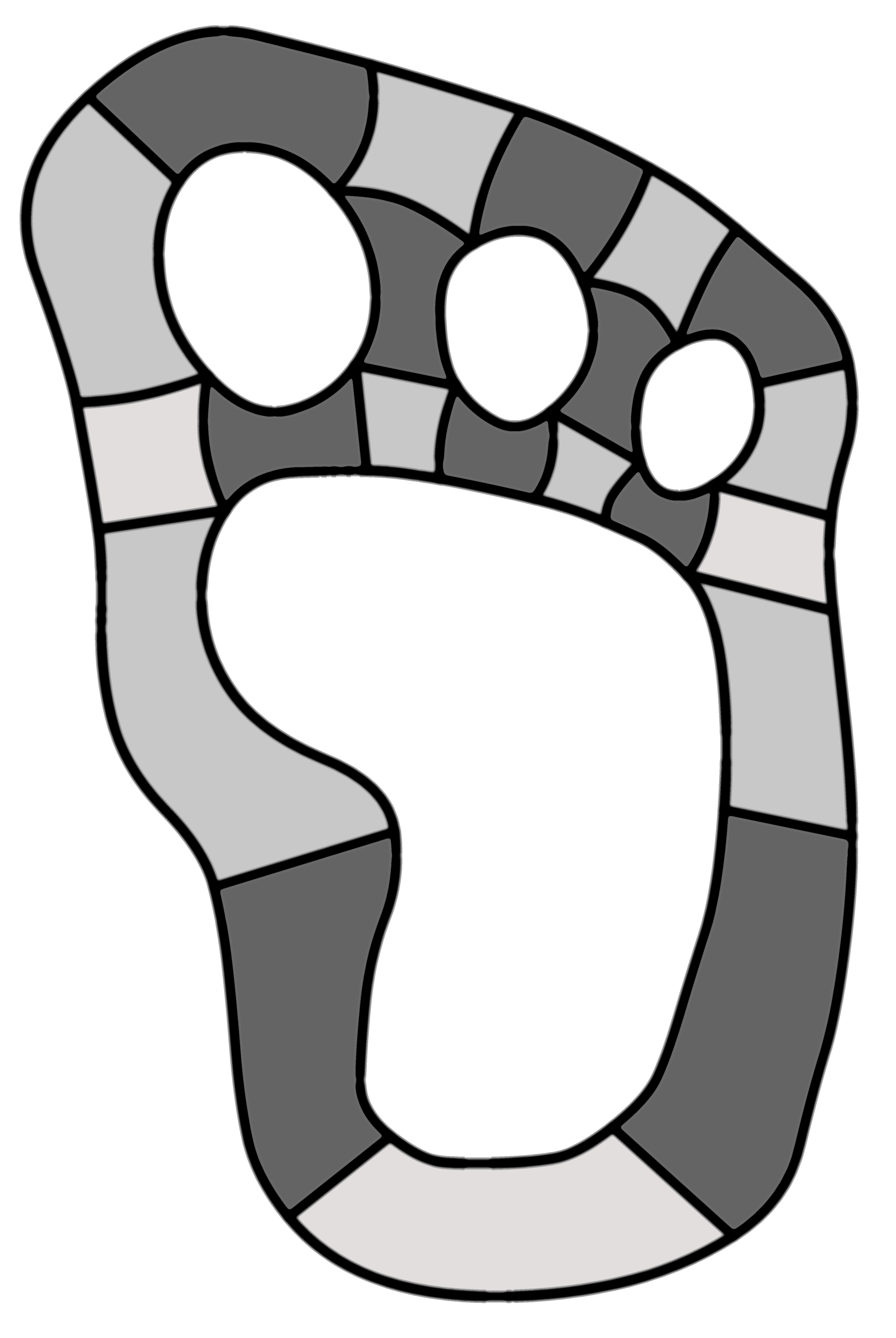
Figure 1: The Yeti footprint

As the domain has a smooth boundary, it is covered by the theory presented within the paper. The domain is decomposed into $21$ patches, which can be seen in Figure 1. Again, we solve for the problem (5.1). For this example, we have to reduce the damping parameter. We choose $\tau=0.25$ and $\sigma=\tfrac{1}{0.2}h^{-2}$. If the multigrid method is used as an iterative scheme, the method suffers from the geometry transformation, so robust convergence is only obtained for 2+2 smoothing steps, cf. Table 6. If the method is used as a preconditioner for a conjugate gradient method, again 1+1 smoothing steps are sufficient for rather good convergence rates, cf. Table 7. Again we observe robustness both in the grid size and the spline degree. Similar iteration counts are obtained for the V-cycle.

$\ell\,\backslash\,p$	2	3	4	5	6	7	8
4	182	194	176	172	182	153	160

Table 6: Multigrid for the Yeti footprint with $2+2$ steps of smoother $L_{h}$ as iterative method

$\ell\,\backslash\,p$	2	3	4	5	6	7	8
4	46	46	45	43	43	40	41
5	48	47	47	46	45	45	44
6	48	49	48	47	47	46	45
7	49	50	49	49	48	47	47

Table 7: Multigrid for the Yeti footprint with $1+1$ steps of smoother $L_{h}$ as preconditioner for conjugate gradient

$\ell\,\backslash\,p$		2	4	6	8
4	# of unknowns	26 368	29 444	32 688	36 100
	W-cycle	2.5 s	4.2 s	9.8 s	17.6 s
	V-cycle	1.8 s	3.1 s	8.0 s	15.0 s
5	# of unknowns	103 936	109 956	116 144	122 500
	W-cycle	10 s	17 s	30 s	48 s
	V-cycle	7 s	12 s	21 s	35 s
6	# of unknowns	412 672	424 580	436 656	448 900
	W-cycle	43 s	66 s	106 s	156 s
	V-cycle	30 s	47 s	74 s	112 s
7	# of unknowns	1 644 544	1 668 228	1 693 080	1 716 100
	W-cycle	185 s	284 s	465 s	712 s
	V-cycle	115 s	187 s	299 s	511 s

Table 8: Multigrid for the Yeti footprint with $1+1$ steps of smoother $L_{h}$ as preconditioner for conjugate gradient

In Table 8, we show actual CPU times required for to execute the numerical tests from Table 7 on a standard personal computer without any parallelization. The CPU times include the setup of the multigrid solver and the solution of the problem (but it excludes the assembling of the stiffness matrix). We observe that for $h$-refinement, the CPU times grow linearly with the number of unknowns. For the spline degree, we observe that the complexity grows less than quadratically with the spline degree. Concluding, we observe that the overall complexity does not exceed $\mathcal{O}(Np^{2})$, the number of non-zero entries of the stiffness matrix.

6 Conclusions

We have introduced a multigrid smoother based on an additive domain decomposition approach and have proven that its convergence rates are robust both in the grid size and the spline degree. The proof only holds if $\mathcal{O}(p)$ smoothing steps are applied, the experiments show however that $1+1$ smoothing steps are enough. So, following the numerical experiments, the proposed smoother yields an optimal multigrid method.

Moreover, we have given a variant of the smoother in Section 4.2, where we could actually prove optimal complexity. The numerical experiments seem to indicate that the original smoother is always superior to that variant, so it is more of theoretical interest.

References

- [1] Y. Bazilevs, L. Beirão da Veiga, J. A. Cottrell, T. J. R. Hughes, and G. Sangalli, Isogeometric analysis: approximation, stability and error estimates for h-refined meshes, Mathematical Models and Methods in Applied Sciences 16 (2006), no. 07, 1031–1090.
- [2] L. Beirão da Veiga, A. Buffa, J. Rivas, and G. Sangalli, Some estimates for h–p–k-refinement in isogeometric analysis, Numerische Mathematik 118 (2011), no. 2, 271–305.
- [3] N. Collier, D. Pardo, L. Dalcin, M. Paszynski, and V. M. Calo, The cost of continuity: A study of the performance of isogeometric finite elements using direct solvers, Computer Methods in Applied Mechanics and Engineering 213–216 (2012), 353–361.
- [4] L. Beirão da Veiga, D. Cho, L. Pavarino, and S. Scacchi, Overlapping Schwarz methods for isogeometric analysis, SIAM Journal on Numerical Analysis 50 (2012), no. 3, 1394–1416.
- [5] , BDDC preconditioners for isogeometric analysis, Mathematical Models and Methods in Applied Sciences 23 (2013), no. 6, 1099–1142.
- [6] L. Beirão da Veiga, L. F. Pavarino, S. Scacchi, O. B. Widlund, and S. Zampini, Isogeometric BDDC preconditioners with deluxe scaling, SIAM Journal on Scientific Computing 36 (2014), no. 3, A1118–A1139.
- [7] M. Dauge, Elliptic boundary value problems on corner domains. Smoothness and asymptotics of solutions, Lecture Notes in Mathematics, 1341. Berlin etc.: Springer-Verlag, 1988.
- [8] , Neumann and mixed problems on curvilinear polyhedra, Integral Equations Oper. Theory 15 (1992), 227 – 261.
- [9] C. de Boor, On calculating with B-splines, Journal of Approximation Theory 6 (1972), no. 1, 50–62.
- [10] M. Donatelli, C. Garoni, C. Manni, S. Serra-Capizzano, and H. Speleers, Symbol-based multigrid methods for Galerkin B-spline isogeometric analysis, SIAM J. Numer. Anal. 55 (2016), no. 1, 31–62.
- [11] M. Floater and E. Sande, Optimal spline spaces of higher degree for l2 n-widths, Journal of Approximation Theory 216 (2017), 1 – 15.
- [12] K. P. S. Gahalaut, J. K. Kraus, and S. K. Tomar, Multigrid methods for isogeometric discretization, Computer Methods in Applied Mechanics and Engineering 253 (2013), 413–425.
- [13] W. Hackbusch, Multi-Grid Methods and Applications, Springer, Berlin, 1985.
- [14] C. Hofer, U. Langer, and S. Takacs, Inexact dual-primal isogeometric tearing and interconnecting methods, (2017), Submitted. https://arxiv.org/abs/1705.04531.
- [15] C. Hofreither, 2017, Private communication.
- [16] C. Hofreither and S. Takacs, Robust multigrid for isogeometric analysis based on stable splittings of spline spaces, SIAM J. on Numerical Analysis 4 (2017), no. 55, 2004–2024.
- [17] C. Hofreither, S. Takacs, and W. Zulehner, A robust multigrid method for isogeometric analysis in two dimensions using boundary correction, Computer Methods in Applied Mechanics and Engineering 316 (2017), 22–42.
- [18] C. Hofreither and W. Zulehner, Spectral analysis of geometric multigrid methods for isogeometric analysis, Numerical Methods and Applications (I. Dimov, S. Fidanova, and I. Lirkov, eds.), Lecture Notes in Computer Science, vol. 8962, Springer International Publishing, 2015, pp. 123–129.
- [19] T. J. R. Hughes, J. A. Cottrell, and Y. Bazilevs, Isogeometric analysis: CAD, finite elements, NURBS, exact geometry and mesh refinement, Computer Methods in Applied Mechanics and Engineering 194 (2005), no. 39-41, 4135–4195.
- [20] S. K. Kleiss, C. Pechstein, B. Jüttler, and S. Tomar, IETI – Isogeometric tearing and interconnecting, Computer Methods in Applied Mechanics and Engineering 247–248 (2012), 201–215.
- [21] J. Necas, Les méthodes directes en théorie des équations elliptiques, Masson, Paris, 1967.
- [22] G. Sangalli and M. Tani, Isogeometric preconditioners based on fast solvers for the Sylvester equation, SIAM J. Sci. Comput 38 (2016), no. 6, A3644–A3671.
- [23] C. Schwab, - and -finite element methods: Theory and applications in solid and fluid mechanics, Numerical Mathematics and Scientific Computation, Clarendon Press, Oxford, 1998.
- [24] S. Takacs, A. Mantzaflaris, et al., G+Smo, http://gs.jku.at/gismo, 2017.
- [25] S. Takacs and T. Takacs, Approximation error estimates and inverse inequalities for B-splines of maximum smoothness, Mathematical Models and Methods in Applied Sciences 26 (2016), no. 07, 1411–1445.