kattributesattributestyleattributestyleld 1
Synthesizing Coupling Proofs of Differential Privacy
Abstract.
Differential privacy has emerged as a promising probabilistic formulation of privacy, generating intense interest within academia and industry. We present a push-button, automated technique for verifying -differential privacy of sophisticated randomized algorithms. We make several conceptual, algorithmic, and practical contributions: (i) Inspired by the recent advances on approximate couplings and randomness alignment, we present a new proof technique called coupling strategies, which casts differential privacy proofs as a winning strategy in a game where we have finite privacy resources to expend. (ii) To discover a winning strategy, we present a constraint-based formulation of the problem as a set of Horn modulo couplings (hmc) constraints, a novel combination of first-order Horn clauses and probabilistic constraints. (iii) We present a technique for solving hmc constraints by transforming probabilistic constraints into logical constraints with uninterpreted functions. (iv) Finally, we implement our technique in the FairSquare verifier and provide the first automated privacy proofs for a number of challenging algorithms from the differential privacy literature, including Report Noisy Max, the Exponential Mechanism, and the Sparse Vector Mechanism.
1. Introduction
As more and more personal information is aggregated into massive databases, a central question is how to safely use this data while protecting privacy. Differential privacy (Dwork et al., 2006) has recently emerged as one of the most promising formalizations of privacy. Informally, a randomized program is differentially private if on any two input databases differing in a single person’s private data, the program’s output distributions are almost the same; intuitively, a private program shouldn’t depend (or reveal) too much on any single individual’s record. Differential privacy models privacy quantitatively, by bounding how much the output distribution can change.
Besides generating intense interest in fields like machine learning, theoretical computer science, and security, differential privacy has proven to be a surprisingly fruitful target for formal verification. By now, several verification techniques can automatically prove privacy given a lightly annotated program; examples include linear type systems (Reed and Pierce, 2010; Gaboardi et al., 2013) and various flavors of dependent types (Barthe et al., 2015; Zhang and Kifer, 2017). For verification, the key feature of differential privacy is composition: private computations can be combined into more complex algorithms while automatically satisfying a similar differential privacy guarantee. Composition properties make it easy to design new private algorithms, and also make privacy feasible to verify.
While composition is a powerful tool for proving privacy, it often gives an overly conservative estimate of the privacy level for more sophisticated algorithms. Verification—in particular, automated verification—has been far more challenging for these examples. However, these algorithms are highly important to verify since their proofs are quite subtle. One example, the Sparse Vector mechanism (Dwork et al., 2009), has been proposed in slightly different forms at least six separate times throughout the literature. While there were proofs of privacy for each variant, researchers later discovered that only two of the proofs were correct (Lyu et al., 2017). Another example, the Report Noisy Max mechanism (Dwork and Roth, 2014), has also suffered from flawed privacy proofs in the past.
1.1. State-of-the-art in Differential Privacy Verification
Recently, researchers have developed techniques to verify private algorithms beyond composition: approximate couplings (Barthe et al., 2016b) and randomness alignment (Zhang and Kifer, 2017).
- Approximate Couplings.:
-
Approximate couplings are a generalization of couplings (Lindvall, 2002) from probability theory. Informally, a coupling models two distributions with a single correlated distribution, while an approximate coupling approximately models the two given distributions. Given two output distributions of a program, the existence of a coupling with certain properties can imply target properties about the two output distributions, and about the program itself.
Approximate couplings are a rich abstraction for reasoning about differential privacy, supporting clean, compositional proofs for many examples beyond the reach of the standard composition theorems for differential privacy. Barthe et al. (2016b) first explored approximate couplings for proving differential privacy, building approximate couplings in a relational program logic apRHL where the rule for the random sampling command selects an approximate coupling. While this approach is quite expressive, there are two major drawbacks: (i) Constructing proofs requires significant manual effort—existing proofs are formalized in an interactive proof assistant—and selecting the correct couplings requires considerable ingenuity. (ii) Like Hoare logic, apRHL does not immediately lend itself to a systematic algorithmic technique for finding invariants, making it a challenging target for automation.
- Randomness Alignment.:
-
In an independent line of work, Zhang and Kifer (2017) used a technique called randomness alignment to prove differential privacy. Informally, a randomness alignment for two distributions is an injection pairing the samples in the first distribution with samples in the second distribution, such that paired samples have approximately the same probability. Zhang and Kifer (2017) implemented their approach in a semi-automated system called LightDP, combining a dependent type system, a custom type-inference algorithm to search for the desired randomness alignments, and a product program construction. Notably, LightDP can analyze standard examples as well as more advanced examples like the Sparse Vector mechanism. While LightDP is an impressive achievement, it, too has a few shortcomings: (i) While randomness alignments can be inferred by LightDP’s sophisticated type inference algorithm, the full analysis depends on a product program construction with manually-provided loop invariants. (ii) Certain examples provable by approximate couplings seem to lie beyond the reach of LightDP. (iii) Finally, the analysis in LightDP is technically complex, involving three kinds of program analysis.
While the approaches seem broadly similar, their precise relation remains unclear. Proofs using randomness alignment are often simpler—critical for automation—while approximate couplings seem to be a more expressive proof technique.
1.2. Our Approach: Automated Synthesis of Coupling Proofs
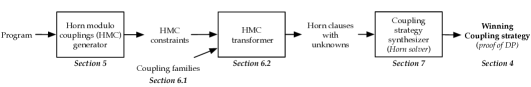
We aim to blend the best features of both approaches—expressivity and automation—enabling fully automatic construction of coupling proofs. To do so, we (i) present a novel formulation of proofs of differential privacy via couplings, (ii) present a constraint-based technique for discovering coupling proofs, and (iii) discuss how to solve these constraints using techniques from automated program synthesis and verification. We describe the key components and novelties of our approach below, and illustrate the overall process in Fig. 1.
Proofs via Coupling Strategies.
The most challenging part of a coupling proof is selecting an appropriate coupling for each sampling instruction. Our first insight is that we can formalize the proof technique as discovering a coupling strategy, which chooses a coupling for each part of the program while ensuring that the couplings can be composed together. A winning coupling strategy proves that the program is differentially private.
To show soundness, we propose a novel, fine-grained version of approximate couplings—variable approximate couplings—where the privacy level can vary depending on the pair of states. We show that a winning coupling strategy encodes a variable approximate coupling of the two output distributions, establishing differential privacy for the program. To encode more complex proofs, we give new constructions of variable approximate couplings inspired by the randomness alignments of Zhang and Kifer (2017).
Horn Modulo Couplings.
To automatically synthesize coupling strategies, we describe winning coupling strategies as a set of constraints. Constraint-based techniques are a well-studied tool for synthesizing loop invariants, rely-guarantee proofs, ranking functions, etc. For instance, constrained Horn clauses are routinely used as a first-order-logic representation of proof rules (Bjørner et al., 2015; Grebenshchikov et al., 2012b). The constraint-based style of verification cleanly decouples the theoretical task of devising the proof rules from the algorithmic task of solving the constraints.
However, existing constraint systems are largely geared towards deterministic programs—it is not clear how to encode randomized algorithms and the differential privacy property. We present a novel system of constraints called Horn modulo couplings (hmc), extending Horn clauses with probabilistic coupling constraints that use first-order relations to encode approximate couplings. hmc constraints can describe winning coupling strategies.
Solving Horn Modulo Couplings Constraints.
Solving hmc constraints is quite challenging, as they combine logical and probabilistic constraints. To simplify the task, we transform probabilistic coupling constraints into logical constraints with unknown expressions. The key idea is that we can restrict coupling strategies to use known approximate couplings from the privacy literature, augmented with a few new constructions we propose in this work.
Our transformation yields a constraint of the form , read as: there exists a strategy such that for all inputs , the program is differentially private. We employ established techniques from synthesis and program verification to solve these simplified constraints. Specifically, we use counterexample-guided inductive synthesis (cegis) (Solar-Lezama et al., 2006) to discover a strategy , and predicate abstraction (Graf and Saïdi, 1997) to prove that is a winning strategy.
Implementation and Evaluation.
We have implemented our technique in the FairSquare probabilistic verification infrastructure (Albarghouthi et al., 2017) and used it to automatically prove -differential privacy of a number of algorithms from the literature that have so far eluded automated verification. For example, we give the first fully automated proofs of Report Noisy Max (Dwork and Roth, 2014), the discrete exponential mechanism (McSherry and Talwar, 2007), and the Sparse Vector mechanism (Lyu et al., 2017).
1.3. Outline and Contributions
After illustrating our technique on a motivating example (§ 2), we present our main contributions.
- •
-
•
We introduce Horn modulo couplings, which enrich first-order Horn clauses with probabilistic coupling constraints. We show how to reduce the problem of proving differential privacy to solving Horn modulo couplings constraints (§ 5).
-
•
We show how to automatically solve Horn modulo couplings constraints by transforming probabilistic coupling constraints into logical constraints with unknown expressions (§ 6).
-
•
We use automated program synthesis and verification techniques to implement our system, and demonstrate its ability to efficiently and automatically prove privacy of a number of differentially private algorithms from the literature (§ 7).
Our approach marries ideas from probabilistic relational logics and type systems with constraint-based verification and synthesis; we compare with other verification techniques (§ 8).
2. Motivation and Illustration
In this section, we demonstrate our verification technique on a concrete example. Our running example is an algorithm from the differential privacy literature called Report Noisy Max (Dwork and Roth, 2014), which finds the query with the highest value in a list of counting queries. For instance, given a database of medical histories, each query in the list could count the occurrences of a certain medical condition. Then, Report Noisy Max would reveal the condition with approximately the most occurrences, adding random noise to protect the privacy of patients.
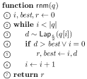
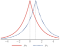
We implement this algorithm in Fig. 2 (top) as the program rnm. Given an array of numeric queries of size , rnm evaluates each query, adds noise to the answer, and reports the index of the query with the largest noisy answer. To achieve -differential privacy (-dp, for short), Laplacian noise is added to the result of each query in the first statement of the while loop. (Fig. 2 (bottom) shows two Laplace distributions.) While the code is simple, proving -dp is anything but—the only existing formal proof uses the probabilistic relational program logic apRHL and was carried out in an interactive proof assistant (Barthe et al., 2016b).
2.1. Proof by approximate coupling, intuitively
Differential privacy is a relational property of programs (also known as a hyperproperty) that compares the output distributions on two different inputs, modeling two hypothetical versions of the private data that should be considered indistinguishable. In the case of rnm, the private data is simply the list of query answers ; we will assume that two input states are similar (also called adjacent) when each query answer differs by at most in the two inputs; formally, , where are copies of in the adjacent states, and .
Adding to the verification challenge, differential privacy is also a quantitative property, often parameterized by a number . To prove -differential privacy, we must show that the probability of any final output is approximately the same in two executions of the program from any two adjacent inputs. The degree of similarity—and the strength of the privacy guarantee—is governed by : smaller values of guarantee more similar probabilities, and yields stronger privacy guarantees. Formally, rnm is -dp if
for every pair of adjacent inputs and , every possible output , and every ,
While it could theoretically be possible to analyze the two executions separately and then verify the inequality, this approach is highly complex. Instead, let us imagine that we step through the two executions side-by-side while tracking the two states. Initially, we have the input states . A deterministic instruction simply updates both states, say to .
Random sampling instructions are more challenging to handle. Since we are considering two sampling instructions, in principle we need to consider all possible pairs of samples in the two programs. However, since we eventually want to show that the probability of some output in the first run is close to the probability of that same output in the second run, we can imagine pairing each result from the first sampling instruction with a corresponding result from the second sampling instruction, with approximately the same probabilities. This pairing yields a set of paired states; intuitively, one for each possible sample. By flowing this set forward through the program—applying deterministic instructions, selecting how to match samples for sampling instructions, and so on—we end up pairing every possible output state in the first execution with a corresponding output state in the second execution with approximately the same probability.
Proving differential privacy, then, boils down to cleverly finding a pairing for each sampling instruction in order to ensure that all paired output states are related in some particular way. For instance, if whenever the first output state has return value its matching state also has return value , then the probability of returning is roughly the same in both distributions.
Approximate Couplings.
This idea for proving differential privacy can be formalized as a proof by approximate coupling, inspired by the proof by coupling technique from probability theory (see, e.g., Lindvall (2002)). An approximate coupling for two probability distributions is a relation attaching a non-negative real number to every pair of linked (or coupled) states . The parameter bounds how far apart the probability of in is from the probability of in : when the two probabilities must be equal, while a larger allows greater differences in probabilities. This parameter may grow as our analysis progresses through the program, selecting approximate couplings for the sampling instructions as we go. If we have two states that have probabilities that are bounded by and we then pair the results from the next sampling instruction with probabilities bounded by , the resulting paired states will have probabilities bounded by . We can intuitively think of as a cost that we need to pay in order to pair up the samples from two sampling instructions.
To make this discussion more concrete, suppose we sample from the two Laplace distributions in Fig. 2 (bottom) in the two runs. This figure depicts the probability density functions (pdf) of two different Laplace distributions over the integers :111For visualization, we use the continuous Laplace distribution; formally, we assume the discrete Laplace distribution. (red; solid) is centered at and (blue; dashed) is centered at . Then, the relation
is a possible approximate coupling for the two distributions, denoted , where the cost depends on the width of the Laplace distributions. The coupling pairs every sample from with the same sample from . These samples have different probabilities—since and are not equal—so the coupling records that the two probabilities are within an multiple of one another.222When is small, this is roughly a factor.
In general, two distributions have multiple possible approximate couplings. Another valid coupling for and is
This coupling pairs each sample from with the sample from . Since is just shifted by , we know that the probabilities of sampling from and from are in fact equal. Hence, each pair has cost and we incur no cost from selecting this coupling.
Concrete Example.
Let us consider the concrete case of rnm with adjacent inputs and , and focus on one possible return value . To prove the probability bound for output , we need to choose couplings for the sampling instructions such that every pair of linked output states has cost , and if the first output is , then so is the second output. In other words, the coupled outputs should satisfy the relation .
In the first iteration, our analysis arrives at the sampling instruction , representing a sample from the Laplace distribution with mean and scale . Since and are apart, we can couple the values of and with the first coupling
By paying a cost , we can assume that ; effectively, applying the coupling as replaces the probabilistic assignments into a single assignment, where the two processes non-deterministically choose a coupled pair of values from . Therefore, the processes enter the same branch of the conditional and always set to the same value—in particular, if , then , as desired. Similarly, in the second iteration, we can select the same coupling and pay . This brings our total cost to and ensures that both processes return the same value —in particular, if then , again establishing the requirement for -dp for output .
This assignment of a coupling for each iteration is an example of a coupling strategy: namely, our simple strategy selects in every iteration. This strategy also applies for more general inputs, but possibly with a different total cost. For instance if we consider larger inputs, e.g., with , we will have to pay in three iterations, and therefore we cannot conclude -dp. Indeed, this strategy only establishes -differential privacy in general, as we pay in each of the loop iterations. Since larger parameters correspond to looser differential privacy guarantees, this is a weaker property. However, Report Noisy Max is in fact -dp for arrays of any length. To prove this stronger guarantee, we need a more sophisticated coupling strategy.
We call coupling strategies that establish -dp winning couplings strategies. Intuitively, the verifier plays a game against the two processes: The processes play by making non-deterministic choices, while the verifier plays by selecting and paying for approximate couplings of sampling instructions, aiming to stay under a “budget” .
2.2. Synthesizing winning coupling strategies
Let us consider a different coupling strategy for rnm. Informally, we will focus on one possible output at a time, and we will only pay non-zero cost in the iteration where may be set to . By paying for just a single iteration, our cost will be independent of the number of iterations . Consider the following winning coupling strategy:
-
(1)
In loop iterations where , select the following coupling (known as the null coupling):
This coupling incurs privacy cost while ensuring that the two samples remain the same distance apart as and .
-
(2)
In iteration , select the following coupling (known as the shift coupling):
Let us explain the idea behind this strategy. In all iterations where , the processes choose two linked values in that differ by at most (since ). So the two processes may take different branches of the conditional, and therefore disagree on the values of and . When , we select the shift coupling to ensure that . Therefore, if is set to , then is set to ; this is because (i) and (ii) will have to be greater than any of the largest values () encountered by the second execution, forcing the second execution to enter the then branch and update . Thus, this coupling strategy ensures that if at the end of the execution, then . Since a privacy cost of is only incurred for the single iteration when , each pair of linked outputs has cost . This establishes -dp of rnm.
Constraint-Based Formulation of Coupling Proofs.
We can view the coupling strategy as assigning a first-order relation
over to every sampling instruction in the program. The vector of variables contains two copies the program variables, along with two logical variables representing the output we are analyzing and the privacy parameter .
Fixing a particular program state , we interpret as a ternary relation over —a coupling of the two (integer-valued) distributions in the associated sampling instruction, where records the cost of this coupling. Effectively, the relation encodes a function that takes the current state of the two processes as an input and returns a coupling.
Finding a winning coupling strategy, then, boils down to finding an appropriate interpretation of the relation . To do so, we generate a system of constraints whose solutions are winning coupling strategies. A solution of encodes a proof of -dp. For instance, our implementation finds the following solution of for rnm (simplified for illustration):
This is a first-order Boolean formula whose satisfying assignments are elements of ; the two conjuncts encode the null and shift coupling, respectively.
Horn Modulo Couplings.
More generally, we work with a novel combination of first-order-logic constraints—in the form of constrained Horn clauses—and probabilistic coupling constraints. We call our constraints Horn modulo couplings (hmc) constraints.
Below, we illustrate the more interesting hmc constraints generated by our system for rnm. Suppose that the unknown relation captures the coupled invariant of the two processes at line number . Just like an invariant for a sequential program encodes the set of reachable states at a program location, the coupled invariant describes the set of reachable states of the two executions (along with privacy cost ) assuming a particular coupling of the sampling instructions.
Informally, a Horn clause is an implication () describing the flow of states between consecutive lines of the program, and constraints on permissible states at each program location. Clause encodes the loop entry condition: if both processes satisfy the loop-entry condition at line 2, then both states are propagated to line 3. Clause encodes the conditions for -dp at the end of the program (line 7): the coupled invariant implies that incurred privacy cost is at most , and if the first process returns , then so does the second process. Clause encodes the effect of selecting the coupling from the strategy at line — is incremented by the privacy cost and are updated to new values , non-deterministically chosen from the coupling provided by the strategy.
Clauses 1–3 are standard constrained Horn clauses, but they are not enough: we need to ensure that encodes a coupling. So, our constraint system also features probabilistic coupling constraints:
The constraint says that if we fix the first argument of to be the current state, the resulting ternary relation is a coupling for the two distributions and .
Solving hmc Constraints.
To solve hmc constraints, we transform the coupling constraints into standard Horn clauses with unknown expressions (uninterpreted functions). To sketch the idea, observe that a strategy can be encoded by a formula of the following form:
This describes a case statement: if the state of the processes satisfies , then select coupling . To find formulas and , we transform solutions of to a formula of the above form, parameterized by unknown expressions. By syntactically restricting to known couplings, we end up with a system of Horn clauses with unknown expressions in and whose satisfying assignments always satisfy the coupling constraints.
Finally, solving a system of Horn clauses with unknown expressions is similar to program synthesis for programs with holes, where we want to find a completion that results in a correct program; here, we want to synthesize a coupling strategy proving -dp. To implement our system, we leverage automated techniques from program synthesis and program verification.
3. Differential Privacy and Variable Approximate Couplings
In this section we define our program model (§ 3.1) and -differential privacy (§ 3.2). We then present variable approximate couplings (§ 3.3), which generalize the approximate couplings of Barthe et al. (2017b); Barthe et al. (2016b) and form the theoretical foundation for our coupling strategies proof method.
3.1. Program Model
Probability Distributions.
To model probabilistic computation, we will use probability distributions and sub-distributions. A function defines a sub-distribution over a countable set if ; when , we call a distribution. We will often write for a subset to mean . We write and for the set of all sub-distributions and distributions over , respectively.
We will use a few standard constructions on sub-distributions. First, the support of a sub-distribution is defined as . Second, for a sub-distribution on pairs , the first and second marginals of , denoted and , are sub-distributions in and :
We will use to denote a distribution family, which is a function mapping every parameter in some set of distribution parameters to a sub-distribution in .
Variables and Expressions.
We will work with a simple computational model where programs are labeled graphs. First, we fix a set of program variables, the disjoint union of input variables and local variables . Input variables model inputs to the program and are never modified—they can also be viewed as logical variables. We assume that a special, real-valued input variable contains the target privacy level. The set of local variables includes an output variable , representing the value returned by the program. We assume that each variable has a type , e.g., the Booleans , the natural numbers , or the integers .
We will consider several kinds of expressions, built out of variables. We will fix a collection of primitive operations; for instance, arithmetic operations and , Boolean operations , etc. We shall use to denote expressions over variables , to denote Boolean expressions over , and to denote input expressions over . We consider a set of distribution expressions modeling primitive, built-in distributions. For our purposes, distribution expressions will model standard distributions used in the differential privacy literature; we will detail these when we introduce differential privacy below. Distribution expressions can be parameterized by standard expressions.
Finally, we will need three kinds of basic program statements . An assignment statement stores the value of into the variable . A sampling statement takes a fresh sample from the distribution and stores it into . Finally, an assume statement does nothing if is true, otherwise it filters out the execution (fails to terminate).
Programs.
A program is a directed graph where nodes represent program locations, directed edges connect pairs of locations, and each edge is labeled by a statement . There is a distinguished entry location , representing the first instruction of the program, and a return location . We assume all locations in can reach by following edges in .
![[Uncaptioned image]](/html/1709.05361/assets/x4.png)
Our program model is expressive enough to encode the usual conditionals and loops from imperative languages—e.g., consider the program on the right along with its graph representation. All programs we consider model structured programs, e.g., there is no control-flow non-determinism.
Expression Semantics.
A program state is a map assigning a value to each variable in ; let denote the set of all possible states. Given variable , we use to denote the value of in state . Given constant , we use to denote the state but with variable mapped to . The semantics of an expression is a function from a state to an element of some type . For instance, the expression in state is interpreted as . A distribution expression is interpreted as a distribution family , mapping a state in to a distribution over integers; for concreteness we will only consider distributions over integers, but extending to arbitrary discrete distributions is straightforward. We will often write to denote , for simplicity.
Program Semantics.
We can define semantics of a program as the aggregate of all its traces. A trace through is a finite sequence of statements such that the associated edges edges form a directed path through the graph. A maximal trace has edges corresponding to a path from to . We use to denote the set of all maximal traces through . A trace represents a sequence of instructions to be executed, so we define as a distribution family from states to sub-distributions over states. Assignments and sampling statements are given the expected semantics, and an statement yields the all-zeros sub-distribution if the input state does not satisfy the guard . We can now define the semantics of a full program as
where the sum adds up output sub-distributions from each trace. We will assume is terminating; in particular, the sub-distributions sum to a proper distribution.
3.2. Differential Privacy
Differential privacy is a quantitative, statistical notion of data privacy proposed by Dwork et al. (2006); we reformulate their definition in our program model. We will fix an adjacency relation on input states modeling which inputs should lead to similar outputs. Throughout, we implicitly assume (i) for all , , and (ii) for all and every , . In other words, in adjacent states may take any positive value, as long as it is equal in both states.
Definition 3.1 (Dwork et al. (2006)).
A program is -differentially private with respect to an adjacency relation iff for every and output ,
where , , and .
Dwork et al. (2006) originally defined differential privacy in terms of sets of outputs rather than single outputs. Def. 3.1 is equivalent to their notion of -differential privacy and is more convenient for our purposes, as we will often prove privacy by focusing on one output at at time.
We will consider two primitive distributions that are commonly used in differentially private algorithms: the (discrete) Laplace and exponential distributions. Both distributions are parameterized by two numbers, describing the spread of the distribution and its center.
Definition 3.2.
The Laplace distribution family is a function with two parameters, and . We use to denote the distribution over where , for all . We call the scale of the distribution and the mean of the distribution.
Definition 3.3.
The exponential distribution family is a function with two parameters, and . We use to denote the distribution over where for all , and for all .
We will use distribution expressions and to represent the respective Laplace/exponential distribution interpreted in a given state. We assume that every pair of adjacent states satisfies for every appearing in distribution expressions.
3.3. Variable Approximate Couplings
We are now ready to define the concept of a variable approximate coupling, which we will use to establish -dp of a program. A variable approximate coupling of two distributions and can be viewed as two distributions on pairs, each modeling one of the original distributions. Formally:
Definition 3.4 (Variable approximate couplings).
Let and . Let be a relation. We write for the projection of to the first two components. We say that is a variable approximate coupling of and —denoted —if there exist two witness sub-distributions and such that:
-
(1)
and ,
-
(2)
, and
-
(3)
for all , we have .
We will call these the marginal conditions, the support conditions, and the distance conditions respectively. We will often abbreviate “variable approximate coupling” as simply “coupling”.
To give some intuition, the first point states that models the first distribution and is a lower bound on the second distribution—the inequality means that for every . Informally, since the definition of differential privacy (Def. 3.1) is asymmetric, it is enough to show that the first distribution (which we will model by ) is less than a lower bound of the second distribution (which we will model by ). The second point states that every pair of elements with non-zero probability in or must have at least one cost. Finally, the third point states that is approximately upper bounded by ; the approximation is determined by a cost at each pair.
Our definition is a richer version of -lifting, an approximate coupling recently proposed by Barthe et al. (2017b) for verifying differential privacy. The main difference is our approximation level may vary over the pairs , hence we call our approximate coupling a variable approximate coupling. When all approximation levels are the same, our definition recovers the existing definition of -lifting.333More precisely, -lifting. Variable approximate couplings can give more precise bounds when comparing events in the first distribution to events in the second distribution.
Now, -dp holds if we can find a coupling of the output distributions from adjacent inputs.
Lemma 3.5 (-dp and couplings).
A program is -dp with respect to adjacency relation if for every and , there is a coupling with
where .
We close this section with some examples of specific couplings for the Laplace and exponential distributions proposed by Barthe et al. (2016b).
Definition 3.6 (Shift coupling).
Let , , and , and define the relations
Then we have the following shift coupling for the Laplace distribution:
If , we have the following shift coupling for the exponential distribution:
Intuitively, these couplings relate each sample from the first distribution with the sample from the second distribution. The difference in probabilities for these two samples depends on the shift and the difference between the means .
If we set above, the coupling cost is and we have the following useful special case.
Definition 3.7 (Null coupling).
Let , , and define the relation:
Then we have the following null couplings:
Intuitively, these couplings relate pairs of samples that are at the same distance from their respective means —the approximation level is since linked samples have the same probabilities under their respective distributions.
4. Coupling Strategies
In this section, we introduce coupling strategies, our proof technique for establishing -dp.
4.1. Formalizing Coupling Strategies
Roughly speaking, a coupling strategy picks a coupling for each sampling statement.
Definition 4.1 (Coupling strategies).
Let Stmts be the set of all sampling statements in a program ; recall that our primitive distributions are over the integers . A coupling strategy for is a map from to couplings in , such that for a statement and states , the relation forms a coupling
Example 4.2.
Recall our simple coupling strategy for Report Noisy Max in § 2.1. For the statement , and every pair of states where , the strategy returned the coupling .
To describe the effect of a coupling strategy on two executions from neighboring inputs, we define a coupled postcondition operation. This operation propagates a set of pairs of coupled states while tracking the privacy cost from couplings selected along the execution path.
Definition 4.3 (Coupled postcondition).
Let be a coupling strategy for . We define the coupled postcondition as a function , mapping and a statement to a subset of :
This operation can be lifted to operate on sequences of statements in the standard way: when the trace begins with , we define ; when is the empty trace, .
Intuitively, on assignment statements updates every pair of states using the semantics of assignment; on assume statements, only propagates pairs of states satisfying ; on sampling statements, updates every pair of states by assigning the variables with every possible pair from the coupling chosen by , updating the incurred privacy costs.
Example 4.4.
Consider a simple program:
Let the adjacency relation and let be a coupling strategy. Since there is only a single variable and is fixed to , we will represent the states of the two processes by and , respectively. Then, the initial set of coupled states is the set . First, we compute This results in a set , since adding 10 to both variables does not change the fact that . Next, we compute Suppose that the coupling strategy maps every pair of states to the coupling . Then,
While a coupling strategy restricts the pairs of executions we must consider, the executions may still behave quite differently—for instance, they may take different paths at conditional statements or run for different numbers of loop iterations, etc. To further simplify the verification task we will focus on synchronizing strategies only, which ensure that the guard in every instruction takes the same value on coupled pairs, so both coupled processes follow the same control-flow path through the program.
Definition 4.5 (Synchronizing coupling strategies).
Given a trace , let denote the prefix of and let denote the empty trace that simply returns the input state. A coupling strategy is synchronizing for and iff for every and , we have .
Requiring synchronizing coupling strategies is a certainly a restriction, but not a serious one for proving differential privacy. By treating conditional statements as monolithic instructions, the only potential branching we need to consider comes from loops. Differentially private algorithms use straightforward iteration; all examples we are aware of can be encoded with for-loops and analyzed synchronously. (§ 7 provides more details about how we handle branching.)
4.2. Proving Differential Privacy via Coupling Strategies
Our main theoretical result shows that synchronizing coupling strategies encode couplings.
Lemma 4.6 (From strategies to couplings).
Suppose is synchronizing for and . Let , and let be such that for all . Then we have a coupling where .
Proof.
(Sketch) By induction on the length of the trace .∎
There may be multiple sampling choices that yield the same coupled outputs ; the coupling must assign a cost larger than all associated costs in the coupled post-condition. By Lem. 3.5, if we can find a coupling for each possible output such that with cost at most , then we establish -differential privacy. We formalize this family of coupling strategies as a winning coupling strategy.
Theorem 4.7 (Winning coupling strategies).
Fix program and adjacency relation . Suppose that we have a family of coupling strategies such that for every trace and , is synchronizing for and
Then is -differentially private. (We could change to above, since in .)
5. Horn Clauses Modulo Couplings
So far, we have seen how to prove differential privacy by finding a winning coupling strategy. In this section we present a constraint-based formulation of winning coupling strategies, paving the way to automation.
5.1. Enriching Horn clauses with Coupling Constraints
Constrained Horn clauses are a standard tool for logically encoding verification proof rules (Bjørner et al., 2015; Grebenshchikov et al., 2012b). For example, a set of Horn clauses can describe a loop invariant, a rely-guarantee proof, an Owicki-Gries proof, a ranking function, etc. Since our proofs—winning coupling strategies—describe probabilistic couplings, our Horn clauses will involve a new kind of probabilistic constraint.
Horn Clauses.
We assume formulas are interpreted in some first-order theory (e.g., linear integer arithmetic) with a set of uninterpreted relation symbols. A constrained Horn clause , or Horn clause for short, is a first-order logic formula of the form
where:
-
•
each relation is of arity equal to the length of the vector of variables ;
-
•
is an interpreted formula over the first-order theory (e.g., );
-
•
the left-hand side of the implication () is called the body of ; and
-
•
, the head of , is either a relation application or an interpreted formula .
We will allow interpreted formulas to contain disjunctions. For clarity of presentation, we will use to denote implications in an interpreted formula, and to denote the implication in a Horn clause. All free variables are assumed to be universally quantified, e.g., means . For conciseness we often write to denote the relation application , where is the vector of variables .
Semantics.
We will write for a set of clauses . Let be a graph over relation symbols such that there is an edge iff appears in the body of some clause and appears in its head. We say that is recursive iff has a cycle. The set is satisfiable if there exists an interpretation of relation symbols as relations in the theory such that every clause is valid. We say that satisfies (denoted ) iff for all , is valid (i.e., equivalent to true), where is with every relation application replaced by .
The next example uses Horn clauses to prove a simple Hoare triple for a standard, deterministic program. For a detailed exposition of Horn clauses in verification, we refer to the excellent survey by Bjørner et al. (2015).
| precondition | ||||
| loop entry | ||||
| loop body | ||||
| loop exit | ||||
| postcondition |
Example 5.1.
Consider the simple program and its graph representation in Fig. 3. Suppose we want to prove the Hoare triple . We generate the Horn clauses shown in Fig. 3, where relations denote the Hoare-style annotation at location of . Each clause encodes either the pre/postcondition or the semantics of one of the program statements.
Notice that the constraint system is recursive. Intuitively, captures all reachable states at location ; relation encodes an inductive loop invariant that holds at the loop head. We can give a straightforward reading of each clause. For instance, states that if is reachable at location , then must be reachable at location ; stipulates that all states reachable at location 5 must be such that , i.e., satisfy the postcondition.
One possible satisfying assignment to these constraints is for . Applying to results in , the loop invariant. We can interpret and under :
Observe that all are valid, establishing validity of the original Hoare triple.
Horn Clauses Modulo Coupling Constraints.
We now enrich Horn clauses with a new form of constraint that describes couplings between pairs of distributions; we call the resulting constraints Horn modulo couplings (hmc).
Definition 5.2 (Coupling constraints).
Suppose we have a relation of arity for some , and suppose we have two distribution families and . A coupling constraint is of the form:
An interpretation satisfies such a constraint iff for every consistent assignment to the variables , , , we have where is defined as . In other words, is the ternary relation resulting from fixing the first components of to . Note that the vectors may share variables.
Example 5.3.
Consider the simple coupling constraint where is a positive constant. A simple satisfying assignment is the null coupling from Def. 3.7:
Effectively, says: for any values of , the relation is a coupling such that .
Example 5.4.
For a simpler example, consider the constraint where is a positive constant. A satisfying assignment to this constraint is: since the two distributions are the same for any value of variable . Another possible satisfying assignment is , by the shift coupling (Def. 3.6).
tensy init tensy dpriv
tensy assign
tensy assume tensy assume-s
tensy strat tensy couple
We use to denote the vector but with variables and replaced by their primed versions, and .
5.2. Generating Horn clauses from Programs
For a program , we generate clauses specifying a winning coupling strategy ; as we saw in Thm. 4.7, a winning coupling strategy implies -differential privacy. A winning coupling strategy ensures that the coupled postcondition satisfies certain conditions for every trace . We thus generate a set of constraints whose solutions capture all sets . Since the set is potentially infinite (due to loops), we generate a recursive system of constraints. Rather than find a coupling strategy separately for each possible output value , we will parameterize our constraints by a logical variable representing a possible output.
Invariant and Strategy Relations.
Our generated constraints mention two unknown relations.
-
•
encodes the coupled invariant at location in the program. This relation captures the set of coupled states for traces that begin at location and end at location . The first-order variables model two copies of program variables for the two executions of , tagged with subscript or , respectively, along with the logical variable representing a possible return value in . The variable models the accumulated cost for the particular coupled states and program location.
-
•
encodes the coupling strategy for sampling statement . If the values of model two program states, encodes a coupling between the distributions in .
Constraint Generation.
Given a program and adjacency relation , the rules in Fig. 4 define a set of constraints. The rule couple generates a coupling constraint for a sampling statement; all other rules generate standard constrained Horn clauses.
Before walking through the rules, we first set some notation. We use (resp. ) to denote with all its variables tagged with subscript (resp. ). As is standard, we assume there is a one-to-one correspondence between expressions in our language and our first-order theory, e.g., if is and is of type , then we treat as the constraint in the theory of linear integer arithmetic. We assume that the adjacency relation is a formula in our first-order theory. Finally, technically there are two distinct input variables and representing the target privacy level. Since these variables are assumed to be equal in any two adjacent states, we will simply use a single variable in the constraints.
Now, we take a closer look at the constraint generation rules. The first two rules describe the initial and final states: the rule init specifies that the invariant at contains all adjacent states and is . The rule dpriv states that the invariant at satisfies the -dp conditions in Thm. 4.7 for every return value and every .
The next three rules describe the coupled postcondition for deterministic statements. The rule assign encodes the effect of executing in the two executions of the program. Primed variables, e.g., , to denote the modified (new) value of after assignment. The rule assume encodes effects of assume statements, and assume-s ensures both processes are synchronized at assume statements.
The last two rules encode sampling statements. The rule strat generates a clause that uses the coupling encoded by to constrain the values of and and increments the privacy cost by . The rule couple generates a coupling constraint specifying that encodes a coupling of the distributions in the two executions. We interpret the distribution expressions as distribution families, parameterized by the state.
Example 5.5.
For illustration, let us walk through the constraints generated for the simple program from Ex. 4.4, reproduced below. Assume the adjacency relation is , and let the vector contain the variables . We write for (as described at the bottom of Fig. 4). Then, the following constraints are generated by the indicated rules from Fig. 4.
| init | |||
| assign | |||
| strat | |||
| dpriv | |||
| couple |
The relation describes the coupling for the single sampling statement.
Soundness.
To connect our constraint system to winning coupling strategies, the main soundness lemma states that a satisfying assignment of encodes a winning coupling strategy.
Lemma 5.6.
Let , where is generated for a program and adjacency relation . Define a family of coupling strategies for by
for every sampling statement in and every pair of states , where replaces each tagged program variable in with the value in and respectively, and sets the output variable to . Then, is a winning coupling strategy.
Theorem 5.7 (Soundness of constraints).
Let be a system of constraints generated for program and adjacency relation , as per Fig. 4. If is satisfiable, then is -differentially private.
6. Parameterized Coupling Families
In this section, we demonstrate how to transform the probabilistic coupling constraints into more standard logical constraints. We introduce parameterized families of couplings (§ 6.1) and then show how to use them to eliminate coupling constraints (§ 6.2).
6.1. Coupling families
Since coupling strategies select couplings for distribution expressions instead of purely mathematical distributions, it will be useful to consider couplings between two families of distributions , parametrized by variables, rather than just between two concrete distributions.
Definition 6.1 (Coupling families).
Let be two distribution families with distribution parameters in some set . Then, a coupling family for and assigns a coupling
for all , where is a precondition on the parameter combinations.
We use square brackets to emphasize the distribution parameters.
Besides distribution parameters—which model the state of the distributions—couplings can also depend on logical parameters independent of the state. We call this second class of parameters coupling parameters. Table 1 lists the selection of couplings we discuss in this section along with their preconditions and coupling parameters; the distribution parameters are indicated by the square brackets.
Null and shift coupling families.
In § 3, we saw two examples of couplings for the Laplace and Exponential distributions: the shift coupling (Def. 3.6) and the null coupling (Def. 3.7). These couplings are examples of coupling families in that they specify a coupling for a family of distributions. For instance, the Laplace distribution has the mean value as a distribution parameter; we will write instead of when we want to emphasize this dependence.444Properly speaking should be considered a parameter as well. To reduce notation, we will suppress this dependence and treat as a constant for this section. The null and shift coupling families couple the distribution families for any two . For example, for a fixed , we have the shift coupling , where . Notice that is a coupling parameter; depending on what we set it to, we get different couplings.
In the case of the exponential distribution, the shift coupling family couples the families and under the precondition that .
| Name | Distribution family | Precondition | Coupling family | Coupling params. |
|---|---|---|---|---|
| Null (Lap) | – | – | ||
| Shift (Lap) | – | |||
| Choice (Lap) | ||||
| Null (Exp) | – | – | ||
| Shift (Exp) |
Choice coupling.
We will also use a novel coupling construction, the choice coupling, which allow us to combine two couplings, using a predicate on the first sample space to decide which coupling to apply. If the two couplings satisfy a non-overlapping condition, the result is again a coupling. This construction is inspired by ideas from Zhang and Kifer (2017), who demonstrate how the pairing between samples (randomness alignment) can be selected depending on the result of the first sample. These richer couplings can simplify privacy proofs (and hence solutions to invariants in our constraints), in some cases letting us construct a single proof that works for all possible output values instead of building a different proof for each output value.
Lemma 6.2 (Choice coupling).
Let , be two sub-distributions, and let be a predicate on . Suppose that there are two couplings and , and suppose that satisfy the following non-overlapping condition: for every pair and , and do not both hold. We abbreviate the non-overlapping condition as . In other words, there is no element that is related under to an element in and related under to an element not in . Then the following relation
is a coupling
Proof.
Let be witnesses for the coupling , and let be witnesses for the coupling . Then we can define witnesses for the choice coupling :
The support and distance conditions follow from the support and distance conditions for and . The first marginal condition for follows from the first marginal conditions for and , while the second marginal condition for follows from the second marginal conditions for and combined with the non-overlapping condition on , , and . ∎
We can generalize a choice coupling to a coupling family. Suppose we have two coupling families for some distribution families , , then we can generate a coupling family whose coupling parameters are the predicate and the parameters of the two families. (Note that could also have parameters.) In the example below, and in Table 1, we give one possible choice coupling for the Laplace distribution. An analogous construction applies for the exponential distribution
Example 6.3.
Consider the following two coupling families for the Laplace distribution family: the shift coupling and the null coupling . Then, we have the coupling family
under the precondition . The parameters of this coupling family are the predicate and the parameter of . For one possible instantiation, let be the predicate and let . Then if , the non-overlapping condition holds and is a coupling.
6.2. Transforming Horn clauses
Now, we can transform hmc constraints and eliminate coupling constraints by restricting solutions of coupling constraints to use the previous coupling families. We model coupling parameters and the logic of the coupling strategy by Horn clauses with uninterpreted functions.
Horn clauses with uninterpreted functions.
Recall our Horn clauses may mention uninterpreted relation symbols . We now assume an additional set of uninterpreted function symbols, which can appear in interpreted formulas in the body/head of a clause . A function symbol of arity can be applied to a vector of variables of length ; for example, consider the clause
In addition to mapping each relation symbol to a relation, an interpretation now also maps each function symbol to a function definable in the theory—intuitively, an expression. We say that iff is valid for all , where also replaces every function application by .
Example 6.4.
To give an intuition for the semantics, consider the two simple clauses:
A possible satisfying assignment maps to the formula (ensuring that the first clause is valid) and to the expression (ensuring that the second clause is valid).
Roughly, we can view the problem of solving a set of Horn clauses as solving a formula of the form : Find an interpretation of and such that is valid. In our setting, will correspond to pieces of the coupling strategy and will be the invariants showing that the coupling strategy establishes differential privacy.
Transforming coupling constraints.
To transform coupling constraints into Horn clauses with uninterpreted functions, we encode each coupling family as a first-order formula, , along with its precondition. The encodings for the families we consider from Table 1 are shown in Fig. 5, where is a fresh nullary (constant) uninterpreted function that is shared between the encoding of a family and its precondition. Similarly, is a fresh uninterpreted function ranging over Booleans, representing a predicate.
With the encodings of coupling families, we are ready to define the transformation.
Definition 6.5 (Coupling constraint transformer).
Suppose we have a coupling constraint
Suppose we have a set of possible coupling families for . We transform the coupling constraint into the following set of Horn clauses, where we use to denote the pair of Horn clauses and , and we use to denote a fresh uninterpreted function with range :
Without loss of generality, we assume that variables do not appear in .
Intuitively, the first clause selects which of the couplings we pick, depending on the values . The remaining clauses ensure that whenever we pick a coupling , we satisfy its precondition.
Example 6.6.
Recall our Report Noisy Max example from § 2. There, we encoded the single sampling statement using the following coupling constraint:
Suppose we take the null and shift coupling families for Laplace as our possible couplings. Our transformation produces:
We omit clauses enforcing the trivial precondition () for these coupling families.
The first conjunct on the left encodes application of the null coupling; the second conjunct encodes the shift coupling. The unknowns are the function and the constant function . As we sketched in § 2, our tool discovers the interpretation for and the constant for , where denotes the expression that is if is true and otherwise.
The following theorem formalizes soundness of our transformation.
Theorem 6.7 (Soundness of transformation).
Let be a set of Horn clauses with coupling constraints. Let be the set with coupling constraints replaced by Horn clauses, as in Def. 6.5. Then, if is satisfiable, is satisfiable.
7. Implementation and Evaluation
We now describe the algorithms we implement for solving Horn clauses, detail our implementation, and evaluate our technique on well-known algorithms from the differential privacy literature.
7.1. Solving Horn clauses with Uninterpreted Functions
Solving Horn clauses with uninterpreted functions is equivalent to a program synthesis/verification problem, where we have an incomplete program with holes and we want to fill the holes to make the program satisfy some specification. In our implementation we employ a counterexample-guided inductive synthesis (cegis) (Solar-Lezama et al., 2006) technique to propose a solution for the uninterpreted functions , and a fixed-point computation with predicate abstraction (Graf and Saïdi, 1997) to verify if the Horn clauses are satisfiable for the candidate interpretation of . Since these techniques are relatively standard in the program synthesis literature, we describe our solver at a high level in this section.
Synthesize–Verify Loop.
Algorithm solve (Fig. 6) employs a synthesize–verify loop as follows:
- Coupling Strategy Synthesis.:
-
In every iteration of the algorithm, the set of clauses are unrolled into a set of clauses , a standard technique in Horn-clause solving roughly corresponding to unrolling program loops up to a finite bound—see, for example, the algorithm of McMillan and Rybalchenko (2013). We assume that there is a single clause whose head is not a relation application—we call it the query clause. The unrolling starts with clause , and creates a fresh copy of every clause whose head is a relation that appears in the body of , and so on, recursively, up to depth . For an example, consider the following three clauses: and . If we unroll these clauses up to , we get the following clauses: (i) , (ii) , and (iii) , where are fresh relation symbols (copies of ).
Once we have non-recursive clauses , we can construct a formula of the form
where and are the function and relation symbols appearing in the unrolled clauses. Since are non-recursive, we can rewrite them to remove the relation symbols. This is a standard encoding in Horn clause solving that is analogous to encoding a loop-free program as a formula—as in VC generation and bounded model checking—and we do not detail it here. We thus transform into a constraint of the form which can be solved using program synthesis algorithms (recall that variables are implicitly universally quantified). Specifically, for synth, we employ a version of the symbolic synthesis algorithm due to Gulwani et al. (2011). The synthesis phase generates an interpretation of the function symbols, a winning coupling strategy that proves -dp for adjacent inputs that terminate in iterations.
- Coupling Strategy Verification.:
-
This second phase verifies whether the synthesized strategy is indeed a winning coupling strategy for all pairs of adjacent inputs by checking if is satisfiable. That is, we plug in the synthesized values of into , resulting in a set of Horn clauses with no uninterpreted functions—only invariant relation symbols —which can be solved with a fixed-point computation. The result of verify could be sat, unsat, or unknown, due to the undecidability of the problem. If the result is sat, then we know that encodes a winning coupling strategy and we are done. Otherwise, we try unrolling further.
While there are numerous Horn-clause solvers available, we have found that they are unable to handle the clauses we encountered. We thus implemented a custom solver that uses predicate abstraction. We detail our implementation and rationalize this decision below.
7.2. Implementation Details
We have implemented our approach by extending the FairSquare probabilistic verifier (Albarghouthi et al., 2017). Our implementation takes a program in a simple probabilistic language with integers and arrays over integers. An adjacency relation is provided as a first-order formula over input program variables. The program is then translated into a set of Horn clauses over the combined theories of linear real/integer arithmetic, arrays, and uninterpreted functions.
Instantiations of the Synthesizer (synth).
To find an interpretation of functions , our synthesis algorithm requires a grammar of expressions to search through. Constant functions can take any integer value. In the case of Boolean and -valued functions, we instantiate the synthesizer with a grammar over Boolean operations, e.g., or , where and can be replaced by variables or numerical expressions over variables. In all of our benchmarks, we find that searching for expressions with asts of depth 2 is sufficient to finding a winning coupling strategy.
Instantiations of Predicate Abstraction (verify).
To compute invariants , we employ predicate abstraction (Graf and Saïdi, 1997). In our initial experiments, we attempted to delegate this process to existing Horn clause solvers. Unfortunately, they either diverged or could not handle the theories we use.555Duality (McMillan and Rybalchenko, 2013), which uses tree interpolants, diverged even on the simplest example. This is due to the interpolation engine not being optimized for relational verification; for instance, in all examples we require invariants containing multiple predicates of the form or , where and are copies of the same variable. SeaHorn (Gurfinkel et al., 2015), hsf (Grebenshchikov et al., 2012a), and Eldarica (Hojjat et al., 2012) have limited or no support for arrays, and could not handle our benchmarks. We thus built a Horn clause solver on top of the Z3 smt solver and instantiated it with a large set of predicates Preds over a rich set of templates over pairs of variables. The templates are of the form: , , , . By instantiating with program variables and with constants, we generate a large set of predicates. We also use the predicates appearing in assume statements. To track the upper bound on , we use a class of predicates of the form that model every increment to the privacy cost, where is the scale parameter in the th sampling statement in the program ( or ), and is instantiated as an expression of the cost of the chosen couplings for the th statement, potentially multiplied by a positive program variable if it occurs in a loop. For instance, if we have the shift coupling, we instantiate with ; if we use the null coupling, is 0. We use all possible combinations of and eliminate any non-linear predicates (see more below).
Since our invariants typically require disjunctions we employ boolean predicate abstraction, an expensive procedure requiring exponentially many smt calls in the size of the predicates in the worst case. To do so efficiently, we use the AllSMT algorithm of Lahiri et al. (2006), as implemented in the MathSAT5 smt solver (Cimatti et al., 2013).
Handling Non-linearity.
Observe that in the definition of shift couplings (Def. 3.6), the parameter is multiplied by an expression, resulting in a non-linear constraint (a theory that is not well-supported by smt solvers, due to its complexity). To eliminate non-linear constraints, we make the key observation that it suffices to set to 1: Since all constraints involving are summations of coefficients of , we only need to track the coefficients of .
Handling Conditionals.
Winning coupling strategies (Thm. 4.7) assume synchronization at each conditional statement. In our implementation, we only impose synchronization at loop heads by encoding conditional code blocks (with no sampling statements) as monolithic instructions, as in large-block encoding (Beyer et al., 2009). This enables handling examples like Report Noisy Max (§ 2), where the two processes may not enter the same branch of the conditional under the strategy.
7.3. Differentially Private Algorithms.
For evaluation, we automatically synthesized privacy proofs for a range of algorithms from the differential privacy literature. The examples require a variety of different kinds of privacy proofs. Simpler examples follow by composition, while more complex examples require more sophisticated arguments. Fig. 7 shows the code for three of the more interesting algorithms, which we discuss below; Table 2 presents the full collection of examples.
fun ExpMech() while do if then return fun NumericSparseN() while do if then return
Two-Level Counter (SmartSum).
The SmartSum algorithm (Chan et al., 2011; Dwork et al., 2010) was designed to continually publish aggregate statistics while maintaining privacy—for example, continually releasing the total number of visitors to a website. Suppose that we have a list of inputs , where denotes the total number of visitors in hour . SmartSum releases a list of all running sums: , . Rather than adding separate noise to each or adding separate noise to each running sum—which would provide weak privacy guarantees or inaccurate results—SmartSum chunks the inputs into blocks of size and adds noise to the sum of each block. Then, each noisy running sum can be computed by summing several noised blocks and additional noise for the remaining inputs. By choosing the block size carefully, this approach releases all running sums with less noise than more naïve approaches, while ensuring -dp.
Discrete Exponential Mechanism (ExpMech).
The exponential mechanism (McSherry and Talwar, 2007) is used when (i) the output of an algorithm is non-numeric or (ii) different outputs have different utility, and adding numeric noise to the output would produce an unusable answer, e.g., in the case of an auction where we want to protect privacy of bidders (Dwork and Roth, 2014). ExpMech takes a database and a quality score (utility function) as input, where the quality score maps the database and each element of the range to a numeric score. Then, the algorithm releases the element with approximately the highest score. We verified a version of this algorithm that adds noise drawn from the exponential mechanism to each quality score, and then releases the element with the highest noisy score. This implementation is also called the one-sided Noisy Arg-Max (Dwork and Roth, 2014).
Sparse Vector Mechanism (NumericSparseN).
The Sparse Vector mechanism (also called NumericSparse in the textbook by Dwork and Roth (2014)) is used in scenarios where we would like to answer a large number of numeric queries while only paying for queries with large answers. To achieve -dp, NumericSparseN releases the noised values of the first queries that are above some known threshold , while only reporting that other queries are below the threshold, without disclosing their values.
Specifically, NumericSparseN takes a list of numeric queries and numeric threshold . Each query is assumed to be -sensitive—its answer may differ by at most on adjacent databases. The threshold is assumed to be public knowledge, so we can model it as being equal in adjacent inputs. The Sparse Vector mechanism adds noise to the threshold and then computes a noisy answer for each query. When the algorithm finds a query where the noisy answer is larger than the noisy threshold, it records the index of the query. It also adds fresh noise to the query answer, and records the (freshly) noised answer as well. When the algorithm records queries or runs out of queries, it returns the final list of indices and answers.
The privacy proof is interesting for two reasons. First, applying the composition theorem of privacy does prove privacy, but with an overly conservative level of that depends on the number of queries. A more careful proof by coupling shows that the privacy level depends only on the number of above threshold queries, potentially a large saving if most of the queries are below threshold. Second, adding fresh noise when estimating the answer of above threshold queries is critical for privacy—it is not private to reuse the noisy answer of the query from checking against the noisy threshold. Previous versions of this algorithm suffered from this flaw (Lyu et al., 2017).
| Algorithm | Description |
|---|---|
| PartialSum | Compute the noisy sum of a list of queries. |
| PrefixSum | Compute the noisy sum for every prefix of a list of queries. |
| SmartSum | Advanced version of PrefixSum that chunks the list (Dwork et al., 2010; Chan et al., 2011). |
| ReportNoisyMax | Find the element with the highest quality score (Dwork and Roth, 2014). |
| ExpMech | Variant of ReportNoisyMax using the exponential distribution (Dwork and Roth, 2014; McSherry and Talwar, 2007). |
| AboveThreshold | Find the index of the first query above threshold (Dwork and Roth, 2014). |
| AboveThresholdN | Find the indices of the first queries with answer above threshold (Dwork and Roth, 2014; Lyu et al., 2017). |
| NumericSparse | Return the index and answer of the first query above threshold (Dwork and Roth, 2014). |
| NumericSparseN | Return the indices and answers of the first queries above threshold (Dwork and Roth, 2014; Lyu et al., 2017). |
7.4. Experimental Results
Table 3 summarizes the results of applying our implementation to the differentially private algorithms described in Table 2. For each algorithm, we established -dp; in case of SmartSum, we show that it is -dp, as established by Chan et al. (2011).666Technically, this requires changing the upper bound on from to in the clause generated by rule dpriv in Fig. 4. In all our examples, we transform coupling constraints (using Def. 6.5) by instantiating (for every sampling sampling statement ) with two choices, the null and shift coupling families of or —i.e., the function in Def. 6.5 has range . While this is sufficient to find a proof for all examples, in the case of the Sparse Vector mechanism (NumericSparse*), we found that the proof requires an invariant that lies outside our decidable theory. Using the choice coupling family for those algorithms, our tool can automatically discover a much simpler invariant.
Results Overview.
For each algorithm, Table 3 shows the privacy bound and the number of sampling statements (#Samples) appearing in the algorithm to give a rough idea of how many couplings must be found. The verification statistics show the number of predicates (#Preds) generated from our predicate templates, and the time spent in verify. The synthesis statistics show the size (in terms of ast nodes) of the largest formula passed to synth and number of variables appearing in it; the number of cegis iterations of the synthesis algorithm (Gulwani et al., 2011); and the time spent in synth.
In all cases, our implementation was able to automatically establish differential privacy in a matter of minutes. However, there is significant variation in the time needed for different algorithms. Consider, for instance, NumericSparseN. While it is a more general version of AboveThresholdN, it requires less verification time. This is because the invariant required by NumericSparseN is conjunctive, allowing verify to quickly discover an invariant. The invariant required by AboveThresholdN contains multiple disjuncts, making it spend more time in boolean abstraction. (Note that an upper bound on the number of possible disjunctive invariants using predicates is .) Synthesis time, however, is higher for NumericSparseN. This is due to the use of the choice coupling family, which has two coupling parameters and requires discovering a non-overlapping predicate .
Detailed Discussion.
For a more detailed view, let us consider the ReportNoisyMax algorithm. In § 2, we described in detail the winning coupling strategy our tool discovers. To verify that the coupling strategy is indeed winning, the example requires the following coupled invariant:
where
At a high-level, the invariant considers two cases: (i) when the loop counter is less than or equal to the output , and (ii) when the loop counter has moved past the output . In the latter case, the invariant ensures that if , then , and, crucially, . Notice also how the invariant establishes that the privacy cost is upper-bounded by . Our tool discovers a similar invariant for ExpMech, with the strategy also establishing the precondition of the shift coupling.
Let us now consider a more complex example, the NumericSparseVectorN, which utilizes the choice coupling. Notice that there are 3 sampling statements in this example.
-
•
For the first sampling statement, we use the shift coupling to ensure that ; since , we incur a privacy cost of .
-
•
For the second sampling statement, we use the choice coupling: When , we use the shift coupling to ensure that ; otherwise, we take the null coupling. Since and may differ by one, as per the adjacency relation, we will incur a worst-case price of for this statement, since we will incur cost for each of the iterations where .
-
•
Finally, for the third sampling statement, use the shift coupling to ensure that , incurring a cost of across the iterations where the conditional is entered.
As such, this strategy establishes that the NumericSparseVecN is differentially private. It is easy to see that this is a winning coupling strategy, since whenever the first process enters the conditional and updates , the second process also enters the conditional and updates with the same value—as the strategy ensures that and .
Summary.
Our results demonstrate that our proof technique based on winning coupling strategies is (i) amenable to automation through Horn-clause solving, and (ii) is applicable to non-trivial algorithms proposed in the differential privacy literature. To the best of our knowledge, our technique is the first to automatically establish privacy for all of the algorithms in Table 3.
| Verification stats. | Synthesis stats. | |||||||
|---|---|---|---|---|---|---|---|---|
| Algorithm | Bound | #Samples | #Preds | Time (s) | #vars | Formula size | #cegis iters. | Time (s) |
| PartialSum | 1 | 30 | 12 | 183 | 566 | 9 | 0.4 | |
| PrefixSum | 1 | 40 | 14 | 452 | 1246 | 8 | 1.1 | |
| SmartSum | 2 | 44 | 255 | 764 | 2230 | 1766 | 579.2 | |
| ReportNoisyMax | 1 | 36 | 22 | 327 | 1058 | 35 | 1.5 | |
| ExpMech | 1 | 36 | 22 | 392 | 1200 | 152 | 5.0 | |
| AboveThreshold | 2 | 37 | 27 | 437 | 1245 | 230 | 7.3 | |
| AboveThresholdN | 3 | 59 | 580 | 692 | 1914 | 628 | 31.3 | |
| NumericSparse | 2 | 62 | 4 | 480 | 1446 | 65 | 3.2 | |
| NumericSparseN | 3 | 68 | 5 | 663 | 1958 | 6353 | 1378.9 | |
8. Related Work
Formal Verification of Differential Privacy.
Researchers have explored a broad array of techniques for static verification of differential privacy, including linear and dependent type systems (Reed and Pierce, 2010; Gaboardi et al., 2013; Barthe et al., 2015; Azevedo de Amorim et al., 2014, 2017; Zhang and Kifer, 2017), relational program logics (Barthe et al., 2013; Barthe and Olmedo, 2013; Olmedo, 2014; Barthe et al., 2016b, a; Sato, 2016; Barthe et al., 2017b; Hsu, 2017), partial evaluation (Winograd-Cort et al., 2017), and more. Barthe et al. (2016c) provide a recent survey.
Our work is inspired by the LightDP system (Zhang and Kifer, 2017), which combines a relational type system for an imperative language, a novel type-inference algorithm, and a product program construction. Types in the relational type system encode randomness alignments. Numeric types have the form , where d is a distance expression that can mention program variables. Roughly speaking, the distance d describes how to map samples from the first execution to samples in the second execution. Zhang and Kifer (2017) focus on randomness alignments that are injective maps from samples to samples. Such maps also give rise to approximate couplings; for instance, if is injective, then there exists a variable approximate coupling of two Laplace distributions for some costs . However, approximate couplings are more general than randomness alignments, as couplings do not require an injective map on samples.
Zhang and Kifer (2017) also show how distance expressions (and hence randomness alignments) in LightDP can be combined: they can be added and subtracted (), multiplied and divided (), and formed into conditional expressions (, where is a binary comparison). This last conditional construction is highly useful for proving privacy of certain examples, and is modeled by the choice coupling in our system (§ 6). Conceptually, our work gives a better understanding of randomness alignment and approximate couplings—in some sense, randomness alignments can be seen as a particular case of (variable) approximate couplings. LightDP also uses MaxSMT to find an optimal privacy guarantee. Our approach is property-directed: we try to prove a set upper-bound. We could enrich the generated constraints with an objective function minimizing the privacy cost , and solve them using an optimal synthesis technique (Bornholt et al., 2016).
We also draw on ideas from Barthe et al. (2014), who, like Zhang and Kifer (2017), use a product construction for proving differential privacy. Each call to a sampling instruction is replaced by a call to a non-deterministic function, incrementing the cost in a ghost variable . However, their system cannot prove privacy beyond composition, and the cost is required to be deterministic. In particular, many of the advanced examples that we consider, like Report Noisy Max and the Sparse Vector mechanisms, are not verifiable. Our work can be seen as extending their system along three axes: (i) supporting richer couplings for the sampling instructions to handle more complex examples, (ii) reasoning about randomized privacy costs, and (iii) automatically constructing the proof.
Automated Verification and Synthesis.
We reduced the problem of verifying -dp to solving Horn clauses with uninterpreted functions. Beyene et al. (2013) introduced existentially quantified Horn clauses, which were used for infinite-state ctl verification and solving -regular games (Beyene et al., 2014). There, variables in the head of a clause can be existentially quantified. To solve the clauses, they Skolemize the existential variables and discover a solution to a Skolem relation. Using this technique, we could have adopted an alternative encoding by using existentially quantified variables to stand for unknown couplings in strategies. However, for correctness, we would need to restrict solutions for Skolem relations to be couplings—e.g., by enforcing a template for the Skolem relations.
Solving Horn clauses with uninterpreted functions is closely connected to sketching-based program synthesis problems (Solar-Lezama et al., 2006), where we want to find substitutions for holes in a program to ensure that the whole program satisfies a target property. One could reformulate our problem of solving Horn clauses with uninterpreted functions as solving a program synthesis problem, and, e.g., use the template-based technique of Srivastava et al. (2010) to find an inductive invariant and a coupling strategy. In our implementation, we used a synthesize-and-verify loop, a methodology that has appeared in different guises, for example, in the Sketch synthesizer (Solar-Lezama et al., 2006) and the e-hsf Horn-clause solver (Beyene et al., 2013).
Hyperproperties.
There is a rich body of work on verifying relational/hyper- properties of programs, e.g., in translation-validation (Pnueli et al., 1998; Necula, 2000), security problems (Clarkson and Schneider, 2010; Terauchi and Aiken, 2005), and Java code (Sousa and Dillig, 2016). There has been far less work on automated reasoning for probabilistic relational properties. Techniques for reasoning about quantitative information flow (Köpf and Rybalchenko, 2010) typically reason about probabilities, since the property depends on a distribution on inputs. However, since there are no universally quantified variables in the property, the verification problem can be handled by model-counting: counting the number of executions that satisfy certain properties. The -dp property quantifies over all sets of adjacent inputs and all outputs, making automated verification significantly more challenging.
9. Conclusions and Future Work
We have presented a novel proof technique for -differential privacy, by finding a strategy that uses variable approximate couplings to pair two adjacent executions of a program. We formulated the set of winning strategies in a novel constraint system using Horn clauses and coupling constraints. By carefully restricting solutions of coupling constraints to encodings of coupling families, we can automatically prove correctness of complex algorithms from the differential privacy literature.
The next natural step would be to automate proofs of -differential privacy. Approximate couplings have been used in the past to verify this more subtle version of privacy, but there are both conceptual and practical challenges in automatically finding these proofs. On the theoretical end, while we proved -DP by finding a coupling strategy with cost for each output, if we find a coupling strategy with cost for each output, then parameters will sum up over all outputs to give the privacy level for all outputs—this can lead to a very weak guarantee, or a useless guarantee if there are infinitely many outputs. On the more practical side, in many cases the parameter in an -private algorithm arises from an accuracy bound stating that a certain key sample has a small, probability of being too large. These bounds often have a complex form, involving division and logarithm operations. Due to these and other obstacles, to date there is no automatic system for proving -privacy. Nevertheless, extending our techniques to find such proofs would be an intriguing direction for future work.
There are other possible targets of our approach beyond differential privacy. For example, we plan to adapt our technique to synthesize independence and uniformity for properties of probabilistic programs (Barthe et al., 2017a). Additionally, we plan to combine our techniques with probabilistic resource bounds analyses to synthesize couplings that provide upper bounds on distances between probabilistic processes, e.g., to show rapid mixing of Markov chains (Barthe et al., 2017c).
Acknowledgements.
We thank Gilles Barthe, Marco Gaboardi, Zachary Kinkaid, Danfeng Zhang, and the anonymous reviewers for stimulating discussions and useful comments on earlier drafts of this work. This work is partially supported by the Sponsor National Science Foundation CNS http://dx.doi.org/10.13039/100000144 under Grant No. Grant #1513694, the Sponsor National Science Foundation CCF http://dx.doi.org/10.13039/100000143 under Grant Nos. Grant #1566015, Grant #1704117, Grant #1652140, the Sponsor European Research Council http://dx.doi.org/10.13039/100010663 under Grant No. Grant #679127, and the Sponsor Simons Foundation http://dx.doi.org/10.13039/100000893 under Grant No. Grant #360368 to Justin Hsu.References
- (1)
- Albarghouthi et al. (2017) Aws Albarghouthi, Loris D’Antoni, Samuel Drews, and Aditya V. Nori. 2017. FairSquare: Probabilistic Verification of Program Fairness. Proc. ACM Program. Lang. 1, OOPSLA, Article 80 (Oct. 2017), 30 pages. https://doi.org/10.1145/3133904
- Azevedo de Amorim et al. (2014) Arthur Azevedo de Amorim, Marco Gaboardi, Emilio Jesús Gallego Arias, and Justin Hsu. 2014. Really natural linear indexed type-checking. In Symposium on Implementation and Application of Functional Programming Languages (IFL), Boston, Massachusetts. ACM Press, 5:1–5:12. http://arxiv.org/abs/1503.04522
- Azevedo de Amorim et al. (2017) Arthur Azevedo de Amorim, Marco Gaboardi, Justin Hsu, Shin-ya Katsumata, and Ikram Cherigui. 2017. A semantic account of metric preservation. In ACM SIGPLAN–SIGACT Symposium on Principles of Programming Languages (POPL), Paris, France. 545–556. http://arxiv.org/abs/1702.00374
- Barthe et al. (2017a) Gilles Barthe, Thomas Espitau, Benjamin Grégoire, Justin Hsu, and Pierre-Yves Strub. 2017a. Proving uniformity and independence by self-composition and coupling. In International Conference on Logic for Programming, Artificial Intelligence and Reasoning (LPAR), Maun, Botswana (EPiC Series in Computing), Vol. 46. 385–403. https://arxiv.org/abs/1701.06477
- Barthe et al. (2017b) Gilles Barthe, Thomas Espitau, Justin Hsu, Tetsuya Sato, and Pierre-Yves Strub. 2017b. -Liftings for differential privacy. In International Colloquium on Automata, Languages and Programming (ICALP), Warsaw, Poland. https://arxiv.org/abs/1705.00133
- Barthe et al. (2016a) Gilles Barthe, Noémie Fong, Marco Gaboardi, Benjamin Grégoire, Justin Hsu, and Pierre-Yves Strub. 2016a. Advanced probabilistic couplings for differential privacy. In ACM SIGSAC Conference on Computer and Communications Security (CCS), Vienna, Austria. https://arxiv.org/abs/1606.07143
- Barthe et al. (2014) Gilles Barthe, Marco Gaboardi, Emilio Jesús Gallego Arias, Justin Hsu, César Kunz, and Pierre-Yves Strub. 2014. Proving differential privacy in Hoare logic. In IEEE Computer Security Foundations Symposium (CSF), Vienna, Austria. 411–424. http://arxiv.org/abs/1407.2988
- Barthe et al. (2015) Gilles Barthe, Marco Gaboardi, Emilio Jesús Gallego Arias, Justin Hsu, Aaron Roth, and Pierre-Yves Strub. 2015. Higher-order approximate relational refinement types for mechanism design and differential privacy. In ACM SIGPLAN–SIGACT Symposium on Principles of Programming Languages (POPL), Mumbai, India. 55–68. http://arxiv.org/abs/1407.6845
- Barthe et al. (2016b) Gilles Barthe, Marco Gaboardi, Benjamin Grégoire, Justin Hsu, and Pierre-Yves Strub. 2016b. Proving differential privacy via probabilistic couplings. In IEEE Symposium on Logic in Computer Science (LICS), New York, New York. 749–758. http://arxiv.org/abs/1601.05047
- Barthe et al. (2016c) Gilles Barthe, Marco Gaboardi, Justin Hsu, and Benjamin C. Pierce. 2016c. Programming language techniques for differential privacy. ACM SIGLOG News 3, 1 (Jan. 2016), 34–53. http://siglog.hosting.acm.org/wp-content/uploads/2016/01/siglog_news_7.pdf
- Barthe et al. (2017c) Gilles Barthe, Benjamin Grégoire, Justin Hsu, and Pierre-Yves Strub. 2017c. Coupling proofs are probabilistic product programs. In ACM SIGPLAN–SIGACT Symposium on Principles of Programming Languages (POPL), Paris, France. 161–174. http://arxiv.org/abs/1607.03455
- Barthe et al. (2013) Gilles Barthe, Boris Köpf, Federico Olmedo, and Santiago Zanella-Béguelin. 2013. Probabilistic Relational Reasoning for Differential Privacy. ACM Transactions on Programming Languages and Systems 35, 3 (2013), 9. http://software.imdea.org/~bkoepf/papers/toplas13.pdf
- Barthe and Olmedo (2013) Gilles Barthe and Federico Olmedo. 2013. Beyond Differential Privacy: Composition Theorems and Relational Logic for -divergences between Probabilistic Programs. In International Colloquium on Automata, Languages and Programming (ICALP), Riga, Latvia (Lecture Notes in Computer Science), Vol. 7966. Springer-Verlag, 49–60. http://certicrypt.gforge.inria.fr/2013.ICALP.pdf
- Beyene et al. (2014) Tewodros Beyene, Swarat Chaudhuri, Corneliu Popeea, and Andrey Rybalchenko. 2014. A Constraint-based Approach to Solving Games on Infinite Graphs. In ACM SIGPLAN–SIGACT Symposium on Principles of Programming Languages (POPL), San Diego, California. New York, NY, USA, 221–233.
- Beyene et al. (2013) Tewodros A Beyene, Corneliu Popeea, and Andrey Rybalchenko. 2013. Solving existentially quantified Horn clauses. In International Conference on Computer Aided Verification (CAV), Saint Petersburg, Russia. Springer-Verlag, 869–882.
- Beyer et al. (2009) Dirk Beyer, Alessandro Cimatti, Alberto Griggio, M. Erkan Keremoglu, and Roberto Sebastiani. 2009. Software model checking via large-block encoding. In Formal Methods in Computer-Aided Design (FMCAD), Austin, Texas. IEEE, 25–32.
- Bjørner et al. (2015) Nikolaj Bjørner, Arie Gurfinkel, Kenneth L. McMillan, and Andrey Rybalchenko. 2015. Horn clause solvers for program verification. In Fields of Logic and Computation II. Springer-Verlag, 24–51.
- Bornholt et al. (2016) James Bornholt, Emina Torlak, Dan Grossman, and Luis Ceze. 2016. Optimizing synthesis with metasketches. In ACM SIGPLAN–SIGACT Symposium on Principles of Programming Languages (POPL), Saint Petersburg, Florida. 775–788.
- Chan et al. (2011) T.-H. Hubert Chan, Elaine Shi, and Dawn Song. 2011. Private and continual release of statistics. ACM Transactions on Information and System Security 14, 3 (2011), 26. http://eprint.iacr.org/2010/076.pdf
- Cimatti et al. (2013) Alessandro Cimatti, Alberto Griggio, Bastiaan Joost Schaafsma, and Roberto Sebastiani. 2013. The MathSAT5 SMT Solver., Vol. 7795. Springer-Verlag, 93–107.
- Clarkson and Schneider (2010) Michael R. Clarkson and Fred B. Schneider. 2010. Hyperproperties. Journal of Computer Security 18, 6 (2010), 1157–1210.
- Dwork et al. (2006) Cynthia Dwork, Frank McSherry, Kobbi Nissim, and Adam D. Smith. 2006. Calibrating Noise to Sensitivity in Private Data Analysis. In IACR Theory of Cryptography Conference (TCC), New York, New York (Lecture Notes in Computer Science), Vol. 3876. Springer-Verlag, 265–284. https://doi.org/10.1007/11681878_14
- Dwork et al. (2010) Cynthia Dwork, Moni Naor, Toniann Pitassi, and Guy N. Rothblum. 2010. Differential privacy under continual observation. In ACM SIGACT Symposium on Theory of Computing (STOC), Cambridge, Massachusetts. 715–724. http://www.mit.edu/~rothblum/papers/continalobs.pdf
- Dwork et al. (2009) Cynthia Dwork, Moni Naor, Omer Reingold, Guy N. Rothblum, and Salil Vadhan. 2009. On the complexity of differentially private data release: Efficient algorithms and hardness results. In ACM SIGACT Symposium on Theory of Computing (STOC), Bethesda, Maryland. 381–390.
- Dwork and Roth (2014) Cynthia Dwork and Aaron Roth. 2014. The Algorithmic Foundations of Differential Privacy. Vol. 9. Now Publishers, Inc. 211–407 pages.
- Gaboardi et al. (2013) Marco Gaboardi, Andreas Haeberlen, Justin Hsu, Arjun Narayan, and Benjamin C. Pierce. 2013. Linear dependent types for differential privacy. In ACM SIGPLAN–SIGACT Symposium on Principles of Programming Languages (POPL), Rome, Italy. 357–370. http://dl.acm.org/citation.cfm?id=2429113
- Graf and Saïdi (1997) Susanne Graf and Hassen Saïdi. 1997. Construction of abstract state graphs with PVS. In International Conference on Computer Aided Verification (CAV), Haifa, Israel. Springer-Verlag, 72–83.
- Grebenshchikov et al. (2012a) Sergey Grebenshchikov, Ashutosh Gupta, Nuno P. Lopes, Corneliu Popeea, and Andrey Rybalchenko. 2012a. HSF (C): A software verifier based on Horn clauses. In International Conference on Tools and Algorithms for the Construction and Analysis of Systems (TACAS), Tallinn, Estonia. Springer-Verlag, 549–551.
- Grebenshchikov et al. (2012b) Sergey Grebenshchikov, Nuno P. Lopes, Corneliu Popeea, and Andrey Rybalchenko. 2012b. Synthesizing Software Verifiers from Proof Rules. In ACM SIGPLAN Conference on Programming Language Design and Implementation (PLDI), Beijing, China. 405–416. https://doi.org/10.1145/2254064.2254112
- Gulwani et al. (2011) Sumit Gulwani, Susmit Jha, Ashish Tiwari, and Ramarathnam Venkatesan. 2011. Synthesis of loop-free programs. In ACM SIGPLAN Conference on Programming Language Design and Implementation (PLDI), San Jose, California.
- Gurfinkel et al. (2015) Arie Gurfinkel, Temesghen Kahsai, and Jorge A. Navas. 2015. SeaHorn: A Framework for Verifying C Programs (Competition Contribution). In International Conference on Tools and Algorithms for the Construction and Analysis of Systems (TACAS), London, England. 447–450.
- Hojjat et al. (2012) Hossein Hojjat, Filip Konečnỳ, Florent Garnier, Radu Iosif, Viktor Kuncak, and Philipp Rümmer. 2012. A verification toolkit for numerical transition systems. In International Symposium on Formal Methods (FM), Paris, France. Springer-Verlag, 247–251.
- Hsu (2017) Justin Hsu. 2017. Probabilistic Couplings for Probabilistic Reasoning. Ph.D. Dissertation. University of Pennsylvania. arXiv:cs.LO/1710.09951 https://arxiv.org/abs/1710.09951
- Köpf and Rybalchenko (2010) Boris Köpf and Andrey Rybalchenko. 2010. Approximation and randomization for quantitative information-flow analysis. In IEEE Computer Security Foundations Symposium (CSF), Edinburgh, Scotland. 3–14.
- Lahiri et al. (2006) Shuvendu K. Lahiri, Robert Nieuwenhuis, and Albert Oliveras. 2006. SMT techniques for fast predicate abstraction. In International Conference on Computer Aided Verification (CAV), Seattle, Washington. Springer-Verlag, 424–437.
- Lindvall (2002) Torgny Lindvall. 2002. Lectures on the coupling method. Courier Corporation.
- Lyu et al. (2017) Min Lyu, Dong Su, and Ninghui Li. 2017. Understanding the Sparse Vector Technique for Differential Privacy. In International Conference on Very Large Data Bases (VLDB), Munich, Germany, Vol. 10. 637–648. http://arxiv.org/abs/1603.01699
- McMillan and Rybalchenko (2013) Kenneth L. McMillan and Andrey Rybalchenko. 2013. Solving constrained Horn clauses using interpolation. Technical Report MSR-TR-2013-6. Microsoft Research.
- McSherry and Talwar (2007) Frank McSherry and Kunal Talwar. 2007. Mechanism Design via Differential Privacy. In IEEE Symposium on Foundations of Computer Science (FOCS), Providence, Rhode Island. 94–103. http://doi.ieeecomputersociety.org/10.1109/FOCS.2007.41
- Necula (2000) George C. Necula. 2000. Translation validation for an optimizing compiler. In ACM SIGPLAN Conference on Programming Language Design and Implementation (PLDI), Vancouver, British Columbia, Vol. 35. 83–94.
- Olmedo (2014) Federico Olmedo. 2014. Approximate relational reasoning for probabilistic programs. Ph.D. Dissertation. Universidad Politécnica de Madrid. http://oa.upm.es/23088/1/FEDERICO_OLMEDO.pdf
- Pnueli et al. (1998) Amir Pnueli, Michael Siegel, and Eli Singerman. 1998. Translation validation. International Conference on Tools and Algorithms for the Construction and Analysis of Systems (TACAS), Lisbon, Portugal (1998), 151–166.
- Reed and Pierce (2010) Jason Reed and Benjamin C. Pierce. 2010. Distance Makes the Types Grow Stronger: A Calculus for Differential Privacy. In ACM SIGPLAN International Conference on Functional Programming (ICFP), Baltimore, Maryland. http://dl.acm.org/citation.cfm?id=1863568
- Sato (2016) Tetsuya Sato. 2016. Approximate Relational Hoare Logic for Continuous Random Samplings. In Conference on the Mathematical Foundations of Programming Semantics (MFPS), Pittsburgh, Pennsylvania (Electronic Notes in Theoretical Computer Science), Vol. 325. Elsevier, 277–298. https://arxiv.org/abs/1603.01445
- Solar-Lezama et al. (2006) Armando Solar-Lezama, Liviu Tancau, Rastislav Bodík, Sanjit A. Seshia, and Vijay A. Saraswat. 2006. Combinatorial sketching for finite programs. In Asian Symposium on Programming Languages and Systems (APLAS), San Jose, California. 404–415. https://doi.org/10.1145/1168857.1168907
- Sousa and Dillig (2016) Marcelo Sousa and Isil Dillig. 2016. Cartesian Hoare Logic for Verifying -safety Properties. ACM SIGPLAN Conference on Programming Language Design and Implementation (PLDI), Santa Barbara, California, 57–69.
- Srivastava et al. (2010) Saurabh Srivastava, Sumit Gulwani, and Jeffrey S. Foster. 2010. From Program Verification to Program Synthesis. In ACM SIGPLAN–SIGACT Symposium on Principles of Programming Languages (POPL), Madrid, Spain. New York, NY, USA, 313–326. https://doi.org/10.1145/1706299.1706337
- Terauchi and Aiken (2005) Tachio Terauchi and Alexander Aiken. 2005. Secure information flow as a safety problem. In International Symposium on Static Analysis (SAS), London, England (Lecture Notes in Computer Science), Vol. 3672. Springer-Verlag, 352–367.
- Winograd-Cort et al. (2017) Daniel Winograd-Cort, Andreas Haeberlen, Aaron Roth, and Benjamin C. Pierce. 2017. A framework for adaptive differential privacy. In ACM SIGPLAN International Conference on Functional Programming (ICFP), Oxford, England.
- Zhang and Kifer (2017) Danfeng Zhang and Daniel Kifer. 2017. LightDP: Towards Automating Differential Privacy Proofs. In ACM SIGPLAN–SIGACT Symposium on Principles of Programming Languages (POPL), Paris, France. 888–901. https://arxiv.org/abs/1607.08228
Appendix A Omitted proofs
A.1. Proofs for variable approximate couplings
The following proves Lem. 3.5, which connects variable approximate couplings with -dp.
Proof.
This is a standard lemma about approximate couplings; see, e.g. Barthe et al. (2016b, Proposition 6). We provide a self-contained proof here. Let be any element of and let be two adjacent inputs. We have two witness distributions to the approximate coupling . Therefore, we can bound
| (First marginal) | ||||
| (Distance) | ||||
| (Support) | ||||
| (Second marginal) |
We use for .
∎
A.2. Proofs for coupling strategies
Lem. 4.6 is the key technical result connecting coupling strategies to couplings. To build the witness, we will need a few standard distribution operations.
Definition A.1.
Let be discrete sets.
-
•
The zero sub-distribution assigns weight to all elements.
-
•
The unit map is defined by .
-
•
The bind map is defined by:
We will use the following lemma about bind and projections.
Lemma A.2.
Suppose we have functions and . Let be binary relations. Let or . Suppose that we have maps and such that
-
•
and for every ; and
-
•
and for every .
Then for every , we have
-
•
and .
Proof.
By unfolding definitions. ∎
We can now prove Lem. 4.6.
Lemma A.3 (From strategies to couplings (Lem. 4.6)).
Suppose is synchronizing for and . Let , and let be such that for all . Then we have a coupling
with .
Proof.
We will construct witnesses for the desired coupling by induction on the length of . In the base case is the empty command and the claim is straightforward: witness the approximate coupling with cost .
In the inductive case, for a command . Let be the coupled post-condition for the whole trace, and let be the coupled postcondition for the prefix. We will write and for the coupled postconditions projected to the first two components.
If the final statement is an assignment , define a cost function by
By definition of , we must have for every . Hence by induction, we have an approximate coupling
where . So every pair of inputs gives a pair of witness distributions , in particular they satisfy the marginal and support conditions.
Now take any two states and define
Lem. A.2 shows that and have support in and have marginals and . It only remains to check the distance conditions. By the distance condition on , and definition of , we have
Hence are witnesses to the desired approximate coupling
If the final statement is an assume , we know that since is a synchronizing strategy. Define a cost function by
We have for every , by definition. By induction, we have an approximate coupling
So every pair of inputs gives a pair of witness distributions . Now take any two states and define
Lem. A.2 shows that and have support in and have marginals and . We just need to check the distance condition. By the distance condition on , we have
Hence, are witnesses to the desired approximate coupling:
If the final statement is a sampling , suppose that selects a coupling for the distributions. So for every pair of states we have
Note that can depend on the states ; we will write to emphasize this. Define a cost function by
for every , and otherwise. To give a coupling for the sampling command, we first extend the coupling to whole memories by defining
We then define a cost function representing the cost of the coupling: for every define
for every , and otherwise. Note that has a dependence on ; we will sometimes write for clarity. Note also that the supremum on the right is at most . By the semantics of the sampling command, we have a coupling
for every .
Additionally, for every by definition. Hence by induction, we have an approximate coupling
So every pair of inputs gives a pair of witness distributions , in particular they satisfy the marginal and support conditions.
By the definition, contains all pairs of coupled states reachable from after running , and contains all pairs of coupled states reachable after running . Hence by definition of , we must have for every and so:
Let be the left and the right witnesses, respectively. Lem. A.2 shows that and have support in and have the correct marginals and .
It only remains to check the distance conditions, and it is enough to check for final states —otherwise by the support condition, and the distance condition is clear. By the distance condition on , we have:
The second inequality holds because we may assume that are of the form with ; if not, by the support condition on witnesses. Hence, we have the claimed approximate coupling:
This completes the inductive step, and the proof. ∎
A.3. Proofs for HMC encoding
First, we define how we interpret a solution as a strategy . For every pair of states , every sampling statement , and every , we define as:
where assigns each variable in the value , and assigns to . By semantics of coupling constraints, any solution results in a coupling strategy using the above construction
Lemma A.4 (Soundness of coupled invariants).
Fix and . Let be the generated Horn clauses. Let . Let be the coupling strategy in , as defined above. For every location in , every trace from to , every , and every , we have that the following formula is valid
Proof.
We proceed by induction on length of .
Base case: For (empty trace), the constraint above holds trivially by rule init.
For , we consider 3 different cases, one for each statement type.
Assume is an assignment statement , then we know that iff . By definition of assign, we know that the following is valid:
By base case , we know that the following is valid:
Therefore,
Now, assume is . By definition of , for every , iff . By and the definition of rule assume, we have that the following is valid:
Therefore, if is such that , then the left hand side of the above formula is satisfied.
Now, assume is . By definition of , we know that for every , and every , we have . By definition of using (as defined above) and the definition of rule strat, we have that the following holds:
Inductive step: Assuming the lemma holds for , then establishing that it holds for follows an analogous case split by statement as for the base case. ∎
We can now easily prove Thm. 5.7.
Proof.
Fix and . Let be the generated Horn clauses. Let . Let be the coupling strategy in , for every where is a sampling statement. For every maximal trace , every , and every , we know from Lem. A.4 that
We also know by rule dpriv that is valid. Therefore, and, if , then .
This establishes -dp, assuming are synchronizing. We now show that strategy is synchronizing. Fix some statement on edge . By rule assume-s, we have that the following is valid: . Therefore, following Lem. A.4, for any trace from to , every and every , we have . ∎
We now prove correctness of Thm. 6.7, which states correctness of transforming coupling constraints into clauses.
Proof.
Fix a coupling constraint in :
Let . Suppose that does not satisfy the coupling constraint. Then, there is a value of of such that is not a coupling for distributions and .
By Def. 6.5, we know that is a formula of the form
Then, for some , the relation over denoted by the formula is (i) not a coupling for and , or (ii) does not hold. To show that neither case is true, we prove correctness of enc in Fig. 5. We consider the following cases of :
-
•
Null : For every instantiation of , we have the formula whose satisfying assignments are the ternary relation , recovering the definition of a null coupling.
-
•
Shift (Lap) : For every instantiation of , we have the formula , where is an integer. The satisfying assignments of this formula are
This recovers the definition of a shift coupling for .
-
•
Shift (Exp) : For every instantiation of such that , we have a similar argument as above for . By the precondition constraint specified in Def. 6.5, we know that if , then .
-
•
Choice : For every instantiation of , we have the formula
which according to our cases above, and Lem. 6.2, is a coupling assuming the non-overlapping condition. By the precondition constraint specified in Def. 6.5, we know that if , then for every , the following formula holds:
The first conjunct encodes the shift coupling (as shown above) and the second conjunct the null coupling (also shown above).
This implies the non-overlapping condition: for , , every and every , we have . ∎
Appendix B Implementation details
B.1. Dealing with non-linearity
In § 7, we noted that our tool employs an optimization wherein it fixes the parameter to 1, and that suffices to show differential privacy for all . We now formally show correctness of this optimization.
Our optimization hinges on three observations: (i) In all algorithms in the literature, only appears in the form in sampling statements, e.g., or . Here, is assumed to be a positive expression over input program variables. (ii) In all couplings we utilize, the cost is a multiple of . (iii) The choice of a coupling family and its parameters in our coupling strategies does not depend on the value of . Therefore, for any coupled execution from a pair of adjacent states, and for any , the final cost is of the form , where there are sampling statements encountered in the coupled execution and . Since our goal is to show that , it suffices to check that .
The following Lemma formalizes the our observations, under the assumptions stated above.
Lemma B.1.
Fix program and adjacency relation . Let be a maximal trace through and be coupling strategy for . Let , for is with fixed to in all pairs of states. Then,
-
(1)
for all , iff ;
-
(2)
for all , if , then ; and
-
(3)
for all , if , then .
Point 1 states how states are paired does not change by changing . Points 2 and 3 state that the final cost for a paired execution is a multiple of .
Proof.
Point 1 immediately follows from the fact that the choice of coupling in does not depend on , and that does not appear other than in sampling statements. This ensures that all paired states in and are the same.
Point 2 Suppose that . By definition of , shift and null couplings, and our assumption that all sampling statements are of the form or , then we know that is of the form , where . By Point 1 and the assumption that does not affect the choice of coupling, we know that .
Point 3 follows analogously. ∎
The following theorem immediately follows from the above lemma and Thm. 4.7; it shows that if we find a winning coupling strategy for , then we prove -dp.
Theorem B.2.
Fix program and adjacency relation . Suppose that we have a family of synchronizing coupling strategies such that for every trace , we have
where is as defined in Lem. B.1. Then, is -differentially private.
B.2. Algorithmic details
We now present more details details on the algorithm we used in our implementation for solving Horn clauses with uninterpreted functions. The functions synth and verify are treated as black-box external solvers that we assume we have access to. The primary piece we describe here is the unrolling of clauses into a non-recursive set , and encoding them for the synthesizer synth.
Unrolling.
The unrolling/unwinding process of clauses to is a standard procedure that follows, for example, the algorithm of McMillan and Rybalchenko (2013). We assume there is a single clause whose head is not a relation application—we call it the query clause. The unrolling starts with clause , and creates a fresh copy of every clause whose head is a relation that appears in the body of , and so on, recursively, up to depth . This is analogous to unrolling program loops times.
The procedure unroll is shown in algorithm 1. We call it with , where . We use to denote the clause but with head relation tagged with number , i.e., , and with body relations tagged with number . These are new relation symbols resulting from the unrolling process.
Example B.3.
Consider the following clauses:
If we unroll these clauses up to , we get the following:
Notice that the clauses resulting from unrolling are non-recursive.
Synthesis.
Once we have non-recursive clauses , we can construct a formula of the form
where and are the function and relation symbols appearing in the unrolled clauses.
Since are non-recursive, we can rewrite them to remove the relation symbols. This is a standard encoding in Horn clause solving that is analogous to encoding a loop-free program as a formula, as in VC generation and bounded model checking, and we do not detail it here. We thus transform into a formula of the form . (Recall that are universally quantified.)
At this point, we have a problem of the form
which can be solved using program synthesis algorithms.
Soundness.
The soundness of the algorithm solve, in § 7.1, follows trivially from the soundness of the verify procedure. In other words, no matter what synth returns, assuming verify is sound, solve will be sound. This is formalized in the following theorem.
Theorem B.4.
Let be a set of Horn clauses with potentially uninterpreted functions. Assume that, given a set of clauses with no uninterpreted functions, if return sat, then is satisfiable. Then, if returns sat, are satisfiable.