Coherence and non-classicality of quantum Markov processes

Abstract

Although quantum coherence is a basic trait of quantum mechanics, the presence of coherences in the quantum description of a certain phenomenon does not rule out the possibility to give an alternative description of the same phenomenon in purely classical terms. Here, we give definite criteria to determine when and to what extent quantum coherence is equivalent to non-classicality. We prove that a Markovian multi-time statistics obtained from repeated measurements of a non-degenerate observable cannot be traced back to a classical statistics if and only if the dynamics is able to generate coherences and to subsequently turn them into populations. Furthermore, we show with simple examples that such connection between quantum coherence and non-classicality is generally absent if the statistics is non-Markovian.

Introduction

The distinction between the classical and the quantum description of physical systems has been a central issue from the birth of quantum theory itself Einstein1935 ; Schroedinger1935 . The coherent superposition of states, as well as entanglement are quantum features implying an essentially non-classical statistics, when proper measurement procedures are devised Bell1987 , typically involving the measurement of non-local or non commuting observables. In addition, the non-classical features of a quantum system can be singled out by means of sequential measurements of one and the same local observable at different times Leggett1985 ; Leggett1988 ; Huelga1995 ; Lambert2010 ; Palacios2011 ; Waldherr2011 ; Knee2012 ; Li2012 ; Kofler2013 ; Emary2014 ; Zhou2015 ; Clemente2016 ; Friedenberger2017 . The evolution of the system between the measurements generally makes the multi-time statistics highly non-trivial, and a central goal is to relate non-classicality to easily accessible quantities with a clear physical meaning.

Quantum coherence is a resource, which allows to attain several tasks not achievable without it. Such a basic trait of quantum mechanics has been recently formulated in terms of a resource theory gour_refframes2008 ; aaberg2014catalytic ; Baumgratz2014 ; Killoran2016 ; Yadin2016 ; Streltsov2017 ; Liu2017 ; winter2016operational ; chitambar2016critical . Within the context of resource theory, classicality is encoded into the notions of incoherent states and operations: once a reference basis is fixed, the action of an incoherent operation on an incoherent state is equivalent to the result of a classical operation. At a more practical level, the presence of coherences in the evolution of a system is often taken in itself as a witness of non-classicality. Think, for example, of the intense debate about the possible role of quantum coherence to enhance the efficiency of certain biological processes Engel2007 ; Ishizaki2009 ; Chin2013 ; Huelga2013 . The evidence of a coherent coupling between the sites of a molecular complex certainly challenges the simple classical models based on incoherent transitions among the sites, but it does not rule out the possibility to explain the observed data via more elaborate classical descriptions. More in general, the occurrence of coherences in the quantum description of a certain phenomenon does not prove by itself its non-classical nature Wilde2010 ; Briggs2011 ; Miller2012 ; Montiel2013 ; Reilly2014 .

In this paper, we take some relevant steps towards a rigorous link between quantum coherence and the non-classicality of multi-time statistics, identifying proper conditions under which such connection can be established unambiguously. Starting from the quantum description of a system, we exploit a general property of classical stochastic processes, namely the fulfillment of the Kolmogorov conditions Feller1971 ; Breuer2002 , to discriminate the multi-time statistics due to repeated projective measurements of one observable from the statistics of a classical process. This allows us to determine in a precise way when the generation and detection of quantum coherences “irrevocably excludes” Wilde2010 alternative, classical explanations.

In particular, we identify the key property of quantum coherences in this context, and we prove that it is in one-to-one correspondence with the non-classicality of the multi-time statistics, under the assumption that the latter is Markovian, i.e., that it satisfies the quantum regression theorem Lax1968 ; vanKampen1992 ; Carmichael1993 ; Breuer2002 ; Gardiner2004 . As a further consequence of our analysis, we illustrate how and to what extent non-classicality can be related with easily detectable quantities, which can be accessed by carefully preparing the system at the initial time and subsequently measuring it at single instants of time, such as those defining the Leggett-Garg type inequalities (LGtIs) Huelga1995 ; Waldherr2011 ; Emary2014 ; Zhou2015 . On the other hand, we also show that when the multi-time statistics is no longer Markovian there is no definite connection between its non-classicality and the quantum coherences involved in the evolution.

Multi-time probabilities and classicality

Let us first recall the definition of quantum multi-time probability distributions and the notion of classicality used throughout the work.

Consider a quantum system associated with a Hilbert space $\mathcal{H}$ and evolving unitarily in time. If we make projective measurements of the observable $\hat{X}$ at the times $t_{n}\geq\ldots t_{1}$, with discrete outcomes denoted as $x$, the joint probability distribution to get $x_{1}$ at time $t_{1}$ and $x_{2}$ at time $t_{2}$, $\ldots$ and $x_{n}$ at time $t_{n}$ is given by Gardiner2004

$$Q^{\hat{X}}_{n}\left\{x_{n},t_{n};\ldots x_{1},t_{1}\right\}=\mbox{Tr}\left\{\mathcal{P}_{x_{n}}\mathcal{U}_{t_{n}-t_{n-1}}\ldots\mathcal{P}_{x_{1}}\mathcal{U}_{t_{1}}\rho(0)\right\},$$ (1)

where $\mathcal{U}_{t}\rho=U_{t}\rho U^{{\dagger}}_{t}$ and $\mathcal{P}_{x}\rho=\hat{\Pi}_{x}\rho\hat{\Pi}_{x}$, with $\hat{\Pi}_{x}$ projector into the eigenspace of $x$; every super-operator acts on everything at its right. Furthermore, we wrote the operator $\hat{X}$ explicitly to indicate that the statistics will depend on the measured observable. The collection of joint probability distributions defined in Eq.(1) will be the central object of our analysis; note that, on more mathematical terms, it can be traced back to a proper definition of quantum stochastic processes, as introduced in Lindblad1979 ; Accardi1982 and most recently investigated by means of the so-called comb formalism Chiribella2008 in Milz2017 .

The starting point of our analysis is then the following question: given the quantum multi-time probabilities in Eq.(1) as input, how can we certify or exclude that there exists an alternative, classical way to account for them? The Kolmogorov consistency conditions Feller1971 ; Breuer2002 provide us with a clearcut answer. In fact, whenever the probabilities defined in Eq.(1) satisfy

$$\sum_{x_{k}}Q^{\hat{X}}_{n}\left\{x_{n},t_{n};\ldots x_{1},t_{1}\right\}=Q^{\hat{X}}_{n-1}\left\{x_{n},t_{n};\ldots\not{x_{k}},\not{t_{k}}\ldots x_{1},t_{1}\right\}$$

$$\forall k\leq n\in\mathbbm{N},\,n>1;\;\;\forall t_{n}\geq\ldots\geq t_{1}\in\mathbbm{R}^{+};\;\;\forall x_{1},\ldots x_{n}$$ (2)

the Kolmogorov extension theorem guarantees the existence of a classical stochastic process whose joint probability distributions are equal to these $Q^{\hat{X}}_{n}$. Such a process may be rather ad-hoc or exotic, but, as a matter of fact, every statement about the quantumness of the outcomes’ statistics and the inherently quantum origin of any related phenomenon cannot be unambiguously motivated on the basis of probability distributions satisfying Eq.(2). Indeed, the joint probabilities of every classical stochastic process do satisfy the Kolmogorov conditions, while this is in general not the case for the hierarchy of probabilities in Eq.(1), since non-selective measurements (i.e., $\rho\mapsto\sum_{x}\mathcal{P}_{x}\rho$) may modify the state of a quantum system.

We can thus formalize the notion of classicality provided by the Kolmogorov conditions, also keeping in mind that the whole hierarchy of probabilities cannot be reconstructed practically, as one always deals with a certain finite number of outcomes.

Definition 1 (j-classical (jCL) multi-time statistics).
The collection of joint probability distributions $Q^{\hat{X}}_{n}\left\{x_{n},t_{n};\ldots x_{1},t_{1}\right\}$ is jCL whenever the Kolmogorov conditions in Eq.(2) hold for any $n\leq j$; we say that it is non-classical if it is not even 2CL.

Let us stress that identifying the classical statistics with those satisfying the Kolmogorov conditions means that we are not taking into account classical theories with invasive measurements and, in particular, with singalling in time Kofler2013 ; Clemente2016 ; Halliwell2017 , since the latter would lead to a violation of Eq.(2) also at the classical level Milz2017 . On the other hand, our definition is certainly well-motivated by the ubiquity and broad scope of classical stochastic processes.

Open-quantum-system description and Markovianity

Before focusing on the possible role of quantum coherence in relation with the notion of non-classicality specified above, we want to extend our formalism, by taking into account the interaction of the measured system with its environment, i.e., treating it as an open quantum system Breuer2002 . Indeed, this is to ensure a realistic description of the system at hand, including decoherence effects which strongly affect in particular quantum coherence. This will also allow us to introduce a notion of Markovianity playing a central role in our following analysis.

Hence, let us assume that the total system, associated with the Hilbert space $\mathcal{H}$, is made up of an open system and an environment, i.e., we have $\mathcal{H}=\mathcal{H}_{S}\otimes\mathcal{H}_{E}$, $\mathcal{H}_{S}$ ($\mathcal{H}_{E}$) being the Hilbert space associated with the system (environment). The total system is supposed to be closed, thus evolving via the unitary operators $\mathcal{U}_{t}$. Crucially, since the observables we are interested in are related to the open system only, we focus on measurements of observables of the form $\hat{X}=\hat{X}_{S}\otimes\mathbbm{1}.$ Moreover, $\hat{X}_{S}$ is assumed to be non-degenerate and, from now on, $\mathcal{P}_{x}$ denotes a projector defined on $\mathcal{H}_{S}$ only, $\mathcal{P}_{x}\rho_{S}=\ket{\psi_{x}}\!\bra{\psi_{x}}\rho_{S}\ket{\psi_{x}}\!\bra{\psi_{x}}$.

Now, if we assume a product initial state, $\rho(0)=\rho_{S}(0)\otimes\rho_{E}(0)$, with a fixed initial state of the environment, we can express the one-time statistics of the open system without referring to the global system and its unitary evolution $\mathcal{U}_{t}$. Defining the family of completely positive trace preserving dynamical maps $\left\{\Lambda_{S}(t)\right\}_{t\in\mathbbm{R^{+}}}$ via

$$\rho_{S}(t)=\Lambda_{S}(t)\rho_{S}(0)=\mbox{tr}_{E}\left\{\mathcal{U}_{t}\left(\rho_{S}(0)\otimes\rho_{E}(0)\right)\right\},$$

with $\mbox{tr}_{E}$ ($\mbox{tr}_{S}$) the partial trace over the environment (system), one has in fact $Q^{\hat{X}_{S}}_{1}(x,t)=\mbox{tr}_{S}\left\{\mathcal{P}_{x}\Lambda_{S}(t)\rho_{S}(0)\right\}.$ Analogously, the conditional probabilities with respect to the initial time can be written as:

$$Q^{\hat{X}_{S}}_{1|1}\left\{x,t|x_{0},0\right\}=\mbox{tr}_{S}\left\{\mathcal{P}_{x}\Lambda_{S}(t)\left[\ket{\psi_{x_{0}}}\!\bra{\psi_{x_{0}}}\right]\right\}.$$ (3)

In general, such a simple characterization is not feasible for the higher order statistics: the multi-time joint probabilities have to be evaluated by referring to the full system, i.e., one has to replace $\hat{X}=\hat{X}_{S}\otimes\mathbbm{1}$ in Eq.(1) and to deal with the whole unitary evolution. Only in this way, in fact, one can keep track of the correlations between the open system and the environment created by their interaction up to a certain time and affecting the open-system multi-time statistics at subsequent times Swain1981 ; Guarnieri2014 . An important exception to this state of affairs is provided by the quantum regression theorem (QRT) Lax1968 ; Swain1981 ; vanKampen1992 ; Carmichael1993 ; Breuer2002 ; Gardiner2004 ; Guarnieri2014 ; Talkner1986 ; Ford1996 ; Davies1974 ; Gorini1976 ; Ban2017 . Under proper conditions, which essentially allow to neglect the effects of system-environment correlations at a generic time Swain1981 ; Carmichael1993 ; Guarnieri2014 , the joint distributions $Q^{\hat{X}_{S}}_{n}$ can be fully determined by the initial reduced state $\rho_{S}(0)$ and the dynamical maps $\Lambda_{S}(t)$. In the following, whenever we assume the QRT, we also assume that the system dynamics is described by the Lindblad equation Lindblad1976 ; Breuer2002 $d\rho_{S}(t)/dt=\mathcal{L}\rho_{S}(t)=-i\left[\hat{H},\rho_{S}(t)\right]+\sum_{k}\left(\hat{L}_{k}\rho_{S}(t)\hat{L}^{{\dagger}}_{k}-\frac{1}{2}\left\{\hat{L}^{{\dagger}}_{k}\hat{L}_{k},\rho_{S}(t)\right\}\right)$, with $\hat{H}^{{\dagger}}=\hat{H}$ and $\hat{L}_{k}$ linear operators on $\mathcal{H}_{S}$; the corresponding dynamical maps $\Lambda_{S}(t)=e^{\mathcal{L}t}$ satisfy the semigroup composition law $\Lambda_{S}(t)\Lambda_{S}(s)=\Lambda_{S}(t+s)$ for any $t,s\in\mathbbm{R^{+}}$. Explicitly, the QRT for the joint probability distributions associated with projective measurements implies

$$Q^{\hat{X}_{S}}_{n}\left\{x_{n},t_{n}\ldots x_{1},t_{1}\right\}=\mbox{tr}_{S}\left\{\mathcal{P}_{x_{n}}e^{\mathcal{L}(t_{n}-t_{n-1})}\ldots\mathcal{P}_{x_{1}}e^{\mathcal{L}t_{1}}\rho_{S}(0)\right\}.$$ (4)

The previous relation is similar to the general definition in Eq.(1), but, crucially, now the whole hierarchy of probabilities involves exclusively objects referring to the open system only.

As shown in App.A, the QRT for a non-degenerate observable implies the following property of the conditional probabilities:

$$Q^{\hat{X}_{S}}_{1|n}\left\{x_{n+1},t_{n+1}|x_{n},t_{n};\ldots x_{1},t_{1}\right\}$$

$$=Q^{\hat{X}_{S}}_{1|1}\left\{x_{n+1},t_{n+1}|x_{n},t_{n}\right\},$$

which is nothing else than the Markov condition Feller1971 ; Breuer2002 stating that the value of the observable at a certain time, conditioned on its previous history, only depends on the last assumed value. As well-known, the QRT plays the counterpart of classical Markov processes for the quantum multi-time statistics Lindblad1979 ; Fleming2011 ; LoGullo2014 ; see App.A, also in relation with the notions of quantum Markovianity referring, instead, to the dynamics Rivas2014 ; Breuer2016 . We then proceed by introducing the following definition.

Definition 2 (j-Markovian (jM) multi-time statistics). The collection of joint probability distributions $Q^{\hat{X}_{S}}_{n}\left\{x_{n},t_{n};\ldots x_{1},t_{1}\right\}$ is jM foot4 if it can be written as in Eq.(4) for any $n\leq j,x_{1},\ldots x_{n},t_{n}\geq\ldots t_{1}\in\mathbbm{R}^{+}$; it is non-Markovian (NM) if it is not even 2M.

The key property of Markovian processes (irrespective of whether there is or there is not an equivalent classical description of them) is that the entire hierarchy of probabilities can be reconstructed from the initial probability $Q^{\hat{X}_{S}}_{1}\left\{x_{0},0\right\}$ and the transition probabilities $Q^{\hat{X}_{S}}_{1|1}\left\{x,t|y,s\right\}$. As we will see, this plays a basic role in our analysis.

Generating and detecting quantum coherence

Here we present the property of quantum coherence directly related to the non-classicality possibly emerging from repeated measurements of a quantum observable. Roughly speaking, we need to characterize the evolutions which not only generate coherences, but can also turn such coherences into the populations measured at a later time.

Therefore, consider the following definition, which refers explicitly to Lindblad dynamics; in App.E we introduce the definition for a generic (divisible) dynamics.

Definition 3 (Coherence-generating-and-detecting (CGD) dynamics). The Lindblad dynamics foot5 $\left\{\Lambda(t)=e^{\mathcal{L}t}\right\}_{t\in\mathbbm{R^{+}}}$ is CGD whenever there exist $t,\tau\in\mathbbm{R^{+}}$ such that (here, for the sake of clarity, we denote explicitly the map composition as $\circ$)

$$\Delta\circ\Lambda(t)\circ\Delta\circ\Lambda(\tau)\circ\Delta\neq\Delta\circ\Lambda(t+\tau)\circ\Delta,$$ (5)

where $\Delta=\sum_{x}\mathcal{P}_{x}$ is the complete dephasing map; otherwise, the dynamics is denoted as NCGD.

We always assume that the reference basis defining $\Delta$ coincides with the eigenbasis of the measured observable $\hat{X}$. See Fig.1 for an illustrative sketch of the NCGD definition.

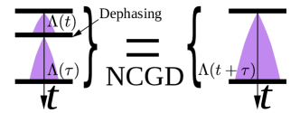
Figure 1: Illustrative sketch of the property of NCGD dynamics: fixed a reference basis, applying dephasing at an intermediate instant of the dynamics does not change the state transformation, if dephasing is also applied at the initial and final time.

Recently there has been considerable interest in incoherent operations aaberg2014catalytic ; Baumgratz2014 ; Streltsov2017 ; Liu2017 , which are defined for maps only. In contrast here we investigate dynamics. We can compare our notion with the literature by fixing $t=\tau$ in the Definition 3, thus referring it to one map, $\Lambda\equiv\Lambda(t)$, which we call CGD map. There are two interesting subsets of NCGD maps. One is the subset that does not create coherence from incoherent states, which is described by $\Delta\circ\Lambda\circ\Delta=\Lambda\circ\Delta$; this is the maximal set of incoherent operations aaberg2014catalytic . The other noteworthy subset of NCGD maps is the coherence nonactivating set fixed by $\Delta\circ\Lambda\circ\Delta=\Delta\circ\Lambda$; here, since the populations are independent of the initial coherence, the coherence is not a useable resource Liu2017 . Operations that are neither incoherent nor coherence nonactivating may still be NCGD, if the subspaces where coherence is generated are different from the ones detecting it (see App. D for a detailed example).

We conclude that NCGD dynamics can be understood by the propagated population not depending on the generated coherences. In addition, we can provide a direct operational meaning to (N)CGD, as ensured by the following proposition, which is proved in App: B.

Proposition 1. Given a non-degenerate reduced observable $\hat{X}=\sum_{x}x\ket{\psi_{x}}\!\bra{\psi_{x}}$ and the Lindblad dynamics $\left\{\Lambda(t)=e^{\mathcal{L}t}\right\}_{t\in\mathbbm{R^{+}}}$, the latter is NCGD if and only if the conditional probabilities $Q^{\hat{X}}_{1|1}\left\{x,t|x_{0},0\right\}$ satisfy $\forall t\geq s\in\mathbbm{R^{+}}$

$$Q^{\hat{X}}_{1|1}\left\{x,t|x_{0},0\right\}=\sum_{y}Q^{\hat{X}}_{1|1}(x,t-s|y,0)Q^{\hat{X}}_{1|1}(y,s|x_{0},0).$$ (6)

The condition in Eq.(6) is simply the (homogeneous) Chapman-Kolmogorov equation vanKampen1992 ; Breuer2002 ; Gardiner2004 , which is always satisfied by a classical Markov (homogeneous) process, but, indeed, not necessarily by a quantum one. As we will see, the relation between NCGD and classicality relies on Proposition 1. For the moment, let us stress that Eq.(6) can be in principle easily checked in practice, since the conditional probabilities $Q^{\hat{X}}_{1|1}\left\{x,t|x_{0},0\right\}$ can be reconstructed by preparing the system in one eigenstate of $\hat{X}$ and measuring $\hat{X}$ itself at a final time $t$, without the need to access intermediate steps of the evolution.

The previous proposition also allows us to connect CGD with other easily accessible quantities, which are already well-known in the literature. As a significant example, let us mention the LGtIs Huelga1995 ; Emary2014 , which were introduced to characterize macroscopic realistic theories, that is, classical theories where physical systems possess definite values (whether or not they are measured) and such values can be accessed without changing the state of the system. In particular, in LGtIs the Leggett-Garg non-invasiveness requirement Leggett1985 is replaced by an assumption which turns out to be related to Markovianity Emary2014 . Given a dichotomic observable $X$ with values in $\left\{0,1\right\}$ and the related correlation function, which in the quantum framework is defined as $C_{X}(t,0)=\sum_{x,x_{0}}Q^{\hat{X}}_{2}\left\{x,t;x_{0},0\right\}xx_{0}$, the LGtI we consider here reads $\left|2C_{X}(t,0)-C_{X}(2t,0)\right|\leq\langle X(0)\rangle$, with $\langle X(0)\rangle$ the expectation value of $X$ at the initial time. Now, since the validity of Eq.(6) is a sufficient condition for the LGtI to be satisfied, see App.B, Proposition 1 directly leads us to the following.

Theorem 1. Given a Lindblad dynamics, the LGtI is violated only if the dynamics is CGD.

The Theorem thus clarifies how the LGtI can be used to witness that coherences are generated by the dynamics and subsequently turned into populations.

Quantum coherence and non-classicality

We are now in the position to state the main result of our paper. In the previous section we have seen how the NGDC property of the dynamics is related with the Chapman-Kolmogorov composition law for the conditional probabilities with respect to the initial time [see Proposition 1]. However, if we want to establish a definite connection between coherences and (non-)classicality, we need to take a step further and to go beyond the one-time statistics to access the higher orders of the hierarchy of probabilities, since only the latter encompass the definite meaning of classicality we are referring to.

The recalled notion of quantum Markovianity for multi-time statistics does provide us with the wanted link among coherences and classicality. This is shown by the following Theorem, whose proof is presented in App.C.

Theorem 2. Given a non-degenerate reduced observable $\hat{X}=\sum_{x}x\ket{\psi_{x}}\!\bra{\psi_{x}}$ and a jM hierarchy of probabilities $Q^{\hat{X}}_{n}\left\{x_{n},t_{n};\ldots x_{1},t_{1}\right\}$, the latter is jCL for any initial diagonal state $\rho(0)=\sum_{x_{0}}p_{x_{0}}\ket{\psi_{x_{0}}}\!\bra{\psi_{x_{0}}}$ if and only if the dynamics $\left\{\Lambda(t)=e^{\mathcal{L}t}\right\}_{t\in\mathbbm{R}^{+}}$ is NCGD.

Theorem 2 means that if the multi-time statistics is Markovian, the capability of a dynamics to generate coherences and turn them into populations is in one-to-one correspondence with non-classicality. In other words, Markovianity guarantees the wanted connection between a property of the coherences, which is fixed by the dynamics, and the classicality of the multi-time probability distributions. This is a direct consequence of the peculiarity of Markovian processes, classical as well as quantum, which allows one to reconstruct the higher order probability distributions from the lowest order one.

Finally, the previous Theorem also allows us to clarify to what extent the LGtI is actually related with non-classicality, since it directly implies the following.

Theorem 3. Given a 2M hierarchy of probabilities, the LGtI is violated only if the hierarchy is non-classical.

For the sake of clarity, in Fig.2 we report a summary of the theorems presented in this paper, which establish definite connections among the notions of classicality, quantum coherence (in particular NCGD of the dynamics) and LGtI.

Figure 2: Implication structure of the main results of the paper. The notion of $j$-classicality is given in Definition 1, $j$-Markovianity in Definition 2 and the property of the evolution of coherence named NCGD, which stands for non-coherence-generating-and-detecting, in Definition 3; finally LGtI denotes the Leggett-Garg type inequality Huelga1995 considered here. A Lindblad dynamics is always assumed.

Non-Markovian multi-time statistics

In the last part of the paper, we start to explore the general case of non-Markovian multi-time statistics. Indeed, now the connection between quantum coherence and the non-classicality of the multi-time statistics is no longer guaranteed, since the higher order probabilities cannot be inferred from the lowest order ones. Exploiting a model which traces back to Lindblad himself Lindblad1980 ; Accardi1982 , we show that this connection is lost even in the presence of a simple Lindblad dynamics. Remarkably, there can be a genuinely non-classical statistics associated with the measurements of an observable without that any quantum coherence of such observable is ever present in the state of the measured system.

Consider a two-level system, $\mathcal{H}_{S}=\mathbbm{C}^{2}$, interacting with a continuous degree of freedom, $\mathcal{H}_{E}=\mathcal{L}(\mathbbm{R})$, via the unitary operators defined by $U(t)\ket{\ell,p}=e^{i\ell pt}\ket{\ell,p},$ where $\left\{\ket{\ell}\right\}_{\ell=-1,1}$ is the eigenbasis of the system operator $\hat{\sigma}_{z}$ and $\left\{\ket{p}\right\}_{p\in\mathbbm{R}}$ is an improper basis of $\mathcal{H}_{E}$. Assuming an initial product state and a pure environmental state, $\rho_{E}(0)=\ket{\varphi_{E}}\!\bra{\varphi_{E}}$ with $\ket{\varphi_{E}}=\int_{-\infty}^{\infty}dpf(p)\ket{p}$, the open-system dynamics is pure dephasing, fixed by $\rho_{-11}(t)=\rho_{-11}(0)k(t)$ with $k(t)=\int_{-\infty}^{\infty}dp|f(p)|^{2}e^{2ipt}$, where $\rho_{-11}=\bra{-1}\rho\ket{1}$. We consider projective measurements of $\hat{\sigma}_{x}$, whose eigenbasis is denoted as $\left\{\ket{+},\ket{-}\right\}$, and then we assume initial states as $\rho(0)=p_{+}\ket{+}\!\bra{+}+p_{-}\ket{-}\!\bra{-}$. In App.E we report the exact two-time probability $Q^{\hat{\sigma}_{x}}_{2}$, given by Eq.(1), and the probability $Q^{\hat{\sigma}_{x}}_{2M}$ one would get for a Markovian statistics, see Eq.(4), along with the conditions for the dynamics to be CGD and the statistics 2CL.

First, consider an initial Lorentzian distribution, $|f(p)|^{2}=\Gamma\pi^{-1}/(\Gamma^{2}+(p-p_{0})^{2}),$ so that the decoherence function is given exactly by an exponential, $k(t)=e^{2ip_{0}t}e^{-2\Gamma t},$ and the open-system dynamics is fixed by the pure dephasing Lindblad equation Guarnieri2014 . Nevertheless, the QRT in Eq.(4) is generally not satisfied, not even by the two-time probability distributions, so that the multi-time statistics is NM. The difference, also qualitative, among the exact joint probability distribution $Q^{\hat{\sigma}_{x}}_{2}$ and the Markovian one $Q^{\hat{\sigma}_{x}}_{2M}$ is illustrated in Fig.3 a). Furthermore, one can easily see App.E that the Kolmogorov condition for $n=2$ does not hold, $\sum_{y}Q^{\hat{\sigma}_{x}}_{2}\left\{+,t;y,s\right\}\neq Q^{\hat{\sigma}_{x}}_{1}\left\{+,t\right\}$. The statistics at hand is hence non-classical. On the other hand, the corresponding Lindblad dynamics (for $p_{0}=0$) is NCGD: pure dephasing on $\hat{\sigma}_{z}$ cannot even generate coherences of $\hat{\sigma}_{x}$ (of course, this also implies that the corresponding LGtI is always satisfied). We conclude that, despite the non-classicality of the statistics, the coherences of the measured observable $\hat{\sigma}_{x}$ are not involved at all in the dynamics: at no point in time the state of the measured system has non-zero coherence with respect to $\hat{\sigma}_{x}$.

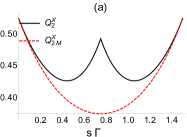
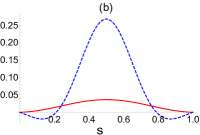
Figure 3: a) Exact two-time probability $Q^{\hat{\sigma}_{x}}_{2}\left\{+,t;+,s\right\}$ [see Eq.(1)] (solid black line) and 2M probability $Q^{\hat{\sigma}_{x}}_{2M}\left\{+,t;+,s\right\}$ [see Eq.(4)] (dashed red line) as functions of $s$, for a Lorentzian $|f(p)|^{2}$. The parameters are $t=1.5\Gamma^{-1},p_{0}=0$. b) Amount of CGD (according to the general definition given in App.E) quantified via the infinity norm, (solid, red line) and violation of the Kolmogorov condition [i.e., $|\sum_{y}Q^{\hat{\sigma}_{x}}_{2}\left\{+,t;y,s\right\}-Q^{\hat{\sigma}_{x}}_{1}\left\{+,t\right\}|$] (dashed, blue line) as functions of $s$, for $|f(p)|^{2}$ given by the superposition of two Gaussians. The parameters are $A_{1}=A_{2}=1/(2\sqrt{2\pi}),\sigma_{1}=\sigma_{2}=\sigma,\sigma=p_{1}=t=1,p_{2}=2p_{1}$.

In a complementary way, we exemplify how the instants where the multi-time statistics satisfies the Kolmogorov conditions may coincide with instants where coherences are generated and converted into populations. However, we have to leave open the question of whether there is a fully classical statistics (for any sequence of times), while the dynamics of the coherences is non-trivial. Take an initial distribution given by the sum of two Gaussians, $|f(p)|^{2}=\sum_{i=1,2}A_{i}\exp\left(-(p-p_{i})^{2}/(2\sigma^{2}_{i})\right)$. Once again one can easily see that the statistics is NM [see App.E], but this time the dynamics is generally CGD. Nevertheless, the creation and detection of coherences is not in correspondence with the non-classicality of the statistics. In Fig.3 b), we can see that there are instants of time where the dynamics is CGD, but the statistics is 2CL, see also App.E; note that at these same instants of time also the Chapman-Kolmogorov condition in Eq.(6) does not hold. By investigation (not reported here) of the model at hand in a wide region of parameters, we also observe that there does not seem to be a threshold in the amount of CGD, above which the violation of 2CL is guaranteed.

The previous examples illustrate the essential role of Markovianity to establish a precise link between quantum coherence, or any other dynamical property, and non-classicality. In addition, they imply that the coherences themselves cannot be used as a witness of non classicality, without any a-priori information about higher order probabilities. To know whether coherences are linked to jCL, one needs to access $Q^{\hat{X}}_{j}$ to verify jM, but then jCL can be directly checked via the Kolmogorov conditions.

Conclusions

We proved a one-to-one correspondence between the non-classicality of the multi-time statistics associated with sequential measurements of one observable at different times and the quantum coherence with respect to the eigenbasis of the measured observable itself. We pointed out the key property of quantum coherence which is directly linked with non classicality, connecting it to the recently developed resource theory of coherence. Furthermore, we illustrated the essential role of Markovianity in linking dynamical properties, such as the evolution of quantum coherence or the violation of the LGtI, to higher order probability distributions of the multi-time statistics and hence to (non-) classicality.

Our approach will naturally apply to several areas where the possible quantum origin of certain physical phenomena is under debate, such as quantum biology or quantum thermodynamics. We plan to exploit the results presented here to study some relevant examples taken from these fields of research. In addition, we want to extend our analysis to classical theories with invasive measurements starting from the notion of signaling in time; in particular, we think that our approach will further motivate the investigation of the scenario in which memory effects are present, at the level of the quantum multi-time statistics and/or of the measurement invasiveness Montina2012 ; Frustaglia2016 ; Cabello2018 . Finally, it will be of interest to include the description of non projective measurements, as well as the measurement of multiple, non-commuting observables.

Acknowledgments We acknowledge very interesting and fruitful discussions with Thomas Theurer and Benjamin Desef, as well as financial support by the ERC Synergy Grant BioQ (grant no 319130), the EU project QUCHIP (grant no. 641039) and Fundación ”la Caixa”.

Appendix A Quantum regression theorem and quantum Markovianity

Here we want to discuss more in detail why the QRT can be naturally seen as the quantum counterpart of the Markov condition for the hierarchy of probabilities defined in the main text.

Now, let

$$Q^{\hat{X}}_{k|n}\left\{x_{n+k},t_{n+k};\ldots x_{n+1},t_{n+1}|x_{n},t_{n};\ldots x_{1},t_{1}\right\}=\frac{Q^{\hat{X}}_{k+n}\left\{x_{n+k},t_{n+k};\ldots x_{1},t_{1}\right\}}{Q^{\hat{X}}_{n}\left\{x_{n},t_{n};\ldots x_{1},t_{1}\right\}}$$ (7)

be the conditional probability distributions associated with the hierarchy of probability distributions defined in Eq.(1) of the main text, referred to a reduced observable $\hat{X}\otimes\mathbbm{1}$ (we keep implying the subfix $S$ for the sake of simplicity); Eq.(7) can be easily obtained from the general definition based on the conditional state Gardiner2004 , using the projectors into the eigenspaces of $\hat{X}\otimes\mathbbm{1}$, which are degenerate with respect to the global space $\mathcal{H}$. If we now express the right hand side of the previous relation via the QRT, i.e., Eq.(4) of the main text, we can exploit the non-degeneracy of $\hat{X}$ on $\mathcal{H}_{S}$. Because of that, for any couple of reduced super-operators $\mathcal{A}$ and $\mathcal{B}$ we have

$$\frac{\mbox{tr}_{S}\left\{\mathcal{A}\mathcal{P}_{x}\rho_{S}\right\}}{\mbox{tr}_{S}\left\{\mathcal{B}\mathcal{P}_{x}\rho_{S}\right\}}=\frac{\mbox{tr}_{S}\left\{\mathcal{A}[\ket{\psi_{x}}\!\bra{\psi_{x}}]\right\}}{\mbox{tr}_{S}\left\{\mathcal{B}[\ket{\psi_{x}}\!\bra{\psi_{x}}]\right\}},$$

from which one can easily see that the hierarchy defined in Eq.(4) of the main text satisfies the condition

$$Q^{\hat{X}_{S}}_{1|n}\left\{x_{n+1},t_{n+1}|x_{n},t_{n};\ldots x_{1},t_{1}\right\}=Q^{\hat{X}_{S}}_{1|1}\left\{x_{n+1},t_{n+1}|x_{n},t_{n}\right\}$$

$$=\mbox{tr}_{S}\left\{\mathcal{P}_{x_{n+1}}e^{\mathcal{L}(t_{n+1}-t_{n})}[\ket{\psi_{x_{n}}}\!\bra{\psi_{x_{n}}}]\right\}.$$ (8)

The first equality in the previous equation is the Markov condition, which defines Markov stochastic processes Breuer2002 ; Gardiner2004 . Actually, the QRT is at the basis of the definition of quantum Markov processes put forward by Lindblad in Lindblad1979 (see also the more recent definitions in Fleming2011 ; LoGullo2014 ).

On the other hand, different approaches have been followed to introduce a definition of quantum Markovianity which can be referred to the dynamics of the open quantum systems tout-court. Indeed, the hierarchy of probabilities in Eq.(1), or in Eq.(4), of the main text depends on the specific measurement procedure one is taking into account. Moreover and more importantly, the measurements at intermediate times involved in that definition modify the correlations between the system and the environment, thus modifying the subsequent dynamics of the open system Breuer2016 . Hence, in order to assign the Markovian or non-Markovian attribute to the open system dynamics solely, different definitions have been put forward (see the recent reviews Rivas2014 ; Breuer2016 ), relying directly on properties of the dynamical maps $\left\{\Lambda(t)\right\}_{t\in\mathbbm{R}^{+}}$. Of course, the Markovianity referring to the dynamics solely and that referring to the multi-time probability distributions are quite different concepts, since in general the one-time statistics (and the related dynamical maps) does not allow to infer the behavior of higher order distributions Vacchini2011 , and then, e.g., whether the QRT holds or not. The ‘proper’ definition of quantum Markovianity ultimately depends on the framework one is interested in. Here, as said in Definition 2, we identify quantum Markov processes with those satisfying the QRT.

Finally, let us note that the Markov condition in Eq.(8) implies that, also in the quantum case, the whole hierarchy of probabilities is fixed by the initial condition and the $Q^{\hat{X}_{S}}_{1|1}$ conditional probabilities, i.e., we have for any $x_{1},\ldots x_{n},t_{n}\geq\ldots\geq t_{1}$

$$Q^{\hat{X}_{S}}_{n}\left\{x_{n},t_{n};\ldots;x_{2},t_{2};x_{1},t_{1}\right\} =\left(\prod_{k=1}^{n-1}Q^{\hat{X}_{S}}_{1|1}\left\{x_{k+1},t_{k+1}|x_{k},t_{k}\right\}\right)Q^{\hat{X}_{S}}_{1}\left\{x_{1},t_{1}\right\}$$

$$=\left(\prod_{k=1}^{n-1}\mbox{tr}\left\{\mathcal{P}_{x_{k+1}}e^{\mathcal{L}(t_{k+1}-t_{k})}\left[\ket{\psi_{x_{k}}}\!\bra{\psi_{x_{k}}}\right]\right\}\right)\mbox{tr}\left\{\mathcal{P}_{x_{1}}e^{\mathcal{L}t_{1}}\rho_{S}(0)\right\},$$

where in the second line we used that since we are focusing on the Lindblad dynamics we have

$$Q^{\hat{X}_{S}}_{1|1}\left\{x,t|y,s\right\}=\mbox{tr}_{S}\left\{\mathcal{P}_{x}e^{\mathcal{L}(t-s)}\left[\ket{\psi_{y}}\!\bra{\psi_{y}}\right]\right\}=Q^{\hat{X}_{S}}_{1|1}\left\{x,t-s|y,0\right\}.$$ (10)

Appendix B Proof of the Proposition 1 and Theorem 1.

Before proving the Proposition 1, we need to prove the following Lemma.

Lemma 1.

The evolution fixed by the Lindblad dynamics $\left\{\Lambda(t)=e^{\mathcal{L}t}\right\}_{t\in\mathbbm{R}^{+}}$ is NCGD if and only if

$$\sum_{y\neq z}\bra{\psi_{\tilde{x}}}\Lambda(t)[\ket{\psi_{y}}\!\bra{\psi_{z}}]\ket{\psi_{\tilde{x}}}\bra{\psi_{y}}\Lambda(\tau)\left[\ket{\psi_{x}}\!\bra{\psi_{x}}\right]\ket{\psi_{z}}=0\quad\forall x,\tilde{x};t,\tau\in\mathbbm{R}^{+}.$$ (11)

Proof.

First note that $\left\{\Lambda(t)\right\}_{t\in\mathbbm{R}^{+}}$ satisfies Eq.(11) if and only if $\forall x,\tilde{x};t,s\in\mathbbm{R}^{+}$

$$\bra{\psi_{\tilde{x}}}\;\Lambda(t)\circ\Lambda(\tau)\left[\ket{\psi_{x}}\!\bra{\psi_{x}}\right]\;\ket{\psi_{\tilde{x}}}$$

$$=\sum_{y,z}\bra{\psi_{\tilde{x}}}\;\Lambda(t)\Big{[}\ket{\psi_{y}}\!\bra{\psi_{y}}\;\Lambda(\tau)\left[\ket{\psi_{x}}\!\bra{\psi_{x}}\right]\;\ket{\psi_{z}}\!\bra{\psi_{z}}\Big{]}\;\ket{\psi_{\tilde{x}}}$$

$$=\sum_{y}\bra{\psi_{\tilde{x}}}\;\Lambda(t)\Big{[}\ket{\psi_{y}}\!\bra{\psi_{y}}\;\Lambda(\tau)\left[\ket{\psi_{x}}\!\bra{\psi_{x}}\right]\;\ket{\psi_{y}}\!\bra{\psi_{y}}\Big{]}\;\ket{\psi_{\tilde{x}}}$$

$$=\bra{\psi_{\tilde{x}}}\;\Lambda(t)\circ\Delta\circ\Lambda(\tau)\left[\ket{\psi_{x}}\!\bra{\psi_{x}}\right]\;\ket{\psi_{\tilde{x}}},$$ (12)

since the first and the last equalities are always valid, while the second is Eq.(11), adding the diagonal terms on both sides. We first prove that if $\left\{\Lambda(t)\right\}_{t\in\mathbbm{R}^{+}}$ is NCGD then the above equality holds. We can in fact rewrite the first line as

$$\sum_{k,k^{\prime}}\bra{\psi_{\tilde{x}}}\ket{\psi_{k}}\!\bra{\psi_{k}}\;\Lambda(t)\circ\Lambda(\tau)\big{[}\ket{\psi_{k^{\prime}}}\!\bra{\psi_{k^{\prime}}}\ket{\psi_{x}}\!\bra{\psi_{x}}\ket{\psi_{k^{\prime}}}\!\bra{\psi_{k^{\prime}}}\big{]}\;\ket{\psi_{k}}\!\bra{\psi_{k}}\ket{\psi_{\tilde{x}}}$$

$$=\bra{\psi_{\tilde{x}}}\;\Delta\circ\Lambda(t)\circ\Lambda(\tau)\circ\Delta\left[\ket{\psi_{x}}\!\bra{\psi_{x}}\right]\;\ket{\psi_{\tilde{x}}}$$ (13)

$$=\bra{\psi_{\tilde{x}}}\;\Delta\circ\Lambda(t)\circ\Delta\circ\Lambda(\tau)\circ\Delta\left[\ket{\psi_{x}}\!\bra{\psi_{x}}\right]\;\ket{\psi_{\tilde{x}}}$$

$$=\bra{\psi_{\tilde{x}}}\;\Lambda(t)\circ\Delta\circ\Lambda(\tau)\left[\ket{\psi_{x}}\!\bra{\psi_{x}}\right]\;\ket{\psi_{\tilde{x}}}.$$

where in the first line we used that only the terms $\tilde{x}=k$,$x=k^{\prime}$ are non-zero, and in the third line we used that $\left\{\Lambda(t)\right\}_{t\in\mathbbm{R}^{+}}$ is NCGD.

For the converse, we start with the assumption that the equality (12) holds for any $x,\tilde{x},t,\tau\in\mathbbm{R}^{+}$. The statement then simply follows by the linearity of the propagators since $\Delta$ is a projection onto the span of $\{\ket{\psi_{x}}\!\bra{\psi_{x}}\}_{x}$. ∎

We can now prove the Proposition 1.

Proof.

Using Eq.(3) of the main text and Eq.(10) we have that

$$Q^{\hat{X}}_{1|1}\left\{x,t|x_{0},0\right\}-\sum_{y}Q^{\hat{X}}_{1|1}(x,t-s|y,0)Q^{\hat{X}}_{1|1}(y,s|x_{0},0)$$

$$=\bra{\psi_{x}}\Lambda(t)\left[\ket{\psi_{x_{0}}}\!\bra{\psi_{x_{0}}}\right]\ket{\psi_{x}}-\sum_{y}\bra{\psi_{x}}\Lambda(t-s)\left[\ket{\psi_{y}}\!\bra{\psi_{y}}\right]\ket{\psi_{x}}*\bra{\psi_{y}}\Lambda(s)\left[\ket{\psi_{x_{0}}}\!\bra{\psi_{x_{0}}}\right]\ket{\psi_{y}},$$

so that using the semigroup composition law $\Lambda(t)=\Lambda(t-s)\Lambda(s)$ and the resolution of the identity, the first term in the previous expression can be written as

$$\bra{\psi_{x}}\Lambda(t-s)\big{[}\Lambda(s)\left[\ket{\psi_{x_{0}}}\!\bra{\psi_{x_{0}}}\right]\big{]}\ket{\psi_{x}}$$

$$=\sum_{y,y^{\prime}}\bra{\psi_{x}}\Lambda(t-s)\Big{[}\ket{\psi_{y}}\!\bra{\psi_{y}}\Lambda(s)\left[\ket{\psi_{x_{0}}}\!\bra{\psi_{x_{0}}}\right]\ket{\psi_{y^{\prime}}}\!\bra{\psi_{y^{\prime}}}\Big{]}\ket{\psi_{x}},$$

$$=\sum_{y,y^{\prime}}\bra{\psi_{x}}\Lambda(t-s)\left[\ket{\psi_{y}}\bra{\psi_{y^{\prime}}}\right]\ket{\psi_{x}}\bra{\psi_{y}}\Lambda(s)\left[\ket{\psi_{x_{0}}}\!\bra{\psi_{x_{0}}}\right]\ket{\psi_{y^{\prime}}},$$

so that the ‘diagonal terms’ (with $y=y^{\prime}$) cancel out with the second contribution and the violation of the homogeneous Chapman-Kolmogorov condition is given by

$$Q^{\hat{X}}_{1|1}\left\{x,t|x_{0},0\right\}-\sum_{y}Q^{\hat{X}}_{1|1}(x,t-s|y,0)Q^{\hat{X}}_{1|1}(y,s|x_{0},0)$$

$$=\sum_{y\neq y^{\prime}}\bra{\psi_{x}}\Lambda(t-s)\left[\ket{\psi_{y}}\bra{\psi_{y^{\prime}}}\right]\ket{\psi_{x}}\bra{\psi_{y}}\Lambda(s)\left[\ket{\psi_{x_{0}}}\!\bra{\psi_{x_{0}}}\right]\ket{\psi_{y^{\prime}}},$$ (14)

which implies that such difference is equal to 0 for any $x_{0},x,t\geq s$ if and only if the Lindblad dynamics is NCGD, see Eq.(11). ∎

Now, Theorem 1 easily follows from the following Lemma.

Lemma 2.

Consider a dichotomic observable $\hat{X}$ with values in $\left\{0,1\right\}$ and such that the conditional probabilities $Q^{\hat{X}}_{1|1}\left\{x,t;x_{0},0\right\}$ satisfy Eq.(6) of the main text, then the correlation function $C_{X}(t,0)$ satisfies the LGtI

$$\left|2C_{X}(t,0)-C_{X}(2t,0)\right|\leq\langle X(0)\rangle.$$ (15)

Proof.

First note that

$$C_{X}(t,0):=\sum_{x,x_{0}=0,1}Q^{\hat{X}}_{2}\left\{x,t;x_{0},0\right\}x*x_{0}=Q^{\hat{X}}_{2}\left\{1,t;1,0\right\};$$

since the dichotomic observable has values in $\left\{0,1\right\}$; thus

$$\left|2C_{X}(t,0)-C_{X}(2t,0)\right|=\left|2Q^{\hat{X}}_{2}\left\{1,t;1,0\right\}-Q^{\hat{X}}_{2}\left\{1,2t;1,0\right\}\right|$$

$$=\left|2Q^{\hat{X}}_{1|1}\left\{1,t|1,0\right\}-Q^{\hat{X}}_{1|1}\left\{1,2t|1,0\right\}\right|Q^{\hat{X}}_{1}\left\{1,0\right\}$$

$$=\left|2Q^{\hat{X}}_{1|1}\left\{1,t|1,0\right\}-\sum_{x_{k}k=0,1}Q^{\hat{X}}_{1|1}\left\{1,t|x_{k},0\right\}Q^{\hat{X}}_{1|1}\left\{x_{k},t|1,0\right\}\right|Q^{\hat{X}}_{1}\left\{1,0\right\},$$ (16)

which provides us with Eq.(15), since $\langle X(0)\rangle=Q^{\hat{X}}_{1}\left\{1,0\right\}$, while $2Q^{\hat{X}}_{1|1}\left\{1,t|1,0\right\}-\sum_{x_{k}k=0,1}Q^{\hat{X}}_{1|1}\left\{1,t|x_{k},0\right\}Q^{\hat{X}}_{1|1}\left\{x_{k},t|1,0\right\}$ is maximized by 1 for $Q^{\hat{X}}_{1|1}\left\{1,t|1,0\right\}=1$ or $Q^{\hat{X}}_{1|1}\left\{1,t|1,0\right\}=0$ and $Q^{\hat{X}}_{1|1}\left\{0,t|1,0\right\}=1$ (as seen using $Q^{\hat{X}}_{1|1}\left\{1,t|0,0\right\}=1-Q^{\hat{X}}_{1|1}\left\{1,t|1,0\right\}$). ∎

Note that Lemma 2 holds independently of whether the conditional probabilities are referring to the quantum setting (and hence are defined as in Eq.(1) of the main text) or are directly referring to a classical theory: our proof goes along the same line as that in Lambert2010 , simply adapting it to (possibly) quantum conditional probabilities.

Appendix C Proof of Theorem 2 and Theorem 3.

Before presenting the proof to Theorem 2, let us give the basic idea behind it. The time-homogeneous Chapman-Kolmogorov equation holds for any classical time-homogeneous Markov process, that is, Markovianity and classicality imply Chapman-Kolmogorov; note that the time-homogeneity of the statistics holds, as a consequence of (2)M and the Lindblad dynamics [see Eq.(10)]. For the converse, we can exploit the definition of jM, which provides us with a notion of Markovianity beyond classical processes, i.e., for any quantum statistics. As said, the Markov property (both for classical and nonclassical statistics) connects the multi-time probability distributions to the initial one-time distribution and the conditional probability $Q^{\hat{X}}_{1|1}$; as a direct consequence of this, it is then easy to see that, if the Chapman-Komogorov equation holds, jM directly turns into jCL. Theorem 2 thus follows from the equivalence established in Proposition 1.

Explicitly, both the Theorems 2 and 3 directly follow from the following Lemma.

Lemma 3.

Given a non-degenerate observable $\hat{X}=\sum_{x}x\ket{\psi_{x}}\!\bra{\psi_{x}}$ and a jM hierarchy of probabilities, the latter defines a jCL statistics for any initial diagonal state $\rho(0)=\sum_{x_{0}}p_{x_{0}}\ket{\psi_{x_{0}}}\!\bra{\psi_{x_{0}}}$ if and only if Eq.(6) of the main text holds for the quantum conditional probability $Q^{\hat{X}}_{1|1}\left\{x,t|x_{0},0\right\}$.

Proof.

“Only if”: the statistics is, in particular, 2CL, so that we have, for any $x,t\geq s\in\mathbbm{R}^{+}$,

$$\sum_{y}Q^{\hat{X}}_{2}\left\{x,t;y,s\right\}=Q^{\hat{X}}_{1}\left\{x,t\right\}.$$

But then, using the definition of conditional probability $Q^{\hat{X}}_{2}\left\{x,t;y,s\right\}=Q^{\hat{X}}_{1|1}\left\{x,t|y,s\right\}*Q^{\hat{X}}_{1}\left\{y,s\right\}$ and, crucially, the time-homogeneity guaranteed by the 2M and the Lindblad equation (see Eq.(10)), we can write

$$\sum_{y}Q^{\hat{X}}_{1|1}\left\{x,t-s|y,0\right\}*Q^{\hat{X}}_{1}\left\{y,s\right\}=Q^{\hat{X}}_{1}\left\{x,t\right\}.$$

Using the Kolmogorov condition, this time w.r.t. the initial value, and the definition of conditional probability, the previous relation gives

$$\sum_{x_{0}}Q^{\hat{X}}_{1}\left\{x_{0},0\right\}\left(\sum_{y}Q^{\hat{X}}_{1|1}\left\{x,t-s|y,0\right\}*Q^{\hat{X}}_{1|1}\left\{y,s|x_{0},0\right\}-Q^{\hat{X}}_{1|1}\left\{x,t|x_{0},0\right\}\right)=0,$$

which directly provides us with the Chapman-Kolmogorov composition law in Eq.(6) of the main text, since, by assumption, we can choose any initial diagonal state $\rho(0)=\sum_{x_{0}}p_{x_{0}}\ket{\psi_{x_{0}}}\!\bra{\psi_{x_{0}}}$, and then any distribution of $Q^{\hat{X}}_{1}\left\{x_{0},0\right\}=p_{x_{0}}$.

“If”: Eq.(6) of the main text for the quantum conditional probability $Q^{\hat{X}}_{1|1}\left\{x,t|x_{0},0\right\}$ means that

$$\mbox{tr}\left\{\mathcal{P}_{x}e^{\mathcal{L}t}\left[\ket{\psi_{x_{0}}}\!\bra{\psi_{x_{0}}}\right]\right\}=\sum_{x_{k}}\mbox{tr}\left\{\mathcal{P}_{x}e^{\mathcal{L}(t-s)}\left[\ket{\psi_{x_{k}}}\!\bra{\psi_{x_{k}}}\right]\right\}\mbox{tr}\left\{\mathcal{P}_{x_{k}}e^{\mathcal{L}s}\left[\ket{\psi_{x_{0}}}\!\bra{\psi_{x_{0}}}\right]\right\}$$

$$\forall x_{0},x;t\geq s\in\mathbbm{R}^{+},$$

which, replaced in Eq.(A), implies Eq.(2) of the main text [$s\mapsto t_{k}-t_{k-1},x_{0}\mapsto x_{k-1},t\mapsto t_{k+1}-t_{k-1},x\mapsto x_{k+1}$], so that if the hierarchy is jM it will also be jCL; note that this is the case also for $k=1$ since we assume the initial state to be diagonal in the selected basis. ∎

Theorem 2 hence directly follows from Lemma 3 and Proposition 1, while Theorem 3 follows, e.g., from Lemmas 2 and 3.

Appendix D Difference between the various types of incoherent operations

Let us start by presenting a very simple example of an evolution which is CGD, i.e., which can generate and detect coherence [see Eq.(5) of the main text] and which, in addition, allows us to connect such property with nonclassicality in an easy way. Hence, consider a two-level system, initially in the eigenstate $\ket{-1}$ of $\hat{\sigma}_{z}$ (where $\left\{\ket{\ell}\right\}_{\ell=-1,1}$ is the eigenbasis of the operator $\hat{\sigma}_{z}$) and evolving under the unitary operators

$$U(t)=e^{-i\hat{\sigma}_{y}t}.$$ (17)

Indeed, this evolution can generate coherence with respect to $\hat{\sigma}_{z}$ at an intermediate time, i.e., there are times $t_{1}>0$ when $|\bra{\pm 1}U(t_{1})\ket{-1}\bra{-1}U^{{\dagger}}(t_{1})\ket{\mp 1}|\neq 0$, and can convert such coherence into populations, i.e. there are times $t_{2}$ such that $\bra{1}U(t_{2}-t_{1})\ket{\mp 1}\bra{\pm 1}U^{{\dagger}}(t_{2}-t_{1})\ket{1}\neq 0$, which implies that the condition in Eq.(5) of the main text is satisfied: the evolution is CGD; see also Fig.4 a). An important point of this example is that, since the evolution is unitary, the QRT is automatically guaranteed [i.e, Eq.(1) and Eq.(4) of the main text coincide], so that the two-time statistics associated with measurements of the observable $\hat{\sigma}_{z}$ is simply given by

$$Q_{2}^{\hat{\sigma}_{z}}\left\{1,t_{2};x,t_{1}\right\}=\left|\bra{1}U(t_{2}-t_{1})\ket{x}\right|^{2}\left|\bra{x}U(t_{1})\ket{-1}\right|^{2},$$

with $x=-1,1$. It is then easy to see that the CGD condition implies $\sum_{x}Q_{2}^{\hat{\sigma}_{z}}\left\{1,t_{2};x,t_{1}\right\}\neq Q_{1}^{\hat{\sigma}_{z}}\left\{1,t_{2}\right\}=\left|\bra{1}U(t_{2})\ket{-1}\right|^{2}$, so that the multitime statistics is nonclassical (see Definition 1 in the main text): the coherence generated at intermediate time $t_{1}$ and turned into population at time $t_{2}$ directly implies a violation of the Kolmogorov condition, i.e., nonclassicality. This is not surprising, since, by virtue of the Theorem 2, we know that nonclassicality and CGD of the system’s (nondegenerate) observables coincide, whenever the QRT holds. If this is not the case, the correspondence between nonclassicality and CGD is no longer guaranteed, as we will exemplify in the next Section.

As mentioned in the main text, it is trivial to see that the maximally incoherent operations (MIO) aaberg2014catalytic and the coherence nonactivating maps Liu2017 are subsets of the NCGD maps. What we show here is that they are strict subsets, by giving an explicit example. Consider the completely positive and trace preserving map acting on a basis of linear operators on $\mathbbm{C}^{2}$ as

$$\Lambda:\begin{array}[]{cc}\left(\begin{array}[]{cc}1&0\\ 0&0\\ \end{array}\right)&\left(\begin{array}[]{cc}0&1\\ 0&0\\ \end{array}\right)\\ \left(\begin{array}[]{cc}0&0\\ 1&0\\ \end{array}\right)&\left(\begin{array}[]{cc}0&0\\ 0&1\\ \end{array}\right)\\ \end{array}\mapsto\begin{array}[]{cc}\left(\begin{array}[]{cc}0.996&-0.003i\\ 0.003i&0.004\\ \end{array}\right)&\left(\begin{array}[]{cc}0.003&0.99\\ 0&-0.003\\ \end{array}\right)\\ \left(\begin{array}[]{cc}0.003&0\\ 0.99&-0.003\\ \end{array}\right)&\left(\begin{array}[]{cc}0.004&0.003i\\ -0.003i&0.996\\ \end{array}\right)\\ \end{array}.$$ (18)

The map is NCGD, while it both creates coherence and also is able to detect it. Explicitly:

$$\left\|\Delta\circ\Lambda\circ\Lambda\circ\Delta-\Delta\circ\Lambda\circ\Delta\circ\Lambda\circ\Delta\right\|_{\infty}=0,$$ (19)

$$\left\|\Lambda\circ\Delta-\Delta\circ\Lambda\circ\Delta\right\|_{\infty}=0.003,$$ (20)

$$\left\|\Delta\circ\Lambda-\Delta\circ\Lambda\circ\Delta\right\|_{\infty}=0.003,$$ (21)

where $\|\Lambda\|_{\infty}$denotes the infinity norm of the $4\times 4$ matrix given by the action of $\Lambda$ on the basis of operators on $\mathbbm{C}^{2}$; recall that the infinity norm is the maximum among the absolute sums of the columns. Indeed, the same is true for applying the map multiple times: the NCGD condition remains fulfilled, while the above norm increases to over 0.12, as shown in Fig. 4 c).

(a)                                                   (b)                                                   (c)
               

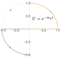
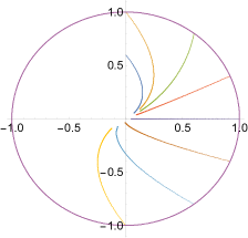
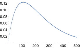
Figure 4: a) Example of an evolution fixed by Eq.(17) and by a possible measurement of $\hat{\sigma}_{z}$ at the intermediate time $t_{1}=\pi/4$: starting from $\ket{-1}$, the system’s state follows the solid blue line until $t_{1}$. If no measurement is performed, the system will then follow the dotted blue line, completely turning the coherence with respect to $\hat{\sigma}_{z}$ generated at $t_{1}$ into the population $\ket{1}$ at $t_{2}=\pi/2$. On the other hand, if a measurement at $t_{1}$ is performed, the state will be projected to $\ket{1}$ or $\ket{-1}$, with probability $1/2$ each; after that, the state will continue its evolution along the solid orange or blue line, respectively, so that a second measurement at time $t_{2}=\pi/2$ would still project the system’s state to $\ket{1}$ or $\ket{-1}$, with equal probabilities $1/2$. But then, we clearly have $1/2=\sum_{x=\pm 1}Q_{2}^{\hat{\sigma}_{z}}\left\{1,\pi/2;x,\pi/4\right\}\neq Q_{1}^{\hat{\sigma}_{z}}\left\{1,\pi/2\right\}=1$, i.e., the multitime statistics is nonclassical. b) Evolution of seven states on the XZ plane of the Bloch sphere under 1 to 300 applications of a map (see Eq. (18)) that is NCGD, but neither coherent nor coherence nonactivating. c) Norm of the difference between the coherent map in Eq. (18) and the incoherent one (see Eq. (20)) as a function of the number of applications. In this example this is the same as the norm of the difference between the coherence nonactivating and the actual evolution (see Eq. (21)).

Appendix E More details on the examples of NM multi-time statistics

In this Section, we provide the explicit calculations for the examples discussed in the main text. Let us emphasize that the model taken into account is very similar to the photonic system considered in Liu2013 to realize experimentally the transition between a Markovian and a non-Markovian dynamics, and further exploited in Guarnieri2014 to investigate the link between the dynamical notions of Markovianity and the QRT for system’s observables (rather than for the projective maps resulting from ideal selective measurements, as done here). There, the open system is given by the polarization degree of freedom of a photon, while the continuous degree of freedom represents the frequency of the photon, $\omega\in\mathbbm{R}^{+}$. Here, instead, we are taking into account a continuous degree of freedom, say the particle’s momentum, which can take on negative values, $p\in\mathbbm{R}$, for a reason which will become clear in a moment. Furthermore, essentially the same model (with coupling to position) has been studied in the context of dynamical decoupling in Arenz2015 .

Before proceeding, let us introduce more general definitions, which can be applied also to the non-Lindblad dynamics encountered in the following examples (in particular, in the second one, referring to an initial momentum distribution given by the superposition of two Gaussians). To do so, we need the notion of propagators of the dynamics, that is, the maps $\Lambda(t,s)$ (not necessarily completely positive, neither positive) such that

$$\Lambda(t)=\Lambda(t,s)\Lambda(s),$$ (22)

for any $t\geq s\in\mathbbm{R}^{+}$, so that $\rho(t)=\Lambda(t,s)[\rho(s)]$. For the sake of simplicity, we assume that the dynamics is divisible Breuer2016 , i.e., that the propagators can be defined as in Eq.(22) for any $t\geq s\in\mathbbm{R}^{+}$; indeed, this is always the case for a Lindbladian dynamics, where the propagators are defined by $\Lambda(t,s)=\Lambda(t-s,0)=e^{\mathcal{L}(t-s)}$.

We say that the multi-time statistics is j-Markovian if it satisfies the QRT theorem with respect to the dynamical maps and the corresponding propagators, i.e., if

$$Q^{\hat{X}_{S}}_{n}\left\{x_{n},t_{n}\ldots x_{1},t_{1}\right\}=\mbox{tr}_{S}\left\{\mathcal{P}_{x_{n}}\Lambda(t_{n},t_{n-1})\ldots\mathcal{P}_{x_{1}}\Lambda(t_{1})\rho_{S}(0)\right\},$$ (23)

for any $n\leq j,x_{1},\ldots x_{n},t_{n}\geq\ldots t_{1}$. Of course, this definition reduces to that in Eq.(4) of the main text if we consider a Lindblad dynamics. The validity of the QRT and a Lindblad dynamics ensure that the statistics is time-homogeneous, i.e., that the two-time conditional probabilities satisfy $Q^{\hat{X}}_{1|1}\left\{x,t|y,s\right\}=Q^{\hat{X}}_{1|1}\left\{x,t-s|y,0\right\}$. Hence, we can see the definition in Eq.(23) as the general definition of Markovian, possibly time-inhomogeneous statistics, while the definition in Eq.(4) of the main text corresponds to the Markovian time-homogeneous case.

Finally, we say that a (divisible) dynamics $\left\{\Lambda(t)\right\}_{t\in\mathbbm{R}^{+}}$, with propagators $\Lambda(t,s)$ is CGD whenever there exist instants $t\geq s\geq r\in\mathbbm{R}^{+}$ such that

$$\Delta\circ\Lambda(t,s)\circ\Delta\circ\Lambda(s,r)\circ\Delta\neq\Delta\circ\Lambda(t,r)\circ\Delta;$$ (24)

once again, this reduces to the definition given in the main text [Eq.(5)] for a Lindblad dynamics.

E.1 General expressions

Given the unitary

$$U(t)\ket{\ell,p}=e^{i\ell pt}\ket{\ell,p}$$ (25)

(where, as in the main text, $\left\{\ket{\ell}\right\}_{\ell=-1,1}$ is the eigenbasis of the system operator $\hat{\sigma}_{z}$), one can straightforwardly evaluate the exact expression of the multi-time joint probability distribution, as given by Eq.(1) of the main text, as well as that provided by the QRT, see Eq.(23), i.e., the one which is given by a Markovian description of the multi-time statistics. For the sake of simplicity, we focus on the two-time statistics and we take as initial condition $\rho(0)=\ket{+}\bra{+}\otimes\ket{\varphi_{E}}\bra{\varphi_{E}}$, with $\ket{\varphi_{E}}=\int_{-\infty}^{\infty}dpf(p)\ket{p}$ ($\int_{-\infty}^{\infty}dp|f(p)|^{2}=1$). It is useful to define $k(t)=\int_{-\infty}^{\infty}dp|f(p)|^{2}e^{2ipt}$. Now, let us also fix that both the first and the second outcomes of the measurement of $\hat{\sigma}_{x}$ yield the same result, $+$, so that we have

$$Q_{2}^{\hat{\sigma}_{x}}\{+,t;+,s\} = \mbox{tr}_{E}\{\bra{+}{\mathcal{U}}(t-s)[\ket{+}\bra{+}{\mathcal{U}}(s)[\ket{+}\bra{+}\otimes\ket{\varphi_{E}}\bra{\varphi_{E}}]\ket{+}\bra{+}]\ket{+}\}$$ (26)

$$= \frac{1}{4}\Re{\left[\frac{1}{2}k(t-2s)+\frac{1}{2}k(t)+k(t-s)+k(s)+1\right]},$$

where $\Re$ denotes the real part. Moreover, since the map and the propagator of the above dynamics are given by

$$\Lambda(t)[\rho]=\left(\begin{array}[]{cc}\rho_{-1-1}&k(t)\rho_{-11}\\ k^{*}(t)\rho_{1-1}&\rho_{11}\end{array}\right)$$ (27)

and

$$\Lambda(t,s)[\rho]=\Lambda(t)\circ\Lambda^{-1}(s)[\rho]=\left(\begin{array}[]{cc}\rho_{-1-1}&\frac{k(t)}{k(s)}\rho_{-11}\\ \frac{k^{*}(t)}{k^{*}(s)}\rho_{1-1}&\rho_{11}\end{array}\right),$$ (28)

we get, see Eq.(23),

$$Q_{2M}^{\hat{\sigma}_{x}}\{+,t;+,s\} = \bra{+}\Lambda(t,s)\Big{[}\ket{+}\bra{+}\Lambda(s)[\ket{+}\bra{+}]\ket{+}\bra{+}\Big{]}\ket{+}$$ (29)

$$= \frac{1}{4}\Re\left[\frac{1}{2}k(t)\left(\frac{k^{*}(s)}{k(s)}+1\right)+\frac{k(t)}{k(s)}+k(s)+1\right].$$

This means that the Markovian description implies $Q_{2}^{\hat{\sigma}_{x}}\{+,t;+,s\}=Q_{2M}^{\hat{\sigma}_{x}}\{+,t;+,s\}$, i.e.,

$$\Re\left[\frac{1}{2}k(t)\frac{k^{*}(s)}{k(s)}+\frac{k(t)}{k(s)}\right]=\Re\left[\frac{1}{2}k(t-2s)+k(t-s)\right];$$ (30)

indeed, a violation of this condition will be enough to prove that the statistics is NM.

In order to check whether the Kolmogorov condition in Eq.(2) of the main text holds for the two-time probabilities, we need also to evaluate the other two-time probability distribution

$$Q_{2}^{\hat{\sigma}_{x}}\{+,t;-,s\} = \mbox{tr}_{E}\{\bra{+}{\mathcal{U}}(t-s)\Big{[}\ket{-}\bra{-}{\mathcal{U}}(s)[\ket{+}\bra{+}\otimes\ket{\varphi_{E}}\bra{\varphi_{E}}]\ket{-}\bra{-}\Big{]}\ket{+}\}$$ (31)

$$= \frac{1}{4}\Re[\frac{1}{2}k(t-2s)+\frac{1}{2}k(t)-k(t-s)-k(s)+1],$$

as well as the one-time probability

$$Q_{1}^{\hat{\sigma}_{x}}\{+,t\} = \mbox{tr}_{E}\{\bra{+}{\mathcal{U}}(t)[\ket{+}\bra{+}\otimes\ket{\varphi_{E}}\bra{\varphi_{E}}]\ket{+}\}$$ (32)

$$= \Re[\frac{1}{2}+\frac{1}{2}k(t)].$$

Hence, setting $K_{\pm}(t,s)\equiv Q_{2}^{\hat{\sigma}_{x}}\{\pm,t;+,s\}+Q_{2}^{\hat{\sigma}_{x}}\{\pm,t;-,s\}-Q_{1}^{\hat{\sigma}_{x}}\{\pm,t\}$, the statistics is 2-CL if and only if

$$K_{+}(t,s)=\frac{1}{4}\Re[k(t-2s)-k(t)]=0;$$ (33)

note that, since $Q_{2}^{\hat{\sigma}_{x}}\{-,t;\pm,s\}=Q_{1}^{\hat{\sigma}_{x}}\{\pm,s\}-Q_{2}^{\hat{\sigma}_{x}}\{+,t;\pm,s\}$, one has $K_{-}(t,s)=-K_{+}(t,s)$.

Finally, since we are interested in the connection between classicality and coherences, we want to check whether the dynamics is (N)CGD. With $\Delta$ defined with respect to the eigenbasis of $\hat{\sigma}_{x}$, we have

$$\| (\Delta\circ\Lambda(t,s)-\Delta\circ\Lambda(t,s)\circ\Delta)\Lambda(s)\Delta\|_{\infty}=\frac{2\left|\Im\left[k(s)\right]\Im\left[k^{*}(s)k(t)\right]\right|}{4|k(s)|^{2}}$$ (34)

where $\Im$ denotes the imaginary part. For the sake of simplicity, we set $r=0$ [compare with the general definition in Eq.(24)], which is in any case enough to detect CGD.

E.2 Lorentzian distribution

As said in the main text, for a Lorentzian distribution

$$|f(p)|^{2}=\frac{\Gamma}{\pi(\Gamma^{2}+(p-p_{0})^{2})},$$ (35)

the decoherence function simply reduces to

$$k(t)=e^{2ip_{0}t}e^{-2\Gamma t}.$$ (36)

The latter implies a Lindblad pure dephasing dynamics Guarnieri2014 ,

$$\frac{d}{dt}\rho(t)=-ip_{0}\left[\hat{\sigma}_{z},\rho(t)\right]+\Gamma\left(\hat{\sigma}_{z}\rho(t)\hat{\sigma}_{z}-\rho(t)\right),$$ (37)

from which we can read the physical meaning of the two parameters, $p_{0}$ and $\Gamma$ defining the Lorentzian distribution in this context.

In particular, for $p_{0}=0$, we get

$$Q^{\hat{\sigma}_{x}}_{2}\left\{+,t;+,s\right\} = \frac{1}{4}\left(1+e^{-2\Gamma s}+e^{-2\Gamma(t-s)}+\frac{1}{2}e^{-2\Gamma t}\right)$$ (38)

$$+\frac{1}{8}\left(\cosh\left(2\Gamma(t-2s)\right)-\sinh\left(2\Gamma|t-2s|\right)\right),$$

while the QRT gives us

$$Q^{\hat{\sigma}_{x}}_{2M}\left\{+,t;+,s\right\} = \left\{\bra{+}e^{\mathcal{L}(t-s)}\left[\ket{+}\!\bra{+}e^{\mathcal{L}s}\left[\ket{+}\!\bra{+}\right]\ket{+}\!\bra{+}\right]\ket{+}\right\}$$ (39)

$$= \frac{1}{4}\left(1+e^{-2\Gamma s}\right)\left(1+e^{-2\Gamma(t-s)}\right).$$

As shown in Fig.1a) of the main text, these two functions are clearly different, implying that the present statistics is NM, since the QRT is not satisfied footboh . In addition, the statistics is not even classical, as follows from

$$\sum_{y}Q^{\hat{\sigma}_{x}}_{2}\left\{1,t;y,s\right\}\neq Q^{\hat{\sigma}_{x}}_{1}\left\{1,t\right\},$$ (40)

which can be easily shown since one has

$$\partial_{s}\sum_{y}Q^{\hat{\sigma}_{x}}_{2}\left\{+,t;y,s\right\}=\Gamma\mbox{sgn}\left\{t-2s\right\}e^{-2\Gamma|t-2s|},$$

which is of course different from 0, thus guarantying the inequality in Eq.(40). For $p_{0}=0$ the model is furthermore NCGD: Eq.(5) of the main text does not hold for any choice of times and states spanned by the reference basis. As we have here pure dephasing in the $z$-direction, coherences in the $x$-direction cannot be even generated. This example clearly shows how the non-classicality of a NM statistics might be fully unrelated even from the presence itself of quantum coherence in the dynamics.

The main reason behind that is, as said, the irreducible complexity of the hierarchy of joint probability distributions, so that two-time probabilities cannot be generally inferred from one-time probabilities, even if the latter follow a homogeneous (Lindblad) dynamics. Note that for the same model, if we consider as initial state of the system the totally mixed state, $\rho(0)=(\ket{+}\!\bra{+}+\ket{-}\!\bra{-})/2$, one has $Q^{\hat{\sigma}_{x}}_{2}\left\{x,t;y,s\right\}=Q^{\hat{\sigma}_{x}}_{2}\left\{x,t-s;y,0\right\}$, which then satisfies the QRT, so that the statistics is 2M. Nevertheless, in this case the three-time probability distribution $Q^{\hat{\sigma}_{x}}_{3}$ would not satisfy the QRT Lindblad1980 ; Accardi1982 (essentially, the state after the first selective measurement plays the role which was played by the initial state above): one has here a statistics which is 2M, but not 3M. We also note that, for a generic initial environmental distribution, such choice of $\rho(0)$ would lead to a 2CL, but not 3CL statistics. We conclude that one cannot generally go from one-time probability distributions to two-time ones; and even if one can go from one- to two-time probabilities, the three-time probability distributions might not be deducible from the lower ones. Finally, we leave as an open question whether it is possible to find more elaborated examples where the statistics can be $j$CL ($j$M), but not $j+1$CL ($j+1$M) for a generic $j$. In any case, the whole hierarchies introduced in Definitions 1 and 2 of the main text are useful, both for the practical reasons mentioned in the main text (one might be able to access $j$-time, but not $j+1$-time statistics) and because one might want to quantify different degrees of non-classicality (non-Markovianity) in the multi-time statistics: even if the statistics is neither $j$CL nor $j+1$CL ($j$M nor $j+1$M), it can be of interest to speak of a stronger violation of, say, $j$CL rather than $j+1$CL ($j$M rather than $j+1$M), e.g., by comparing the different deviations from the corresponding Kolmogorov conditions in Eq.(2) of the main text (the QRT in Eq.(4) of the main text).

E.3 Superposition of Gaussians

For a distribution given by the sum of two Gaussians

$$|f(p)|^{2}=\sum_{i=1,2}A_{i}e^{-\frac{(p-p_{i})^{2}}{2\sigma^{2}_{i}}}$$ (41)

where $A_{1}=\frac{1}{\sqrt{2\pi}\sigma(1+A_{\theta})}$, $A_{2}=A_{\theta}A_{1}$ and $\sigma_{1}=\sigma_{2}=\sigma$, the decoherence function reduces to

$$k(t)=\frac{e^{-2\sigma^{2}t^{2}}}{A_{\theta}+1}\left[e^{2ip_{1}t}+A_{\theta}e^{2ip_{2}t}\right].$$ (42)

For the specific choice of parameters $A_{\theta}=\sigma=p_{1}=t=1$, $p_{2}=2p_{1}$, the functions $Q_{2}^{\hat{\sigma}_{x}}\{+,t;+,s\}$ and $Q^{\hat{\sigma}_{x}}_{2M}\left\{+,t;+,s\right\}$ are, in general, different. The present statistics is thus NM, as shown in Fig.5 a).

(a)
             

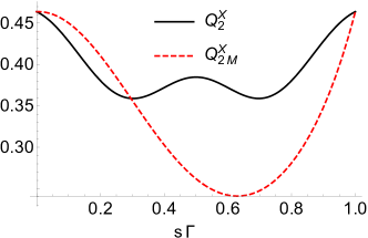
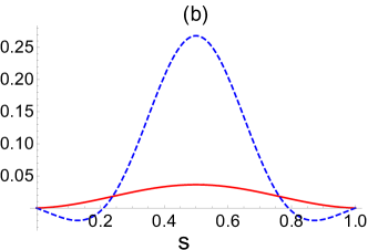
Figure 5: a) Comparison of the two-time probability distribution as a function of the first time s, for the exact formula (solid, black line) and the 2M statistics (dashed, red line). b) Violation of 2CL ($K_{+}(t,s)$) (dashed, blue line) and violation of NCGD ($N(t,s)$) (solid, red line). For both plots the environmental distribution is given by a sum of two Gaussians, with (in arbitrary units) $A_{\theta}=\sigma=p_{1}=t=1$, $p_{2}=2p_{1}$, $s\in[0,t]$.

In order for the statistics to be 2-CL, the following condition must hold

$$K_{+}(t,s) = \frac{1}{4}\Re[k(t-2s)-k(t)]$$ (43)

$$= \frac{e^{-2\sigma^{2}(t-2s)^{2}}}{4(A_{\theta}+1)}\left[\cos(2p_{1}(t-2s))+A_{\theta}\cos(2p_{2}(t-2s))\right]$$

$$+\frac{e^{-2\sigma^{2}t^{2}}}{4(A_{\theta}+1)}\left[\cos(2p_{1}t)+A_{\theta}\cos(2p_{2}t)\right]=0.$$

Furthermore, the model is CGD if [see Eq.(34)] the quantity

$$N(t,s):=\frac{2\left|\Im\left[k(s)\right]\Im\left[k^{*}(s)k(t)\right]\right|}{4|k(s)|^{2}}$$ (44)

$$=\frac{1}{2(1+A_{\theta})\left|e^{2isp_{1}}+A_{\theta}e^{2isp_{2}}\right|^{2}}\left(e^{-2t^{2}\sigma^{2}}\left[\sin(2sp_{1})+A_{\theta}\sin(2sp_{2})\right]\right.$$

$$\left.\phantom{\frac{1}{1}}\times\left[\sin(2(s-t)p_{1})+A_{\theta}(A_{\theta}\sin(2(s-t)p_{2})-\sin(2tp_{1}-2sp_{2})+\sin(2sp_{1}-2tp_{2}))\right]\right)$$

is different from 0.

As can be seen in Fig.5 a), for the considered choice of parameters the dynamics is NM at instants different from $s=0.29$. This allows for the existence of scenarios where the possible classicality of the statistics is unrelated to the absence of coherences. As a matter of fact, at the specific instants $s=0.21$ and $s=0.79$, where QRT is not satisfied, one finds that $K_{+}(t,s)=0$ and $N(t,s)\neq 0$, implying that 2-CL holds together with CGD (Fig.5 b)). By investigation (not reported here) of the model at hand in a wide region of parameters, we also observe that there does not seem to be a threshold in the amount of CGD, above which the violation of 2CL is guaranteed.

References

- (1) A. Einstein, B. Podolsky, and N. Rosen, Phys. Rev. 47, 777 (1935).
- (2) E. Schrödinger, Naturwissenschaften 23, (1935).
- (3) J.S. Bell, Speakable and Unspeakable in Quantum Mechanics (Cambridge University Press, Cambridge, 1987).
- (4) A.J. Leggett and A. Garg, Phys. Rev. Lett. 54, 857 (1985).
- (5) A.J. Leggett, Found. Phys. 18 939 (1988).
- (6) S.F. Huelga, T.W. Marshall and E. Santos, Phys. Rev. A 52, R2497 (1995).
- (7) N. Lambert, C. Emary, Y.-N. Chen, and F. Nori, Phys. Rev. Lett. 105, 176801 (2010).
- (8) A. Palacios-Laloy, F. Mallet, F. Nguyen, P. Bertet, D. Vion, D. Esteve, and A. N. Korotkov, Nat. Phys. 6, 442 (2010).
- (9) G. Waldherr, P. Neumann, S. F. Huelga, F. Jelezko, and J. Wrachtrup, Phys. Rev. Lett. 107, 090401 (2011).
- (10) G. C. Knee, S. Simmons, E. M. Gauger, J. J. Morton, H. Riemann, N. V. Abrosimov, P. Becker, H.-J. Pohl, K. M. Itoh, M. L. Thewalt, G. A. D. Briggs, and S. C. Benjamin, Nat. Commun. 3, 606 (2012).
- (11) C.-M. Li, N. Lambert, Y.-N. Chen, G.-Y. Chen, and F. Nori, Sci. Rep. 2, 885 (2012)
- (12) J. Kofler and C. Brukner, Phys. Rev. A 87, 052115 (2013).
- (13) C. Emary, N. Lambert and F. Nori, Rep. Prog. Phys. 77, 016001 (2014)
- (14) Z.Q. Zhou, S.F. Huelga, C.F. Li, and G.C. Guo, Phys. Rev. Lett. 115, 113002 (2015).
- (15) L. Clemente and J. Kofler, Phys. Rev. Lett. 116, 150401 (2016).
- (16) A. Friedenberger and E. Lutz, Phys. Rev. A 95, 022101 (2017).
- (17) G. Gour and R.W. Spekkens New J. Phys. 10, 033023 (2008).
- (18) T. Baumgratz, M. Cramer, and M. B. Plenio, Phys. Rev. Lett. 113, 140401 (2014).
- (19) J. Åberg, Phys. Rev. Lett. 113, 150402 (2014).
- (20) B. Yadin, J. Ma, D. Girolami, M. Gu, and Vlatko Vedral, Phys. Rev. X 6, 041028 (2016).
- (21) A. Winter and D. Yang, Phys. Rev. Lett 116, 120404 (2016).
- (22) E. Chitambar and G. Gour, Phys. Rev. Lett. 117, 030401 (2016)
- (23) N. Killoran, F. E. S. Steinhoff, and M. B. Plenio, Phys. Rev. Lett. 116, 080402 (2016).
- (24) A. Streltsov, G. Adesso, and M.B. Plenio, Rev. Mod. Phys. 89, 041003 (2017).
- (25) Z.-W. Liu, X. Hu, and S. Lloyd, Phys. Rev. Lett. 118, 060502 (2017).
- (26) G.S. Engel, T.R. Calhoun, E.L. Read, T.K. Ahn, T. Mancal, Y.C. Cheng, R.E. Blankenship, and G.R. Fleming, Nature 446 782 (2007).
- (27) A. Ishizaki and G.R. Fleming, Proc. Natl Acad. Sci. 106, 17255 (2009).
- (28) A.W. Chin, J. Prior, R. Rosenbach, F. Caycedo-Soler, S.F. Huelga and M.B. Plenio, Nat. Phys. 9, 113 (2013).
- (29) S.F. Huelga and M.B. Plenio, Contem. Phys. 54, 181 (2013).
- (30) M.M. Wilde, J.M. McCracken, and A. Mizel, Proc. R. Soc. A 466, 1347 (2010).
- (31) J.S. Briggs and A. Eisfeld, Phys. Rev. E 83, 051911 (2011).
- (32) W.H. Miller, J. Chem. Phys. 136, 210901 (2012).
- (33) R. de J. León-Montiel and J. P. Torres, Phys. Rev. Lett. 110, 218101 (2013).
- (34) E.J. O’Reilly and A. Olaya-Castro, Nat. Comm. 5, 3012 (2014).
- (35) W. Feller, An Introduction to Probability Theory and its Applications (Wiley, New York, 1971).
- (36) H.-P. Breuer and F. Petruccione, The Theory of Open Quantum Systems (Oxford University Press, New York, 2002).
- (37) M. Lax, Phys. Rev. 172, 350 (1968).
- (38) N.G. van Kampen, Stochastic Processes in Physics and Chemistry (North-Holland, Amsterdam,1992).
- (39) H. Carmichael, An Open Systems Approach to Quantum Optics (Springer-Verlag, Berlin, 1993).
- (40) C. W. Gardiner and P. Zoller, Quantum Noise: A Handbook of Markovian and Non-Markovian Quantum Stochastic Methods with Applications to Quantum Optics (Springer, Berlin, 2004).
- (41) G. Lindblad, Comm. Math. Phys. 65, 281 (1979).
- (42) L. Accardi, A. Frigerio, and J.T. Lewis, Publ. RIMS, Kyoto Univ. 18, 97 (1982).
- (43) G. Chiribella, G. M. D’Ariano, and P. Perinotti, Phys. Rev. Lett. 101, 060401 (2008).
- (44) S. Milz, F. Sakuldee, F.A. Pollock, and Kavan Modi, arXiv:1712.02589 (2017).
- (45) J.J. Halliwell, Phys. Rev. A 96, 012121 (2017).
- (46) S. Swain, J. Phys. A: Math. Gen. 14, 2577 (1981).
- (47) G. Guarnieri, A. Smirne, and B. Vacchini, Phys. Rev. A 90, 022110 (2014).
- (48) P. Talkner, Ann. Phys. 167, 390 (1986).
- (49) G.W. Ford and R. F. O’Connell, Phys. Rev. Lett. 77, 798 (1996).
- (50) E. B. Davies, Commun. Math. Phys. 39, 91 (1974); Math. Ann. 219, 147 (1976).
- (51) V. Gorini and A. Kossakowski, J. Math. Phys. 17, 1298 (1976); A. Frigerio and V. Gorini, ibid. 17, 2123 (1976).
- (52) M. Ban, Phys. Lett. A 381, 2313 (2017).
- (53) G. Lindblad, Commun. Math. Phys. 48, 119 (1976); V. Gorini, A. Kossakowski and E.C.G. Sudarshan, J. Math. Phys. 17, 821 (1976).
- (54) C.H. Fleming and B.L. Hu, Ann. of Phys. 327, 1238 (2011).
- (55) N. Lo Gullo, I. Sinayskiy, Th. Busch and F. Petruccione, arXiv: 1401.1126 (2014).
- (56) A. Rivas, S. F. Huelga, and M. B. Plenio, Rep. Prog. Phys. 77, 094001 (2014).
- (57) H.P. Breuer, E.M. Laine, J. Piilo, and B. Vacchini, Rep. Mod. Phys. 88, 021002 (2016).
- (58) Here for simplicity we identify Markovian statistics with the time-homogeneous Breuer2002 Markovian ones; in App.E we also present the time-inhomogeneous Markovian statistics.
- (59) From now on, we drop the subfix .
- (60) G. Lindblad, Response of Markovian and non-Markovian quantum stochastic systems to time-dependent forces, preprint, Stockholm, 1980.
- (61) A. Montina, Phys. Rev. Lett. 108, 160501 (2012).
- (62) D. Frustaglia, J.P. Baltanás, M.C. Velázquez-Ahumada, A. Fernández-Prieto, A. Lujambio, V. Losada, M.J. Freire, and A. Cabello, Phys. Rev. Lett. 116, 250404 (2016).
- (63) A. Cabello, M. Gu, O. Güne, Z.-P. Xu, Phys. Rev. Lett. 120, 130401 (2018).
- (64) B. Vacchini, A. Smirne, E.-M. Laine, J. Piilo, and H.-P. Breuer, New J. Phys. 13, 093004 (2011).
- (65) B. H. Liu, L. Li, Y.-F. Huang, C.-F. Li, G.-C. Guo, E.-M. Laine, H.-P. Breuer, and J. Piilo, Nat. Phys. 7, 931 (2011).
- (66) C. Arenz, R. Hillier, M. Fraas, and D. Burgarth, Phys. Rev. A 92, 022102 (2015); C. Arenz, D. Burgarth, P. Facchi, and R. Hillier, J. Math. Phys. 59, 032203 (2017).
- (67) Quite remarkably, the QRT does hold for a Lorentzian distribution if we consider its formulation for the two-time correlation functions of the system’s observables Guarnieri2014 , rather than for the statistics associated with projective measurements.