Explicit Inverse Confluent Vandermonde Matrices with Applications to Exponential Quantum Operators

Abstract

The Cayley-Hamilton problem of expressing functions of matrices in terms of only their eigenvalues is well-known to simplify to finding the inverse of the confluent Vandermonde matrix. Here, we give a highly compact formula for the inverse of any matrix, and apply it to the confluent Vandermonde matrix, achieving in a single equation what has only been achieved by long iterative algorithms until now. As a prime application, we use this result to get a simple formula for explicit exponential operators in terms of only their eigenvalues, with an emphasis on application to finite discrete quantum systems with time dependence. This powerful result permits explicit solutions to all Schrödinger and von Neumann equations for time-commuting Hamiltonians, and explicit solutions to any degree of approximation in the non-time-commuting case. The same methods can be extended to general finite discrete open systems to get explicit quantum operations for time evolution using effective joint systems, and the exact solution of all finite discrete Baker-Campbell-Hausdorff formulas.

I Introduction and Main Results

An important problem encountered in many situations is to find an exact expression for any analytic function $f(x)\equiv\sum\nolimits_{j=0}^{\infty}a_{j}x^{j}$ of an $n\times n$ matrix $A$ as $f(A)$ in terms of only the eigenvalues of $A$. While this problem has already been solved through the Cayley-Hamilton theorem Ham (1853); Hamilton (1862a, b, c); Cayley (1858); Frobenius (1878); Cayley (1889), its solution requires an explicit form of the inverse confluent Vandermonde matrix. In this work, we present a compact, exact form for the inverse confluent Vandermonde, thus explicitly solving all analytical functions of $n\times n$ operators as $f(A)$. While many others have found solutions to this problem Gautschi (1962); Hou and Pang (2002); Luther and Rost (2004); Hou and Hou (2007); Soto-Eguibar and Moya-Cessa (2011), the solution presented here is more compact and easily implemented.

As our focus for applications, we compute exponential operators in all cases of finite-dimensional $A$, including time-dependent and non-time-commuting $A$. Exponential operators are of prime importance in many fields, the simplest cases arising from the equation of motion $\partial_{t}\mathbf{x}(t){\kern-0.8pt}={\kern-0.8pt}A\mathbf{x}(t)$, where $\partial_{t}{\kern-0.8pt}\equiv{\kern-0.8pt}\frac{\partial}{{\partial t}}$, with solution $\mathbf{x}(t){\kern-0.8pt}\equiv{\kern-0.8pt}\mathbf{x}(t,t_{0})$ subject to initial condition $\mathbf{x}(t_{0})$, and operator $A$, represented by a complex-valued $n{\kern-0.8pt}\times{\kern-0.8pt}n$ matrix. For constant $A$, the well-known solution is $\mathbf{x}(t){\kern-0.9pt}={\kern-0.9pt}e^{\textnormal{\raisebox{-0.5pt}[-0.5pt][-0.5pt]{$(t-t_{0})A$}}}\mathbf{x}(t_{0})$, thus requiring exponential operator $e^{\textnormal{\raisebox{-0.5pt}[-0.5pt][-0.5pt]{$(t-t_{0})A$}}}$​. A key example is the Schrödinger equation $\partial_{t}|\psi(t)\rangle{\kern-0.8pt}={\kern-2.0pt}-{\kern-0.4pt}\frac{i}{\hbar}H|\psi(t)\rangle$ Schrödinger (1926a, b).

For the most general operator-function problem, given an $n\times n$ square matrix $A$, with $M$ distinct eigenvalues $\bm{\lambda}\equiv(\lambda_{1},\ldots,\lambda_{M})$ where $1\leq M\leq n$, so that $M\equiv\text{dim}(\bm{\lambda})$, with multiplicities $\bm{\mu}\equiv(\mu_{1},\ldots,\mu_{M})$ such that $\sum\nolimits_{\textnormal{\raisebox{0.3pt}[0.3pt][0.3pt]{$k\!=\!1$}}}^{\textnormal{\raisebox{-0.7pt}[-0.7pt][-0.7pt]{$M$}}}\mu_{k}=n$, for any analytic function $f(x)\equiv\sum\nolimits_{j=0}^{\infty}a_{j}x^{\textnormal{\raisebox{-0.3pt}[-0.3pt][-0.3pt]{$j$}}}$, we can obtain the operator function $f(A)$ as

$$f(A)=\sum\limits_{k=1}^{n}{b_{k}A^{k-1}},$$ (1)

with $A^{0}=I$, and scalars $b_{k}$ given by elements of vector

$$\mathbf{b}=V^{-1}\widetilde{\mathbf{f}},\;\;\;\text{where}\;\;\;\widetilde{f}_{c_{\alpha,\beta}}\equiv f^{(\beta-1)}(x)|_{\lambda_{\alpha}},$$ (2)

where $\mathbf{b}\equiv(b_{\textnormal{\raisebox{0.7pt}[0.7pt][0.7pt]{$1$}}},\ldots,b_{\textnormal{\raisebox{0.7pt}[0.7pt][0.7pt]{$n$}}})^{T}$, $\widetilde{\mathbf{f}}\equiv(\widetilde{f}_{1},\ldots,\widetilde{f}_{n})^{T}$, and $f^{(m)}(x)|_{\textnormal{\raisebox{0.7pt}[0.7pt][0.7pt]{$y$}}}{\kern-0.6pt}\equiv{\kern-0.6pt}({\textstyle{{d^{\textnormal{\raisebox{-2.0pt}[-2.0pt][-2.0pt]{$m$}}}{\kern 0.4pt}f{\kern 0.6pt}(x)}\over{dx^{m}}}})|_{\textnormal{\raisebox{0.7pt}[0.7pt][0.7pt]{$x{\kern-1.0pt}={\kern-1.0pt}y$}}}$, with indical register function $c_{\alpha,\beta}\equiv(\sum\nolimits_{j=1}^{\textnormal{\raisebox{-0.7pt}[-0.7pt][-0.7pt]{$\alpha{\kern-1.0pt}-{\kern-1.0pt}1$}}}{\mu_{j}}){\kern-0.5pt}+{\kern-0.5pt}\beta$ for $\alpha{\kern-0.5pt}\in{\kern-0.5pt}1,\ldots,M$ and $\beta{\kern-0.5pt}\in{\kern-0.5pt}1,\ldots,\mu_{\alpha}$, and confluent Vandermonde matrix $V$, with elements

$$V_{c_{\alpha,\beta},d}\equiv\partial_{\lambda_{\alpha}}^{\beta-1}\lambda_{\alpha}^{d-1}=\left\{{\begin{array}[]{*{20}l}0;&{d<\beta}\\ {\frac{{(d-1)!}}{{(d-\beta)!}}\lambda_{\alpha}^{d-\beta};}&{d\geq\beta.}\\ \end{array}}\right.$$ (3)

Due to the appearance of $V^{-1}$ in (2), the problem of (1) reduces to finding an explicit form for $V^{-1}$. Several formulas for this have already been discovered Gautschi (1962); Hou and Pang (2002); Luther and Rost (2004); Hou and Hou (2007); Soto-Eguibar and Moya-Cessa (2011), but they are generally recursive, algorithmic, and not compact, often taking many pages to describe. Here, we give a relatively simple expression for $V^{-1}$ in terms of $V$ as

$$V^{-1}{\kern-0.5pt}=\frac{{\frac{{(-1)^{n+1}}}{{n+1}}{\kern-0.5pt}\sum\limits_{k=1}^{n}{V^{k-1}{\kern-0.5pt}\sum\limits_{j=0}^{n}{e^{i\frac{{2\pi}}{{n+1}}jk}\det(e^{-i\frac{{2\pi}}{{n+1}}j}I{\kern-0.5pt}-{\kern-0.5pt}V)}}}}{{\det(V)}},$$ (4)

where $i{\kern-0.5pt}\equiv{\kern-0.5pt}\sqrt{-1}$, and the dependency on eigenvalues of $A$ is seen by putting (3) into (4). See App.A for a derivation of (4). Note that (4) holds for any $n$-level square matrix $V$ for which $\text{det}(V){\kern-0.5pt}\neq{\kern-0.5pt}0$, so it is also a general closed form for the inverse of a matrix. For the confluent Vandermonde $V$, $\text{det}(V){\kern-0.5pt}\neq{\kern-0.5pt}0$ always, and we can get $V^{-1}$ in terms of either elements of $V$ or eigenvalues $\bm{\lambda}$ of $A$, as shown in App.B. See App.C for a symbolic-software-friendly $V^{-1}$ without the complex exponentials.

The benefits of (4) over other matrix inverse forms are that (4) does not require recursive determinants of submatrices [see (7)], and it has no constrained indices, unlike other forms such as those involving Bell polynomials. Thus, (4) may be easier to use when we need to see the eigenvalues $\bm{\lambda}$ of $A$ or the elements of $V$ in $V^{-1}$ explicitly.

This closed form in (4) is just the definition of a matrix inverse with discrete Fourier orthogonality applied to the Cayley-Hamilton theorem’s formula Ham (1853); Hamilton (1862a, b, c); Cayley (1858); Frobenius (1878); Cayley (1889) (see App.A) for the adjugate of a matrix. Compartmentalizing,

$$V^{-1}=\frac{\text{adj}(V)}{\det(V)};\;\;\text{adj}(V)=(-1)^{n+1}\sum\limits_{k=1}^{n}{c_{k}V^{k-1}},$$ (5)

where the coefficients in the adjugate $\text{adj}(V)$ are

$$c_{k}=\frac{1}{{n+1}}\sum\limits_{j=0}^{n}{e^{i\frac{{2\pi}}{{n+1}}jk}\det(e^{-i\frac{{2\pi}}{{n+1}}j}I-V)}.$$ (6)

Furthermore, the determinant of any $n\times n$ matrix $B$ is

$$\det(B)=\sum\limits_{k_{1},\ldots,k_{n}=1,\ldots,1}^{n,\ldots,n}{\!\!\!\!\!\!\!\!\!\varepsilon_{k_{1},\ldots,k_{n}}\prod\limits_{q=1}^{n}{B_{q,k_{q}}}},$$ (7)

where $\varepsilon_{k_{1},\ldots,k_{n}}$ is the Levi-Civita symbol Ricci and Levi-Civita (1901), given by

$$\varepsilon_{k_{1},\ldots,k_{n}}=\prod\limits_{a=1,b=a+1}^{n-1,n}\!\!\!\!\!\!\!{{\mathop{\rm sgn}}(k_{b}-k_{a})}.$$ (8)

Thus, (7) and (8) show that we can indeed express (4) explicitly in terms of the elements of $V$ and therefore also in terms of the $\bm{\lambda}$ of $A$ from (3) (see App.B).

As our main example, we use $f(A){\kern-0.5pt}={\kern-0.5pt}e^{tA}$ for scalar $t$, a function of much interest Moler and Loan (1978, 2003); Luther and Rost (2004); Curtright et al. (2014); Curtright (2015), given here by (1) as

$$e^{tA}=\sum\limits_{k=1}^{n}{A^{k-1}\sum\limits_{\alpha=1}^{M}{\sum\limits_{\beta=1}^{\mu_{\alpha}}{(V^{-1})_{k,c_{\alpha,\beta}}t^{\beta-1}e^{\lambda_{\alpha}t}}}},$$ (9)

with $V^{-1}$ from (4) and $c_{\alpha,\beta}$ from (2). For $A\neq A(t)$, (9) solves $\partial_{t}\mathbf{x}(t)=A\mathbf{x}(t)$ as mentioned earlier, but (9) is true in general, regardless of any variables in $A$ (dependencies would only affect which differential equations it solves).

We will elaborate on the many uses of (9) in Sec.II, but for now we list a few special cases that arise due to particular eigenvalue conditions.

I.1 Special Case of $n$ Distinct Eigenvalues

When $A$ has all $n$ eigenvalues different from each other $\lambda_{1}\neq\cdots\neq\lambda_{n}$ so that $M=n$ and $\bm{\mu}=(1_{1},\ldots,1_{n})$, then the elements of the inverse confluent Vandermonde are

$$V_{a,b}^{-1}=\frac{{(-1)^{n-a}e_{n-a}(\{\bm{\lambda}\}\backslash\lambda_{b})}}{{\prod\limits_{c=1\neq b}^{n}\!\!{(\lambda_{b}-\lambda_{c})}}},$$ (10)

where the notation $\{\bm{\lambda}\}\backslash\lambda_{b}$ means all distinct eigenvalues except $\lambda_{b}$ (so $\text{dim}(\{\bm{\lambda}\}\backslash\lambda_{b}){\kern-0.8pt}={\kern-0.8pt}n{\kern-0.4pt}-{\kern-0.4pt}1$), and $e_{j}(\mathbf{x})$ are elementary symmetric polynomials of $m$ variables, given by

$$e_{j}(\mathbf{x})\equiv\left\{{\begin{array}[]{*{20}l}{1;}&{j=0}\\ {\sum\limits_{1\leq k_{1}<\cdots<k_{j}\leq m}\!\!\!\!\!\!\!\!\!\!\!\!\!{x_{k_{1}}\cdots x_{k_{j}}};}&{j\in 1,\ldots,m}\\ {0;}&{j>m,}\\ \end{array}}\right.$$ (11)

where $m\equiv\text{dim}(\mathbf{x})$. An easier form to implement may be

$$e_{j}(\mathbf{x})=\frac{{(-1)^{j}}}{{m+1}}\sum\limits_{k=0}^{m}{e^{i\frac{{2\pi}}{{m+1}}k(m-j)}\prod\limits_{l=1}^{m}{(e^{-i\frac{{2\pi}}{{m+1}}k}-x_{l})}},$$ (12)

for $j\in 0,\ldots,m$ and $m\equiv\text{dim}(\mathbf{x})$, derived in App.D. See App.C for a symbolic-software-friendly version of $e_{j}(\mathbf{x})$. Using (10) in (9) gives the $n$-distinct case of (9) as

$$e^{tA}=\sum\limits_{k=1}^{n}{A^{k-1}\sum\limits_{\alpha=1}^{n}{\frac{{(-1)^{n-k}e_{n-k}(\{\bm{\lambda}\}\backslash\lambda_{\alpha})}}{{\prod\limits_{c=1\neq\alpha}^{n}{\!\!(\lambda_{\alpha}-\lambda_{c})}}}e^{\lambda_{\alpha}t}}}.$$ (13)

I.2 Special Case of $n$ Degenerate Eigenvalues

When all $n$ eigenvalues of $A$ are the same $\lambda_{1}=\cdots=\lambda_{n}$ so that $M=1$ and $\bm{\mu}=(n)$, then $V^{-1}$ has elements

$$\begin{array}[]{*{20}l}{V_{a,b}^{-1}}&\!\!{=\frac{{V_{a,b}(-\lambda_{1})}}{{V_{a,a}V_{b,b}}}}&\!\!{=\left\{{\begin{array}[]{*{20}l}{0;}&{b<a}\\ {\frac{{(-\lambda_{1})^{b-a}}}{{(b-a)!(a-1)!}};}&{b\geq a.}\\ \end{array}}\right.}\\ \end{array}$$ (14)

Using (14) in (9) gives the $n$-degenerate case of (9) as

$$e^{tA}=e^{\lambda_{1}t}\sum\limits_{k=0}^{n-1}{\frac{{(tA)^{k}}}{{k!}}\sum\limits_{\beta=0}^{n-k-1}{\frac{{(-\lambda_{1}t)^{\beta}}}{{\beta!}}}},$$ (15)

where, whether the eigenvector matrix $U$ of $A$ is unitary or not, since $A=U\lambda_{1}IU^{-1}=\lambda_{1}I$, we get $e^{tA}\propto I$ as

$$\begin{array}[]{*{20}l}{e^{tA}}&\!\!{=\left({e^{\lambda_{1}t}\sum\limits_{k=0}^{n-1}{\frac{{(\lambda_{1}t)^{k}}}{{k!}}\sum\limits_{\beta=0}^{n-k-1}{\frac{{(-\lambda_{1}t)^{\beta}}}{{\beta!}}}}}\right)I=e^{\lambda_{1}t}I,}\\ \end{array}$$ (16)

and the unique eigenvalue of $e^{tA}$ is $e^{\lambda_{1}t}$. This also yields the identity $\sum\nolimits_{a=0}^{m}{\frac{{z^{a}}}{{a!}}\sum\nolimits_{b=0}^{m-a}{\frac{{(-z)^{b}}}{{b!}}}}=1$, for $m\in 0,\ldots,\infty$.

I.3 Intermediate Cases

In general, (9) with input from (4) constructed using (3) solves all cases of $e^{tA}$, for any multiplicity structure.

For a given $n$, the number of different cases of multiplicities is given by the partition function $p(n)$, the number of ways of writing any integer $n$ as a sum of positive integers ignoring summand order, given by Euler’s recursion formula Euler (1753); Skiena (1990) (modified here to accept all $n$),

$$p(n)=\delta_{n,0}+\sum\limits_{k=1}^{n}{(-1)^{k+1}[p(q_{n,k}^{+})+p(q_{n,k}^{-})]},$$ (17)

where $q_{n,k}^{\pm}\equiv n-\frac{1}{2}k(3k\pm 1)$, and by its definition $p(n<0)=0$, and by convention $p(0)\equiv 1$.

For example, for $n=4$, $\bm{\mu}$ can be $\bm{\mu}{\kern-0.7pt}={\kern-0.7pt}(1,1,1,1)$, $\bm{\mu}{\kern-0.7pt}={\kern-0.7pt}(1,1,2)$, $\bm{\mu}{\kern-0.7pt}={\kern-0.7pt}(2,2)$, $\bm{\mu}{\kern-0.7pt}={\kern-0.7pt}(1,3)$, or $\bm{\mu}{\kern-0.7pt}={\kern-0.7pt}(4)$, so that $\bm{\lambda}^{\prime}{\kern-0.7pt}={\kern-0.7pt}(\lambda_{1},\lambda_{2},\lambda_{3},\lambda_{4})$, $\bm{\lambda}^{\prime}{\kern-0.7pt}={\kern-0.7pt}(\lambda_{1},\lambda_{2},\lambda_{3},\lambda_{3})$, $\bm{\lambda}^{\prime}{\kern-0.7pt}={\kern-0.7pt}(\lambda_{1},\lambda_{1},\lambda_{2},\lambda_{2})$, $\bm{\lambda}^{\prime}{\kern-0.9pt}={\kern-0.9pt}(\lambda_{1},\lambda_{2},\lambda_{2},\lambda_{2})$, or $\bm{\lambda}^{\prime}{\kern-0.9pt}={\kern-0.9pt}(\lambda_{1},\lambda_{1},\lambda_{1},\lambda_{1})$, respectively, giving $p(4){\kern-1.1pt}={\kern-1.1pt}5$ cases, where $\bm{\lambda}^{\prime}{\kern-1.1pt}\equiv{\kern-1.1pt}({\lambda^{\prime}}_{\!1},\ldots,{\lambda^{\prime}}_{\!n})$ is the set of all eigenvalues including repetitions while the unprimed $\lambda_{k}$ are distinct eigenvalues. Since Sec.I.1 and Sec.I.2 give special forms for the two extreme cases, there are $p(n)-2$ cases left for each $n$ where further simple forms may exist. However, since $p(n)-2$ grows quickly with $n$, it may be generally easier to use (9) with (4).

II Important Applications

II.1 Time-Evolution Operations

A central task of quantum mechanics is to solve an equation of motion, such as the Schrödinger equation $\partial_{t}|\psi(t)\rangle{\kern-0.8pt}={\kern-2.0pt}-\!\frac{i}{\hbar}H|\psi(t)\rangle$ or the von Neumann equation $\partial_{t}\rho(t)=\!-[\frac{i}{\hbar}H,\rho(t)]$, for the quantum state of a system as function of time, given some Hamiltonian operator $H$ for the energy. For the von Neumann equation, states are represented as density operators $\rho(t)\equiv\rho(t,t_{0})\equiv|\psi(t)\rangle\langle\psi(t)|$ with the most general initial state being a mixture $\rho(t_{0})=\sum\nolimits_{j}{p_{j}|\psi_{j}(t_{0})\rangle\langle\psi_{j}(t_{0})|}$, where $\sum\nolimits_{j}{p_{j}}=1$ such that $p_{j}\in[0,1]$, and $|\psi_{j}(t_{0})\rangle$ are different pure states with $\langle\psi_{j}(t_{0})|\psi_{j}(t_{0})\rangle=1$, and $[A,B]\equiv AB-BA$.

Generally, the solution for all closed and some open systems has the form $\rho(t,t_{0})=U(t,t_{0})\rho(t_{0})U^{{\dagger}}(t,t_{0})$, or if the initial state is pure it may also be represented as $|\psi(t)\rangle=U(t,t_{0})|\psi(t_{0})\rangle$, where in both cases $U(t,t_{0})$ is the unitary time-evolution operator. Another popular similar equation of motion is the Heisenberg equation, where time-dependence is grouped with observables rather than the state, but in both Heisenberg and von Neumann pictures, all essential dynamics are contained in the Schrödinger equation for the time-evolution operator (SETEO) $\partial_{t}U(t,t_{0}){\kern-0.8pt}={\kern-1.0pt}-\frac{i}{\hbar}HU(t,t_{0})$.

More generally, all open-system time evolution can be expressed as quantum operations Hellwig and Kraus (1969, 1970); Choi (1975); Kraus (1983) of the form $\rho(t,t_{0})\!=\!\sum\nolimits_{k}E_{k}(t,t_{0})\rho(t_{0})E_{k}^{{\dagger}}(t,t_{0})$, where $E_{k}(t,t_{0})$ are time-dependent Kraus operators in the Hilbert space of the system, satisfying $\sum\nolimits_{k}\!E_{k}^{{\kern 0.1pt}{\dagger}}(t,t_{0})E_{k}(t,t_{0}){\kern-0.2pt}={\kern-0.2pt}I$. In this case, it is possible to find a larger effective joint closed system that evolves with a joint-system unitary of some effective joint-system Hermitian Hamiltonian Hedemann (2014). Therefore, we will focus only on unitary evolution operators here, since they can model open systems as just described.

Thus, we now show how to apply the exponential operator formulas of this paper to the three types of unitary time-evolution operators Sakurai (1994), followed by examples.

II.1.1 Time-Independent Hamiltonian

If $H\neq H(t)$, then the solution to the SETEO,

$$U(t,t_{0})=e^{-\frac{i}{\hbar}(t-t_{0})H},$$ (18)

is given explicitly by $e^{tA}$ from (9) with $t\to-\frac{i}{\hbar}(t-t_{0})$ and $A\to H$ with $n=\text{dim}(H)$, yielding (using $\Delta t\equiv t-t_{0}$),

$$U(t,t_{0})=\sum\limits_{k=1}^{n}{H^{k-1}\!\sum\limits_{\alpha=1}^{M}{\sum\limits_{\beta=1}^{\mu_{\alpha}}{V^{-1}_{k,c_{\alpha,\beta}}(-{\textstyle{i\over\hbar}}\Delta t)^{\beta-1}e^{-\frac{i}{\hbar}\lambda_{\alpha}\Delta t}}}},$$ (19)

where $\{\lambda_{\alpha}\}$ are now the distinct eigenvalues of $H$ (which are often known), and $M,\bm{\mu},c_{\alpha,\beta},V$ are as given in (1–4).

II.1.2 Time-Dependent, Time-Commuting Hamiltonian

If $H=H(t)$ and $[H(t),H(t^{\prime})]=0$ for $t\neq t^{\prime}$, then

$$U(t,t_{0})=e^{-\frac{i}{\hbar}\int_{t_{0}}^{t}{H(t^{\prime})dt^{\prime}}}$$ (20)

is given by $e^{tA}$ from (9) with $t\to-\frac{i}{\hbar}$ and $A\to\widetilde{H\rule{0.0pt}{7.5pt}}\equiv$ $\widetilde{H\rule{0.0pt}{7.5pt}}(t)\equiv\widetilde{H\rule{0.0pt}{7.5pt}}(t,t_{0})\equiv\int_{t_{0}}^{\textnormal{\raisebox{-0.6pt}[-0.6pt][-0.6pt]{$t$}}}{H(t^{\prime})dt^{\prime}}$ with $n=\text{dim}(H)$ so that

$$U(t,t_{0})=\sum\limits_{k=1}^{n}{[\widetilde{H}(t)]^{k-1}\!\sum\limits_{\alpha=1}^{M(t)}{\sum\limits_{\beta=1}^{\mu_{\alpha}^{(t)}}{\!V_{k,c_{\alpha,\beta}}^{-1(t)}(-{\textstyle{i\over\hbar}})^{\beta-1}e^{-\frac{i}{\hbar}\widetilde{\lambda}_{\alpha}^{(t)}}}}},$$ (21)

where we also put $\lambda_{\textnormal{\raisebox{0.7pt}[0.7pt][0.7pt]{$\alpha$}}}\!\to\!\widetilde{\lambda}_{\textnormal{\raisebox{0.7pt}[0.7pt][0.7pt]{$\alpha$}}}\!\equiv\!\widetilde{\lambda}_{\textnormal{\raisebox{0.7pt}[0.7pt][0.7pt]{$\alpha$}}}(t,t_{0})\!\equiv\!\widetilde{\lambda}_{\textnormal{\raisebox{0.7pt}[0.7pt][0.7pt]{$\alpha$}}}^{(t)}$ and $V^{-1}\to$ $V^{-1(t)}\!\equiv\!V^{-1}(\widetilde{\bm{\lambda}}^{\textnormal{\raisebox{-0.4pt}[-0.4pt][-0.4pt]{$(t)$}}})$, where $\widetilde{\bm{\lambda}}^{\textnormal{\raisebox{-0.4pt}[-0.4pt][-0.4pt]{$(t)$}}}\!\equiv\!(\widetilde{\lambda}_{1}^{\textnormal{\raisebox{0.4pt}[0.4pt][0.4pt]{$(t)$}}},\ldots,\widetilde{\lambda}_{M(t)}^{\textnormal{\raisebox{0.4pt}[0.4pt][0.4pt]{$(t)$}}})$ are the distinct eigenvalues of $\widetilde{H\rule{0.0pt}{7.0pt}}$ and can vary in time as can their multiplicities $\bm{\mu}^{\textnormal{\raisebox{-0.4pt}[-0.4pt][-0.4pt]{$(t)$}}}\!\equiv\!(\mu_{1}^{\textnormal{\raisebox{0.5pt}[0.5pt][0.5pt]{$(t)$}}}{\kern-1.0pt},\ldots,\mu_{M(t)}^{\textnormal{\raisebox{0.5pt}[0.5pt][0.5pt]{$(t)$}}})$ and their total number $M(t)$, where arguments are in superscripts to avoid confusing them as factors. Thus, at each time, the multiplicity structure of the eigenvalues of $\widetilde{H\rule{0.0pt}{7.5pt}}$ must be redetermined, and the structure of $V$ adapts accordingly.

II.1.3 Time-Dependent, Non-Time-Commuting Hamiltonian

If $H=H(t)$ and $[H(t),H(t^{\prime})]\neq 0$, then the Suzuki-Trotter formula Suzuki (1993) for time-ordered exponentials is

$$\begin{array}[]{*{20}l}{U(t,t_{0})}&\!\!{=\mathop{\lim}\limits_{N\to\infty}\prod\limits^{\leftarrow}{}_{r=1}^{N}e^{\frac{{-i}}{\hbar}H(t_{r})\Delta t_{N}}}\\ {}&\!\!{\approx e^{\frac{{-i}}{\hbar}H(t_{N})\Delta t_{N}}\!\cdots e^{\frac{{-i}}{\hbar}H(t_{2})\Delta t_{N}}e^{\frac{{-i}}{\hbar}H(t_{1})\Delta t_{N}}}\\ {}&\!\!{\approx U^{\prime}(t_{N},t_{N-1})\cdots U^{\prime}(t_{2},t_{1})U^{\prime}(t_{1},t_{0}),}\\ \end{array}$$ (22)

where the product’s arrow means it grows leftwards, and

$$\Delta t_{N}\!\equiv\!\Delta t_{N}(t)\!\equiv\!\frac{{t-t_{0}}}{N}\;\;\,\text{and}\;\;\,t_{r}\!\equiv\!t_{r}(t)\!\equiv\!t_{0}+r\Delta t_{N},$$ (23)

where $N\geq 1$ is as large as it needs to be for convergence, and $U^{\prime}(t_{r},t_{r-1})\equiv e^{-i(t_{r}-t_{r-1})H(t_{r})/\hbar}$.

Here, each factor of $e^{-iH(t_{r})\Delta t_{N}/\hbar}$ in (22) is given by $e^{tA}$ from (9) with $t\to-\frac{i}{\hbar}\Delta t_{N}$ and $A\to H(t_{r})$, so

$$\begin{array}[]{*{20}l}{U(t,t_{0})\approx}&\!\!\!{\prod\limits_{r=1}^{\scriptstyle\leftarrow\hfill\atop\scriptstyle N\hfill}{\left(\!{\rule{0.0pt}{14.0pt}}\right.\sum\limits_{k=1}^{n}{[H(t_{r})]^{k-1}}}}\\ {}&\!\!\!{\times\!\sum\limits_{\alpha=1}^{M(t_{r})}{\sum\limits_{\beta=1}^{\mu_{\alpha}^{(t_{r})}}{V_{k,c_{\alpha,\beta}}^{-1(t_{r})}(\frac{{-i}}{\hbar}\Delta t_{N})^{\beta-1}e^{\frac{{-i}}{\hbar}\lambda_{\alpha}^{(t_{r})}\Delta t_{N}}}}\left.{\rule{0.0pt}{14.0pt}}\!\!\!\!\right)\!,}\\ \end{array}$$ (24)

where $\lambda_{\alpha}\!\to\!\lambda_{\alpha}(t_{r}){\kern-0.6pt}\equiv{\kern-0.6pt}\lambda_{\alpha}^{(t_{r})}$, $V^{-1}\!\to\!V^{-1(t_{r})}\equiv V^{-1}(\bm{\lambda}^{\textnormal{\raisebox{-0.5pt}[-0.5pt][-0.5pt]{$(t_{r})$}}})$, and $\bm{\lambda}^{{\kern-0.9pt}(t_{r})}{\kern-0.7pt}\!\equiv\!{\kern-0.5pt}({\kern-0.5pt}\lambda_{{\kern-0.5pt}1}^{{\kern 1.2pt}\textnormal{\raisebox{-0.4pt}[-0.4pt][-0.4pt]{$(t_{r})$}}}{\kern-0.5pt}\!,\ldots,\!\lambda_{{\kern-0.5pt}M{\kern-0.7pt}(t_{r})}^{{\kern 0.5pt}\textnormal{\raisebox{0.3pt}[0.3pt][0.3pt]{$(t_{r})$}}})$ are the $M(t_{r})$ distinct eigenvalues of $H(t_{r})$, where $\bm{\mu}^{{\kern 0.7pt}\textnormal{\raisebox{-1.2pt}[-1.2pt][-1.2pt]{$(t_{r})$}}}\!\equiv\!(\mu_{{\kern-0.5pt}1}^{{\kern 1.2pt}\textnormal{\raisebox{0.3pt}[0.3pt][0.3pt]{$(t_{r})$}}}\!,\ldots,\mu_{{\kern-0.5pt}M{\kern-0.5pt}(t_{r})}^{\textnormal{\raisebox{0.3pt}[0.3pt][0.3pt]{$(t_{r})$}}}{\kern-0.5pt})$. Thus, we can get a symbolic expression for $U(t,t_{0})$ to any degree of approximation. Convergence is discussed in Sec.III.

This same procedure applies to general time-ordered exponentials $\tau\{e^{\textnormal{\raisebox{0.2pt}[0.2pt][0.2pt]{$\int_{t_{0}}^{t}{\kern-0.5pt}{A(t^{\prime})dt^{\prime}}$}}}\}$ where $\tau\{\cdot\}$ is the time ordering operator, with $\frac{-i}{\hbar}\to 1$ and $H(t_{r})\to A(t_{r})$ in (24). Time-ordered exponentials arise in many areas, such as in linearized quantum Langevin equations Gardiner and Collett (1985); Gardiner and Zoller (2010). See Giscard et al. (2015) for an intriguing method to get explicit time-ordered exponentials with path integrals.

II.1.4 Example: Exact Solution of All Single-Qubit Schrödinger and von Neumann Equations

For a single qubit, $n=2$, given a Hermitian Hamiltonian $H$, there are two multiplicity cases for eigenvalues of $H$; $\lambda_{1}\neq\lambda_{2}$ and $\lambda_{1}=\lambda_{2}$. If the time evolution of the system is unitary then there are three main cases.

Case 1: If $H\neq H(t)$, then in subcases where $\lambda_{1}\neq\lambda_{2}$,

$$\begin{array}[]{*{20}l}{U(t,t_{0})=}&\!\!{\frac{1}{{\lambda_{1}-\lambda_{2}}}\left[{(\lambda_{1}e^{\frac{{-i}}{\hbar}(t-t_{0})\lambda_{2}}-\lambda_{2}e^{\frac{{-i}}{\hbar}(t-t_{0})\lambda_{1}})I}\right.}\\ {}&\!\!{\left.{+(e^{\frac{{-i}}{\hbar}(t-t_{0})\lambda_{1}}-e^{\frac{{-i}}{\hbar}(t-t_{0})\lambda_{2}})H}\right],}\\ \end{array}$$ (25)

and in subcases where $\lambda_{1}=\lambda_{2}$,

$$U(t,t_{0})=e^{\frac{{-i}}{\hbar}(t-t_{0})H_{1,1}}I.$$ (26)

In both of the above subcases, since $n<5$, we can get the eigenvalues explicitly in terms of elements of $H$ as

$$\begin{array}[]{*{20}l}{\lambda_{\scriptstyle 1\hfill\atop\scriptstyle 2\hfill}}&\!\!{=\frac{{\text{tr}(H)}}{2}\pm\sqrt{(\frac{{\text{tr}(H)}}{2})^{2}-\det(H)}}\\ {}&\!\!{=\frac{{H_{1,1}+H_{2,2}\pm\sqrt{(H_{1,1}-H_{2,2})^{2}+4|H_{1,2}|^{2}}}}{2},}\\ \end{array}$$ (27)

in which case the condition $\lambda_{1}\neq\lambda_{2}$ becomes $H\neq H_{1,1}I$, and the condition $\lambda_{1}=\lambda_{2}$ becomes $H=H_{1,1}I$. Thus, putting (27) into (25) gives

$$U(t,t_{0})=e^{-{\textstyle{i\over\hbar}}(t-t_{0}){\textstyle{{H_{1,1}+H_{2,2}}\over 2}}}\!\left({\begin{array}[]{*{20}c}a&b\\ {-b^{*}}&{a^{*}}\\ \end{array}}\right)\!,$$ (28)

where $a$ and $b$ automatically obey $|a|^{2}\!+\!|b|^{2}\!=\!1$, given by

$$\begin{array}[]{*{20}l}a&\!\!{\equiv\cos(\omega_{H}\Delta t)-i\frac{{\Delta_{H}}}{{\hbar{\kern 0.5pt}\omega_{H}+\delta_{\omega_{H},0}}}\sin(\omega_{H}\Delta t)}\\ b&\!\!{\equiv-i\frac{{H_{1,2}}}{{\hbar{\kern 0.5pt}\omega_{H}+\delta_{\omega_{H},0}}}\sin(\omega_{H}\Delta t),}\\ \end{array}$$ (29)

with $\Delta t\equiv t-t_{0}$, and using abbreviations

$$\omega_{H}\equiv{\textstyle{1\over\hbar}}\sqrt{|\Delta_{H}|^{2}+|H_{1,2}|^{2}}\;\;\;\text{and}\;\;\;\Delta_{H}\equiv{\textstyle{{H_{1,1}-H_{2,2}}\over 2}},$$ (30)

and the $\delta_{\omega_{H},0}$ in (29) lets (28) hold for both multiplicities. Therefore, (28) exactly solves all Schrödinger and von Neumann equations for constant $H$. Thus, (28) lets us design any single-qubit unitary gate we want.

As an elementary example of gate design, to get a Hadamard gate $U_{H}=\frac{1}{{\sqrt{2}}}(_{1\;-1}^{1\;\;\;\,1})$, setting $U(t,t_{0})=U_{H}$ in (28) shows that, up to global phase, this can be exactly achieved with $H=\hbar(_{1\;-1}^{1\;\;\;\,1})$ at times $t=t_{0}+{\textstyle{1\over{\sqrt{2}}}}({\textstyle{\pi\over 2}}+2\pi k)$ for $k\in\{0,1,2,\ldots\}$. Similarly, a phase gate $U_{\phi}=(_{0\;\,e^{i\phi}}^{{\kern 0.5pt}1\;\;\;0})$ can be exactly achieved, up to global phase, by $H=\hbar(_{0\;-\Delta}^{\Delta\;\;\;0})$ with $\Delta>0$ at times $t=t_{0}+{\textstyle{1\over\Delta}}({\textstyle{\phi\over 2}}+2\pi k)$. Together, these two kinds of gates can be combined to produce arbitrary single-qubit gates.

Case 2: If $H=H(t)$ and $[H(t),H(t^{\prime})]=0$ for $t\neq t^{\prime}$, then $U(t,t_{0})$ is given by (25–30) with $(t-t_{0})\to 1$, $H\to\widetilde{H\rule{0.0pt}{7.0pt}}$, and $\lambda_{\alpha}\to\widetilde{\lambda}_{\alpha}^{(t)}$ where $\widetilde{H\rule{0.0pt}{7.0pt}}\equiv\widetilde{H\rule{0.0pt}{7.0pt}}(t,t_{0})\equiv\int_{t_{0}}^{t}{\!H(t^{\prime})dt^{\prime}}$ with distinct eigenvalues $\widetilde{\lambda}_{\alpha}^{(t)}$, which applied to (28), yields

$$U(t,t_{0})=e^{-{\textstyle{i\over\hbar}}{\textstyle{{\widetilde{H}_{1,1}+\widetilde{H}_{2,2}}\over 2}}}\!\left({\begin{array}[]{*{20}c}{\widetilde{a}}&{\widetilde{b}}\\ {-\widetilde{b}^{*}}&{\widetilde{a}^{*}}\\ \end{array}}\right)\!,$$ (31)

where (29) is likewise modified to give

$$\begin{array}[]{*{20}l}{\widetilde{a}}&\!\!{\equiv\cos(\omega_{\widetilde{H}})-i{\textstyle{{\Delta_{\widetilde{H}}}\over{\hbar\omega_{\widetilde{H}}+\delta_{\omega_{\widetilde{H}},0}}}}\sin(\omega_{\widetilde{H}})}\\ {\widetilde{b}}&\!\!{\equiv-i{\textstyle{{\widetilde{H}_{1,2}}\over{\hbar\omega_{\widetilde{H}}+\delta_{\omega_{\widetilde{H}},0}}}}\sin(\omega_{\widetilde{H}}),}\\ \end{array}$$ (32)

where $\omega_{\widetilde{H}}\equiv{\textstyle{1\over\hbar}}\sqrt{|\Delta_{\widetilde{H}}|^{2}+|\widetilde{H}_{1,2}|^{2}}$ and $\Delta_{\widetilde{H}}\equiv{\textstyle{{\widetilde{H}_{1,1}-\widetilde{H}_{2,2}}\over 2}}$.

Case 3: If $H=H(t)$ and $[H(t),H(t^{\prime})]\neq 0$, then in the $H\neq H_{1,1}I$ subcase, $U(t,t_{0})$ is given by (22), where each factor of the form $e^{-iH(t_{r})\Delta t_{N}/\hbar}$ is given by (28–30) with $(t-t_{0})\to\Delta t_{N}$, $H\to H(t_{r})$, where $\Delta t_{N}$ and $t_{r}$ are from (23), and $\lambda_{\alpha}\to\lambda_{\alpha}^{(t_{r})}$ are distinct eigenvalues of $H(t_{r})$, all of which, when put into (28) and then (22), yields

$$U(t,t_{0})\approx\prod\limits_{r=1}^{\scriptstyle\leftarrow\hfill\atop\scriptstyle N\hfill}{e^{-{\textstyle{i\over\hbar}}\Delta t_{N}{\textstyle{{H_{1,1}^{(t_{r})}+H_{2,2}^{(t_{r})}}\over 2}}}\!\left({\begin{array}[]{*{20}c}{a_{r}}&{b_{r}}\\ {-b_{r}^{*}}&{a_{r}^{*}}\\ \end{array}}\right)\!,}$$ (33)

where (29) is likewise modified to become

$$\begin{array}[]{*{20}l}{a_{r}}&\!\!{\equiv\cos(\omega_{H(t_{r})}\Delta t_{N})-i{\textstyle{{\Delta_{H(t_{r})}\sin(\omega_{H(t_{r})}\Delta t_{N})}\over{\hbar\omega_{H(t_{r})}+\delta_{\omega_{H(t_{r})},0}}}}}\\ {b_{r}}&\!\!{\equiv-i{\textstyle{{H_{1,2}^{(t_{r})}\sin(\omega_{H(t_{r})}\Delta t_{N})}\over{\hbar\omega_{H(t_{r})}+\delta_{\omega_{H(t_{r})},0}}}},}\\ \end{array}$$ (34)

s.t.$\omega_{H(t_{r})}\!\equiv\!{\textstyle{1\over\hbar}}\sqrt{|\Delta_{H(t_{r})}|^{2}\!+\!|H_{1,2}^{(t_{r})}|^{2}}$, $\Delta_{H(t_{r})}\!\equiv\!{\textstyle{{H_{1,1}^{(t_{r})}\!-\!H_{2,2}^{(t_{r})}}\over 2}}$. For details on the convergence of (33), see Sec.III.

When $H(t)=H_{1,1}(t)I$, the Hamiltonian is automatically time-commuting, and so even though we could use Case 3, an exact answer is assured more simply by using Case 2. For $n$-level systems, $U(t,t_{0})$ has a general hyperspherical form analogous to (28), as shown in Hedemann (2013).

Figure 1 plots the time evolution of a pure state on its Bloch sphere Bloch (1946); Nielsen and Chuang (2010), for the Hadamard and phase gate.

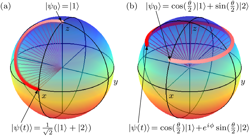
Figure 1: (color online) Exact evolution $|\psi(t)\rangle=U(t,t_{0})|\psi_{0}\rangle$ of a pure qubit with a constant Hamiltonian $H$ represented on the Bloch sphere, with the path colored to show the passage of time, with red as the final time. (a) shows the effects of $H=\hbar(_{1\;-1}^{1\;\;\;\,1})$ from $t_{0}$ to $t=t_{0}+{\textstyle{1\over{\sqrt{2}}}}{\textstyle{\pi\over 2}}$ at which time the Hadamard gate’s action is achieved, changing initial state $|\psi_{0}\rangle\!=\!|1\rangle$ into $|\psi(t)\rangle\!=\!\frac{1}{\sqrt{2}}(|1\rangle+|2\rangle)$. (b) shows the effects of $H=\hbar(_{0\;-\Delta}^{\Delta\;\;\;0})$ with $\Delta>0$ from $t_{0}$ to $t=t_{0}+{\textstyle{1\over\Delta}}{\textstyle{\phi\over 2}}$ where $\phi=0.85(2\pi)$ at which time the phase gate’s action is achieved, changing initial state $|\psi_{0}\rangle=\cos(\frac{\theta}{2})|1\rangle+\sin(\frac{\theta}{2})|2\rangle$ where $\theta=0.31\pi$ into $|\psi(t)\rangle=\cos(\frac{\theta}{2})|1\rangle+e^{i\phi}\sin(\frac{\theta}{2})|2\rangle$. Bloch coordinates are $(x,y,z)\!\equiv\!(2x_{1}x_{2},2x_{1}x_{3},2x_{1}^{2}{\kern-0.5pt}-{\kern-0.5pt}1)$, where $(x_{1},x_{2},x_{3})\!\equiv\!(\langle 1|\psi^{\prime}\rangle,\text{Re}[\langle 2|\psi^{\prime}\rangle],\text{Im}[\langle 2|\psi^{\prime}\rangle])$, with $|\psi^{\prime}\rangle\!\equiv\!e^{-i\arg[\langle 1|\psi(t)\rangle]}|\psi(t)\rangle$.

II.2 Baker-Campbell-Hausdorff (BCH) Formula

For operators $A$ and $B$ and scalar $s$, where $A$, $B$, and $s$ can be time-dependent, the BCH formula Sakurai (1994); Nielsen and Chuang (2010) is

$$\begin{array}[]{*{20}l}{e^{sA}Be^{-sA}}&\!\!{=\sum\limits_{k=0}^{\infty}{\frac{{s^{k}}}{{k!}}([A,)^{k}B(])^{k}}}\\ {}&\!\!{=B+s[A,B]+\frac{{s^{2}}}{{2!}}[A,[A,B]]+\cdots,}\\ \end{array}$$ (35)

where, for example, $([A,)^{0}B(])^{0}=B$, and $([A,)^{1}B(])^{1}=[A,B]$, and $([A,)^{2}B(])^{2}=[A,[A,B]]$, etc. The nested commutators in (35) are a common source of difficulty.

However, with our results, it is always possible to express this quantity exactly as a product of three matrices, $e^{sA}$, $B$, and $e^{-sA}$. In particular, in all cases of time-dependence, the explicit forms of $e^{\pm sA}$ are given by $e^{tA}$ from (9) with $t\to\pm s$, which leads to the finite sum,

$$\begin{array}[]{*{20}l}{e^{sA}Be^{-sA}{\kern-0.5pt}=}&\!\!{\kern-0.5pt}{\sum\limits_{k=1}^{n}{\!\!A^{k-1}B}\!\sum\limits_{\alpha=1}^{M}{}\!\sum\limits_{\beta=1}^{\mu_{\alpha}}{}\!\!V_{k,c_{\alpha,\beta}}^{-1}s^{\beta-1}e^{\lambda_{\alpha}s}}\\ {}&\!\!{\kern-0.5pt}{\times\!\!\sum\limits_{k^{\prime}=1}^{n}{\!\!\!A^{k^{\prime}-1}}\!\!\sum\limits_{\alpha^{\prime}=1}^{M}{}\!\sum\limits_{\beta^{\prime}=1}^{\mu_{\alpha^{\prime}}}{}\!\!V_{k^{\prime},c_{\alpha^{\prime},\beta^{\prime}}}^{-1}\!(-s)^{\beta^{\prime}-1}e^{-\lambda_{\alpha^{\prime}}s},}\\ \end{array}$$ (36)

where $A$ is allowed to be time-dependent, as are $s$ and $B$, $c_{\alpha,\beta}$ is as defined for (2), $n=\text{dim}(A)$, and $\lambda_{\alpha}$ are the distinct eigenvalues of $A$, all as in Sec.I. Thus, the computation of all the commutators can always be avoided and we always get an explicit solution, provided that we know the eigenvalues of $A$.

Note that the quantity $\tau{\kern-0.5pt}\{e^{\int_{t_{0}}^{t}{A(t^{\prime})dt^{\prime}}}\!\}B[\tau{\kern-0.5pt}\{e^{\int_{t_{0}}^{t}{A(t^{\prime})dt^{\prime}}}\!\}]^{{\dagger}}\!$, with time ordering operator $\tau\{\cdot\}$, is not solved by the BCH formula. However, in this case we can still solve this as a product of three operators, where $\tau\{e^{\textnormal{\raisebox{0.0pt}[0.0pt][0.0pt]{$\int_{t_{0}}^{t}{A(t^{\prime})dt^{\prime}}$}}}\}$ is approximated as an explicit function to any convergence for $N$ exponential operators, as in Sec.II.1.3, with the same convergence problems that all Suzuki-Trotter approximations have. However, such difficulties may be able to be avoided completely using effective joint systems, as mentioned in Sec.III.

II.3 Alternative Forms and General Examples

The version of $V^{-1}$ in (4) can be expressed (using parenthetical superscripts as arguments) as

$$\begin{array}[]{*{20}l}{V^{-1}=}&\!\!{\sum\nolimits_{l=1}^{n}\!{q_{l}^{(V)}V^{l-1}},}\\ \end{array}$$ (37)

with $\mathbf{q}^{(V)}\equiv(q_{1}^{(V)},\ldots,q_{n}^{(V)})^{T}$ where

$$\begin{array}[]{*{20}l}{\mathbf{q}^{(V)}\equiv W\mathbf{d}^{(V)};}&{\text{so}}&{q_{l}^{(V)}=\sum\nolimits_{m=1}^{n+1}\!{W_{l,m}}d_{m}^{(V)},}\\ \end{array}$$ (38)

where $\mathbf{d}^{(V)}\equiv(d_{1}^{(V)},\ldots,d_{n+1}^{(V)})^{T}$ and $W$ is an $n\times(n+1)$ matrix, each with elements

$$\begin{array}[]{*{20}l}{W_{l,m}}&\!\!{\equiv\frac{1}{{\sqrt{n+1}}}e^{i\frac{{2\pi}}{{n+1}}l(m-1)}}\\ {d_{m}^{(V)}}&\!\!{\equiv\frac{{(-1)^{n+1}}}{{\det(V)\sqrt{n+1}}}\det(e^{-i\frac{{2\pi}}{{n+1}}(m-1)}I-V),}\\ \end{array}$$ (39)

for $l\in 1,\ldots,n$ and $m\in 1,\ldots,n+1$, all of which allow (37) to compactly represent elements of $V^{-1}$ as $V_{a,b}^{-1}{\kern 0.0pt}={\kern-1.0pt}\sum\nolimits_{\textnormal{\raisebox{1.0pt}[1.0pt][1.0pt]{$l\!=\!1$}}}^{n}{q_{l}^{{\kern 1.0pt}\textnormal{\raisebox{0.0pt}[0.0pt][0.0pt]{$(V)$}}}(V^{\textnormal{\raisebox{-1.0pt}[-1.0pt][-1.0pt]{$l\!-\!1$}}})_{a,b}}{\kern 0.0pt}={\kern-2.0pt}\sum\nolimits_{\textnormal{\raisebox{1.0pt}[1.0pt][1.0pt]{$l\!=\!1$}}}^{n}{q_{l}^{{\kern 1.0pt}\textnormal{\raisebox{0.0pt}[0.0pt][0.0pt]{$(V)$}}}\langle a|V^{\textnormal{\raisebox{-1.0pt}[-1.0pt][-1.0pt]{$l\!-\!1$}}}|b\rangle}{\kern 0.0pt}{\kern-1.0pt}=$ $\sum\nolimits_{\textnormal{\raisebox{1.0pt}[1.0pt][1.0pt]{$l\!=\!1$}}}^{n}{{\kern 0.0pt}q_{l}^{{\kern 1.0pt}\textnormal{\raisebox{0.0pt}[0.0pt][0.0pt]{$(V)$}}}{\kern 0.0pt}\text{tr}(V^{\textnormal{\raisebox{-1.0pt}[-1.0pt][-1.0pt]{$l\!-\!1$}}}|b\rangle\langle a|})$ where $\{|1\rangle,\ldots,|n\rangle\}$ is the complete orthonormal standard basis.

Then, using the indical register function $c_{\alpha,\beta}$ from (2), we can express the general result from (1) as

$$\begin{array}[]{*{20}l}{f(A)}&\!\!{=\!\sum\limits_{k=1}^{n}{A^{k-1}\!\sum\limits_{\alpha=1}^{M}{\sum\limits_{\beta=1}^{\mu_{\alpha}}{V_{k,c_{\alpha,\beta}}^{-1}\widetilde{f}_{c_{\alpha,\beta}}}}}}\\ {}&\!\!{=\!\sum\limits_{k=1}^{n}{A^{k-1}\!\sum\limits_{\alpha=1}^{M}{\sum\limits_{\beta=1}^{\mu_{\alpha}}{\sum\limits_{l=1}^{n}{q_{l}^{(V)}(V^{l-1})_{k,c_{\alpha,\beta}}}\widetilde{f}_{c_{\alpha,\beta}}}}}}\\ {}&\!\!{=\!\sum\limits_{k=1}^{n}{A^{k-1}}\!\sum\limits_{l=1}^{n}{q_{l}^{(V)}\!\sum\limits_{\alpha=1}^{M}{\sum\limits_{\beta=1}^{\mu_{\alpha}}\!{(V^{l-1})_{k,c_{\alpha,\beta}}\widetilde{f}_{c_{\alpha,\beta}}}}},}\\ \end{array}$$ (40)

where $(V^{l-1})_{k,c_{\alpha,\beta}}\equiv\langle k|V^{l-1}|c_{\alpha,\beta}\rangle=\text{tr}(V^{l-1}|c_{\alpha,\beta}\rangle\langle k|)$, and $\widetilde{f}_{c_{\alpha,\beta}}$ is as in (2). Alternatively, we could use (60) in (1) to get $f(A)$ explicitly in terms of the eigenvalues of $A$, but (40) has the advantage of being more compact while still expressing $f(A)$ in terms of $V$ rather than its inverse. The benefit of expressing $f(A)$ with (1) and (4) rather than (40) is that (1) requires fewer auxiliary definitions, letting us see its dependence on $V$ more clearly.

Next, we give examples of $e^{tA}$ where $t$ is a scalar and $A$ is an $n\times n$ matrix with the same definition of distinct eigenvalue structure described in Sec.I.

In $n=2$, for $\bm{\mu}=(1,1)$,

$$\begin{array}[]{*{20}l}{e^{tA}}&\!\!{=\frac{1}{{\lambda_{1}-\lambda_{2}}}\left[{(\lambda_{1}e^{\lambda_{2}t}\!-\!\lambda_{2}e^{\lambda_{1}t})I\!-\!(e^{\lambda_{2}t}\!-\!e^{\lambda_{1}t})A}\right]\!,}\\ \end{array}$$ (41)

and for $\bm{\mu}=(2)$,

$$e^{tA}=e^{\lambda_{1}t}[(1-\lambda_{1}t)I+tA]=e^{\lambda_{1}t}I.$$ (42)

In $n=3$, for $\bm{\mu}=(1,1,1)$,

$$\begin{array}[]{*{20}l}{e^{tA}=}&\!\!{\frac{1}{{(\lambda_{1}-\lambda_{2})(\lambda_{1}-\lambda_{3})(\lambda_{2}-\lambda_{3})}}\left\{{[\lambda_{1}\lambda_{2}(\lambda_{1}-\lambda_{2})e^{\lambda_{3}t}-\lambda_{1}\lambda_{3}(\lambda_{1}-\lambda_{3})e^{\lambda_{2}t}+\lambda_{2}\lambda_{3}(\lambda_{2}-\lambda_{3})e^{\lambda_{1}t}]I}\right.}\\ {}&\!\!{\left.{+[-(\lambda_{1}^{2}-\lambda_{2}^{2})e^{\lambda_{3}t}+(\lambda_{1}^{2}-\lambda_{3}^{2})e^{\lambda_{2}t}-(\lambda_{2}^{2}-\lambda_{3}^{2})e^{\lambda_{1}t}]A+[(\lambda_{1}-\lambda_{2})e^{\lambda_{3}t}-(\lambda_{1}-\lambda_{3})e^{\lambda_{2}t}+(\lambda_{2}-\lambda_{3})e^{\lambda_{1}t}]A^{2}}\right\},}\\ \end{array}$$ (43)

for $\bm{\mu}=(1,2)$,

$$\begin{array}[]{*{20}l}{e^{tA}=}&\!\!{\frac{1}{{(\lambda_{1}-\lambda_{2})^{2}}}\left({\{\lambda_{1}[(\lambda_{1}-2\lambda_{2})-\lambda_{2}(\lambda_{1}-\lambda_{2})t]e^{\lambda_{2}t}+\lambda_{2}^{2}e^{\lambda_{1}t}\}I}\right.}\\ {}&\!\!{\left.{+\{[2\lambda_{2}+(\lambda_{1}^{2}-\lambda_{2}^{2})t]e^{\lambda_{2}t}-2\lambda_{2}e^{\lambda_{1}t}\}A+\{-[1+(\lambda_{1}-\lambda_{2})t]e^{\lambda_{2}t}+e^{\lambda_{1}t}\}A^{2}}\right),}\\ \end{array}$$ (44)

and for $\bm{\mu}=(3)$,

$$\begin{array}[]{*{20}l}{e^{tA}}&\!\!{=e^{\lambda_{1}t}[(1-\lambda_{1}t+\frac{1}{2}\lambda_{1}^{2}t^{2})I+(1-\lambda_{1}t)tA+\frac{1}{2}t^{2}A^{2}]}\\ {}&\!\!{=e^{\lambda_{1}t}I.}\\ \end{array}$$ (45)

As mentioned in Sec.I, these results also hold if $A$ is $t$-dependent, but such dependence will affect which differential equations are solved by $e^{tA(t)}$.

For excellent examples of the fully-distinct-eigenvalue exponentials, see Curtright et al. (2014) which gives the single-mode spin operators using a Cayley-Hamilton expansion as we have here. However, for exponentials of multipartite spin operators, there will generally be degeneracy in the eigenvalues, and in that case, the methods presented here are needed instead. Note that the examples in (41–45) are for dimensions that do not support multipartite systems, so for multipartite operators, use (9) or (40).

III Conclusions

We have provided a few new subtle improvements for achieving operator functions with Vandermonde methods. While these improvements are very simple, they allow great simplifications for these kinds of problems, particularly with theoretical work.

The main simple improvements are the new formula for the matrix inverse in (4) involving unit-complex exponentials, and the indical register function $c_{\alpha,\beta}$ defined for (2). The inverse function lets us express the inverse confluent Vandermonde $V^{-1}$ as a simple nonrecursive formula in terms of the confluent Vandermonde $V$ itself, without any constraints on the indices. Meanwhile, $c_{\alpha,\beta}$ automatically takes care of mapping the $n\times n$ indices of $V$ to the correct matrix elements based on its multiplicity structure. This allows all operator functions to be described as closed-form self-contained sums, as seen in the main example for exponential operators in (9).

The motivation for studying the inverse confluent Vandermonde matrix in particular is that it appears in the Cayley-Hamilton theorem for general operator functions, allowing any analytic function of an operator to be expressed only in terms of that operator’s eigenvalues and itself, without explicit appearance of its eigenvectors, which would be considerably more complicated.

The special-case formulas for elements of $V^{-1}$ in (10) and (14) were found by observation and confirmed exactly through symbolic testing for $n\in 2,\ldots,8$. The true usefulness of (4) really becomes apparent when we consider the intermediate cases of multiplicity, the number of which rapidly increases with $n$, as explained in Sec.I.3. In those cases, (4) provides a particularly simple form for $V^{-1}$, valid for all multiplicity structures.

Since exponential operators are of particular importance in quantum mechanics, we focused on that for our main examples. We showed how to get explicit forms of the time-evolution operator $U(t,t_{0})$ for the three main cases, with the non-time-commuting case being merely an approximation, but which can be achieved to any degree of accuracy, remaining symbolic in all cases.

To verify how well the approximation of (24) works for a given $H(t)$, $N$, and $\Delta t\equiv t-t_{0}$, (24) can be tested in both sides of the SETEO $\partial_{t}U(t,t_{0}){\kern-0.8pt}={\kern-1.0pt}-\frac{i}{\hbar}H(t)U(t,t_{0})$, to see how well their difference approximates the zero matrix. It is important to note that a SETEO test requires that we retain full symbolic $t$-dependence in $\Delta t_{N}$ and $t_{r}$ from (23) to get the correct $\partial_{t}U(t,t_{0})$. This test worked well for small dimensions $n$ and orders $N$ but when that is impractical, we must rely on tests showing that $H(t^{\prime})$ is approximately constant during $\Delta t_{N}(t^{\prime})$ for all $t^{\prime}\in[t_{0},t]$. Furthermore, convergence and stability depend strongly on the magnitudes of the eigenvalues of $H(t)$, which should ideally be less than unity.

However, despite any convergence difficulties that may arise with (24), the unitary dynamics of systems of non-time-commuting Hamiltonians may be able to be modeled as reductions of larger effective finite systems with constant or time-commuting Hamiltonians, and then the results of (19) or (21) can be used quite effectively.

In particular, we pointed out that, for Hamiltonian operators whose eigenvalues are known, which is often the case, this allows exact solution of all Schrödinger, von Neumann, and Heisenberg equations for finite quantum systems with unitary time evolution (the Heisenberg time evolution is also governed by $U(t,t_{0})$, but the solution for the expectation values of time-evolving observables is focused upon in that case, so $U(t,t_{0})$ is involved indirectly, yet still responsible for all dynamics).

For open quantum systems undergoing nonunitary time evolution, these results can still be used to find explicit formulas for the $U(t,t_{0})$ of finite-sized effective joint systems, which can then be partial-traced over to get the nonunitary dynamics of the system of interest, provided that such a system is finite-dimensional. While these results have already been worked out by the author, they are beyond the scope of the present discussion because they require much more space to explain. Therefore, that will be the subject of future work.

We also showed several other useful results such as an exact finite-term BCH formula in Sec.II.2, and several examples of general operator decompositions in Sec.II.3. Furthermore, we found a simple alternative form for elementary symmetric polynomials in (12).

The main reason it is important to achieve symbolic forms, in any field of study, is that optimization typically requires derivatives, and having a symbolic formula permits differentiation, whereas that information becomes much harder to glean from strictly numerical results.

In closing, it is hoped that although the results of this paper are somewhat elementary, they can nevertheless prove useful in many applications, saving time and effort in otherwise tedious calculations for operator functions. This may make tasks such as optimization of quantum systems significantly more approachable, and may even offer insights into many physical phenomena.

Appendix A Derivation of Compact Matrix Inverse Formula

From the Cayley-Hamilton theorem Ham (1853); Hamilton (1862a, b, c); Cayley (1858); Frobenius (1878); Cayley (1889), given $n\times n$ matrix $A$ with characteristic equation

$$p(\lambda)\equiv\det(\lambda I-A)\equiv\sum\limits_{k=0}^{n}{c_{k}\lambda^{k}}=0,$$ (46)

(unrelated to $p(n)$ of (17)), where expanding leads to a Viète’s formula Viète (1615); Girard (1629); Newton (1707),

$$c_{k}=(-1)^{n-k}e_{n-k}(\bm{\lambda}^{\prime}),\;\;\;k\in 0,\ldots,n,$$ (47)

where $e_{j}(\bm{\lambda}^{\prime})$ are elementary symmetric polynomials as in (11) and $\bm{\lambda}^{\prime}\equiv(\lambda_{1}^{\prime},\ldots,\lambda_{n}^{\prime})$ are all eigenvalues of $A$ including repetitions, the Cayley-Hamilton theorem’s main result is that (46) also holds with matrix argument $A$ as

$$p(A)=\sum\limits_{k=0}^{n}{c_{k}A^{k}}=0I.$$ (48)

Then, in the rightmost equation of (48), pulling out the first term, using $c_{0}=(-1)^{n}\det(A)$ from (47), multiplying through by $A^{-1}$, and solving for $A^{-1}$ gives

$$A^{-1}=\frac{\text{adj}(A)}{\det(A)};\;\;\;\text{adj}(A)\equiv(-1)^{n+1}\sum\limits_{k=1}^{n}{c_{k}A^{k-1}},$$ (49)

which defines the adjugate of $A$ as $\text{adj}(A)$, as seen in (5).

While Viète’s formula would give the $c_{k}$ in terms of $\bm{\lambda}^{\prime}$, we can get $c_{k}$ directly from $A$ using discrete Fourier orthonormality. Recall that the $n$-level discrete Fourier unitary matrix Nielsen and Chuang (2010) has elements

$$F_{j,l}\equiv F_{j,l}^{[n]}={\textstyle{1\over{\sqrt{n}}}}e^{-i{\textstyle{{2\pi}\over n}}(j-1)(l-1)}\;\;\text{for}\;\;j,l\in 1,\ldots,n.$$ (50)

Like all unitaries, since the Hermitian conjugate is the inverse $F^{{\dagger}}=F^{-1}$, we get orthonormality,

$$\sum\limits_{j=1}^{n}{F_{j,k}^{*}F_{j,l}}=\delta_{k,l}.$$ (51)

To relate the $c_{k}$ to $A$ itself, we will use (46), which has $n+1$ terms, so put $n\to n+1$ in (50) and (51), and shift the index as $j\to j+1$, which yields

$${\textstyle{1\over{n+1}}}\sum\limits_{j=0}^{n}{e^{i{\textstyle{{2\pi}\over{n+1}}}jk}e^{-i{\textstyle{{2\pi}\over{n+1}}}jl}}=\delta_{k,l}.$$ (52)

Now, if we put $\lambda\!=\!e^{-i2\pi j/(n+1)}$ in (46) as $p(e^{-i2\pi j/(n+1)})$ with new summation index $h$, and then multiply through by $e^{i2\pi jk/(n+1)}$, summing over $j$ from $0$ to $n$, and scaling by $\frac{1}{n+1}$ lets us use (52) to get

$$\begin{array}[]{*{20}r}{\sum\limits_{h=0}^{n}{c_{h}e^{-i{\textstyle{{2\pi}\over{n+1}}}jh}}=}&\!\!{\det(e^{-i{\textstyle{{2\pi}\over{n+1}}}j}I-A)}\\ {e^{i{\textstyle{{2\pi}\over{n+1}}}jk}\sum\limits_{h=0}^{n}{c_{h}e^{-i{\textstyle{{2\pi}\over{n+1}}}jh}}=}&\!\!{e^{i{\textstyle{{2\pi}\over{n+1}}}jk}p(e^{-i{\textstyle{{2\pi}\over{n+1}}}j})}\\ {\sum\limits_{h=0}^{n}{c_{h}\delta_{k,h}}=}&\!\!{\frac{1}{{n+1}}\sum\limits_{j=0}^{n}{e^{i{\textstyle{{2\pi}\over{n+1}}}jk}p(e^{-i{\textstyle{{2\pi}\over{n+1}}}j})}}\\ {c_{k}=}&\!\!{\frac{1}{{n+1}}\sum\limits_{j=0}^{n}{e^{i{\textstyle{{2\pi}\over{n+1}}}jk}p(e^{-i{\textstyle{{2\pi}\over{n+1}}}j})},}\\ \end{array}$$ (53)

where $p(e^{-i{\textstyle{{2\pi}\over{n+1}}}j})=\det(e^{-i{\textstyle{{2\pi}\over{n+1}}}j}I-A)$, which gives the result in (6). Although there are many other ways to get the $c_{k}$, this way is particularly compact and useful.

Thus, (53) allows direct computation of $\text{adj}(A)$ in (49), and together with the well-known formulas for the determinant and general Levi-Civita symbol given in (7) and (8), (49) then yields the final closed-form result for $A^{-1}$ in (4) (written in terms of matrix $V$ there), where $A^{-1}$ exists if and only if (iff) $\det(A)\neq 0$.

Thus, (4) can be used for any nonsingular $n\times n$ matrix $V$, not just confluent Vandermondes. While this result may seem trivially simple since algorithms are already well-known for the matrix inverse, keep in mind that many published papers have labored over the inverse of the confluent Vandermonde Gautschi (1962); Hou and Pang (2002); Luther and Rost (2004); Hou and Hou (2007); Soto-Eguibar and Moya-Cessa (2011), with the simplest results still taking many pages to explain, whereas here we have achieved it in a single equation simply by deriving a more compact formula for an arbitrary matrix inverse.

Appendix B Inverse Confluent Vandermonde in Terms of Eigenvalues of its Parent Matrix

First, to get the inverse confluent Vandermonde matrix $V^{-1}$ in terms of the elements of $V$ only (and not in terms of $V$ as a whole, as in (4)), first we need

$$\begin{array}[]{*{20}l}{V^{k-1}=}&\!\!{\sum\limits_{l,m=1,1}^{n,n}\!\!{\left({\,\sum\limits_{\mathbf{r}=\mathbf{1}}^{\mathbf{n}}{\delta_{r_{1},l}\delta_{r_{k},m}\prod\limits_{u=1}^{k-1}{V_{r_{u},r_{u+1}}}}\!}\right)\!|l\rangle\langle m|,}}\\ \end{array}$$ (54)

with vector indices $\mathbf{r}\equiv(r_{1},\ldots,r_{k})$, $\mathbf{1}\equiv(1_{1},\ldots,1_{k})$, $\mathbf{n}\equiv(n_{1},\ldots,n_{k})$, where $1_{j}\equiv 1$, $n_{j}\equiv n$, and $\{|1\rangle,\ldots,|n\rangle\}$ forms the complete orthonormal standard basis, and $\delta_{a,b}$ is the Kronecker delta. Next, using

$$(e^{-i{\textstyle{{2\pi}\over{n+1}}}j}I-V)_{z,h_{z}}=(e^{-i{\textstyle{{2\pi}\over{n+1}}}j}\delta_{z,h_{z}}-V_{z,h_{z}}),$$ (55)

where $z\in 1,\ldots n$ and $h_{z}\in 1,\ldots n$, together with (54) and (7) in (4) gives $V^{-1}$ in explicitly terms of $V_{a,b}$.

To get $V^{-1}$ explicitly in terms of the $M$ distinct eigenvalues $\bm{\lambda}\equiv(\lambda_{1},\ldots,\lambda_{M})$ of its parent matrix $A$ (the matrix whose eigenvalues define $V$ as given in Sec.I), we can either use (3) in (54) and (55), or we can adapt (3) as

$$V_{c_{\alpha,\beta},d}={\kern-1.0pt}\frac{{(d-1)!}\lambda_{\alpha}^{d-\beta}\text{sgn}(\delta_{d,\beta}\!+\!\text{max}{\{0,d-\beta\}})}{[(d-\beta)\text{sgn}(\delta_{d,\beta}\!+\!\text{max}{\{0,d-\beta\}})]!},$$ (56)

where $\alpha\in 1,\ldots,M$, $\beta\in 1,\ldots,\mu_{\alpha}$, $d\in 1,\ldots,n$, and $c_{\alpha,\beta}$ is defined after (2).

However, in (54–56) and (4), explicit calculation of elements of $V$ requires the inverse indical register function for $c_{\alpha,\beta}$, meaning: given some value $v$ in the range of $c_{\alpha,\beta}$, what are $\alpha$ and $\beta$? Thus, given $v\in 1,\ldots,n$, the values of $\alpha$ and $\beta$ for which $c_{\alpha,\beta}\equiv(\sum\nolimits_{j=1}^{\alpha-1}{\mu_{j}})+\beta=v$ for $\alpha\in 1,\ldots,M$ and $\beta\in 1,\ldots,\mu_{\alpha}$ are

$$\alpha\!=\!R_{v}\!\equiv\!\!\sum\limits_{a,b=1,1}^{M,\max\{\bm{\mu}\}}\!\!\!\!\!\!\!{a\delta_{v,c_{a,b}}}\;\;\;\text{and}\;\;\;\beta\!=\!C_{v}\!\equiv\!\!\sum\limits_{a,b=1,1}^{M,\max\{\bm{\mu}\}}\!\!\!\!\!\!\!{b\delta_{v,c_{a,b}}},$$ (57)

where $c_{a,b}\equiv(\,\sum\nolimits_{j=1}^{a-1}{\mu_{j}})+b$ and $\bm{\mu}\equiv(\mu_{1},\ldots,\mu_{M})$ as in Sec.I. Thus, (57) transforms (56) to

$$V_{q,d}={\kern-1.0pt}\frac{{(d-1)!}S_{d,C_{q}}}{{[(d-C_{q})S_{d,C_{q}}]!}}\lambda_{R_{q}}^{d-C_{q}},$$ (58)

for $q,d\in 1,\ldots,n$, with abbreviating function,

$$S_{z,y}\equiv{\mathop{\rm sgn}}(\delta_{z,y}+\max\{0,z-y\})=\left\{{\begin{array}[]{*{20}l}0;&\;{z<y}\\ 1;&\;{z\geq y,}\\ \end{array}}\right.$$ (59)

so now (58) gives elements of $V$ as a single-term function with no restrictions on its indices.

Putting everything together, we can now write $V^{-1}$ explicitly in terms of the distinct eigenvalues of its parent matrix $A$ by putting (58) into (54), (55), and (7), and putting all of those into (4), to get

$$V^{-1}=\frac{{\left(\!\begin{array}[]{l}\frac{{(-1)^{n+1}}}{{n+1}}\sum\limits_{k=1}^{n}{\left[{\sum\limits_{l,m=1,1}^{n,n}{\left({\sum\limits_{\mathbf{r}=\mathbf{1}}^{\mathbf{n}}{\delta_{r_{1},l}\delta_{r_{k},m}\prod\limits_{u=1}^{k-1}{\frac{{(r_{u+1}-1)!S_{r_{u+1},C_{r_{u}}}\lambda_{R_{r_{u}}}^{r_{u+1}-C_{r_{u}}}}}{{[(r_{u+1}-C_{r_{u}})S_{r_{u+1},C_{r_{u}}}]!}}}}}\right)|l\rangle\langle m|}}\right]}\\ \times\sum\limits_{j=0}^{n}{e^{i\frac{{2\pi}}{{n+1}}jk}}\sum\limits_{\mathbf{h}=\mathbf{1}}^{\mathbf{n}}{\left[{\left({\prod\limits_{x=1,y=x+1}^{n-1,n}\!\!\!\!\!\!\!\!\!{{\mathop{\rm sgn}}(h_{y}-h_{x})}}\right)\!\left({\prod\limits_{z=1}^{n}{\!(e^{-i\frac{{2\pi}}{{n+1}}j}\delta_{z,h_{z}}-\frac{{(h_{z}-1)!S_{h_{z},C_{z}}\lambda_{R_{z}}^{h_{z}-C_{z}}}}{{[(h_{z}-C_{z})S_{h_{z},C_{z}}]!}})}\!}\right)}\right]}\\ \end{array}\!\right)_{\,{}_{\,{}^{\,{}_{\,{}_{\,{}_{\,}}}}}\!\!\!\!\!\!\!}}}{{\sum\limits_{\mathbf{k}=\mathbf{1}}^{\mathbf{n}}{\left[{\left({\prod\limits_{a=1,b=a+1}^{n-1,n}\!\!\!\!\!\!\!\!\!{{\mathop{\rm sgn}}(k_{b}-k_{a})}}\right)\!\left({\prod\limits_{c=1}^{n}{\frac{{(k_{c}-1)!S_{k_{c},C_{c}}\lambda_{R_{c}}^{k_{c}-C_{c}}}}{{[(k_{c}-C_{c})S_{k_{c},C_{c}}]!}}}}\right)}\right]\rule{0.0pt}{19.0pt}}}},$$ (60)

where $i\equiv\sqrt{-1}$, $\mathbf{r}\equiv(r_{1},\ldots,r_{k})$, and $\{|1\rangle,\ldots,|n\rangle\}$ forms the complete orthonormal standard basis as in (54), and $\mathbf{h}\equiv(h_{1},\ldots,h_{n})$, $\mathbf{k}\equiv(k_{1},\ldots,k_{n})$, and $R_{v}$ and $C_{v}$ are given by (57), $S_{z,y}$ is given by (59), and $\mathbf{1}\equiv(1,\ldots,1)$ and $\mathbf{n}\equiv(n,\ldots,n)$ have dimensions $k$ or $n$ depending on their usage. Thus, (60) gives the inverse confluent Vandermonde $V^{-1}$ as an explicit function of the distinct eigenvalues of parent matrix $A$, in a single, nonrecursive equation that works for all multiplicity cases.

Appendix C Symbolic-Software-Friendly Inverse

Adapting the results from Macdonald (1979), given $\mathbf{x}=(x_{1},\ldots,x_{m})$, and $m\times m$ matrix $X$ with full set of eigenvalues $\mathbf{x}$ including repetitions, if we define the $j\times j$ matrix

$$Q^{[j]}\!\equiv\!\delta_{j,0}\!+\!\!\left({\sum\limits_{a=2}^{j}{\!(a\!-\!1)|a\!-\!1\rangle\langle a|}}\!\right)\!\!+\!\sum\limits_{q=1}^{j}{p_{q}\!\sum\limits_{b=q}^{j}{\!|b\rangle\langle b\!-\!q\!+\!1|,}}$$ (61)

where $\{|1\rangle,\ldots,|j\rangle\}$ is the standard basis and $p_{q}\equiv p_{q}(\mathbf{x})\equiv\sum\nolimits_{c=1}^{m}{x_{c}^{\textnormal{\raisebox{0.5pt}[0.5pt][0.5pt]{$q$}}}}$ are power sums, then two useful forms of the elementary symmetric polynomials are

$$\begin{array}[]{*{20}c}{e_{j}(\mathbf{x})\equiv{\textstyle{1\over{j!}}}\det(Q^{[j]}(\mathbf{x}))}&{\;\text{or}}&{e_{j}(X)\equiv{\textstyle{1\over{j!}}}\det(Q^{[j]}(X)),}\\ \end{array}$$ (62)

with $Q^{[j]}(\mathbf{x})\!\equiv\!Q^{[j]}(\{p_{q}(\mathbf{x})\})$ and $Q^{[j]}(X)\!\equiv\!Q^{[j]}(\{p_{q}(X)\})$ and depending on the argument, we write the $p_{q}$ as

$$\begin{array}[]{*{20}c}{p_{q}(\mathbf{x})\equiv\sum\nolimits_{c=1}^{m}{x_{c}^{\textnormal{\raisebox{0.5pt}[0.5pt][0.5pt]{$q$}}}}}&{\;\text{or}}&{p_{q}(X)\equiv\text{tr}(X^{q}).\rule{0.0pt}{9.5pt}}\\ \end{array}$$ (63)

Thus, $e_{j}(\mathbf{x})$ in (62) provides a symbolic-software-friendly definition for the elementary symmetric polynomials since it has no complex-valued coefficients or constrained indices. However, the structure of $Q^{[j]}$ will require many factors of $S_{z,y}$ from (59), so (62) may not be as easy as (12) to use in theoretical calculations.

Then, using the matrix-argument form of (62) in (47) and (49) adapted to the present variables, we obtain

$$X^{-1}=\frac{1}{\det(X)}\sum\limits_{k=1}^{m}{\frac{\det[Q^{[m-k]}(X)]}{(m-k)!}(-X)^{k-1}},$$ (64)

which is the symbolic-software-friendly alternative to (4) for the inverse of $m\times m$ matrix $X$, iff $\det(X)\neq 0$.

While (64) contains no complex-exponential factors (which is what makes it better for use with symbolic software), or index constraints, (4) is still preferable for certain theoretical calculations such as finding the inverse of the confluent Vandermonde matrix in terms of the eigenvalues of its parent matrix $A$, because again the structure of $Q^{[j]}$ introduces many more factors of $S_{z,y}$, while (4) becomes no more complicated than (60), making (4) superior to (64) for certain applications.

Note that both (4) and (64) compute inverses explicitly in terms of elements of the input matrix or powers of its trace of powers, but they do this without any constraints on the indices, which is something that has not been done until now, since the trace-based result of the Cayley-Hamilton theorem involves Bell polynomials which have complicated constraints on the indices.

Appendix D Derivation of Compact Elementary Symmetric Polynomials Formula

To get a better formula for the elementary symmetric polynomials than the traditional form in (11), first invert (47) and adapt for general input $\mathbf{x}=(x_{1},\ldots,x_{m})$ as

$$e_{j}(\mathbf{x})=(-1)^{j}c_{m-j},\;\;\;j\in 0,\ldots,m.$$ (65)

From (53), the characteristic polynomial coefficients for an $m$-level matrix $X$ with full set of eigenvalues $\mathbf{x}$ including repetitions, with index adapted for (65), are

$$c_{m-j}=\frac{1}{{m+1}}\sum\limits_{k=0}^{m}{e^{i\frac{{2\pi}}{{m+1}}k(m-j)}\det(e^{-i\frac{{2\pi}}{{m+1}}k}I-X)}.$$ (66)

Since this holds for any $X$ with eigenvalues $\mathbf{x}$, we can choose the simplest one as $X\equiv\text{diag}(\mathbf{x})$, which gives

$$\det(e^{-i\frac{{2\pi}}{{m+1}}k}I-X)=\prod\limits_{l=1}^{m}{(e^{-i\frac{{2\pi}}{{m+1}}k}-x_{l})}.$$ (67)

Putting (67) into (66) and putting that into (65) gives

$$e_{j}(\mathbf{x})=\frac{{(-1)^{j}}}{{m+1}}\sum\limits_{k=0}^{m}{e^{i\frac{{2\pi}}{{m+1}}k(m-j)}\prod\limits_{l=1}^{m}{(e^{-i\frac{{2\pi}}{{m+1}}k}-x_{l})}},$$ (68)

for $j\in 0,\ldots,m$ where $m\equiv\text{dim}(\mathbf{x})$, which is the result in (12), thus avoiding the need for nested sums with related constrained indices as in (11).

References

- Ham (1853) Lectures on Quaternions (Royal Irish Academy, Dublin, 1853).
- Hamilton (1862a) W. R. Hamilton, in Proc. Roy. Irish. Acad., Vol. viii (1862) p. 182.
- Hamilton (1862b) W. R. Hamilton, in Proc. Roy. Irish. Acad., Vol. viii (1862) p. 190.
- Hamilton (1862c) W. R. Hamilton, The London, Edinburgh and Dublin Philosophical Magazine and Journal of Science iv (1862c).
- Cayley (1858) A. Cayley, Philos. Trans. R. Soc. London 148, 17 (1858).
- Frobenius (1878) G. Frobenius, Journal für die reine und angewandte Mathematik 84, 1 (1878).
- Cayley (1889) A. Cayley, The Collected Mathematical Papers of Arthur Cayley (Cambridge University Press, 1889) p. 475.
- Gautschi (1962) W. Gautschi, Numerische Mathematik 4, 117 (1962).
- Hou and Pang (2002) S. H. Hou and W. K. Pang, Comp. Math. App. 43, 1539 (2002).
- Luther and Rost (2004) U. Luther and K. Rost, Elec. Trans. Num. An. 18, 91 (2004).
- Hou and Hou (2007) S. H. Hou and E. Hou, Elec. J. Math. Tech. 1, 11 (2007).
- Soto-Eguibar and Moya-Cessa (2011) F. Soto-Eguibar and H. Moya-Cessa, App. Math. Inf. Sci. 5, 361 (2011).
- Schrödinger (1926a) E. Schrödinger, Annelen der Physik 384, 361 (1926a).
- Schrödinger (1926b) E. Schrödinger, Phys. Rev. 28, 1049 (1926b).
- Ricci and Levi-Civita (1901) M. M. G. Ricci and T. Levi-Civita, Mathematische Annalen 54, 125 (1901).
- Moler and Loan (1978) C. Moler and C. V. Loan, SIAM Rev. 20, 801 (1978).
- Moler and Loan (2003) C. Moler and C. V. Loan, SIAM Rev. 45, 3 (2003).
- Curtright et al. (2014) T. L. Curtright, D. B. Fairlie, and C. K. Zachos, SIGMA 10, 084 (2014).
- Curtright (2015) T. L. Curtright, J. Math. Phys. 56, 091703 (2015).
- Euler (1753) L. Euler, Novi Commentarii Academiae Scientiarum Petropolitanae 3, 125 (1753).
- Skiena (1990) S. Skiena, Implementing Discrete Mathematics: Combinatorics and Graph Theory with Mathematica (Basic Books, 1990) p. 57.
- Hellwig and Kraus (1969) K. E. Hellwig and K. Kraus, Commun. Math. Phys. 11, 214 (1969).
- Hellwig and Kraus (1970) K. E. Hellwig and K. Kraus, Commun. Math. Phys. 16, 142 (1970).
- Choi (1975) M. D. Choi, Linear Algebra Appl. 10, 285 (1975).
- Kraus (1983) K. Kraus, States, Effects, and Operations: Fundamental Notions of Quantum Theory (Springer-Verlag, Berlin, 1983) p. 190.
- Hedemann (2014) S. R. Hedemann, Hyperspherical Bloch Vectors with Applications to Entanglement and Quantum State Tomography, Ph.D. thesis, Stevens Institute of Technology (2014), UMI Diss. Pub. 3636036.
- Sakurai (1994) J. J. Sakurai, Modern Quantum Mechanics, Revised Edition, edited by S. F. Tuan (Addison-Wesley, 1994) pp. 72, 96.
- Suzuki (1993) M. Suzuki, Proc. Japan Acad. 69B, 161 (1993).
- Gardiner and Collett (1985) C. W. Gardiner and M. J. Collett, Phys. Rev. A 31, 3761 (1985).
- Gardiner and Zoller (2010) C. W. Gardiner and P. Zoller, Quantum Noise, 3rd ed. (Springer-Verlag, 2010).
- Giscard et al. (2015) P. L. Giscard, K. Lui, S. J. Thwaite, and D. Jaksch, J. Math. Phys. 56, 053503 (2015).
- Hedemann (2013) S. R. Hedemann, arXiv quant-ph 1303, 5904 (2013), arXiv:1303.5904.
- Bloch (1946) F. Bloch, Phys. Rev. 70, 460 (1946).
- Nielsen and Chuang (2010) M. A. Nielsen and I. L. Chuang, Quantum Computation and Quantum Information (Cambridge University Press, 2010) pp. 15, 291, 216.
- Viète (1615) F. Viète, Opera Mathematica III (1615).
- Girard (1629) A. Girard, Invention Nouvelle en l’Algèbre (Chez Guillaume Ianffon Blaeuw, 1629).
- Newton (1707) I. Newton, Arithmetica Universalis (William Whiston, 1707).
- Macdonald (1979) I. G. Macdonald, Symmetric Functions and Hall Polynomials, 2nd ed. (Oxford University Press, 1979) p. 28.