Phase diagrams for sticky rods in bulk and in a monolayer from a lattice free-energy functional for anisotropic particles with depletion attractions
Abstract
A density functional of fundamental measure type for a lattice model of anisotropic particles with hard-core repulsions and effective attractions is derived in the spirit of the Asakura-Oosawa model. Through polymeric lattice particles of various size and shape, effective attractions of different strength and range between the colloids can be generated. The functional is applied to the determination of phase diagrams for sticky rods of length in two dimensions, in three dimensions and in a monolayer system on a neutral substrate. In all cases, there is a competition between ordering and gas-liquid transitions. In two dimensions, this gives rise to a tricritical point, whereas in three dimensions, the isotropic-nematic transition crosses over smoothly to a gas-nematic liquid transition. The richest phase behavior is found for the monolayer system. For , two stable critical points are found corresponding to a standard gas-liquid transition and a nematic liquid-liquid transition. For , the gas-liquid transition becomes metastable.
I Introduction
Quite often, lattice models are used to investigate general aspects of the statistical mechanics of phase transitions. Also, a lattice specific model may be constructed as a simplified version of a certain continuum model of interest which is, in general, harder to study with analytical methods. The textbook example is the lattice gas of particles whose hard cores occupy one lattice site, respectively, and nearest neighbors attract each other with a finite energy , see, e.g., Ref. BookHuang . This model shows a gas-liquid transition similar to simple liquids with isotropic, pairwise attractions between atoms and it can be mapped to the Ising model.
Anisotropic particles with mutual attractions (e.g., rods on cubic lattices) may show ordering transitions such as a nematic transition which will compete with a gas-liquid transition. This is a quite relevant class of model systems considering the advances in the preparation of colloidal solutions with well-defined particle anisotropy Sac11 ; Bas13 . But also the phase behavior of molecular systems where anisotropic molecules interact non-covalently (mostly true for organic molecules) may be understood in terms of such basic lattice models. However, while pure hard-core lattice fluids have received some attention, surprisingly few results on attractive lattice rods are available in the literature.
Theoretical studies of lattice hard rods in two dimensions (2D) and three dimensions (3D) were sparked by DiMarzio DiMar61 , having approached the problem from the context of polymer theory. DiMarzio calculated the number of possible packings of rods—thus evaluated the entropy—through approximating the probability of inserting a new rod into a system already containing other rods in a mean-field fashion. DiMarzio’s free energy for rods of length on cubic lattices leads to a strong first-order nematic transition for Alb71 and for rods of length on square lattices to a continuous nematic transition for Oet16 . Furthermore, DiMarzio’s free energy is the same as the one from an exact solution on Bethe-like lattices Cot69 ; Dhar11 . Not unusual for mean-field approaches to the nematic transition, the tendency towards ordering is overestimated in comparison to simulations. In 2D, these show a nematic transition (demixing between - and -oriented rods) for Ghosh07 which is a critical one. In 3D a transition to a nematic state with negative order parameter (one minority species) for and a transition to an “ordinary” nematic state (with one majority species) for Gschwind17 ; Raj17 , is found which is very weakly first order.
Attractions have been considered in the literature mainly for the case of sticky rods (attractions proportional to the number of touching sites between neighboring rods). For , this system is the lattice gas where different types of approximations have become textbook material BookHill . The simplest one, the Bragg-Williams approximation, treats the distribution of particles randomly and leads to a quadratic dependence of the attractive part of the free energy on the particle density. It is completely equivalent to the van der Waals approximation for simple fluids and accordingly displays a gas-liquid transition. A more sophisticated one, the Bethe-Peierls or chemical approximation, treats the distribution of pairs of next-neighbor sites randomly and gives a phase diagram closer to exact results (the Onsager solution in 2D or simulations in 3D) than the Bragg-Williams approximation. For , the literature focuses on 2D systems (surface adsorption of flat-lying rods) with approaches combining the DiMarzio entropy with the quasi-chemical approximation Lon12 or employing simulations Lon10 . An interesting variant of surface adsorption considers flat-lying and standing molecules [we will call this a (2+1)D system] which has been treated in Ref. Boehm77 using the DiMarzio-Bragg-Williams approximations and in Ref. Kra92 also by simulations. For 3D systems of attractive rods we have not found results in the literature.
In this paper, we approach the problem of attracting lattice rods somewhat differently, aiming at a free-energy functional which should be applicable to homogeneous and inhomogeneous situations. Effective attractions between the rods are induced by fictitious polymer particles in the spirit of the Asakura-Oosawa (AO) model AO54 ; Vri76 . These polymer particles interact hard with the rods but have no interactions among each other (ideal gas). Consequently there is an exclusion volume around each lattice rod which polymers cannot occupy. Effective attractions between rods arise from overlapping exclusion volumes around the rods which release free volume to the polymers, increase their entropy, and decrease the free energy of the system.
From the technical side, we will derive the free-energy functional for such a lattice AO model with methods known from the continuum Schm00 ; Bra03 . Starting from a free-energy functional for a general hard-rod mixture (lattice rods + polymer particles), the functional is linearized with respect to the polymer species such that the polymer-polymer direct correlation function is zero (ideal gas). Variable attractions between the lattice rods can be induced (such as face and edge interactions with variable strength) through the selection of size, shape and density of the polymers. For actual analytical and numerical results, we use the Lafuente-Cuesta (LC) hard-rod functional Laf02 ; Laf04 , derived from fundamental measure theory (FMT) as a starting point and consider next neighbor (sticky) interactions. In the bulk, the LC functional is equivalent to DiMarzio’s entropy Oet16 ; Gschwind17 . For (lattice gas), the AO treatment is equivalent to the Bragg-Williams approximation (which we call the “naive mean-field approximation” Mor16 ) but for , the AO model accounts for the limited free volume available to the rods and goes beyond it. Phase diagrams for sticky rods in 2D, 3D and (2+1)D are calculated which show the interplay of ordering (nematic) transitions and liquid-gas transitions. However, the topology of the phase diagrams differ, since the nematic transitions are either Ising critical (2D), first order (3D), or continuous with an onset at zero density [(2+1)D].
The paper is structured as follows. Section II introduces the AO lattice model and presents a general derivation of an FMT-AO functional. In Sec. III, the Lafuente-Cuesta functional is used to derive explicit functionals for sticky rods in 2D, 3D and (2+1)D. The resulting bulk phase diagrams are presented. Finally, Sec. IV gives a short summary and an outlook.
II The Model
II.1 The lattice model
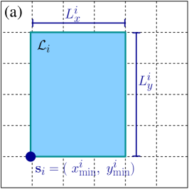
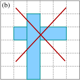
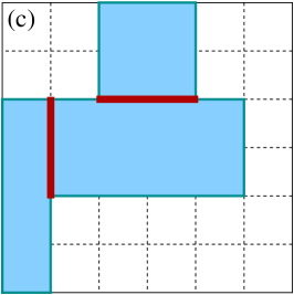
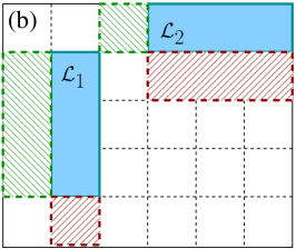
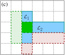
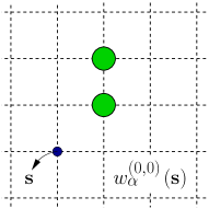
Consider a simple cubic lattice in dimensions where a lattice point is specified by a set of integers [Fig. 1(a)]. The lattice constant sets the unit of length. The particles of interest are rectangles in 2D and parallelepipeds in 3D. The state of a particle of species , denoted by , is fully determined by its position and its size vector . The size vector specifies the extent of the particle along each Cartesian direction. The position vector is given by the corner whose lattice coordinates are minimal each. The particles are assumed to have entropic interactions as well as energetic attractions. The entropic interaction prohibits overlapping of two or more particles [Fig. 1(b)]. A pairwise attraction can be expressed as a function of distance between particles of species and . We will consider effective attractions between particles induced by polymeric depletants of general type, but in actual numerical calculations we will only consider the limit of sticky rods where the attractive interaction between two particles is proportional to the number of their neighboring lattice sites [Fig. 1(c)].
II.2 Classical density functional theory
We will employ classical density functional theory (DFT) to investigate the system. In classical DFT, the grand potential functional for a -component mixture is a unique functional of the set of one-body density profiles where is the species index. Densities are computed as number of particles per lattice site. The equilibrium density profiles minimize the grand potential functional Eva79 ,
| (1) |
The grand potential functional is the Legendre transform of the total free energy of the system, i.e., the sum of the intrinsic free-energy functional and the interaction energy of each species with an external potential . For a lattice model the grand potential reads,
| (2) |
where is the chemical potential of species and the integrals appearing in the continuum become sums over discrete lattice positions . The intrinsic free-energy functional is further decomposed into an ideal gas contribution ,
| (3) |
and an excess (over ideal) part due to the interaction between the particles. Here, is the inverse temperature. For the following, we need to assume that we know an excess functional for a multicomponent system of hard particles. In the continuum, fundamental measure theory (FMT) provides such functionals (for a review see Ref. Rot10 ), and a lattice extension to multicomponent hard rods has been derived by Lafuente and Cuesta Laf02 ; Laf04 . In the framework of FMT, the excess free-energy density is expressed as a function of a set of weighted (smeared-out) densities . Each weighted density is computed as the sum over species of convolutions of a corresponding weight function and the density profile . For the lattice model, we assume can be expressed in the following FMT form:
| (4) |
where denotes the discrete convolution.
II.3 The AO model
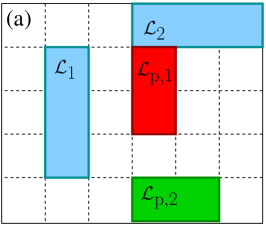
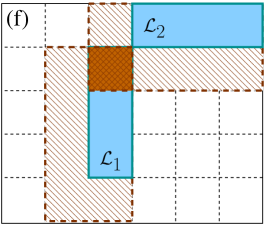
The short-ranged attractions between the lattice particles are induced by depletion interactions as in the AO model AO54 ; Vri76 . Consider non-adsorbing polymeric particles which do not have any mutual interaction, but a hard-core interaction with the particles in the system (we refer to the latter as colloidal particles). Due to the hard-core interaction of the polymeric and colloidal particles, there exists an excluded volume enclosing the colloidal particles which is composed of the proper volume of a colloidal particle itself together with a depletion layer and which the polymers are not allowed to enter. Note that polymeric particles occupying only one lattice site (i.e., with size in all lattice directions) do not induce an extra depletion layer. Hence a minimal polymeric particle inducing attractions is a rod with length in one direction and length 1 in the other directions. Such a polymer species will induce depletion attractions only along the direction where its length is 2. Hence one needs additional polymer rod species with length greater than one in the other lattice directions to induce corresponding depletion attractions. Due to our convention of specifying the position of a particle, the depletion layers are asymmetric in the lattice model (see Fig. 2). Overlap of the excluded volumes (corresponding to polymer species ) of two colloidal particles of species and increases the available free volume for them, hence their entropy. This results in an effective attraction between colloidal particles associated with polymer species . The induced effective attraction is proportional to the overlap volume of the corresponding excluded volumes, as well as to the osmotic pressure of polymer species . Assuming that the system is coupled to reservoirs of polymers which sustain the chemical potential of each polymer species in the system at a constant value , the osmotic pressure of each polymeric rods is equivalent to its corresponding reservoir polymer density . In summary,
| (5) |
One sees that the reservoir density is equivalent to an inverse temperature. Note that , and, consequently, the range of attraction, is determined by the size vector of polymer species (see Fig. 2). As the 2D example of Fig. 2 illustrates, for polymeric rods of length there is only a nonzero overlap of colloidal excluded volumes if the colloidal rods touch each other along the direction, and the overlap volume (overlap area in 2D) is given by the number of touching sites. Hence these rods induce sticky interactions along the direction [Fig. 2(c)]. Likewise, polymeric rods of length induce sticky interactions along the direction. Polymeric “squares” of length additionally introduce edge-edge attractions between the colloidal rods [Fig. 2(f)].
II.4 An FMT functional for short-ranged attractions
In order to construct an FMT functional for the AO model, consider a mixture of species of colloidal rods and species of non-adsorbing polymers whose density profiles are denoted by and , respectively. We start from the excess free-energy density of an -component mixture of hard rods (HR) . The polymeric rods are not interacting with each other, and therefore we will assume that for all combinations of polymer species and , their corresponding second-order direct correlation function vanishes. Since the direct correlation function is defined by
| (6) |
the terms in the excess free-energy density should be either constant or linear in polymer densities Schm00 . Hence the excess free-energy density of the AO model can be obtained by linearizing with respect to polymer densities . Since depends on the polymer densities only through the weighted densities , this results in the free-energy density
| (7) |
where and denote weighted densities for colloids and polymers, respectively. Likewise, and are weight functions for colloids of species and polymers of species . Note that the derivative has to be evaluated at zero polymer density, and thus it will depend only on . Equivalently, the excess free-energy density can be written as
| (8) |
where we have introduced , the first-order direct correlation function for polymer species defined as
| (9) | |||||
Here is a modified convolution operator. Therefore the total free-energy functional for the AO model can be written as follows:
| (10) | |||||
| (11) |
where the ideal gas part is given by Eq. (3) and the excess part by Eq. (8). Since we are dealing with a semi-grand ensemble, where the number of colloidal particles and the chemical potential of polymers is conserved, a more appropriate quantity for minimization is the semi-grand free energy which is the Legendre transformation of with respect to polymer densities:
| (12) |
For a given colloidal density profile , the equilibrium density of each polymer species is obtained by minimizing with respect to the corresponding polymer density.
| (13) |
where is the reservoir density of polymer species [see Eq. (5)] and is its corresponding first-order direct correlation function defined in Eq. (8). As a result, once the polymer reservoir densities are specified, the density profile of polymers is given by an explicit functional of only colloidal densities. When evaluated in the bulk (constant ), is equivalent to the relative part of the total volume available for polymer species (free volume fraction) Mor16 . Finally, it is desirable to obtain an effective free energy for colloidal particles which retains only the effect of the depletion interactions induced by the polymers. This is achieved by subtracting from those terms which are linear in the polymer densities and at most linear in the colloid densities Mor16 . These subtracted terms are equivalent to the grand potential of the polymers which interact at most with one colloidal particle and hence do not contribute to the effective attractions. Hence,
| (14) | |||||
where is the Mayor-f bond for the hard interaction between a colloidal rod of species at position and a polymer of species at position . The connection to the excluded volume for polymer species around a single colloidal particle of species (useful later) is given by
| (15) |
where and are respectively the th component of the size vectors of the colloid species and the polymer species .
The part in resulting from the depletion attractions is given by subtracting the ideal and excess free energy of the hard rods, . In the limit of small colloid densities it is given by
| (16) |
We call this the naive mean-field approximation. It sums over all two-particle depletion interactions induced by polymers. The depletion potential between a colloidal pair of particles belonging to species induced by polymer species is given by Eq. (5). Note that one can in principle work with negative reservoir densities such that the depletion potential becomes repulsive. For bulk systems (all colloidal densities are constant), Eq. (16) corresponds to the Bragg-Williams approximation.
Let us make a few remarks on the possible merits and limitations of the effective free-energy functional derived here. The effective AO functional contains multibody attractions if triple or higher overlaps of excluded volumes around colloidal particles are possible. Below, however, we will present results on rods with effectively pairwise sticky interactions to demonstrate the use of the AO model to treat short-ranged, pairwise interactions. The treatment of two-particle attractions is usually very difficult in DFT and therefore practical approximations often resort to a naive mean-field approximation of the type as in Eq. (16). (It works better than one might expect, see the discussion in Ref. Arch17 .) As is shown, the AO functional goes beyond it. The density expansion of the AO free energy [Eq. (12) or Eq. (14)] contains only terms up to linear order in , as a result of assuming vanishing direct correlation functions between the polymers. In the full AO model (with ideal polymers), the polymer-polymer direct correlation function does not vanish; its virial expansion starts with terms quadratic in the colloid density. Consequently, the density expansion of the full AO model contains higher-than-linear terms in (see Ref. San15 for a corresponding calculation of virial coefficients in the standard, continuum AO model). In Ref. BraderThesis it is extensively argued why the linearization of FMT-based functionals is still a good approximation. However, we expect deviations for high (equivalent to low temperatures). Further improvements in this direction might explore the ideas of Ref. Schmidt05 to treat the polymers as clusters in the construction of the functional. If an approximation for is used in deriving an explicit form for the AO functional, the low-density expansion of the effective attractive free energy will result in the correct form of Eq. (16) only if the functional expansion of in densities is correct up to third order.
In the following, as an exemplary case, we will use the method of Lafuente and Cuesta Laf02 ; Laf04 for constructing an FMT free-energy functional in the form of Eq. (4) for hard rods in the lattice model and the explicit derivation of an AO functional. The functional is applied to the case of sticky rods whose long axis is of length and all other axes are of length 1 for 2D and 3D systems, as well as a (2+1)D system, i.e., rods confined to a substrate. In this paper, we will discuss only the phase diagrams and leave considerations of inhomogeneous systems to later work. For this purpose, in each case an expression for the effective free-energy density is presented and the necessary equilibrium properties are obtained.
III FMT-AO from the Lafuente-Cuesta functional
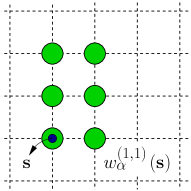
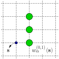
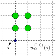
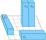
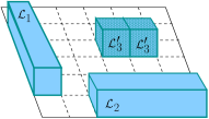
In Ref. Laf02 and Laf04 Lafuente and Cuesta have worked out an FMT excess free-energy density for hard bodies on a lattice model in the form of Eq. (4). For a given rod species , the specified weight functions and their corresponding weighted densities , are labeled by -dimensional index whose components are either 0 or 1. Each weight function can be interpreted as the support of a rod whose size vector is related to the size vector of the original rod species as follows
| (17) |
where is a -dimensional vector whose components are all 1. This means the side length of rod in dimension is identical to that of rod if the corresponding th component of is 1, while for we have , i.e., it is shortened by one lattice unit (see Fig. 3). In particular, for the size vectors of the support rod and the rod species are identical. The corresponding weighted density evaluated at lattice point returns the local packing fraction at that point.
The central physical insight that underlies this choice of weight functions and the subsequent construction of the functional is dimensional crossover. By applying an appropriate external potential to the particles of a -dimensional system, one can restrict the translational degrees of freedom of particles along a given axes and hence create a system in dimensions. An exact FMT functional should necessarily return the correct excess free energy of such a dimensionally reduced system. Of particular interest is the reduction to zero dimensions (0D) by confining the system to a 0D cavity which can hold exactly one particle. The excess free-energy density of a 0D cavity depending on its average occupation is exactly known and reads
| (18) |
Note that for an -component mixture one can define a set of 0D cavities with . The 0D cavity corresponding to species specifies a minimal set of points on the lattice which hold exactly one particle of species . The local packing fraction in the full (multi-species) cavity is evaluated as . Note that the excess free-energy density of all such 0D cavities is given by Eq. (18) with . Lafuente and Cuesta have derived a functional which returns the correct free energy for all possible 0D cavities in the system, i.e., it is correct for extreme confinement Laf02 ; Laf04 . The resulting Lafuente-Cuesta excess free-energy density is given by
| (19) |
where is the -dimensional index as before and is a difference operator which acts on a given function as: .
III.1 Two dimensions
For a -component mixture of hard rods with short axes of length 1 in 2D, consider species parallel to the axis and the remaining oriented along the axis. The corresponding excess free-energy density from Eq. (19) is given by
| (20) | |||||
where the fourth term vanishes since for the type of hard rods considered, and the other weighted densities are calculated as follows:
| (21) |
Here ’s are the density of species , are their corresponding weight functions, and denotes the discrete convolution defined in Eq. (4). Note that for [] the sum is restricted to those particles which lie along the axis [-axis] since only their corresponding weighted densities are not zero.
For the construction of an FMT-AO functional for attracting rods, we start from the excess free-energy density of a four-component mixture. We will consider two colloidal species whose size vectors are given by and . Moreover, we need two polymer species, and , for inducing the attractions. By setting equal polymer chemical potentials , and, consequently, equal polymer reservoir densities , we ensure a symmetric attractive interaction between colloidal particles along the and axes. The excess free-energy density for the AO model is obtained by linearizing from Eq. (20) with respect to polymer densities [see Eqs. (7)-(9)]. The required polymeric first-order direct correlation functions are given by
| (22) |
Hence, for a given polymer reservoir density and after specifying the colloidal density profiles, the equilibrium polymer densities is obtained using Eqs. (13) and (22). Consequently, the total free energy [Eq. (10)] and the semi-grand free energy [Eq. (12)] are obtained. Finally, the effective free energy for colloidal particles is fully determined as a functional of the colloidal densities by using Eq. (14) and the expressions for excluded volumes from Eq. (15).
In the following, we explicitly consider sticky attractions and discuss the results for a bulk state. Therefore, the polymer length which determines the range of attraction is set to . In a bulk (homogeneous) state and are constant. As a result, all colloidal weighted densities are constant, i.e., , where is the total colloidal density and is the packing fraction, , and . Consequently, the corresponding equilibrium polymer densities and polymeric weighted densities are also constant. Using Eqs. (13) and (22), the equilibrium polymer densities in bulk read
| (23) |
The total free-energy density of the system can be written as a sum of ideal gas free-energy density of colloidal and polymeric rods, and respectively, the entropic contribution to the excess free-energy density and the energetic contribution due to the attractive interactions:
| (24) | |||||
| (25) | |||||
| (26) | |||||
| (27) |
where the ideal gas free-energy density is defined in Eq. (3). Consequently, the semi-grand free-energy density and the effective colloidal free-energy density read
| (28) | |||||
The attractive part of the effective free-energy density is linear in and the leading term for small colloidal rod densities is quadratic in these and equivalent to the Bragg-Williams approximation since the virial expansion of the LC functional is correct up to third order. The Bragg-Williams approximation of the attractive part gives a term . The case corresponds to the lattice gas. Setting and [we have only one component for particles with extension (1,1)], the effective free-energy density reduces to the Bragg-Williams approximation for all densities:
| (30) |
For the determination of the bulk phase diagram it is useful to introduce an order parameter for demixing:
| (31) |
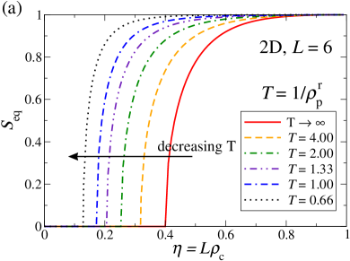
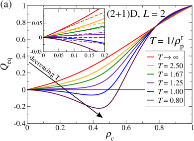
For and for a given total colloidal density , the equilibrium value for the demixing order parameter minimizes the effective free-energy density. For small densities, the mixed state has the minimum free energy, i.e., . On increasing , we reach a critical density above which we have a demixed state. For a pure hard-rod system, it has been shown that for the system demixes at Oet16 . Taking the attractive interactions into account, this transition shifts to lower densities for a given colloidal rod length . This is shown in Fig. 4(a) for rod length .
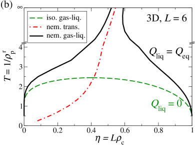
The complete phase diagram for a fixed rod length [ in Fig. 4(b)] reflects the competition between demixing (present for all ) and the gas-liquid transition (setting in above a critical ). The gas-liquid binodal for a coexisting isotropic gas state and an assumed isotropic liquid state is shown by the green dashed line in Fig. 4(b). However, the coexisting isotropic liquid state is unstable since the liquid branch is above the critical density of demixing [red dot-dashed line in Fig. 4(b)]. Therefore the gas-liquid binodal [full black line in Fig. 4(b)] becomes deformed: The demixing line, starting from the hard-rod limit () ends in a tricritical point below which coexistence between an isotropic gas state and a demixed liquid state is found.
The FMT-AO free-energy density delivers the phase behavior of the competing demixed and gas-liquid phases from a single expression for the free-energy density. This goes beyond existing theoretical treatments such as in Ref. Lon12 which have to resort to different free energy models for an isotropic and a fully demixed state. However, a comparison to available simulation results shows the well-known difficulties of mean-field models in 2D. In Ref. Lon10 , the system is studied by a mixture of canonical and grand-canonical Monte Carlo methods. It is found that also in the case of attractions demixing is only present for (as for hard rods). Demixing shifts to higher rod densities with increasing attractions, in contrast to our theory results here and the results in Ref. Lon12 . This appears surprising since one might think that the sticky attractions increase the propensity of the rods to align and thus favor the demixed phase (with alignment). Control simulations performed by us suggest that the sticky rods organize in larger domains of locally aligned rods with no alignment globally. These domains fluctuate strongly in size and shape, and the entropic contribution of such fluctuations is not captured by the theoretical treatments. Furthermore the simulations of Ref. Lon10 suggest that the critical point of the gas-(isotropic) liquid transition survives with increasing attractions. From the simulation results it is not clear whether the demixing line meets the liquid branch of the gas-liquid binodal in a tricritical point or in a critical end point.
III.2 Three dimensions
Consider a -component mixture of hard rods with short axes of length 1 in 3D, of which species are oriented parallel to the axis, species are oriented parallel to the axis, and the remaining species are oriented parallel to the axis. The excess free-energy density from Eq. (19) is in this case
| (32) | |||||
Note that all other weighted densities with are zero. The non-vanishing weighted densities are calculated as follows:
| (33) |
where, as in Eq. (21), the sums in the last three weighted densities are restricted to the species which are extended along the axis where the corresponding index is zero.
For the construction of an FMT-AO functional for attracting 3D rods, consider three species of colloidal hard rods with equal length and size vectors , , and . For inducing attractions along each axis, we need three polymer species with size vectors , , and . As in the derivation of the 2D functional, we assume that the corresponding polymer reservoir densities have the same value . Hence, we have to start from the excess free-energy density of a six-component hard-rod mixture in 3D, i.e., Eq. (32) with the weighted densities from Eq. (33). Linearization with respect to the polymer densities results in the following polymeric first-order direct correlation functions:
| (34) |
Consequently, for a given and colloidal rod densities , the equilibrium polymer densities , the total free energy , the semi-grand free energy , and, finally, the effective free energy for colloidal rods only are determined by Eqs. (10)-(15).
Now we turn to a bulk state where all colloidal densities are constant. The non-vanishing colloidal weighted densities are given by with the total colloidal density and the packing fraction, , , and . As in 2D, we will only consider sticky attractions, i.e., . Using Eqs. (13) and (34), the equilibrium polymer densities in bulk become
| (35) |
Similar steps as in the 2D case lead to the following effective free-energy density:
| (36) |
with
| (37) | |||||
As before, for small the attractive part is quadratic in the colloidal rod densities and will reduce to the correct form of the Bragg-Williams approximation.
The phase diagram determination is facilitated by the introduction of two order parameters, usually denoted as the nematic order parameter and the biaxiality parameter :
| (38) |
and in terms of these the density of each colloidal species is determined as
| (39) |
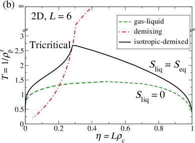
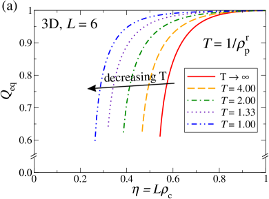
For a given colloidal density , the equilibrium value of the order parameters, and , is obtained by a simultaneous minimization of the effective free-energy density. It turns out that for a given polymer reservoir density, for all densities. However, the nematic order parameter shows a first-order transition from an isotropic state to a nematic state with . For hard rods, the transition is present for and the associated critical packing fraction shifts to lower packing fractions for longer rods Oet16 . Coexisting isotropic and nematic states are separated by a substantial density gap. On switching on the attractions, we find, generally, that the critical packing fraction decreases on increasing and that the density gap between coexisting isotropic and nematic states continuously widens (for and ). We illustrate this for in Fig. 5. Figure 5(a) shows the behavior of for different effective temperatures which displays the discontinuous jump as well as the shift of the critical packing fraction to lower values on decreasing . Figure 5(b) shows the corresponding phase diagram. As in the 2D case, we have calculated the binodal for an isotropic gas-liquid transition (, green dashed line). The line of critical packing fractions is shown by the red dot-dashed line and one sees that the liquid branch of the isotropic gas-liquid binodal is unstable with respect to the onset of nematic order. Therefore the physical binodal (full black line) corresponds to coexistence between an isotropic, lower density state and a nematic, higher-density state for all . The density gap is continuously increasing with decreasing and thus the isotropic-nematic transition smoothly acquires the character of a gas-liquid transition as well.
Simulation results for 3D lattice rods with attractions are not available, whereas for rods in the continuum there are Bol97 . For continuum rods at higher densities, there is a transition from the nematic phase to a smectic and a crystalline phase. On increasing attractions, the isotropic-nematic transition becomes unstable in favor of the more ordered smectic and crystalline phases. Therefore one observes a similar widening of the coexistence gap on increasing the attractions as in the lattice model but the coexisting states correspond to an isotropic gas state and either a solid state (when polymers induce the attractions) or a smectic state (when there is an explicit pairwise, attractive potential between the rods) Bol97 .
III.3 Monolayer ((2+1)D)
Here we consider a monolayer of rods on a substrate which can lie down or stand up. It can serve as a toy model for Langmuir monolayers or a thin film of anisotropic organic molecules as often investigated in the context of research on organic semiconductors review-OMBD-Schreiber ; review-OMBD-Witte-Woell . Effectively, the system can be mapped onto a mixture of species in 2D. The species of standing-up rods are treated as their projection on the substrate, i.e. particles with size vector . The remaining species are defined as in the 2D system. The corresponding excess free-energy density is the same as in Eq. (20) with the weighted densities provided by Eq. (21). Note that in calculating the corresponding weighted density of “standing-up” rods, , are also considered.
For constructing an FMT-AO functional for sticky rods in (2+1)D, consider three species of colloidal rods, with size vectors denoted by and for lying-down rods and for standing-up rods. By adding two polymer species, and and with reservoir density each, the in-plane attractive interactions are ensured. However, the out-of-plane interactions of two neighboring standing-up rods is underestimated by a factor of (see Fig. 6). In order to compensate this, we will add two more polymer species and which only interact with the standing-up rods and have an enhanced polymer reservoir density . As a result, we are dealing with the excess free-energy density of a 2D hard-rod mixture [Eq. (20)], with seven components: three colloidal and four polymeric species. Moreover, in linearization of with respect to polymer densities, there is a slight difference to the 2D case: the additional polymer species, and , are not interacting with in-plane colloidal rods, and . As a result, in calculation of corresponding ’s, the density of and should be set to zero as well. and are determined similar to those of 2D case. The polymeric first-order direct correlation functions in this (2+1)D system are given as follows:
| (40) |
After fixing , the equilibrium density of polymer species are determined by Eq. (13) with from Eq. (40). Consequently, the total free energy and the semi-grand free energy are determined from Eqs. (10) and (12). Finally by using Eqs. (14) and (15) we obtain an effective free energy for colloidal particles for a (2+1)D system.
For a bulk state, the density of colloidal rods and consequently their corresponding weighted densities are constant, , , and . For sticky attractions , the equilibrium density of polymeric rods is obtained by combining Eqs. (13) and (40).
| (41) |
Similar steps as in the two cases before lead to the following effective free-energy density:
| (42) | |||||
with
| (43) | |||||
Here the attractions between only the standing rods is equivalent to the Bragg-Williams approximation, whereas for all other attractions corrections to the Bragg-Williams approximation are present for higher colloidal densities.
The determination of phase diagrams proceeds via the introduction of order parameters as in the 3D case [see Eqs. (38) and (39)]. Equilibrium value of the demixing and the nematic order parameters are obtained by minimizing the effective free-energy density with respect to corresponding order parameters. This implies that for a given rod length and temperature , the corresponding chemical potentials and should be zero.
For a pure hard-rod system and in the regime of small rods , for all densities and a continuous transition from an isotropic state at to a nematic state for a fully packed system is observed. For larger rods a reentrant demixing occurs for a certain interval Oet16 . With attractions, such a reentrant behavior persists and occurs also for lower , which is understandable since for an attractive system in 2D and for a given rod length , the demixing transition density shifts to lower values on decreasing the effective temperature (see Fig. 4). Hence, for a monolayer one expects to find a certain temperature below which the planar rods are demixed for . Since the rods eventually stand up with increasing total density, there exists a higher density at which the lying rods mix again and . In order to calculate and , we start from obtaining by setting . Expanding ,
| (44) |
the de- and remixing densities are obtained numerically by computing the densities at which . In general, we find that for moderate attractions demixing is relevant for and that the phase diagram becomes very complicated due to the competition of upright (nematic) ordering, demixing in the plane and the gas-liquid transition. However, the comparison to available simulation results in 2D has shown that FMT-AO overestimates the tendency to demix in the substrate plane. Therefore we focus on shorter rods ( and 3) for the calculation of equilibrium order and phase transitions.
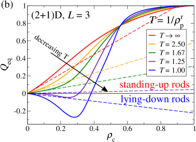
The equilibrium value of the nematic ordering parameter for and is shown in Fig. 7(a) and 7(b). Nematic order, i.e., , sets in already at . In order to obtain the low-density behavior, we expand (assuming ):
| (45) | |||||
The equilibrium nematic order parameter is obtained by setting , and in leading order in it is given by
| (46) |
The nematic order parameter is linear in the total rod density [shown by the dashed lines in Fig. 7(a) and 7(b)]. Starting from a pure hard-rod system () for a given rod length, the tendency to order upright becomes weaker as the temperature is decreased. Eventually, one reaches a certain temperature below which and the rods preferably order in-plane for small densities.
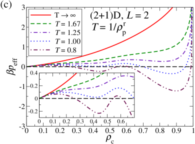
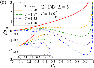
In Fig. 7(c) and 7(d) we show results for the pressure for and 3, respectively. For effective temperatures below an upper critical temperature, , the van der Waals loop points to a stable phase coexistence between a low-ordered state at a smaller density and an upright-ordered state at a larger density. By further decreasing the temperature, a secondary loop is observed whose interpretation will be different for and . The associated phase diagrams for and 3 are shown in Fig. 8 which are shown in the plane with axes total colloidal density and effective temperature . For [Fig. 8(b)] the upper critical temperature is at and the binodal for the coexisting states (low density and low order vs. higher density and upright order) is stable for all temperatures (full black line). For [Fig. 8(a)] the upper critical temperature is at and the corresponding binodal is shown by the red dashed line. Below a second, lower critical temperature a second stable binodal appears (blue dashed line) which marks coexistence between two low-ordered states. This second binodal is actually akin to the gas-liquid transition between isotropic states which we have computed by setting (green dotted line) and which is very close to the second binodal. Both the first and second binodals become unstable below a triple temperature and give way to a binodal marking the coexistence between a nearly isotropic gas and a highly ordered liquid at high densities (full black line). For [Fig. 8(b)] the second binodal is inside the first one () and thus metastable (purple dot-dot-dashed line). Again, it is almost on top of the gas-liquid binodal for isotropic states (green dotted line). For , there are two more features in the phase diagram. The red dashed line shows the region of reentrant demixing in the substrate plane which occurs at low temperatures . The black dash-dash-dotted line corresponds to a discontinuous jump in the nematic order parameter which sets in at a third critical temperature and which would give rise to a first-order nematic-nematic transition. Both transitions (reentrant demixing and nematic-nematic) are metastable for but would become stable for higher according to FMT-AO.
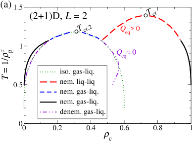
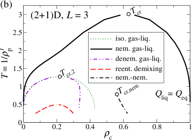
These results suggest that the phase diagrams of monolayers can be extremely rich. Previous studies have identified the transition between a nearly isotropic gas state and a high density, upright-ordered state Boehm77 ; Kra92 , corresponding to the full black line in Fig. 8(b). This should be the stable transition for intermediate (Ref. Kra92 confirms this also by performing Monte Carlo simulations for ). We emphasize that this is not the “descendant” of the gas-liquid transition between isotropic states but rather a new nematic liquid-liquid transition. It would be very interesting to check with simulations whether the two critical points associated with this “new” nematic liquid-liquid transition and the “old” gas-liquid transition are stable for , as we have found here. Such investigations should also be extended to monolayers in the continuum with short rods. We have not explored a possible substrate potential as an additional degree of freedom which in our opinion may shift the onset of metastability for the various transitions quite substantially.
IV Summary and outlook
In this work, we have derived a density functional for a lattice model with attractive anisotropic particles (rods). The attractions are induced by lattice polymers which interact hard with the rods and are an ideal gas amongst themselves (Asakura-Oosawa model). The functional is derived from a multi-component hard rod functional (for rods and polymers) via linearization with respect to the polymeric components. Explicit functionals are obtained by using the Lafuente-Cuesta functional Laf02 ; Laf04 for the multi-component hard rod system. We have applied the functional to the calculation of phase diagrams for sticky rods of length in 2D, 3D, and in a monolayer system [(2+1)D]. In all cases, there is a competition between ordering and gas-liquid transitions. In 2D, this gives rise to a tricritical point, whereas in 3D, the isotropic-nematic transition crosses over smoothly to a gas-nematic liquid transition. The richest phase behavior is found for the monolayer system on a neutral substrate. For , we find two stable critical points corresponding to the isotropic gas-liquid transition and a nematic liquid-liquid transition. For , the isotropic gas-liquid transition becomes metastable. There are further metastable transitions such as reentrant demixing in the substrate plane and a nematic-nematic first-order transition. These become stable for larger but we have not investigated this in detail.
In this work we have not exploited yet the capabilities of our explicit functional in investigating inhomogeneous situations (correlation functions, interfaces between coexisting states, or wetting/surface transitions on substrates). This will be done in future work. Of particular interest is also the description of film growth on substrate via a suitable lattice dynamic density functional theory. First steps in this direction have been taken by calculating the growth of a hard rod monolayer Klo17 which shows satisfactory agreement between dynamic DFT and kinetic Monte Carlo simulations. The extension of these investigations to attractive rods is desired to connect better to actual experimental systems.
Acknowledgment: This work is supported within the DFG/FNR INTER project “Anisotropic Thin Film Growth” by the Deutsche Forschungsgemeinschaft (DFG), Project No. OE 285/3-1.
References
- (1) K. Huang, Statistical Mechanics (Wiley, New York, 1987), Chap. 14.
- (2) V. R. Dugyala, S. V. Daware, and M. G. Basavaraj Soft Matter 9, 6711 (2013).
- (3) S. Sacanna and D. J. Pine, Current Opinion in Colloid and Interface Science 16, 96 (2011).
- (4) E. A. DiMarzio, J. Chem. Phys. 35, 658 (1961).
- (5) R. Alben, Mol. Cryst. and Liq. Cryst. 13, 193 (1971).
- (6) M. Oettel, M. Klopotek, M. Dixit, E. Empting, T. Schilling, and H. Hansen–Goos, J. Chem. Phys. 145, 074902 (2016).
- (7) M. A. Cotter and D. E. Martire, Mol. Cryst. and Liq. Cryst. 7, 295 (1969).
- (8) D. Dhar, R. Rajesh, and J. F. Stilck, Phys. Rev. E 84, 011140 (2011).
- (9) A. Ghosh and D. Dhar, Europhys. Lett. 78, 20003 (2007).
- (10) A. Gschwind, M. Klopotek, Y. Ai, and M. Oettel, Phys. Rev. E 96, 20003 (2017).
- (11) N. Vigneshwar, D. Dhar, and R. Rajesh, Different phases of a system of hard rods on three dimensional cubic lattice, arXiv:1705.10531.
- (12) T. L. Hill, An Introduction to Statistical Thermodynamics (Addison-Wesley, Reading, MA, 1960), Chap. 14.
- (13) P. Longone, M. Davila, and A. J. Ramirez-Pastor, Phys. Rev. E 85, 011136 (2012).
- (14) P. Longone, D. H. Linares, and A. J. Ramirez-Pastor, J. Chem. Phys. 132, 184701 (2010).
- (15) R. E. Boehm and D. E. Martire, J. Chem. Phys. 67, 1061 (1977).
- (16) D. Kramer, A. Ben-Shaul, Z.-Y. Chen, and W. M. Gelbart, J. Chem. Phys. 96, 2236 (1992).
- (17) S. Asakura and F. Oosawa, J. Chem. Phys. 22, 1255 (1954) and J. Polym. Sci. 33, 183 (1958).
- (18) A. Vrij, Pure Appl. Chem. 48, 471 (1976).
- (19) M. Schmidt, H. Löwen, J. M. Brader, and R. Evans, Phys. Rev. Lett. 85, 1934 (2000).
- (20) J. M. Brader, R. Evans, and M. Schmidt, Mol. Phys. 101, 3349 (2003).
- (21) L. Lafuente and J. A. Cuesta, J. Phys.: Condens. Matter 14, 12079 (2002).
- (22) L. Lafuente and J. A. Cuesta, Phys. Rev. Lett. 93, 130603 (2004).
- (23) M. Mortazavifar and M. Oettel, J. Phys.: Condens. Matter 28, 244018 (2016).
- (24) R. Evans, Advances in Physics 28, 143 (1979).
- (25) R. Roth, J. Phys.: Condens. Matter 22, 063102 (2010).
- (26) A. J. Archer, B. Chacko, and R. Evans, J. Chem. Phys. 147, 034501 (2017).
- (27) A. Santos, M. Lopez de Haro, G. Fiumara, and F. Saija, J. Chem. Phys 142, 224903 (2015).
- (28) J. M. Brader, Statistical Mechanics of a Model Colloid-Polymer Mixture, Ph.D dissertation, H. H. Wills Physics Laboratory, University of Bristol (2001), http://www.bristol.ac.uk/physics/media/theory-theses/brader-jm-thesis.pdf.
- (29) J. A. Cuesta, L. Lafuente, and M. Schmidt, Phys. Rev. E 72, 031405 (2005).
- (30) P. G. Bolhuis, A. Stroobants, D. Frenkel, and H. N. W. Lekkerkerker, J. Chem. Phys. 107, 1551 (1997).
- (31) F. Schreiber, Phys. Stat. Sol. A 201, 1037 (2004).
- (32) G. Witte and C. Wöll, J. Materials Res. 19, 1889 (2004).
- (33) M. Klopotek, H. Hansen-Goos, M. Dixit, T. Schilling, F. Schreiber, and M. Oettel, J. Chem. Phys 146, 084903 (2017).