Observing pure effects of counter-rotating terms without ultrastrong coupling:
A single photon can simultaneously excite two qubits

Abstract

The coherent process that a single photon simultaneously excites two qubits has recently been theoretically predicted by [Phys. Rev. Lett. 117, 043601 (2016)]. We propose a different approach to observe a similar dynamical process based on a superconducting quantum circuit, where two coupled flux qubits longitudinally interact with the same resonator. We show that this simultaneous excitation of two qubits (assuming that the sum of their transition frequencies is close to the cavity frequency) is related to the counter-rotating terms in the dipole-dipole coupling between two qubits, and the standard rotating-wave approximation is not valid here. By numerically simulating the adiabatic Landau-Zener transition and Rabi-oscillation effects, we clearly verify that the energy of a single photon can excite two qubits via higher-order transitions induced by the longitudinal couplings and the counter-rotating terms. Compared with previous studies, the coherent dynamics in our system only involves one intermediate state and, thus, exhibits a much faster rate. We also find transition paths which can interfere. Finally, by discussing how to control the two longitudinal-coupling strengths, we find a method to observe both constructive and destructive interference phenomena in our system.

I Introduction

The light-matter interaction between a quantized electromagnetic field and two-level atoms has been the central topic of quantum optics for half a century, and has developed into the standard cavity quantum electrodynamics (QED) theory. In a QED system, if the dipole-field or dipole-dipole coupling strengths ($\lambda$) are weak compared with the cavity or atomic transition frequencies ($\omega_{c}$ and $\omega_{q}$, respectively), we often routinely adopt the rotating-wave approximation (RWA). Under the RWA, one can neglect the excitation-number-nonconserving terms Bloch and Siegert (1940); Jaynes and Cummings (1963); Shore and Knight (1993); Irish (2007), which, compared with the resonant terms, are usually only rapidly oscillating virtual processes and negligibly contribute to the dynamical evolution of such a system Scully and Zubairy (1997).

In fact, the RWA works well even in the strong-coupling regime. Only in the ultrastrong and deep-strong coupling regimes [where $\lambda>0.1\times\min{(\omega_{c},\omega_{q})}$ and $\lambda>\min{(\omega_{c},\omega_{q})}$, respectively] Anappara et al. (2009); Forn-Díaz et al. (2010); Niemczyk et al. (2010); Forn-Díaz et al. (2010); Geiser et al. (2012); Scalari et al. (2012); Baust et al. (2016); Forn-Díaz et al. (2017); Yoshihara et al. (2017); Chen et al. (2017), the counter-rotating terms have apparent effects in a QED system Braak (2011); Gu et al. (2017). The excitation-number-nonconserving terms in a QED system can lead to many interesting quantum effects Niemczyk et al. (2010); Ashhab and Nori (2010); Cao et al. (2010, 2011, 2012); Casanova et al. (2010); Garziano et al. (2015); Wang et al. (2016a), such as three-photon resonances Ma and Law (2015), the modification of the standard input-output relation Ridolfo et al. (2012, 2013), quantum phase transitions Hwang et al. (2015), frequency conversion Kockum et al. (2017a), or the deterioration of photon blockade effects Hwang et al. (2016); Le Boité et al. (2016). However, all of these phenomena are the combined and mixed effects of both counter-rotating and resonant terms. Here we address, in particular, the following questions: How can we observe some pure effects of counter-rotating wave terms in a QED system, i.e., without being disturbed by the resonant terms? Moreover, is it really always reasonable to apply the RWA in dipole-field or dipole-dipole coupling systems, which are far way from the ultrastrong-coupling regime?

Other interesting quantum processes are multi-excitation and emission in a QED system. The process that a two-level atom (molecule) absorbs two or more photons simultaneously has been widely discussed in many quantum platforms Denk et al. (1990); So et al. (2000); Garziano et al. (2015); Wang et al. (2016a); Chen et al. (2017). However, the inverse process (of a single photon splitting to excite two and more atoms) is rarely studied Garziano et al. (2016); Kockum et al. (2017b); Stassi et al. (2017).

Recently, Garziano et al. Garziano et al. (2016) predicted that one photon can simultaneously excite two or more qubits. In their theoretical proposal, two superconducting qubits are coupled to a resonator with both longitudinal and transverse forms in the ultrastrong-coupling regime. A similar process was predicted via the photon-mediated Raman interactions between two three-level atoms (qutrits) in the strong-coupling regime Zhao et al. (2017). Note that both dynamics (with qubits Garziano et al. (2016) and qutrits Zhao et al. (2017)) were composed of three virtual processes, which do not conserve the number of excitations. Also the effective transition between atoms and a single photon is of a relatively slow rate.

In this paper, we propose a superconducting system composed of a transmission-line resonator longitudinally coupled with two flux qubits. The two qubits couple to each other via an antiferromagnetic dipole-dipole interaction. We show that, when the sum of two qubits transition frequencies is approximately equal to the resonator frequency, the counter-rotating terms in the dipole-dipole interaction cannot be dropped even when the system has not entered into the ultrastrong-coupling regime. The RWA is not valid here; on the contrary, the resonant terms can be approximately neglected in our model. Due to the counter-rotating terms, a single photon in the resonator can simultaneously excite two qubits. Finally, we discuss the quantum interference effects between four transition paths. Compared with the similar dynamics studied in Refs. Garziano et al. (2016); Zhao et al. (2017), the whole transition process proposed now only involves a single intermediate step, and the process rate can be much faster. Additionally, our proposal does not require to induce both longitudinal and transverse couplings Garziano et al. (2016), so the superconducting qubit can work at the optimal point and, thus, the pure-dephasing rate of the qubits can be effectively suppressed Fedorov et al. (2010); Stern et al. (2014); Garziano et al. (2015); Wang et al. (2016a). Moreover, we consider qubits instead of the qutrits studied in Ref. Zhao et al. (2017). By discussing the parameters in our system, we find that the coherence rate can easily exceed the decoherence rate, and it is possible to observe these quantum effects with current experimental setups.

Superconducting circuits with Josephson qubits are a suitable platform to explore our proposal as will be discussed in detail in Sec. II. We note that the past few years have witnessed the rapid development in quantum control and quantum engineering based on superconducting quantum circuits Gu et al. (2017); Makhlin et al. (2001); You and Nori (2005); Liu et al. (2005a); Clarke and Wilhelm (2008); DiCarlo et al. (2010); You and Nori (2011); Buluta et al. (2011); Xiang et al. (2013); Georgescu et al. (2014). The current manufacturing, control, and detection technologies for the superconducting devices are mature van der Wal et al. (2000); Liu et al. (2005b); Neeley et al. (2008); Chen et al. (2011); Inomata et al. (2016). Many quantum phenomena in atomic physics and quantum optics, such as vacuum Rabi oscillations Gu et al. (2017), Autler-Townes splitting Sillanpää et al. (2009); Wang et al. (2016b); Gu et al. (2016), and Fock states generation Hofheinz et al. (2008, 2009); Premaratne et al. (2017), have been demonstrated based on superconducting quantum circuits Gu et al. (2017). Moreover, since the dipole moments of a superconducting qubit are extremely large compared with the ones in natural atoms, the coupling strength in a circuit QED system Blais et al. (2004); Xiang et al. (2013), can enter into the strong, ultrastrong Niemczyk et al. (2010); Forn-Díaz et al. (2010); Baust et al. (2016); Forn-Díaz et al. (2017); Chen et al. (2017), and even deep-strong Yoshihara et al. (2017) regimes. All these advantages make superconducting quantum circuits an ideal platform for exploring various quantum effects beyond the RWA.

II Model

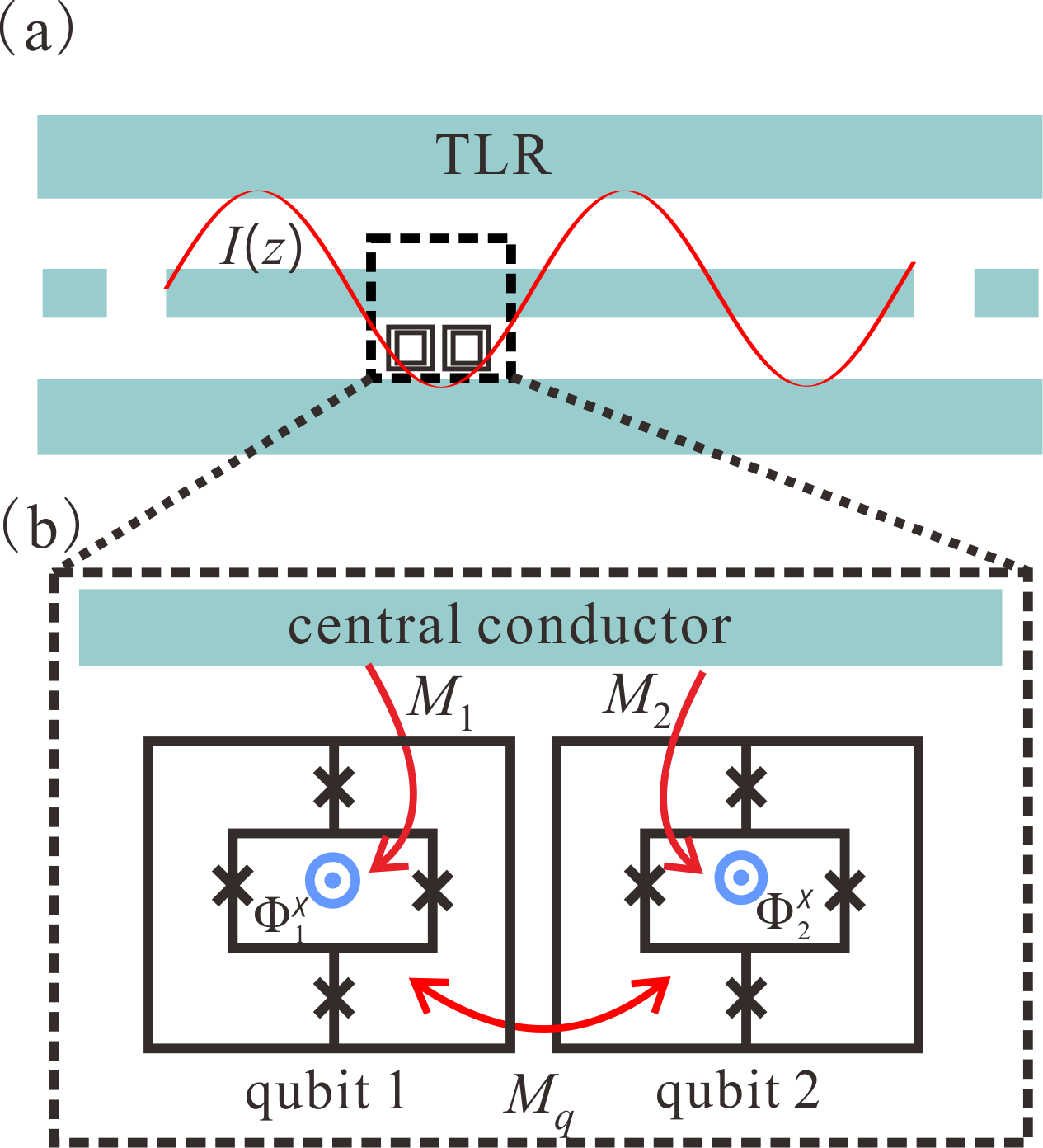
Figure 1: (Color online) (a) Schematic circuit layout of our proposal. The central conductor of the transmission-line resonator (TLR) is stretched in the $z$ direction, and the two flux qubits are placed at the antinode positions of the TLR standing-wave current $I(z)$. Here we assume that each qubit is composed of two symmetric gradiometric loops and a SQUID loop. (b) The quantized current $I(z)$ through the TLR central conductor can interact with the first and second qubit SQUID loops via mutual inductances $M_{1}$ and $M_{2}$, respectively. Each qubit is composed of four Josephson junctions (modeled by black crosses). To bias the energy gap of each qubit, a static flux $\Phi_{j}^{x}$ must be through the $j$th SQUID loop. The two qubits couple together with their mutual inductance $M_{q}$.

Our model can be implemented in a superconducting quantum circuit layout with Josephson junctions. As shown in Fig. 1, we consider two gap-tunable flux qubits Mooij et al. (1999); Orlando et al. (1999); You et al. (2007); Paauw et al. (2009); Fedorov et al. (2010); Stern et al. (2014) placed in a transmission-line resonator (TLR), and coupled together with an antiferromagnetic interaction Niskanen et al. (2006); et al. (2006); Harris et al. (2009). The Hamiltonian for the two qubits is expressed as (setting $\hbar=1$):

$$\bar{H}_{q}=\frac{1}{2}\sum_{j=1}^{2}(\Delta_{j}\bar{\sigma}_{j}^{x}+\epsilon_{j}\bar{\sigma}_{j}^{z})+J\bar{\sigma}_{1}^{z}\bar{\sigma}_{2}^{z},$$ (1)

where the energy basis $\epsilon_{j}=2I_{p,j}(\Phi_{j}^{z}-\Phi_{0}/2)$ can be controlled via the flux $\Phi_{j}^{z}$ through the two symmetric gradiometric loops Paauw et al. (2009); Stern et al. (2014), $\Delta_{j}$ is the energy gap, $\Phi_{0}$ is the flux quantum, and $\bar{\sigma}_{z}^{j}$ and $\bar{\sigma}_{x}^{j}$ are the Pauli operators for the $j$th qubit in the basis of persistent current states: $|\uparrow_{j}\rangle$ (counterclockwise) and $|\downarrow_{j}\rangle$ (clockwise) with amplitude $I_{p,j}$ Mooij et al. (1999); Orlando et al. (1999). The dipole-dipole interaction strength $J$ is given by $J=M_{q}I_{p,1}I_{p,2}$, where $M_{q}$ is the mutual inductance between two qubits Niskanen et al. (2006); et al. (2006); Harris et al. (2009). For such a layout arrangement, the mutual inductance $M_{q}$ and coupling strength $J$ are determined by the geometry and spatial relation, when the qubits are placed next to each other. Alternatively, as discussed in Refs. Averin and Bruder (2003); Wallquist et al. (2005); Harris et al. (2007); Tsomokos et al. (2010), one can achieve a tunable indirect coupling by employing a coupler, which allows a flexible coupling between two distant qubits. Here we just assume the two flux qubits as an example, and they can be replaced by some other type of superconducting artificial qubits (see, e.g., Figs. 1 and 2 in Ref. Gu et al. (2017)).

The energy gap $\Delta_{j}$ can be controlled conveniently by adjusting the static flux $\Phi_{j}^{x}$ through the SQUID loop. Since the sizes of two qubits ($\sim 10~{}\mu$m) are negligible compared with the TLR wave-length ($\sim$ cm), we assume that the resonator current is independent of the resonator position, and the dipole approximation is valid here. The qubits are placed at the antinode position $z_{0}$ of the TLR current Blais et al. (2004); Xiang et al. (2013); Gu et al. (2017). Since each qubit has two symmetric gradiometric loops, the flux contribution from the current $I(z)$ in the central conductor of the TLR vanishes to the first order of the energy bias $\epsilon_{j}$ Paauw et al. (2009); Fedorov et al. (2010); Stern et al. (2014). However, the current $I(z)$ in the central conductor of the TLR can produce flux perturbations to the SQUID loop of the $j$th qubit via the mutual inductance $M_{j}$ Paauw et al. (2009); Fedorov et al. (2010). Therefore, $\Delta_{j}$ can be expressed as

$$\Delta_{j}=\Delta_{j}(\Phi_{j0}^{x})+R_{j}M_{j}I(z_{0}),$$ (2)

where $R_{j}=\partial\Delta_{j}(\Phi_{j}^{x})/\partial\Phi_{j}^{x}$ is the sensitivity of the energy gap $\Delta_{j}$ on the static-flux frustration at the position $\Phi_{j0}^{x}$ Paauw et al. (2009); Fedorov et al. (2010). The quantized current of the TLR can be directly obtained from the quantization of the voltage and expressed as Yurke and Denker (1984); Blais et al. (2004); Gu et al. (2017); Clerk et al. (2010):

$$I(z_{0})=\sqrt{\frac{\omega}{2L_{0}L}}(a+a^{{\dagger}}),$$ (3)

where $L_{0}$ is the inductance per unit length of the TLR, $a$ ($a^{{\dagger}}$) denotes the annihilation (creation) operator of a microwave photon in the TLR, $\omega$ is the resonant mode frequency considered here, and $L$ is the total length of the resonator Yurke and Denker (1984); Blais et al. (2004). The coupling strength between the $j$th qubit and a single microwave photon in the resonator has the form

$$g_{j}=R_{j}M_{j}\sqrt{\frac{\omega}{2L_{0}L}},$$ (4)

and the total Hamiltonian for the whole system can be written as

$$\bar{H}_{T} = \omega a^{{\dagger}}a+\frac{1}{2}\sum_{j=1}^{2}(\Delta_{j}\bar{\sigma}_{j}^{x}+\epsilon_{j}\bar{\sigma}_{j}^{z})$$ (5)

$$+\sum_{j=1}^{2}g_{j}\bar{\sigma}_{j}^{x}(a+a^{{\dagger}})+J\bar{\sigma}_{1}^{z}\bar{\sigma}_{2}^{z}.$$

In an experiment, if we apply static fluxes $\Phi_{1}^{x}$ and $\Phi_{2}^{x}$ through the SQUID loop of two qubits with the opposite (same) direction, the flux sensitivities of the energy gaps $R_{1}$ and $R_{2}$ are of the opposite (same) sign. Moreover, by setting the $j$th qubit working at different energy-gap points $\Delta_{j}$, the amplitude of $R_{1}$ and $R_{2}$ can be easily modified Paauw et al. (2009); Fedorov et al. (2010). It can be found that $R_{1}$ and $R_{2}$ can directly determine the strengths and relative sign between $g_{1}$ and $g_{2}$. The coupling strengths between the qubits and resonator can be conveniently adjusted in this circuit QED system according to Eq. (4). In Sec. IV, we demonstrate how to obtain different interference effects by modifying $R_{1}$ and $R_{2}$.

To minimize the pure dephasing effect of two qubits induced by the flux noise, we often operate the qubits at their optimal points with $\epsilon_{j}=2I_{p,j}(\Phi_{j}^{z}-\Phi_{0}/2)=0$, by applying a static flux $\Phi_{j}^{z}=\Phi_{0}/2$ Paauw et al. (2009); Stern et al. (2014) through two gradiometric loops. In the new basis of the eigenstates $|e_{j}\rangle=(|\uparrow_{j}\rangle+|\downarrow_{j}\rangle)\sqrt{2}$ and $|g_{j}\rangle=(|\uparrow_{j}\rangle-|\downarrow_{j}\rangle)\sqrt{2}$, we can rewrite the Hamiltonian in Eq. (5) as

$$H_{T}=\omega a^{{\dagger}}a+\frac{1}{2}\sum_{j=1}^{2}\Delta_{j}\sigma_{j}^{z}+\sum_{j=1}^{2}g_{j}\sigma_{j}^{z}(a+a^{{\dagger}})+J\sigma_{1}^{x}\sigma_{2}^{x},$$ (6)

where $\sigma_{j}^{z}=|e_{j}\rangle\langle e_{j}|-|g_{j}\rangle\langle g_{j}|$ and $\sigma_{j}^{x}=\sigma_{j}^{+}+\sigma_{j}^{-}=|e_{j}\rangle\langle g_{j}|+|g_{j}\rangle\langle e_{j}|$. It can be found that the qubit-resonator coupling is of a longitudinal form, rather than that in the Rabi model for standard QED systems.

In this paper, we assume that two qubits are nearly resonant, i.e., $\Delta_{1}\backsimeq\Delta_{2}$, but all our discussions here can be applied to the case when the two qubits are far off resonance. The last term in Eq. (6) describes the dipole-dipole interaction between two artificial atoms, which can be separated into two parts, i.e., the excitation-number conserving terms

$$H_{\text{R}}=J(\sigma_{1}^{-}\sigma_{2}^{+}+\text{H.c.}),$$ (7)

and the counter-rotating terms

$$H_{\text{CR}}=J(\sigma_{1}^{+}\sigma_{2}^{+}+\text{H.c.}).$$ (8)

It is known that $H_{\text{CR}}$ describes an excitation-number nonconserving process that two excitations are created (annihilated) at the same time. This virtual process happens with an extremely low probability at a rapid oscillating rate Scully and Zubairy (1997). In a conventional analysis of such dipole-dipole coupling dynamics, the evolution of the two resonant qubits is dominated by the excitation-number conserving term $H_{\text{R}}$ before the coupling strength $J$ enters into the ultrastrong-coupling regime. The counter-rotating term $H_{\text{CR}}$ is only significant when the coupling reaches the ultrastrong or deep-strong coupling regimes. However, in this work, we find the interesting phenomenon that $H_{\text{CR}}$, rather than $H_{\text{R}}$, dominates the evolution process even without considering the ultrastrong-coupling regime, i.e., $\max{\left\{J,g_{i}\right\}}<0.1\times\min{\left\{\omega,\Delta_{j}\right\}}$.

III How to observe pure effects of counter-rotating terms

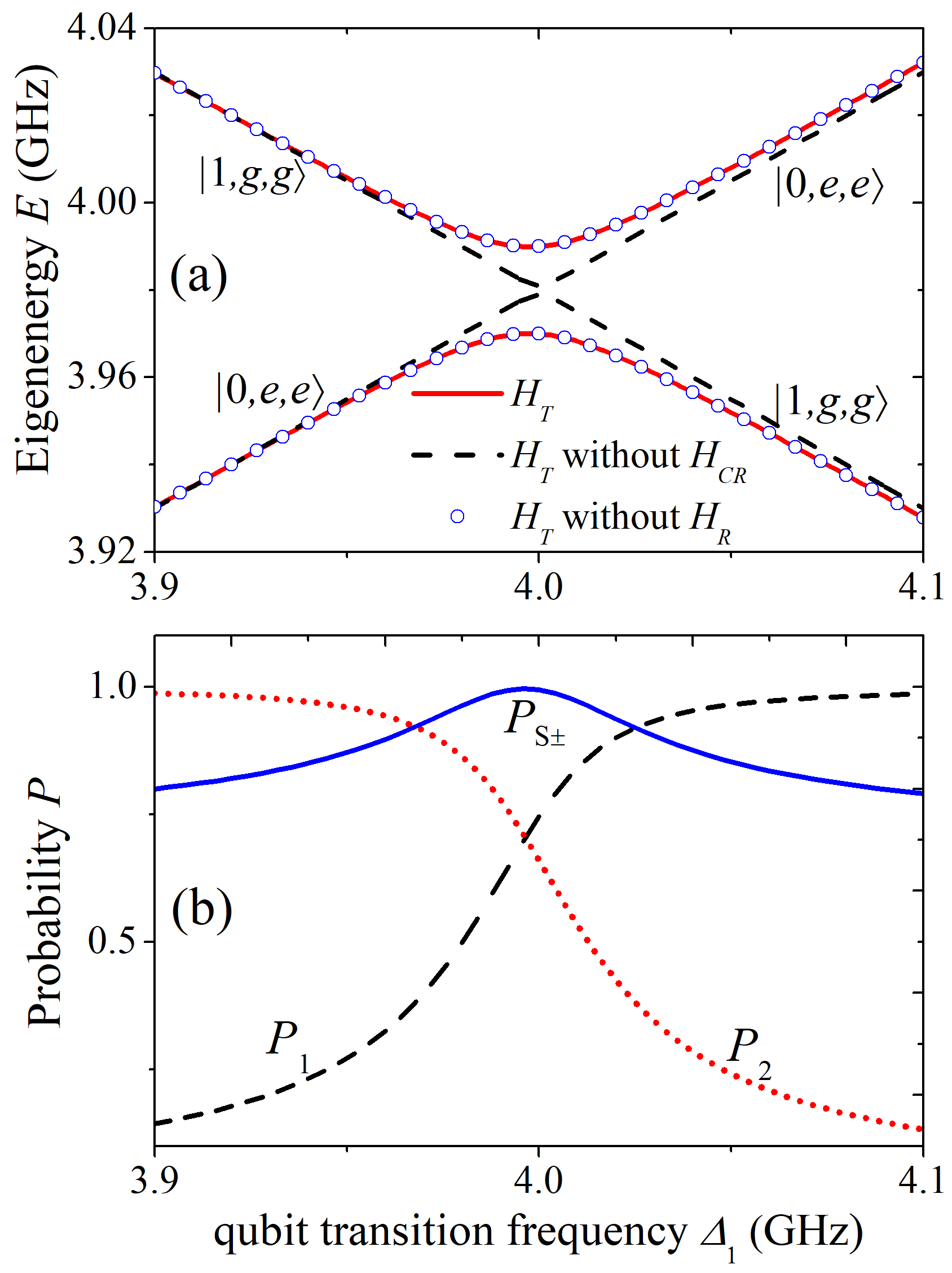
Figure 2: (Color online) (a) Eigenenergies $E_{3}$ and $E_{4}$ as functions of the first qubit transition frequency $\Delta_{1}$. Numerical results are calculated with the original Hamiltonian $H_{T}$ in Eq. (6) (red solid curve), $H_{T}$ without the counter-rotating terms $H_{\text{CR}}$ (black dashed curve), and $H_{T}$ without the resonant terms $H_{\text{R}}$ (blue dots). It can be clearly seen that the energy spectrum for $E_{3}$ and $E_{4}$ exhibits an anticrossing point around $\Delta_{1}=4~{}\text{GHz}$. The results without $H_{\text{R}}$, rather than without the counter-rotating terms $H_{\text{CR}}$, match well with those of the original Hamiltonian $H_{T}$. (b) The probabilities $P_{1}$ (black dashed curve), $P_{2}$ (red dot curve) and $P_{s\pm}$ (blue solid curve) which are defined in Sec. III A, as functions of the first qubit transition frequency $\Delta_{1}$. The parameters used here are: $\omega=2\Delta_{2}=8~{}\text{GHz}$, $g_{1}=g_{2}=0.2~{}\text{GHz}$, and $J=0.1~{}\text{GHz}$.

We are interested in the regime when $\omega\approx\Delta_{1}+\Delta_{2}$, and assume that the resonator and second-qubit frequencies are $\omega=2\Delta_{2}=8~{}\text{GHz}$. Under current experimental conditions, the coupling strength between a TLR and a qubit can easily reach the strong-coupling regime (see, Ref. Gu et al. (2017) for a recent review), and we assume that $g_{1}=g_{2}=0.2~{}\text{GHz}$. According to Ref. Majer et al. (2005), a direct inductive coupling strength between the two flux qubits can be several hundred MHz. In the following discussions, we set $J=0.1~{}\text{GHz}$ .

III.1 Anticrossing point in energy spectra

In Fig. 2(a), by changing the first atomic-transition frequency $\Delta_{1}$, we plot the energy spectrum of the third and fourth eigenenergies by numerically solving the eigenproblem $H_{T}|\psi_{n}\rangle=E_{n}|\psi_{n}\rangle$, with $n=3,4$. It can be seen that the two energy levels exhibit anticrossing with a splitting around $\Delta_{1}=4~{}\text{GHz}$ (red solid curves), which indicates that there might be two states coupled resonantly. Specifically, if the counter-rotating terms $H_{\text{CR}}$ in Eq. (6) are neglected, the anticrossing point disappears (see the dashed black curves). However, without the two-qubit resonant coupling terms $H_{\text{R}}$, the energy spectrum (blue dot curves) for the third and fourth eigenstates coincides with the full Hamiltonian case, which indicates that the resonant coupling is due to the counter-rotating terms $H_{\text{CR}}$, and has no relation with $H_{\text{R}}$. We note that the predicted level anti-crossing is analogous to that observed in the experiment of Niemczyk et al. Niemczyk et al. (2010) and other experiments in the USC regime using superconducting quantum circuits (for a very recent review see Gu et al. (2017) and references therein). Analogous to our model, the emergence of this level anticrossing needs qubit-oscillator longitudinal couplings. However, as discussed in Refs. Niemczyk et al. (2010); Garziano et al. (2015); Wang et al. (2016a), the origin of this phenomenon is due to multi-excitation processes and has a close relation to both the counter-rotating terms and JC terms in the transverse coupling. In our proposal, only the counter-rotating terms contribute to the energy level anticrossing, even far below the USC regime.

In Fig. 2(b), we plot the probabilities $P_{1}=|\langle 0,e,e|\psi_{4}\rangle|^{2}$, $P_{2}=|\langle 1,g,g|\psi_{4}\rangle|^{2}$, $P_{s+}=|\langle S_{+}|\psi_{3}\rangle|^{2}$ and $P_{s-}=|\langle S_{-}|\psi_{4}\rangle|^{2}$(where $|S_{\pm}\rangle=(|0,e,e\rangle\pm|1,g,g\rangle)/\sqrt{2}$), changing with $\Delta_{1}$. It can be seen that $|\psi_{3}\rangle\simeq|1,g,g\rangle$ ($|\psi_{4}\rangle\simeq|0,e,e\rangle$) when $\Delta_{1}\sim 3.9~{}\text{GHz}$ ($\Delta_{1}\sim 4.1~{}\text{GHz}$). Around the anticrossing point, $|S_{+}\rangle\simeq|\psi_{3}\rangle$ and $|S_{-}\rangle\simeq|\psi_{4}\rangle$. One may wonder why we are not showing in Fig. 2 the corresponding plots for the probabilities $P^{\prime}_{1}=|\langle 1,g,g|\psi_{3}\rangle|^{2}$, $P^{\prime}_{2}=|\langle 0,e,e|\psi_{3}\rangle|^{2}$, $P^{\prime}_{1}\approx P_{1}$, and $P^{\prime}_{2}\approx P_{2}$, such that we would not see any differences between the corresponding curves on the scale of Fig. 2. Therefore, we can conclude that the anticrossing point is due to the resonant coupling between the states $|0,e,e\rangle$ and $|1,g,g\rangle$. The coherent transfer between these two states corresponds to the same interesting process discussed in Ref. Garziano et al. (2016): that a single photon in a cavity can excite two atoms simultaneously. One may wonder how this process can happen in our system with only longitudinal coupling. To show this, hereafter, we analytically derive its effective Hamiltonian.

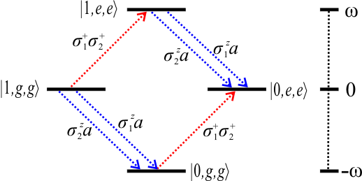
Figure 3: (Color online) Sketch of the high-order transitions between the states $|1,g,g\rangle$ and $|0,e,e\rangle$. The four transition paths, allowed by the longitudinal couplings (blue arrows) $\sigma_{j}^{z}a$ and the counter-rotating terms $\sigma_{1}^{+}\sigma_{2}^{+}$ (red arrows), are mediated by the two states $|0,g,g\rangle$ and $|1,e,e\rangle$. It is seen that the only difference between the two paths (with the same intermediate state) corresponds to different longitudinal couplings, which results in annihilating a virtual photon via the first (at the rate $\beta_{1}J$) or second (at the rate $\beta_{2}J$) qubits.

III.2 Effective Hamiltonian for the tripartite interaction

We first perform the polariton transformation of the Hamiltonian $H_{\text{tot}}$ in Eq. (6) given by

$$H_{s1}=e^{S}H_{T}e^{-S},$$ (9)

with $S=\sum_{j=1}^{2}\beta_{j}\sigma_{j}^{z}(a^{{\dagger}}-a)$, where $\beta_{j}=g_{j}/\omega$ is the Lamb-Dicke parameter for the $j$th qubit-resonator longitudinal coupling. Thus, we obtain

$$H_{s1} = \omega a^{{\dagger}}a+\frac{1}{2}\sum_{j=1}^{2}\Delta_{j}\sigma_{j}^{z}-\chi\sigma_{1}^{z}\sigma_{2}^{z}$$ (10)

$$+J\prod_{j=1}^{2}[\sigma_{j}^{+}e^{2\beta_{j}(a^{{\dagger}}-a)}+\text{H.c.}],$$

where $\chi=4g_{1}g_{2}/\omega$ is the $\sigma_{1}^{z}\sigma_{2}^{z}$ coupling strength between two qubits. Given that $\beta_{j}\ll 1$ ($\beta_{1}=\beta_{2}=0.025$), the last term in Eq. (10) can be expanded to first order in $\beta_{j}$. Therefore, $H_{s1}$ can be approximately written as

$$H_{s2} \simeq \omega a^{{\dagger}}a+\frac{1}{2}\sum_{j=1}^{2}\Delta_{j}\sigma_{j}^{z}-\chi\sigma_{1}^{z}\sigma_{2}^{z}$$ (11)

$$+ J\big{[}(\sigma_{1}^{+}+\sigma_{1}^{-})+2\beta_{1}(\sigma_{1}^{+}-\sigma_{1}^{-})(a^{{\dagger}}-a)\big{]}$$

$$\times \big{[}(\sigma_{2}^{+}+\sigma_{2}^{-})+2\beta_{2}(\sigma_{2}^{+}-\sigma_{2}^{-})(a^{{\dagger}}-a)\big{]}.$$

The last term describes various types of multi-excitation interactions among the qubits and the field, such as $\sigma_{1}^{+}\sigma_{2}^{+}a$ and $\sigma_{1}^{+}\sigma_{2}^{+}a^{2}$. To observe the effects of the counter-rotating terms in the dipole-dipole coupling, here we assume that the dipole-dipole coupling $J\ll\rm{min}\{{\Delta_{j},\Delta_{j}\pm\omega}\}$ ($j=1,2$) and $\omega=\Delta_{1}+\Delta_{2}$. Employing the commutation relations $[\sigma_{1}^{z}\sigma_{2}^{z},\sigma_{1}^{\pm}\sigma_{2}^{\pm}]=0$, and applying the unitary transformation

$$U=\exp\Big{[}-i\Big{(}\omega a^{{\dagger}}a+\frac{1}{2}\sum_{j=1}^{2}\Delta_{j}\sigma_{j}^{z}-\chi\sigma_{1}^{z}\sigma_{2}^{z}\Big{)}t\Big{]}$$ (12)

to the Hamiltonian in Eq. (11) for the time $t$, we obtain the resonant Hamiltonian by neglecting the rapidly oscillating terms

$$H_{\rm{eff}}=G_{s}(a\sigma_{1}^{+}\sigma_{2}^{+}+a^{{\dagger}}\sigma_{1}^{-}\sigma_{2}^{-}),$$ (13)

with the effective coupling strength

$$G_{s}=2J(\beta_{1}+\beta_{2})=\frac{2J(g_{1}+g_{2})}{\omega}.$$ (14)

We can clearly find that Eq. (13) describes the energy of a photon in a resonator splitting into two parts and simultaneously exciting two qubits. In the original Hamiltonian in Eq. (6), the longitudinal coupling between the $j$th qubit and the resonator, i.e., $\sigma_{j}^{z}a^{{\dagger}}$ ($\sigma_{j}^{z}a$) corresponds to the creation (annihilation) of a virtual photon in the resonator at a rapid rate $\omega$. The counter-rotating term in the qubit coupling, i.e., $\sigma_{1}^{+}\sigma_{2}^{+}$ ($\sigma_{1}^{-}\sigma_{2}^{-}$), describes the process of simultaneously exciting (de-exciting) two qubits. This term does not conserve the excitation number, and is also a virtual process oscillating at a high frequency $(\Delta_{1}+\Delta_{2})$. However, as shown in Fig. 3, these excitation-number-nonconserving processes can be combined together to form four resonant transition processes. The coherent-transfer rate between the states $|n+1,g,g\rangle$ and $|n,e,e\rangle$ is $\sqrt{n+1}G_{s}$, with $|n,g,g\rangle$ and $|n+1,e,e\rangle$ being two intermediate states, respectively. In contrast to conventional QED problems, where we neglect the counter-rotating terms, here $H_{\text{CR}}$ plays a key role in exciting the two qubits simultaneously, while the resonant terms $H_{\text{R}}$ have no effect. Therefore, the RWA is not valid here, even if the couplings are not in the ultrastrong-coupling regime.

By assuming the same parameters as in Fig. 2 and $\Delta=4~{}\rm{GHz}$, the effective coupling strength can be as strong as $G_{s}=10~{}\text{MHz}$. Compared with the results in Refs. Garziano et al. (2016); Zhao et al. (2017), there is only a single (rather than two) intermediate virtual state $|0,g,g\rangle$ during the process where a single photon excites two atoms. Consequently, the corresponding coupling rates are faster by about one order of magnitude.

III.3 Adiabatic Landau-Zener transition

In the vicinity of the anticrossing point, we first examine the adiabatic Landau-Zener transition effect Zener (1932); Rubbmark et al. (1981); Shevchenko et al. (2010) without considering the dissipative channels. Assuming that the atomic transition frequency $\Delta_{1}$ is linearly dependent in time, i.e.,

$$\Delta_{1}(t)=\Delta_{1}(0)+vt,$$ (15)

where $\Delta_{1}(t)$ sweeps through the anticrossing point at a velocity $v$. In an experiment, it is convenient to tune $\Delta_{1}(t)$ linearly by changing the flux $\Phi_{x,1}$ through the SQUID loop. We assume that the system is initially in its fourth eigenstate $|\psi_{4}\rangle\simeq|1,g,g\rangle$. When changing $\Delta_{1}(t)$ linearly, the system might jump to the lower eigenstate $|\psi_{3}\rangle$ due to the diabatic transition. In other words, this means that the system evolves far away from a quasi-steady state and transitions between different eigenstates can occur. Thus, the final transition probability to the state $|\psi_{3}\rangle\simeq|1,g,g\rangle$ ($\Delta>4~{}\rm{GHz}$) can be approximately expressed by the Landau-Zener formula Zener (1932); Rubbmark et al. (1981); Ma and Law (2015), i.e.,

$$P_{\psi_{3}}=\exp\left[{-2\pi\frac{G_{s}^{2}}{dE_{\Delta}/dt}}\right],$$ (16)

where $E_{\Delta}=E_{4}(t)-E_{3}(t)$ is the eigenenergy difference between the fourth and third eigenstates, and $dE_{\Delta}/dt$ is the sweeping rate. Here we simply have $dE_{\Delta}/dt\simeq v$. If the energy-sweeping speed $v$ is extremely slow and satisfies the relation $2\pi G_{s}^{2}\gg v$, the anticrossing point traverses adiabatically Rubbmark et al. (1981); Ma and Law (2015). In this case, the system approximately evolves along the fourth-energy curve, and the system rarely jumps to the third eigenstate after the sweeping, i.e., $P_{\psi_{3}}\ll 1$.

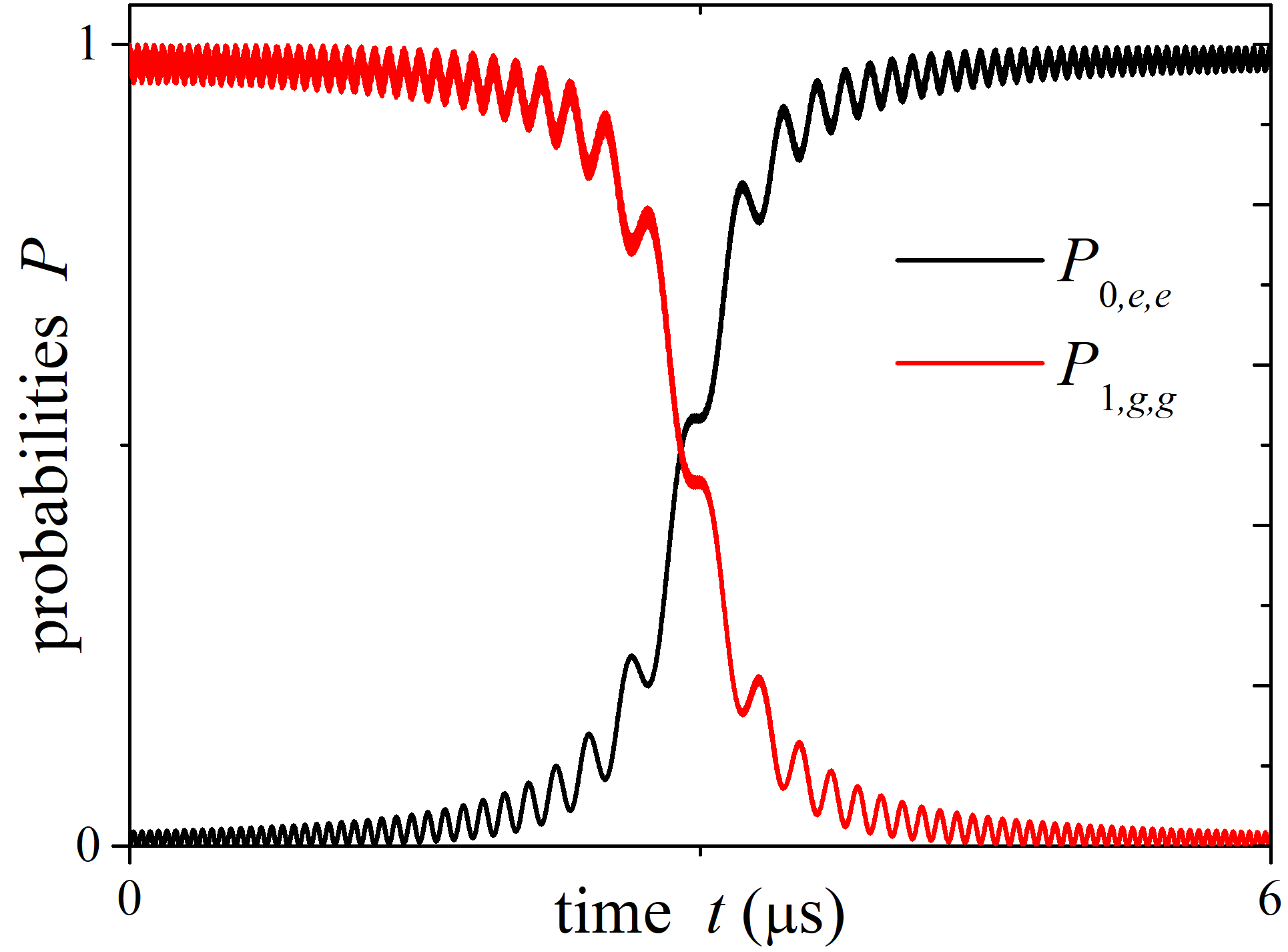
Figure 4: (Color online) The time-dependent Landau-Zener transition process is achieved by slowly changing the first-qubit frequency $\Delta_{1}$ with a sweeping rate $v=6\times 10^{-5}~{}(\text{GHz})^{2}$. The initial state is $|1,g,g\rangle$ (red curve). Due to the resonant coupling effects, the probability of the initial state is gradually decreased, and the system is adiabatically transferred into the state $|0,e,e\rangle$ (black curve) with the final probability $P_{1,e,e}\simeq 0.99$. The other parameters used here are the same as those in Fig. 2(a).

In Fig. 4, by setting $\Delta_{0}(t)=3.84~{}\text{GHz}$ and $v=6\times 10^{-5}~{}(\text{GHz})^{2}$, we numerically simulate the evolution dominated by the Schrödinger equation, and plot the probabilities of the states $|1,g,g\rangle$ and $|0,e,e\rangle$ changing with time, respectively. It can be clearly seen that the probability $P_{0,e,e}$ gradually increases from 0 to $\sim 0.99$. The transition time is of the order of several microseconds. For the final states, there is still a low probability $P_{1,g,g}$ because of the extremely-weak diabatic-transition effect Rubbmark et al. (1981). During this process, the excitation energy of a single photon is split into two parts, to effectively excite the two flux qubits. The dynamics of this Landau-Zener transition provides a strong evidence of the resonant coupling between the states $|1,g,g\rangle$ and $|0,e,e\rangle$.

IV Quantum Rabi oscillations and interference effects between four transition paths

To examine the deterministic transition between the states $|1,g,g\rangle$ and $|0,e,e\rangle$, the rate of the adiabatic Landau-Zener transition process is extremely slow. Therefore, we can simply observe the Rabi oscillation between these two states.

We assume that the resonator and two qubits are coupled to the vacuum environment and the initial states of the system are their ground states $|0,g,g\rangle$. The coherent electromagnetic field is applied via a 1D transmission line, which couples to one side of the resonator via a capacitance Underwood et al. (2012).

We can inject a single photon into the resonator by applying a Gaussian pulse, i.e., to prepare the initial state as $|1,g,g\rangle$, and the corresponding drive has the form

$$H_{\rm drv}(t)=A\frac{\exp{\left[-(t-t_{0})^{2}/(2\tau^{2})\right]}}{\sqrt{2\pi}\tau}\left(ae^{i\omega t}+a^{{\dagger}}e^{-i\omega t}\right).$$ (17)

where $A$, $t_{0}$, and $\tau$ are the amplitude, central-peak position, and width of a Gaussian pulse. However, for a resonator without nonlinearity, the higher-energy states (for example, $|2,g,g\rangle$) can also be effectively populated. We can employ an ancillary superconducting qubit to induce some nonlinearities of the resonator with a Kerr-type Hamiltonian $H_{\text{Kerr}}=\chi_{3}a^{{\dagger}2}a^{2}$ Hoffman et al. (2011); Garziano et al. (2016). Here, $\chi_{3}$ is the effective Kerr-interaction strength proportional to third-order susceptibility. As a result, the Hamiltonian for the whole system can be written as

$$H_{t}=H_{T}+H_{\text{Kerr}}+H_{\rm drv}(t).$$ (18)

IV.1 Modified input-output relation

In standard QED systems, the output and correlation signal are obtained via photodetection methods. As discussed in Refs. Ridolfo et al. (2012); Garziano et al. (2013); Ridolfo et al. (2013); Garziano et al. (2015), when the coupling is in the strong or ultrastrong coupling regimes, the eigenstates of the system are the highly-dressed states which are different from the bare eigenstates of the resonator and qubits, and the standard input-output relation fails to describe the output field. For example, the output field photon flux is not proportional to the conventional first-order correlation functions of the cavity operators any more Ridolfo et al. (2012). By contrast to this, the output field from the cavity is linked to the electric-field operator $X=a+a^{{\dagger}}$ (rather than the annihilation operator $a$) Ridolfo et al. (2012); Collett and Gardiner (1984); Gardiner and Collett (1985).

To discuss problems more explicitly and consider more general cases, we employ the modified formula of the input-output relation and correlation functions in the following discussions. Defining the positive and negative frequency Garziano et al. (2013) components of the operator $X$ as

$$X^{+}=\sum_{j,k>j}X_{jk}|\psi_{j}\rangle\langle\psi_{k}|,\quad X^{-}=(X^{+})^{{\dagger}},$$ (19)

where $X_{jk}=\langle\psi_{j}|(a+a^{{\dagger}})|\psi_{k}\rangle$, the modified input-output relation under the Markov approximation can be reexpressed as

$$A_{\text{out}}=A_{\text{in}}-\sqrt{\kappa}X^{+},$$ (20)

where $A_{\text{in}}$ is the input vacuum noise Ridolfo et al. (2012); Collett and Gardiner (1984); Gardiner and Collett (1985), $\kappa$ is the photon escape rate from the resonator Underwood et al. (2012), and $A_{\text{out}}$ is the output field operator of the form Garziano et al. (2013):

$$A_{\text{out}}(t)=\frac{1}{2\sqrt{\pi\omega\upsilon}}\int_{0}^{\infty}d\omega^{\prime}a^{\prime}(\omega^{\prime},t_{1})e^{-i\omega^{\prime}(t-t_{1})}+\rm{H.c.},$$ (21)

where $\upsilon$ is the phase velocity of the mode $\omega$, $a^{\prime}$ is the annihilation operator of the continuous mode with frequency $\omega^{\prime}$ outside the resonator. The output photon flux can be expressed as $\Theta=\kappa\langle X^{-}X^{+}\rangle$.

IV.2 Rabi oscillations based on numerically simulating the master equation

Under the Born-Markov approximation and assuming that the resonator and the qubits are coupled to the zero-temperature vacuum reservoir, the evolution for the system can be described by the master equation of the Lindblad form Ridolfo et al. (2013); Ma and Law (2015)

$$\frac{d\rho(t)}{dt}=-i[H_{t},\rho(t)]+\kappa D[X^{+}]\rho(t)+\sum_{j=1,2}\Gamma_{j}D[C_{j}^{+}]\rho(t),$$ (22)

where $D[O]\rho(t)=[2O\rho(t)O^{{\dagger}}-O^{{\dagger}}O\rho(t)-\rho(t)O^{{\dagger}}O]/2$ is the Lindblad superoperator, and $\Gamma_{j}$ is the decay rate of the $j$th qubit. Our proposal requires only longitudinal couplings between the qubits and resonator, rather than both longitudinal and transverse couplings used in Ref. Garziano et al. (2016). Thus, the flux qubits could now work at their optimal points, and the pure-dephasing rates induced by flux noise, can be minimized, as discussed in Refs. Paauw et al. (2009); Fedorov et al. (2010); Stern et al. (2014). The coherence time of a flux qubit can be of several $\mu\rm{s}$. Here we assume that $\Gamma_{1}=\Gamma_{2}=0.2~{}\text{MHz}$. In an experiment, a superconducting resonator with quality factor over $10^{4}$ can be easily fabricated Megrant et al. (2012). We consider the decay rate of the resonator to be $\kappa=0.4~{}\text{MHz}$ ($Q=2\times 10^{4}$). Therefore, under current experimental approaches, the coherent-transition rate $G_{s}$ can easily overwhelm all the decoherence channels in our proposal.

The emission field for the $j$th qubit is proportional to the zero-time delay correlation function $\langle C^{-}C^{+}\rangle$ Garziano et al. (2015), where

$$C_{j}^{+}=\sum_{i,k>i}C_{j,ik}|\psi_{i}\rangle\langle\psi_{k}|,\quad C_{j}^{-}=(C_{j}^{+})^{{\dagger}},$$ (23)

with the coefficients $C_{j,ik}=\langle\psi_{i}|(\sigma_{+}^{j}+\sigma_{-}^{j})|\psi_{k}\rangle$. It can be clearly found that the emission operator is also divided into positive and negative frequency parts. The zero-delay two-qubit correlation function

$$G_{q}^{(2)}(0)=\langle C_{1}^{-}C_{2}^{-}C_{2}^{+}C_{1}^{+}\rangle$$

is proportional to the probability that two qubits are both in their exited states Garziano et al. (2016).

In Fig. 5, we numerically calculate the photon number $\langle X^{-}X^{+}\rangle$ inside the resonator and the two-qubit correlation function $G_{q}^{(2)}(0)$ changing with time. It can be seen that, due to the Kerr-type nonlinearity, a Gaussian pulse can create a single photon in the resonator, and the photon flux can increase rapidly. When $t\gg\tau$, the pump effect of the Gaussian pulse almost vanishes, and excitation energies can be coherently transferred between the resonator and two qubits via the Rabi-oscillation process. Around $t\simeq 0.18~{}\mu\text{s}$, the two-qubit correlation function $G_{q}^{(2)}(0)$ reaches its highest value $\sim 0.96$, indicating that the two qubits are strongly correlated and both approximately in their exited states. Meanwhile the photon number $\langle X^{-}X^{+}\rangle$ reaches it lowest value, and the injected single photon is effectively converted into the excitations of two qubits. The reversible evolution between $G_{q}^{(2)}(0)$ and $\langle X^{-}X^{+}\rangle$ is due to the vacuum Rabi oscillations between the states $|1,g,g\rangle$ and $|0,e,e\rangle$. Of course, the amplitude of the oscillations gradually decreases due to the energy-decay channels.

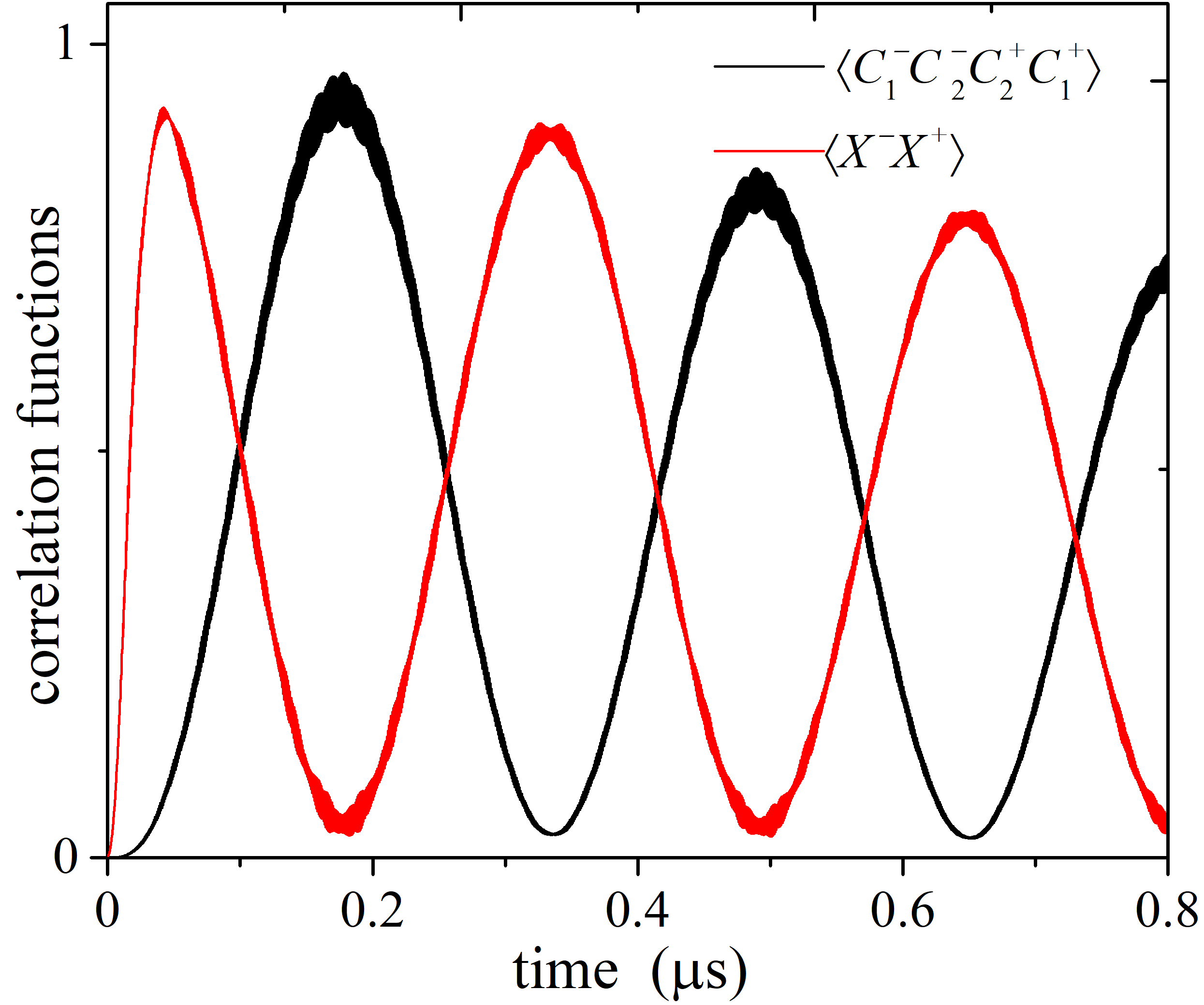
Figure 5: (Color online) The intra-resonator photon number $\langle X^{-}X^{+}\rangle$ (red curve) and zero-delay two-qubit correlation function $G_{q}^{(2)}(0)$ (black curve) versus time based on numerically solving the master equation (22) with the decay rates $\Gamma_{1}=\Gamma_{2}=0.2~{}\rm{MHz}$ and $\kappa=0.4~{}\rm{MHz}$. The Kerr nonlinearity is assumed to be $\chi_{3}=120~{}\rm{MHz}$. The initial state is $|0,g,g\rangle$. The Gaussian pulse parameters are: $t_{0}=0$, $\tau=0.02~{}\mu\rm{s}$, and $A/(\sqrt{2\pi}\tau)=50~{}\rm{MHz}$. Other parameters are the same as those in Fig. 2(a) with $\Delta_{1}=4~{}\rm{GHz}$.

IV.3 Quantum interference between four transition paths

Finally, we discuss another interesting phenomenon. As shown in Fig. 3, we can find that, for the two paths with the same intermediate state, the only difference between these paths corresponds to different longitudinal couplings, which lead to creating a virtual photon either via the first qubit ($\sigma_{1}^{z}a^{{\dagger}}$) or the second qubit ($\sigma_{2}^{z}a^{{\dagger}}$). The rates of the two paths are $G_{1}=J\beta_{1}$ and $G_{2}=J\beta_{2}$, respectively. The coherent transitions between the initial and final states can be viewed as the interference effect between these paths, i.e., $G_{s}=2(G_{1}+G_{2})$. As discussed in Sec. II, the sign and amplitude of $g_{j}$ can be easily tuned by changing the flux bias direction and the working position of the energy gap. If $g_{2}$ has opposite sign (i,e., with a $\pi$-phase difference) but the same amplitude with $g_{1}$, the paths become destructive, and the coherent transition between the states $|1,g,g\rangle$ and $|0,e,e\rangle$ vanishes. In Fig. 6(a), we plot the anticrossing gap $E_{\Delta}=E_{4}-E_{3}$ between the third and fourth eigenenergies changing with the relative strength $g_{2}/g_{1}$. It can be clearly seen that $E_{\Delta}$ has a dip (almost zero) at $g_{2}/g_{1}=-1$, indicating that the anticrossing point almost disappears. Note that $E_{\Delta}$ cannot be exactly equal to zero due to higher-order processes. At this point, the states $|1,g,g\rangle$ and $|0,e,e\rangle$ decouple from each other. When $g_{2}/g_{1}>0$, the anticrossing gap $E_{\Delta}$ increases with $g_{2}$ and the transition paths become constructive.

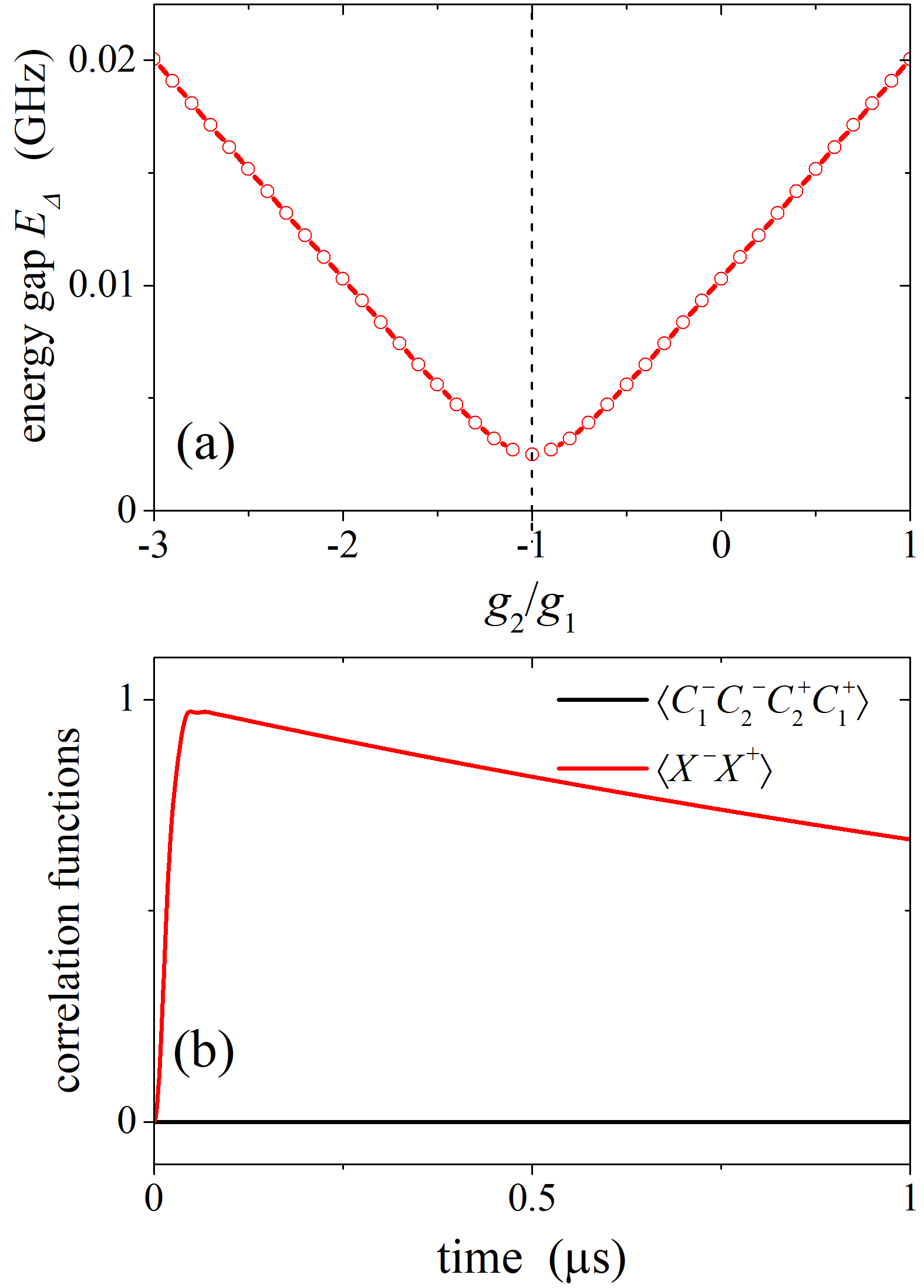
Figure 6: (Color online) (a) The energy gap (difference) between the third and fourth eigenenergies, $E_{\Delta}=E_{4}-E_{3}$, versus the relative coupling strength $g_{2}/g_{1}$ ($g_{1}=0.20~{}\text{GHz}$). At $g_{2}/g_{1}=-1$ (vertical dashed line), the gap almost vanishes. (b) Time evolutions of the photon number $\langle X^{-}X^{+}\rangle$ (red curve) and two-qubit correlation function $G_{q}^{(2)}(0)$ (black curve), which always vanishes. Here we set $g_{1}=-g_{2}=0.20~{}\text{GHz}.$ The Rabi oscillation disappears here due the destructive interference effect between the transition paths. Other parameters are the same as those in Fig. 5.

To observe more clearly the quantum destructive effects between these paths, we plot the time-dependent evolution of the photon number $\langle X^{-}X^{+}\rangle$ and the two-qubit correlation function $G_{q}^{(2)}(0)$. Here we employ the parameters at the dip in Fig. 6(a), i.e., $g_{1}=-g_{2}=0.20~{}\rm{GHz}$. As shown in Fig. 6(b), the energy cannot be transferred between the resonator and two qubits any more, which is different from the Rabi oscillation in Fig. 5. Consequently, a single photon, which is excited by a Gaussian pulse, decays to the vacuum environment (red curve), and the two-qubit correlation function $G_{q}^{(2)}(0)$ is always zero (black curves). In such conditions, the coherent transfer between the states $|1,g,g\rangle$ and $|0,e,e\rangle$ vanishes due to the destructive effect, and the counter-rotating-term effect (that a single photon excites two qubits simultaneously) cannot be observed. Therefore, in an experiment, we can simply change the relative sign and amplitude of the flux sensitivity $R_{j}$ to observe either destructive or constructive interference effects caused by the counter-rotating terms.

V Discussion and conclusions

In this paper, we have investigated pure effects of the counter-rotating terms in the dipole-dipole coupling between two superconducting qubits. The theoretical analysis shows that when these two qubits are longitudinally coupled with the same resonator, the energy of a single photon can effectively excite two qubits simultaneously. By discussing the anticrossing points around the resonant regime, we find that this coherent transition process results from the counter-rotating terms, and has no relation to the resonant coupling terms between two qubits. In fact, our results throughout this paper show that when dealing with a QED system containing longitudinal couplings, we should examine the energy spectrum of the system carefully before adopting the standard RWA. The counter-rotating terms might play an important role in the physical dynamics of the whole system.

Moreover, we have demonstrated the Landau-Zener transition effects and Rabi oscillations between the states $|1,g,g\rangle$ and $|0,e,e\rangle$, which are clear signatures of the resonant coupling between these two states. The energy of a single photon can be divided to simultaneously excite two qubits via the longitudinal couplings and the counter-rotating terms. Moreover, this process is combined with four transition paths, and there can be quantum interference between these paths. We discussed how to control the system to achieve either destructive or constructive interference effects. By discussing the experimentally feasible parameters, we find it is possible to implement our proposal and observe these quantum effects based on current state-of-the-art circuit-QED systems.

In fact, if we consider a more general case with $n\omega=\Delta_{1}+\Delta_{2}$ when deriving the resonant terms in Eq. (11), we can expand this formula to its $n$th order. In such conditions, a more general resonant Hamiltonian

$$H^{(n)}_{\rm{eff}}=G_{s}^{(n)}[a^{n}\sigma_{1}^{+}\sigma_{2}^{+}+(a^{{\dagger}})^{n}\sigma_{1}^{-}\sigma_{2}^{-}],$$ (24)

which describes higher-order effects when $n$ photons excite two qubits simultaneously, might produce observable quantum effects. However, we should note that the effective rate $G_{s}^{(n)}$ decreases quickly with increasing $n$, which might be overwhelmed by the nonresonant-oscillating terms and decoherence processes.

We should emphasize that our proposal here can be a convenient platform to observe pure quantum effects of the counter-rotating terms. As we discussed above, these high-order transitions only contain a single intermediate state, and the rate is much faster compared with the proposals in Refs. Garziano et al. (2016); Zhao et al. (2017). Therefore, the tripartite interaction in Eq. (13) provides a novel way to prepare a type of Greenberger-Horne-Zeilinger (GHZ) state Greenberger et al. (1990), $(|1,g,g\rangle+|0,e,e\rangle)/\sqrt{2}$ (see Fig. 5). Moreover, if we can prepare two qubits in their excited states, a single photon output jointly emitted by two qubits can also be obtained via this method. Therefore, this proposal might also be exploited for quantum information processing (including error correction codes Stassi et al. (2017)) and quantum optics in the microwave regime.

References

- Bloch and Siegert (1940) F. Bloch and A. Siegert, “Magnetic resonance for nonrotating fields,” Phys. Rev. 57, 522 (1940).
- Jaynes and Cummings (1963) E. T. Jaynes and F. W. Cummings, “Comparison of quantum and semiclassical radiation theories with application to the beam maser,” Proc. IEEE 51, 89 (1963).
- Shore and Knight (1993) B. W. Shore and P. L. Knight, “The Jaynes-Cummings model,” J. Mod. Opt. 40, 1195–1238 (1993).
- Irish (2007) E. K. Irish, “Generalized rotating-wave approximation for arbitrarily large coupling,” Phys. Rev. Lett. 99, 173601 (2007).
- Scully and Zubairy (1997) M. O. Scully and M. S. Zubairy, Quantum Optics (Cambridge University Press, Cambridge, 1997).
- Anappara et al. (2009) A. A. Anappara, S. De Liberato, A. Tredicucci, C. Ciuti, G. Biasiol, L. Sorba, and F. Beltram, “Signatures of the ultrastrong light-matter coupling regime,” Phys. Rev. B 79, 201303 (2009).
- Forn-Díaz et al. (2010) P. Forn-Díaz, J. Lisenfeld, D. Marcos, J. J. García-Ripoll, E. Solano, C. J. P. M. Harmans, and J. E. Mooij, “Observation of the Bloch-Siegert shift in a qubit-oscillator system in the ultrastrong coupling regime,” Phys. Rev. Lett. 105, 237001 (2010).
- Niemczyk et al. (2010) T. Niemczyk et al., “Circuit quantum electrodynamics in the ultrastrong-coupling regime,” Nat. Phys. 6, 772 (2010).
- Geiser et al. (2012) M. Geiser, F. Castellano, G. Scalari, M. Beck, L. Nevou, and J. Faist, “Ultrastrong coupling regime and plasmon polaritons in parabolic semiconductor quantum wells,” Phys. Rev. Lett. 108, 106402 (2012).
- Scalari et al. (2012) G. Scalari et al., “Ultrastrong coupling of the cyclotron transition of a 2D electron gas to a THz metamaterial,” Science 335, 1323 (2012).
- Baust et al. (2016) A. Baust et al., “Ultrastrong coupling in two-resonator circuit QED,” Phys. Rev. B 93, 214501 (2016).
- Forn-Díaz et al. (2017) P. Forn-Díaz, J. J. García-Ripoll, B. Peropadre, J.-L. Orgiazzi, M A Yurtalan, R Belyansky, C M Wilson, and A Lupaşcu, “Ultrastrong coupling of a single artificial atom to an electromagnetic continuum in the nonperturbative regime,” Nat. Phys. 13, 39 (2017).
- Yoshihara et al. (2017) F. Yoshihara, T. Fuse, S. Ashhab, K. Kakuyanagi, S. Saito, and K. Semba, “Superconducting qubit-oscillator circuit beyond the ultrastrong-coupling regime,” Nat. Phys. 13, 44 (2017).
- Chen et al. (2017) Z. Chen et al., “Single-photon-driven high-order sideband transitions in an ultrastrongly coupled circuit-quantum-electrodynamics system,” Phys. Rev. A 96, 012325 (2017).
- Braak (2011) D. Braak, “Integrability of the Rabi model,” Phys. Rev. Lett. 107, 100401 (2011).
- Gu et al. (2017) X. Gu, A. F. Kockum, A. Miranowicz, Y.-X. Liu, and F. Nori, “Microwave photonics with superconducting quantum circuits,” Phys. Rep. 718-719, 1 (2017).
- Ashhab and Nori (2010) S. Ashhab and F. Nori, “Qubit-oscillator systems in the ultrastrong-coupling regime and their potential for preparing nonclassical states,” Phys. Rev. A 81, 042311 (2010).
- Cao et al. (2010) X. Cao, J. Q. You, H. Zheng, A. G. Kofman, and F. Nori, “Dynamics and quantum Zeno effect for a qubit in either a low- or high-frequency bath beyond the rotating-wave approximation,” Phys. Rev. A 82, 022119 (2010).
- Cao et al. (2011) X. Cao, J. Q. You, H. Zheng, and F. Nori, “A qubit strongly coupled to a resonant cavity: asymmetry of the spontaneous emission spectrum beyond the rotating wave approximation,” New J. Phys. 13, 073002 (2011).
- Cao et al. (2012) X. Cao, Q. Ai, C.-P. Sun, and F. Nori, “The transition from quantum Zeno to anti-Zeno effects for a qubit in a cavity by varying the cavity frequency,” Phys. Lett. A 376, 349 (2012).
- Casanova et al. (2010) J. Casanova, G. Romero, I. Lizuain, J. J. García-Ripoll, and E. Solano, “Deep strong coupling regime of the Jaynes-Cummings model,” Phys. Rev. Lett. 105, 263603 (2010).
- Garziano et al. (2015) L. Garziano, R. Stassi, V. Macrì, A. F. Kockum, S. Savasta, and F. Nori, “Multiphoton quantum Rabi oscillations in ultrastrong cavity QED,” Phys. Rev. A 92, 063830 (2015).
- Wang et al. (2016a) X. Wang, A. Miranowicz, H.-R. Li, and F. Nori, “Multiple-output microwave single-photon source using superconducting circuits with longitudinal and transverse couplings,” Phys. Rev. A 94, 053858 (2016a).
- Ma and Law (2015) K. K. W. Ma and C. K. Law, “Three-photon resonance and adiabatic passage in the large-detuning Rabi model,” Phys. Rev. A 92, 023842 (2015).
- Ridolfo et al. (2012) A. Ridolfo, M. Leib, S. Savasta, and M. J. Hartmann, “Photon blockade in the ultrastrong coupling regime,” Phys. Rev. Lett. 109, 193602 (2012).
- Ridolfo et al. (2013) A. Ridolfo, S. Savasta, and M. J. Hartmann, “Nonclassical radiation from thermal cavities in the ultrastrong coupling regime,” Phys. Rev. Lett. 110, 163601 (2013).
- Hwang et al. (2015) M.-J. Hwang, R. Puebla, and M. B. Plenio, “Quantum phase transition and universal dynamics in the Rabi model,” Phys. Rev. Lett. 115, 180404 (2015).
- Kockum et al. (2017a) A. F. Kockum, V. Macrì, L. Garziano, S. Savasta, and F. Nori, “Frequency conversion in ultrastrong cavity QED,” Sci. Rep. 7 (2017a).
- Hwang et al. (2016) M.-J. Hwang, M.-S. Kim, and M.-S. Choi, “Recurrent delocalization and quasiequilibration of photons in coupled systems in circuit quantum electrodynamics,” Phys. Rev. Lett. 116, 153601 (2016).
- Le Boité et al. (2016) A. Le Boité, M.-J. Hwang, H. Nha, and M. B. Plenio, “Fate of photon blockade in the deep strong-coupling regime,” Phys. Rev. A 94, 033827 (2016).
- Denk et al. (1990) W. Denk, J. H. Strickler, and W. W. Webb, “Two-photon laser scanning fluorescence microscopy,” Science 248, 73 (1990).
- So et al. (2000) P. T. C. So, C. Y. Dong, B. R. Masters, and K. M. Berland, “Two-photon excitation fluorescence microscopy,” Annu. Rev. Biomed. Eng. 2, 399 (2000).
- Garziano et al. (2016) L. Garziano, V. Macrì, R. Stassi, O. Di Stefano, F. Nori, and S. Savasta, “One photon can simultaneously excite two or more atoms,” Phys. Rev. Lett. 117, 043601 (2016).
- Kockum et al. (2017b) A. F. Kockum, A. Miranowicz, V. Macrì, S. Savasta, and F. Nori, “Deterministic quantum nonlinear optics with single atoms and virtual photons,” Phys. Rev. A 95, 063849 (2017b).
- Stassi et al. (2017) R. Stassi, V. Macrì, A. F. Kockum, O. Di Stefano, A. Miranowicz, S. Savasta, and F. Nori, “Quantum nonlinear optics without photons,” Phys. Rev. A 96, 023818 (2017).
- Zhao et al. (2017) P. Zhao, X.-S. Tan, H.-F. Yu, S.-L. Zhu, and Y. Yu, “Simultaneously exciting two atoms with photon-mediated Raman interactions,” Phys. Rev. A 95, 063848 (2017).
- Fedorov et al. (2010) A. Fedorov, A. K. Feofanov, P. Macha, P. Forn-Díaz, C. J. P. M. Harmans, and J. E. Mooij, “Strong coupling of a quantum oscillator to a flux qubit at its symmetry point,” Phys. Rev. Lett. 105, 060503 (2010).
- Stern et al. (2014) M. Stern, G. Catelani, Y. Kubo, C. Grezes, A. Bienfait, D. Vion, D. Esteve, and P. Bertet, “Flux qubits with long coherence times for hybrid quantum circuits,” Phys. Rev. Lett. 113, 123601 (2014).
- Makhlin et al. (2001) Y. Makhlin, G. Schön, and A. Shnirman, “Quantum-state engineering with Josephson-junction devices,” Rev. Mod. Phys. 73, 357 (2001).
- You and Nori (2005) J. Q. You and F. Nori, “Superconducting circuits and quantum information,” Phys. Today 58, 42 (2005).
- Liu et al. (2005a) Y.-X. Liu, J. Q. You, L. F. Wei, C. P. Sun, and F. Nori, “Optical selection rules and phase-dependent adiabatic state control in a superconducting quantum circuit,” Phys. Rev. Lett. 95, 087001 (2005a).
- Clarke and Wilhelm (2008) J. Clarke and F. K. Wilhelm, “Superconducting quantum bits,” Nature (London) 453, 1031 (2008).
- DiCarlo et al. (2010) L. DiCarlo et al., “Preparation and measurement of three-qubit entanglement in a superconducting circuit,” Nature (London) 467, 574 (2010).
- You and Nori (2011) J. Q. You and F. Nori, “Atomic physics and quantum optics using superconducting circuits,” Nature (London) 474, 589 (2011).
- Buluta et al. (2011) I. Buluta, S. Ashhab, and F. Nori, “Natural and artificial atoms for quantum computation,” Rep. Prog. Phys. 74, 104401 (2011).
- Xiang et al. (2013) Z. L. Xiang, S. Ashhab, J. Q. You, and F. Nori, “Hybrid quantum circuits: Superconducting circuits interacting with other quantum systems,” Rev. Mod. Phys. 85, 623 (2013).
- Georgescu et al. (2014) I. M. Georgescu, S. Ashhab, and F. Nori, “Quantum simulation,” Rev. Mod. Phys. 86, 153 (2014).
- van der Wal et al. (2000) C. H. van der Wal et al., “Quantum superposition of macroscopic persistent-current states,” Science 290, 773 (2000).
- Liu et al. (2005b) Y.-X. Liu, L. F. Wei, and F. Nori, “Tomographic measurements on superconducting qubit states,” Phys. Rev. B 72, 014547 (2005b).
- Neeley et al. (2008) M. Neeley et al., “Process tomography of quantum memory in a Josephson-phase qubit coupled to a two-level state,” Nat. Phys. 4, 523 (2008).
- Chen et al. (2011) Y. F. Chen, D. Hover, S. Sendelbach, L. Maurer, S. T. Merkel, E. J. Pritchett, F. K. Wilhelm, and R. McDermott, “Microwave photon counter based on Josephson junctions,” Phys. Rev. Lett. 107, 217401 (2011).
- Inomata et al. (2016) K. Inomata, Z. R. Lin, K. Koshino, W. D. Oliver, J. S. Tsai, T. Yamamoto, and Y. Nakamura, “Single microwave-photon detector using an artificial -type three-level system,” Nat. Commun. 7, 12303 (2016).
- Sillanpää et al. (2009) M. A. Sillanpää, J. Li, K. Cicak, F. Altomare, J. I. Park, R. W. Simmonds, G. S. Paraoanu, and P. J. Hakonen, “Autler-Townes effect in a superconducting three-level system,” Phys. Rev. Lett. 103, 193601 (2009).
- Wang et al. (2016b) X. Wang, H.-R. Li, D.-X. Chen, W.-X. Liu, and F.-L. Li, “Tunable electromagnetically induced transparency in a composite superconducting system,” Opt. Commun. 366, 321 (2016b).
- Gu et al. (2016) X. Gu, S.-N. Huai, F. Nori, and Y.-X. Liu, “Polariton states in circuit QED for electromagnetically induced transparency,” Phys. Rev. A 93, 063827 (2016).
- Hofheinz et al. (2008) M. Hofheinz et al., “Generation of Fock states in a superconducting quantum circuit,” Nature (London) 454, 310 (2008).
- Hofheinz et al. (2009) M. Hofheinz et al., “Synthesizing arbitrary quantum states in a superconducting resonator,” Nature 459, 546 (2009).
- Premaratne et al. (2017) S. P. Premaratne, F. C. Wellstood, and B. S. Palmer, “Microwave photon Fock state generation by stimulated Raman adiabatic passage,” Nat. Commun. 8, 14148 (2017).
- Blais et al. (2004) A. Blais, R.-S. Huang, A. Wallraff, S. M. Girvin, and R. J. Schoelkopf, “Cavity quantum electrodynamics for superconducting electrical circuits: An architecture for quantum computation,” Phys. Rev. A 69, 062320 (2004).
- Mooij et al. (1999) J. E. Mooij, T. P. Orlando, L. Levitov, L. Tian, C. H. Van der Wal, and S. Lloyd, “Josephson persistent-current qubit,” Science 285, 1036 (1999).
- Orlando et al. (1999) T. P. Orlando, J. E. Mooij, L. Tian, C. H. van der Wal, L. S. Levitov, S. Lloyd, and J. J. Mazo, “Superconducting persistent-current qubit,” Phys. Rev. B 60, 15398 (1999).
- You et al. (2007) J. Q. You, Y. X. Liu, C. P. Sun, and F. Nori, “Persistent single-photon production by tunable on-chip micromaser with a superconducting quantum circuit,” Phys. Rev. B 75, 104516 (2007).
- Paauw et al. (2009) F. G. Paauw, A. Fedorov, C. J. P. M Harmans, and J. E. Mooij, “Tuning the gap of a superconducting flux qubit,” Phys. Rev. Lett. 102, 090501 (2009).
- Niskanen et al. (2006) A. O. Niskanen, K. Harrabi, F. Yoshihara, Y. Nakamura, and J. S. Tsai, “Spectroscopy of three strongly coupled flux qubits,” Phys. Rev. B 74, 220503 (2006).
- et al. (2006) M. Grajcar et al., “Four-qubit device with mixed couplings,” Phys. Rev. Lett. 96, 047006 (2006).
- Harris et al. (2009) R. Harris et al., “Compound Josephson-junction coupler for flux qubits with minimal crosstalk,” Phys. Rev. B 80, 052506 (2009).
- Averin and Bruder (2003) D. V. Averin and C. Bruder, “Variable electrostatic transformer: Controllable coupling of two charge qubits,” Phys. Rev. Lett. 91, 057003 (2003).
- Wallquist et al. (2005) M. Wallquist, J. Lantz, V. S. Shumeiko, and G. Wendin, “Superconducting qubit network with controllable nearest-neighbour coupling,” New J. Phys. 7, 178 (2005).
- Harris et al. (2007) R. Harris et al., “Sign- and magnitude-tunable coupler for superconducting flux qubits,” Phys. Rev. Lett. 98, 177001 (2007).
- Tsomokos et al. (2010) D. I. Tsomokos, S. Ashhab, and F. Nori, “Using superconducting qubit circuits to engineer exotic lattice systems,” Phys. Rev. A 82, 052311 (2010).
- Yurke and Denker (1984) B. Yurke and J. S. Denker, “Quantum network theory,” Phys. Rev. A 29, 1419 (1984).
- Clerk et al. (2010) A. A. Clerk, M. H. Devoret, S. M. Girvin, F. Marquardt, and R. J. Schoelkopf, “Introduction to quantum noise, measurement, and amplification,” Rev. Mod. Phys. 82, 1155 (2010).
- Majer et al. (2005) J. B. Majer, F. G. Paauw, A. C. J. ter Haar, C. J. P. M. Harmans, and J. E. Mooij, “Spectroscopy on two coupled superconducting flux qubits,” Phys. Rev. Lett. 94, 090501 (2005).
- Zener (1932) C. Zener, “Non-adiabatic crossing of energy levels,” Proc. R. Soc. London 137, 696 (1932).
- Rubbmark et al. (1981) J. R. Rubbmark, M. M. Kash, M. G. Littman, and D. Kleppner, “Dynamical effects at avoided level crossings: A study of the Landau-Zener effect using Rydberg atoms,” Phys. Rev. A 23, 3107 (1981).
- Shevchenko et al. (2010) S. N. Shevchenko, S Ashhab, and F. Nori, “Landau-Zener-Stückelberg interferometry,” Phys. Rep. 492, 1 (2010).
- Underwood et al. (2012) D. L. Underwood, W. E. Shanks, Jens Koch, and A. A. Houck, “Low-disorder microwave cavity lattices for quantum simulation with photons,” Phys. Rev. A 86, 023837 (2012).
- Hoffman et al. (2011) A. J. Hoffman, S. J. Srinivasan, S. Schmidt, L. Spietz, J. Aumentado, H. E. Türeci, and A. A. Houck, “Dispersive photon blockade in a superconducting circuit,” Phys. Rev. Lett. 107, 053602 (2011).
- Garziano et al. (2013) L. Garziano, A. Ridolfo, R. Stassi, O. Di Stefano, and S. Savasta, “Switching on and off of ultrastrong light-matter interaction: Photon statistics of quantum vacuum radiation,” Phys. Rev. A 88, 063829 (2013).
- Collett and Gardiner (1984) M. J. Collett and C. W. Gardiner, “Squeezing of intracavity and traveling-wave light fields produced in parametric amplification,” Phys. Rev. A 30, 1386 (1984).
- Gardiner and Collett (1985) C. W. Gardiner and M. J. Collett, “Input and output in damped quantum systems: Quantum stochastic differential equations and the master equation,” Phys. Rev. A 31, 3761 (1985).
- Megrant et al. (2012) A. Megrant et al., “Planar superconducting resonators with internal quality factors above one million,” Appl. Phys. Lett. 100, 113510 (2012).
- Greenberger et al. (1990) D. M. Greenberger, M. A. Horne, A. Shimony, and A. Zeilinger, “Bell’s theorem without inequalities,” Am. J. Phys. 58, 1131 (1990).