On the support of the Kloosterman paths

Abstract.

We obtain statistical results on the possible distribution of all partial sums of a Kloosterman sum modulo a prime, by computing explicitly the support of the limiting random Fourier series of our earlier functional limit theorem for Kloosterman paths.

1. Introduction

Let $p$ be a prime number. For $(a,b)\in{\mathbf{F}^{\times}_{p}}\times{\mathbf{F}^{\times}_{p}}$, we denote

$$\operatorname{Kl}_{2}(a,b;p)=\frac{1}{\sqrt{p}}\sum_{x\in{\mathbf{F}^{\times}_{p}}}e\Bigl{(}\frac{ax+b\bar{x}}{p}\Bigr{)}$$

(where $e(z)=e^{2i\pi z}$ for $z\in\mathbf{C}$) the normalized Kloosterman sums modulo $p$. As in our previous paper [15], we consider the Kloosterman paths $t\mapsto K_{p}(a,b)(t)$ for $0\leqslant t\leqslant 1$, namely the random variables on the finite set ${\mathbf{F}^{\times}_{p}}\times{\mathbf{F}^{\times}_{p}}$ obtained by linearly interpolating the partial sums

$$(a,b)\mapsto\frac{1}{\sqrt{p}}\sum_{1\leqslant x\leqslant j}e\Bigl{(}\frac{ax+b\bar{x}}{p}\Bigr{)},\quad\quad 0\leqslant j\leqslant p-1$$

that correspond to $t=j/(p-1)$ (see [15, §1]). The set ${\mathbf{F}^{\times}_{p}}\times{\mathbf{F}^{\times}_{p}}$ is viewed as a probability space with the uniform probability measure, denoted $\mathbf{P}_{p}$.

We proved [15, Th. 1.1, Th. 1.5] that as $p\to+\infty$, the $C([0,1])$-valued random variables $K_{p}$ converge in law to the random Fourier series

$$\mathrm{K}(t)=t\mathrm{ST}_{0}+\sum_{h\not=0}\frac{e(ht)-1}{2\pi ih}\mathrm{ST}_{h}$$

where $(\mathrm{ST}_{h})_{h\in\mathbf{Z}}$ is a family of independent Sato-Tate random variables (i.e., with law given by $\displaystyle{\frac{1}{\pi}}\sqrt{1-\displaystyle{\frac{x^{2}}{4}}}\,dx$ on $[-2,2$]) and the convergence holds almost surely in the sense of uniform convergence of symmetric partial sums.

We discuss in this paper the support of this random Fourier series $\mathrm{K}(t)$, and the arithmetic consequences of its structure. We will denote the support by $\mathcal{S}$.

Theorem 1.1.

The support $\mathcal{S}$ of the law of $\mathrm{K}$ in $C([0,1])$ is the set of all $f\in C([0,1])$ such that $f(0)=0$, $f(1)\in[-2,2]$ and such that the function $g(t)=f(t)-tf(1)$ satisfies $\widehat{g}(h)\in i\mathbf{R}$ and

$$|\widehat{g}(h)|\leqslant\frac{1}{\pi|h|}$$

for all non-zero $h\in\mathbf{Z}$, where

$$\widehat{g}(h)=\int_{0}^{1}g(t)e(-ht)dt$$

are the Fourier coefficients of $g$.

See Section 2 for the proof. From the arithmetic point of view, what matters is the combination of this result of the next proposition.

Proposition 1.2.

Let $f\in C([0,1])$ be a function in the support $\mathcal{S}$ of $\mathrm{K}$. For any $\varepsilon>0$, we have

$$\liminf_{p\to+\infty}\frac{1}{(p-1)^{2}}\Bigl{|}\Bigl{\{}(a,b)\in{\mathbf{F}^{\times}_{p}}\times{\mathbf{F}^{\times}_{p}}\,\mid\,\\ \max_{0\leqslant j\leqslant p-1}\Bigl{|}\frac{1}{\sqrt{p}}\sum_{1\leqslant x\leqslant j}e\Bigl{(}\frac{ax+b\bar{x}}{p}\Bigr{)}-f\Bigl{(}\frac{j}{p-1}\Bigr{)}\Bigr{|}<\varepsilon\Bigr{\}}\Bigr{|}>0.$$

Conversely, if $\in C([0,1])$ does not belong to $\mathcal{S}$, then there exists $\delta>0$ such that

$$\lim_{p\to+\infty}\frac{1}{(p-1)^{2}}\Bigl{|}\Bigl{\{}(a,b)\in{\mathbf{F}^{\times}_{p}}\times{\mathbf{F}^{\times}_{p}}\,\mid\,\\ \max_{0\leqslant j\leqslant p-1}\Bigl{|}\frac{1}{\sqrt{p}}\sum_{1\leqslant x\leqslant j}e\Bigl{(}\frac{ax+b\bar{x}}{p}\Bigr{)}-f\Bigl{(}\frac{j}{p-1}\Bigr{)}\Bigr{|}<\delta\Bigr{\}}\Bigr{|}=0.$$

As an example, we obtain:

Corollary 1.3.

For any $\varepsilon>0$, we have

$$\liminf_{p\to+\infty}\frac{1}{(p-1)^{2}}\Bigl{|}\Bigl{\{}(a,b)\in{\mathbf{F}^{\times}_{p}}\times{\mathbf{F}^{\times}_{p}}\,\mid\,\max_{0\leqslant j\leqslant p-1}\Bigl{|}\frac{1}{\sqrt{p}}\sum_{1\leqslant x\leqslant j}e\Bigl{(}\frac{ax+b\bar{x}}{p}\Bigr{)}\Bigr{|}<\varepsilon\Bigr{\}}\Bigr{|}>0.$$

Our goal, after proving these results, will be to illustrate them. We begin in Section 3 by spelling out some properties of the support of $\mathrm{K}$, some of which can be interpreted as “hidden symmetries” of the Kloosterman paths. Then we discuss some concrete examples that we find interesting, especially various polygonal paths in Section 5. In Section 6, we consider functions not in $\mathcal{S}$ which can be brought to $\mathcal{S}$ by change of variable. We can show:

Proposition 1.4.

Let $f\in C([0,1])$ be a real-valued function such that $f(t)+f(1-t)=f(1)$ for all $t\in[0,1]$ and $|f(1)|\leqslant 2$. Then there exists an increasing homeomorphism $\varphi\colon[0,1]\to[0,1]$ such that $\varphi(1-t)=1-\varphi(t)$ for all $t$ and $f\circ\varphi\in\mathcal{S}$.

We will see that this is related to some classical problems of Fourier analysis around the Bohr-Pál Theorem.

We also highlight two questions for which we do not know the answer at this time, and one interesting analogue problem:

1. Is there a space-filling curve in the support $\mathcal{S}$ of $\mathrm{K}$?

2. Does Proposition 1.4 hold for complex-valued functions $f$ with $f(t)+\overline{f(1-t)}=f(1)$? (A positive answer would also give a positive answer to (1)).

3. What can be said about the support of the paths of partial character sums (as in, e.g., the paper [5] of Bober, Goldmakher, Granville and Koukoulopoulos)?

Acknowledgments. The computations were performed using Pari/GP [20] and Julia [10]; the plots were produced using the Gadfly.jl package.

Notation.

We denote by $|X|$ the cardinality of a set. If $X$ is any set and $f\colon X\to\mathbf{C}$ any function, we write (synonymously) $f\ll g$ for $x\in X$, or $f=O(g)$ for $x\in X$, if there exists a constant $C\geqslant 0$ such that $|f(x)|\leqslant Cg(x)$ for all $x\in X$. The “implied constant” is any admissible value of $C$. It may depend on the set $X$ which is always specified or clear in context.

We denote by $C([0,1])$ the space of all continuous complex-valued functions on $[0,1]$.

For any probability space $(\Omega,\Sigma,\mathbf{P})$, we denote by $\mathbf{P}(A)$ the probability of some event $A$, and for a $\mathbf{C}$-valued random variable $X$ defined on $\Omega$, we denote by $\mathbf{E}(X)$ the expectation when it exists. We sometimes use different probability spaces, but often keep the same notation for all expectations and probabilities.

2. Computation of the support

We begin with the proof of Theorem 1.1. This uses a standard probabilistic lemma, for which we include a proof for completeness.

Lemma 2.1.

Let $B$ be a separable real or complex Banach space. Let $(X_{n})_{n\geqslant 1}$ be a sequence of independent $B$-valued random variables such that the series $X=\sum X_{n}$ converges almost surely. The support of the law of $X$ is the closure of the set of all convergent series of the form $\sum x_{n}$, where $x_{n}$ belongs to the support of the law of $X_{n}$ for all $n\geqslant 1$.

Proof.

For $N\geqslant 1$, we write

$$S_{N}=\sum_{n=1}^{N}X_{n},\quad\quad R_{N}=X-S_{N}.$$

The variables $S_{N}$ and $R_{N}$ are independent. It is elementary (by composition of the random vector $(X_{1},\ldots,X_{N})$ with the continuous addition map) that the support of $S_{N}$ is the closure of the set of elements $x_{1}+\cdots+x_{N}$ with $x_{n}\in\operatorname{supp}(X_{n})$ for $1\leqslant n\leqslant N$.

We will prove that all convergent series $\sum x_{n}$ with $x_{n}\in\operatorname{supp}(X_{n})$ belong to the support of $X$, hence the closure of this set is contained in the support of $X$. Thus let $x=\sum x_{n}$ be of this type. Let $\varepsilon>0$ be fixed.

For all $N$ large enough, we have

$$\Bigl{\|}\sum_{n>N}x_{n}\Bigr{\|}<\varepsilon,$$

and it follows that $x_{1}+\cdots+x_{N}$ belongs to the intersection of the support of $S_{N}$ (by the previous remark) and of the open ball $U_{\varepsilon}$ of radius $\varepsilon$ around $x$. Hence

$$\mathbf{P}(S_{N}\in U_{\varepsilon})>0$$

for all $N$ large enough.

Now the almost sure convergence implies (by the dominated convergence theorem, for instance) that $\mathbf{P}(\|R_{N}\|>\varepsilon)\rightarrow 0$ as $N\rightarrow+\infty$. Therefore, taking $N$ suitably large, we get

$$\mathbf{P}(\|X-x\|<2\varepsilon) \geqslant\mathbf{P}(\|S_{N}-x\|<\varepsilon\text{ and }\|R_{N}\|<\varepsilon)$$

$$=\mathbf{P}(\|S_{N}-x\|<\varepsilon)\mathbf{P}(\|R_{N}\|<\varepsilon)>0$$

(by independence). Since $\varepsilon$ is arbitrary, this shows that $x\in\operatorname{supp}(X)$, as was to be proved.

The converse inclusion (which we do not need anyway) is elementary since for any $n$, we have $\mathbf{P}(X_{n}\notin\operatorname{supp}(X_{n}))=0$. ∎

This almost immediately proves Theorem 1.1, but some care is needed since not all continuous periodic functions are the sum of their Fourier series in $C([0,1]$).

Proof of Theorem 1.1.

Denote by $\widetilde{\mathcal{S}}$ the set described in the statement. Then $\widetilde{\mathcal{S}}$ is closed in $C([0,1])$, since it is the intersection of closed sets. Almost surely, a sample function $f\in C([0,1])$ of the random process $\mathrm{K}$ is given by a uniformly convergent series

$$f(t)=\alpha_{0}t+\sum_{h\not=0}\frac{e(ht)-1}{2\pi ih}\alpha_{h}$$

(in the sense of symmetric partial sums) for some real numbers $\alpha_{h}$ such that $|\alpha_{h}|\leqslant 2$ ([15, Th. 1.1 (1)]). The uniform convergence implies

$$\widehat{g}(h)=\frac{\alpha_{h}}{2i\pi h},\quad\text{ where }\quad g(t)=f(t)-tf(1),$$

for $h\not=0$. Hence the function $f$ belongs to $\widetilde{\mathcal{S}}$. Consequently, the support of $\mathrm{K}$ is contained in $\widetilde{\mathcal{S}}$.

We now prove the converse inclusion. By Lemma 2.1, the support $\mathcal{S}$ contains the set of continuous functions with uniformly convergent (symmetric) expansions

$$t\alpha_{0}+\sum_{h\not=0}\frac{e(ht)-1}{2\pi ih}\alpha_{h}$$

where $\alpha_{h}\in[-2,2]$ for all $h\in\mathbf{Z}$. In particular, since $0$ belongs to the support of the Sato-Tate measure, $\mathcal{S}$ contains all finite sums of this type.

Let $f\in\widetilde{\mathcal{S}}$. We have

$$g(t)=f(t)-tf(1)=\lim_{N\to+\infty}\sum_{|h|\leqslant N}\widehat{g}(h)e(ht)\Bigl{(}1-\frac{|h|}{N}\Bigr{)},$$

in $C([0,1])$, by the uniform convergence of Cesàro means of the Fourier series of a continuous periodic function. Evaluating at $0$, where $g(0)=0$, and subtracting yields

$$f(t) =tf(1)+\lim_{N\to+\infty}\sum_{|h|\leqslant N}\widehat{g}(h)(e(ht)-1)\Bigl{(}1-\frac{|h|}{N}\Bigr{)}$$

$$=tf(1)+\lim_{N\to+\infty}\sum_{|h|\leqslant N}\frac{\alpha_{h}}{2i\pi h}(e(ht)-1)\Bigl{(}1-\frac{|h|}{N}\Bigr{)}$$

in $C([0,1])$, where $\alpha_{h}=2i\pi h\widehat{g}(h)$ for $h\not=0$. Then $\alpha_{h}\in\mathbf{R}$ and $|\alpha_{h}|\leqslant 2$ by the assumption that $f\in\widetilde{\mathcal{S}}$, so each function

$$tf(1)+\sum_{1\leqslant|h|\leqslant N}\frac{e(ht)-1}{2\pi ih}\alpha_{h}\Bigl{(}1-\frac{|h|}{N}\Bigr{)},$$

belongs to $\mathcal{S}$, by the result we recalled. Since $\mathcal{S}$ is closed, we conclude that $f$ also belongs to $\mathcal{S}$. ∎

We now prove the arithmetic statement of Proposition 1.2.

Proof of Proposition 1.2.

Assume $f\in\mathcal{S}$. Since the $C([0,1])$-valued random variables $K_{p}$ converge in law to $\mathrm{K}$ as $p\to+\infty$ ([15, Th. 1.5]), a standard equivalent form of convergence in law implies that for any open set $U\subset C([0,1])$, we have

$$\liminf_{p\to+\infty}\mathbf{P}_{p}(K_{p}\in U)\geqslant\mathbf{P}(\mathrm{K}\in U)$$

(see [3, Th. 2.1, (i) and (iv)]). If $f\in\mathcal{S}$ and $U$ is an open neighborhood of $f$ in $C([0,1])$, then by definition we have $\mathbf{P}(\mathrm{K}\in U)>0$, and therefore

$$\liminf_{p\to+\infty}\mathbf{P}_{p}(K_{p}\in U)\geqslant\mathbf{P}(\mathrm{K}\in U)>0.$$

Take for $U$ the open ball of radius $\varepsilon>0$ around $f$ so that $K_{p}\in U$ if and only if

$$\sup_{t\in[0,1]}|K_{p}(t)-f(t)|<\varepsilon.$$

Sampling the supremum at the points $t_{j}=j/(p-1)$ for $0\leqslant j\leqslant p-1$, we deduce

$$\liminf_{p\to+\infty}\mathbf{P}_{p}\Bigl{(}\Bigl{|}K_{p}\Bigl{(}\frac{j}{p-1}\Bigr{)}-f\Bigl{(}\frac{j}{p-1}\Bigr{)}\Bigr{|}<\varepsilon\Bigr{)}>0,$$

which translates exactly to the first statement.

Conversely, if $f\notin\mathcal{S}$, there exists a neighborhood $U$ of $f$ such that $\mathbf{P}(\mathrm{K}\in U)=0$. For some $\delta>0$, this neighborhood contains the closed ball $C$ of radius $\delta$ around $f$, and by [3, Th. 2.1., (i) and (iii)], we have

$$0\leqslant\limsup_{p\to+\infty}\mathbf{P}_{p}(K_{p}\in C)\leqslant\mathbf{P}(\mathrm{K}\in C)=0,$$

hence the second assertion. ∎

3. Structure and symmetries of the support

We denote by $u$ the continuous linear map $C([0,1])\to C([0,1])$ such that

$$u(f)(t)=f(t)-f(1)t$$

for all $t\in[0,1]$.

Let $\mathcal{{F}}_{0}\subset C([0,1])$ denote the real Banach space of all complex-valued continuous functions on $[0,1]$ such that

(3.1) $$f(t)+\overline{f(1-t)}=f(1)$$

for all $t\in[0,1]$. This condition implies (taking $t=1/2$) that $2\operatorname{Re}(f(1/2))=f(1)$, hence in particular that $f(1)\in\mathbf{R}$. Taking $t=0$, it follows also that $f(0)=0$. Writing the symmetry relation (3.1) as

(3.2) $$f(t)-\operatorname{Re}(f({\textstyle{\frac{1}{2}}}))=-\overline{f(1-t)}+\operatorname{Re}(f({\textstyle{\frac{1}{2}}})),$$

we see also that $\mathcal{{F}}_{0}$ is the subspace of functions satisfying $f(0)=0$ among the space $\mathcal{{F}}$ of all complex-valued continuous functions $f$ on $[0,1]$ that satisfy (3.2). This means, in particular, that the image $f([0,1])\subset\mathbf{C}$ is symmetric with respect to the line $\operatorname{Re}(z)={\textstyle{\frac{1}{2}}}\operatorname{Re}(f(1))$ in $\mathbf{C}$.

The linear map $u$ induces by restriction an $\mathbf{R}$-linear map $u\colon\mathcal{{F}}_{0}\to\mathcal{{F}}_{0}$. This is a continuous projection on $\mathcal{{F}}_{0}$ with $1$-dimensional kernel spanned by the identity $t\mapsto t$, and with image the subspace $\mathcal{{F}}_{1}\subset\mathcal{{F}}_{0}$ of functions such that $f(1)=0$.

Theorem 1.1 implies that $\mathcal{S}\subset\mathcal{{F}}_{0}$, where the symmetry condition (3.1) follows from the fact that the Fourier coefficients of the function $g=u(f)$ are purely imaginary. More precisely, we have the following criterion that we will use to check that concretely given functions in $\mathcal{{F}}_{0}$ are in $\mathcal{S}$:

Lemma 3.1.

Let $f\in C([0,1])$. Then $f\in\mathcal{{F}}_{0}$ if and only if there exist real numbers $\alpha_{h}$ for $h\in\mathbf{Z}$ such that

$$f(t)=\alpha_{0}t+\lim_{N\to+\infty}\sum_{1\leqslant|h|\leqslant N}\alpha_{h}\frac{e(ht)-1}{2i\pi h}\Bigl{(}1-\frac{|h|}{N}\Bigr{)}.$$

uniformly for $t\in[0,1]$.

For $f$ in $\mathcal{{F}}_{0}$, the expansion above holds if and only if

$$\alpha_{0}=f(1),\quad\quad\alpha_{h}=f(1)+2i\pi h\widehat{f}(h)\quad\text{ for }h\not=0.$$

We have then $f\in\mathcal{S}$ if and only if $|\alpha_{h}|\leqslant 2$ for all $h\in\mathbf{Z}$.

Proof.

This is a variant of part of the proof of Theorem 1.1. The “if” statement follows from the uniform convergence by computation of the Fourier coefficients. For the “only if” statement, consider any $f\in\mathcal{{F}}_{0}$, and write $u(f)$ as the uniform limit of its Cesàro means; evaluating at $t=0$ and using $u(f)(0)=0$, we obtain

$$f(t)=\alpha_{0}t+\lim_{N\to+\infty}\sum_{1\leqslant|h|\leqslant N}\alpha_{h}\frac{e(ht)-1}{2i\pi h}\Bigl{(}1-\frac{|h|}{N}\Bigr{)}.$$

with $\alpha_{0}=f(1)$ and $\alpha_{h}=f(1)+2i\pi h\widehat{f}(h)$ for $h\not=0$. The symmetry $f(t)+\overline{f(1-t)}=f(1)$ then shows that $\alpha_{h}\in\mathbf{R}$.

The remaining statements are then elementary. ∎

The support $\mathcal{S}$ has some symmetry properties that we now describe:

1. The support $\mathcal{S}$ of $\mathrm{K}$ is a subset of $\mathcal{{F}}_{0}$. It is closed, convex and balanced (i.e., if $f\in\mathcal{S}$ and $\alpha\in[-1,1]$, then we have $\alpha f\in\mathcal{S}$, see [6, EVT, I, p. 6, déf. 3]). In particular, if $f$ is in $\mathcal{S}$, then $-f$ is also in $\mathcal{S}$.

2. We have $\bar{f}\in\mathcal{S}$ if $f\in\mathcal{S}$. In particular, we deduce that if $f\in\mathcal{S}$, then $\operatorname{Re}(f)={\textstyle{\frac{1}{2}}}(f+\bar{f})$ and $i\operatorname{Im}(f)={\textstyle{\frac{1}{2}}}(f-\bar{f})$ are also in $\mathcal{S}$; on the other hand, $\operatorname{Im}(f)\in\mathcal{S}$ only if $f$ is real-valued (so the imaginary is zero).

3. Denote by $\mathcal{S}_{1}$ the intersection of $\mathcal{S}$ and $\mathcal{{F}}_{1}$, i.e., those $f\in\mathcal{S}$ with $f(1)=0$. Then $f\in\mathcal{S}$ if and only if $u(f)\in\mathcal{S}_{1}$ and $f(1)\in[-2,2]$. In particular, we have a kind of “action” of $[-2,2]$ on $\mathcal{S}$: given $f\in\mathcal{S}$ and $\alpha\in\mathbf{R}$ such that $-2\leqslant\alpha+f(1)\leqslant 2$, the function given by $f_{\alpha}(t)=\alpha t+f(t)$ belongs to $\mathcal{S}$ (and $f_{\alpha+\beta}(t)=(f_{\alpha})_{\beta}$, when this makes sense).

4. The support $\mathcal{S}$ is “stable under Fourier contractions”: given any subset $S$ of $\mathbf{Z}$ and any $f\in\mathcal{S}$, if a function $g\in\mathcal{{F}}_{0}$ satisfies $|g(1)|\leqslant|f(1)|$ and $|\widehat{u(g)}(h)|\leqslant|\widehat{u(f)}(h)|$ for alll $h\not=0$ in $\mathbf{Z}$, then $g\in\mathcal{S}$.

These are all immediate consequences of the description of $\mathcal{S}$. However, from the point of view of Kloosterman paths, they are by no means obvious, and reflect hidden symmetry properties of the “shapes” of Kloosterman sums.

The next remarks describe some “obvious” elements of $\mathcal{S}$.

1. By a simple integration by parts, the support $\mathcal{S}$ contains all functions $f$ such that $f(1)\in[-2,2]$ and $u(f)$ is in $C^{1}([0,1])\cap\mathcal{{F}}_{0}$ with $\|f^{\prime}\|_{\infty}\leqslant 2$. More generally, it suffices that $u(f)$ be of total variation with the total variation of $u(f)$ at most $2$.

2. Let $g\colon[0,1]\to\mathbf{R}$ be a real-valued continuous function such that $g(0)=0$ and $g(1-t)=g(t)$ for all $t$. Then for any $\alpha$ with $|\alpha|\leqslant 2$, the function

   $$f(t)=\alpha t+ig(t)$$

   (whose image is, for $\alpha=1$, the graph of $f$) is in $\mathcal{{F}}_{0}$; it belongs to $\mathcal{S}$ if and only if the non-zero Fourier coefficients of $g=u(f)/i$ satisfy

   $$|\widehat{g}(f)|\leqslant\frac{1}{\pi|h|}.$$

3. Let $\mathcal{{G}}\subset\mathcal{{F}}_{0}$ be the real subspace of functions $f\in\mathcal{F}_{0}$ such that we have

   $$\|f\|_{\mathcal{{G}}}=\sup_{h\in\mathbf{Z}}|h\widehat{u(f)}(h)|<+\infty,$$

   given the corresponding structure of Banach space (note that the only constant function in $\mathcal{{G}}$ is the zero function to see that this is a norm). This space contains all $C^{1}$ functions that belong to $\mathcal{{F}}_{0}$ (in fact, it contains all functions $f$ of bounded variation, and $\|f\|_{\mathcal{{G}}}$ is bounded by the total variation of $f$ by [25, Th. II.4.12]). We have $\mathcal{S}\subset\mathcal{{G}}$, and $\mathcal{S}$ is the closed ball of radius $\pi^{-1}$ centered at $0$ in $\mathcal{{G}}$. In particular, for any $f\in\mathcal{{G}}$, there exists $\alpha>0$ such that $\alpha f\in\mathcal{S}$. From the arithmetic point of view, this means that any smooth enough curve satisfying the “obvious” symmetry condition can be approximated by Kloosterman paths, after re-scaling it to bring the value at $1$ and the Fourier coefficients in the right interval.

The support $\mathcal{S}$ of $\mathrm{K}$ is, in any reasonable sense, a very “small” subset of the subspace $\mathcal{{F}}_{0}$ of $C([0,1])$. For instance, the natural analogue of the Wiener measure on $\mathcal{{F}}_{0}$ is the series

$$\mathrm{N}(t)=tN_{0}+\sum_{h\not=0}\frac{e(ht)-1}{2\pi ih}N_{h}$$

where $(N_{h})$ are independent standard (real) gaussian random variables. It is elementary that the support of $\mathrm{N}$ is $\mathcal{{F}}_{0}$, whereas we have $\mathbf{P}(N\in\mathcal{S})=0$.

This sparsity property of $\mathcal{S}$ means that the Kloosterman paths (as parameterized paths) are rather special, and may explain why they seem experimentally rather distinctive (at least to certain eyes). More importantly maybe, this feature raises a number of interesting questions that are simply irrelevant for Brownian motion or Wiener measure: given some “natural” $f\in\mathcal{{F}}_{0}$, does it belong to $\mathcal{S}$ or not? This also contrasts with results like Bagchi’s Theorem for the functional distribution of (say) vertical translates of the Riemann zeta function, where the support of the limiting distribution is “as large as possible”, given obvious restrictions (see [1] and [14, §3.2, 3.3]; but see also Remark 5.2 to see that there are interesting issues there also).

Another subtlety is that the question might be phrased in different ways. A picture of a Kloosterman path, as in [15], only shows the image $f([0,1])$ of a function $f\in\mathcal{{F}}_{0}$, and therefore different functions lead to the same picture (we may replace $f$ by $f\circ\varphi$ for any homeomorphism $\varphi\colon[0,1]\to[0,1]$ such that $\varphi(0)=0$ and $\varphi(1-t)=1-\varphi(t)$, which implies that $f\circ\varphi$ is also in $\mathcal{{F}}_{0}$). So even if a function $f\in\mathcal{{F}}_{0}$ does not belong to $\mathcal{S}$, we can ask whether there exists a reparameterization $\varphi$ such that $f\circ\varphi\in\mathcal{S}$. Following this question leads to connections with some classical problems of Fourier analysis, as we discuss in Section 6.

Finally, we remark that the support of $\mathrm{K}$ only depends on the support of the Sato-Tate summand, and not on their particular distribution. This implies that $\mathcal{S}$ is also the support of similar random Fourier series where the summands are independent and have support $[-2,2]$. In particular, from the work of Ricotta and Royer [21], this applies to the support of the random Fourier series that appears as limit in law of the Kloosterman paths modulo $p^{n}$ for fixed $n\geqslant 1$ and $p\to+\infty$, where the corresponding Fourier series has summands $\mathrm{C}_{h}$ distributed like the trace of a random matrix in the normalizer of the diagonal torus in $\operatorname{SU}_{2}(\mathbf{C})$. (Note however that the values of the liminf and limsup in Proposition 1.2 do, of course, depend on the laws on the summands).

4. Elementary examples

We present here a number of examples, in the spirit of curiosity. Before we begin, we remark that since numerical inequalities are important in determining whether a function $f\in C([0,1])$ belongs to the support of $\mathrm{K}$, we have “tested” the following computations by making, in each case, sample checks with Pari/GP to detect multiplicative normalization errors.

Example 4.1.

Take $f(t)=\alpha t$ for some real number $\alpha$ with $|\alpha|\leqslant 2$. Then $f$ visibly belongs to the support of $\mathrm{K}(t)$ since $u(f)=0$.

In particular, for $\alpha=0$, we get Corollary 1.3 from Proposition 1.2: for any $\varepsilon>0$, we have

$$\liminf_{p\to+\infty}\frac{1}{(p-1)^{2}}\Bigl{|}\Bigl{\{}(a,b)\in{\mathbf{F}^{\times}_{p}}\times{\mathbf{F}^{\times}_{p}}\,\mid\,\max_{0\leqslant j\leqslant p-1}\Bigl{|}\frac{1}{\sqrt{p}}\sum_{1\leqslant x\leqslant j}e\Bigl{(}\frac{ax+b\bar{x}}{p}\Bigr{)}\Bigr{|}<\varepsilon\Bigr{\}}\Bigr{|}>0.$$

So it is possible for the partial sums of the normalized Kloosterman sum to remain at all time in an arbitrarily small neighborhood of the origin.

Example 4.2.

Take $f(t)=i\alpha t(1-t)$ for some real number $\alpha$. Then $f\in\mathcal{{F}}_{0}$. We compute (using Lemma 3.1) the coefficients $\alpha_{h}$ in the expansion

$$f(t)=\alpha_{0}t+\lim_{N\to+\infty}\sum_{1\leqslant|h|\leqslant N}\alpha_{h}\frac{e(ht)-1}{2i\pi h}\Bigl{(}1-\frac{|h|}{N}\Bigr{)},$$

and find that $\alpha_{0}=0$ and $\alpha_{h}=\alpha(\pi h)^{-1}\in\mathbf{R}$ for all $h\not=0$. In particular, we have $|\alpha_{h}|\leqslant 2$ for all $h$ if and only if $|\alpha|\leqslant 2\pi$.

The graph of $f$ in that case is the vertical segment $[0,i\alpha/4]$. So this parameterized segment $[0,iR]$ can be approximated by the graph of a Kloosterman path as long as $|R|\leqslant\pi/2$. More precisely, Proposition 1.2 gives

$$\liminf_{p\to+\infty}\frac{1}{(p-1)^{2}}\Bigl{|}\Bigl{\{}(a,b)\in{\mathbf{F}^{\times}_{p}}\times{\mathbf{F}^{\times}_{p}}\,\mid\,\\ \max_{0\leqslant j\leqslant p-1}\Bigl{|}\frac{1}{\sqrt{p}}\sum_{1\leqslant x\leqslant j}e\Bigl{(}\frac{ax+b\bar{x}}{p}\Bigr{)}-i\alpha\frac{j}{p-1}\Bigl{(}1-\frac{j}{p-1}\Bigr{)}\Bigr{|}<\varepsilon\Bigr{\}}\Bigr{|}>0,$$

if $|\alpha|\leqslant\pi/2$.

Example 4.3.

Let $\alpha\in[-1,1]$ and consider the map

$$f_{1}(t)=2\alpha t+i\sqrt{\alpha^{2}-\alpha^{2}(2t-1)^{2}},$$

which parameterizes a semicircle above the real axis with diameter $[0,2\alpha]$. The function $f_{1}$ belongs to $\mathcal{{F}}_{0}$.

Let $\varphi_{1}=u(f_{1})$. We have

$$\varphi_{1}(t)=i\sqrt{\alpha^{2}-\alpha^{2}(2t-1)^{2}},$$

and using the computation of the Fourier transform of a semicircle distribution (see, e.g., [8, 3.752 (2)]), we find

$$\widehat{\varphi}_{1}(h)=\alpha(-1)^{h}\frac{J_{1}(\pi h)}{2h},$$

for $h\not=0$, where $J_{1}$ is the Bessel function of the first kind. From Bessel’s integral representation

$$J_{1}(x)=\frac{1}{2\pi}\int_{0}^{2\pi}\cos(t-x\sin(t))dt,$$

(see, e.g., [24, p. 19]) we see immediately that $|J_{1}(x)|\leqslant 1$ for all $x$ (in fact, the maximal value of the Bessel function is about $0.58186$), hence the bound $|\widehat{\varphi}_{1}(h)|\leqslant(\pi|h|)^{-1}$ holds for all $h\not=0$, and therefore $f_{1}$ belongs to the support of $\mathrm{K}$ for $|\alpha|\leqslant 1$.

Now we consider a second parameterization of the same half circle, namely

$$f_{2}(t)=2\alpha(1-\cos(\pi t)+i\sin(\pi t)),$$

(more precisely, this is below the real axis if $\alpha<0$). Let $\varphi_{2}=u(f_{2})$. We compute

$$\widehat{\varphi}_{2}(h)=2\alpha\Bigl{(}\frac{1}{i\pi h}-\frac{1}{i\pi(h+{\textstyle{\frac{1}{2}}})}\Bigr{)},$$

from which it follows that $f_{2}$ also belongs to the support of $\mathrm{K}$.

We see in particular here that the Kloosterman sum can follow this semicircle in at least two ways…

Example 4.4.

For $t\in\mathbf{R}$, let $\langle t\rangle$ denote the distance to the nearest integer. The Takagi function $\tau$ is the real-valued function defined on $[0,1]$ by

$$\tau(t)=\sum_{j\geqslant 0}\frac{\langle 2^{j}t\rangle}{2^{j}}.$$

It is continuous and nowhere differentiable, and has many remarkable properties, including intricate self-similarity (see, e.g., the survey by Lagarias [16]). Since $\tau(1-t)=\tau(t)$ for $t\in[0,1]$ and $\tau(1)=0$, the function $f$ giving the graph of $\tau$, namely

$$f(t)=t+i\tau(t),$$

belongs to $\mathcal{{F}}_{0}$. Hata and Yamaguti computed the Fourier coefficients of $\tau$, from which it follows that

$$\widehat{u(f)}(h)=\frac{1}{2^{m}k^{2}i\pi^{2}}$$

for $h\not=0$, when one writes $|h|=2^{m}k$ with $k$ an odd integer (see, e.g., [16, Th. 6.1]). Hence

$$|\widehat{u(f)}(h)|\leqslant\frac{1}{2^{m}k\pi^{2}}\leqslant\frac{1}{\pi^{2}|h|},$$

and we can conclude that $f\in\mathcal{S}$. An approximation of the graph of $\tau$ is plotted in Figure 1.

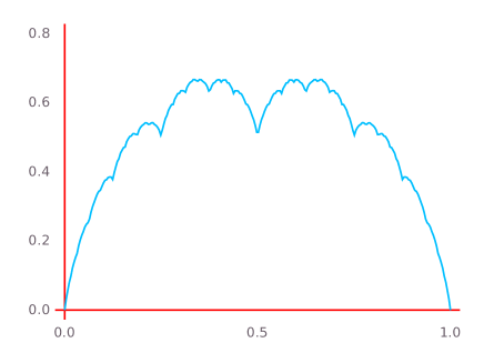
Figure 1. The Takagi function

Example 4.5.

Another famous function of real-analysis is Riemann’s Fourier series

$$\varrho(t)=\sum_{n\geqslant 1}\frac{1}{\pi n^{2}}\sin(\pi n^{2}t).$$

This is a real-valued continuous $2$-periodic function such that $\varrho(0)=0$ and $\varrho(t)+\varrho(2-t)=0$ for all $t$. It is non-differentiable except at rational points $r=a/b$ with $a$ and $b$ coprime odd integers, where $\varrho^{\prime}(r)=-1/2$ (this is due to Hardy for non-differentiability at irrational $t$, and to Gerver for rational points; see Duistermaat’s survey [7], which focuses on the links between $\varrho$ and the classical theta function). Define $f(t)=\varrho(2t)$. Then $f$ is a real-valued element of $\mathcal{{F}}_{0}$ with $u(f)=f$, and $\widehat{f}(h)=0$ if $|h|$ is not a square, while

$$\widehat{f}(\varepsilon h^{2})=\frac{\varepsilon}{2i\pi h^{2}}$$

for all $h\geqslant 1$ and $\varepsilon\in\{-1,1\}$. Therefore $f\in\mathcal{S}$. In Figure 2 is the graph of $f$ (not the path described by $f$, which is simply a segment of $\mathbf{R}$).

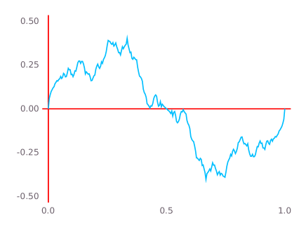
Figure 2. The Riemann function

Example 4.6.

Yet another familiar example is the Cantor staircase function $\gamma$, which can be defined as $\gamma(t)=\mathbf{P}(X\leqslant t)$, where $X$ is the random series

$$X=\sum_{k\geqslant 1}X_{k}$$

with $(X_{k})$ a sequence of independent random variables such that

$$\mathbf{P}(X_{k}=0)=\mathbf{P}\Bigl{(}X_{k}=\frac{2}{3^{k}}\Bigr{)}=\frac{1}{2}$$

for $k\geqslant 1$.

The Cantor function satisfies $\gamma(0)=0$, $\gamma(1)=1$ and $\gamma(t)+\gamma(1-t)=1$ for all $t$, hence $\gamma$ is a real-valued element of $\mathcal{{F}}_{0}$. Computing using the probabilistic definition, we obtain quickly the formula

$$\widehat{u(\gamma)}(h)=\frac{(-1)^{h}}{2i\pi h}\prod_{k\geqslant 1}\cos\Bigl{(}\frac{2\pi h}{3^{k}}\Bigr{)},$$

from which we see that $\gamma\in\mathcal{S}$.

Example 4.7.

Let

$$f(t)=\sum_{h\geqslant 1}\mu(h)\frac{e(ht)-1}{2i\pi},$$

where $\mu(h)$ denotes the Möbius function. It is known (essentially from work of Davenport, see [2] and [11, Th 13.6], and from the Prime Number Theorem that implies that $\sum\mu(h)h^{-1}=0$) that the series converges uniformly. Clearly this function, which we call the Davenport function, belongs to $\mathcal{S}$. Its path is pictured in the left-hand graph of Figure 3.

We may replace the Möbius function with the Liouville function, and we also display the resulting path on the right-hand side of Figure 3.

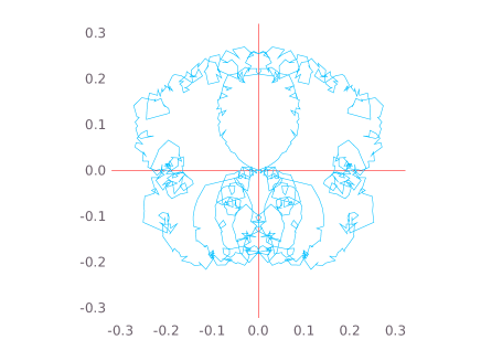
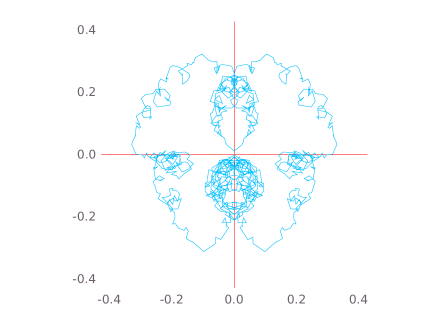
Figure 3. The Davenport function and its variant

5. Polygonal paths

Polygonal paths provide a very natural class of examples of functions, and we will consider a number of them. We begin with some elementary preparation.

Let $z_{0}$ and $z_{1}$ be complex numbers, and $t_{0}<t_{1}$ real numbers. We define $\Delta=t_{1}-t_{0}$ and $f\in C([0,1])$ by

$$f(t)=\begin{cases}\frac{1}{\Delta}(z_{1}(t-t_{0})+z_{0}(t_{1}-t))&\text{ if }t_{0}\leqslant t\leqslant t_{1},\\ 0&\text{ otherwise,}\end{cases}$$

which parameterizes the segment from $z_{0}$ to $z_{1}$ during the interval $[t_{0},t_{1}]$.

Let $h\not=0$ be an integer. By direct computation, we find

$$\widehat{f}(h) =-\frac{1}{2i\pi h}(z_{1}e(-ht_{1})-z_{0}e(-ht_{0}))+\frac{1}{2i\pi h}(z_{1}-z_{0})e(-ht_{0})\frac{1}{\Delta}\Bigl{(}\int_{0}^{\Delta}e(-hu)du\Bigr{)}$$

$$=-\frac{1}{2i\pi h}(z_{1}e(-ht_{1})-z_{0}e(-ht_{0}))+\frac{1}{2i\pi h}(z_{1}-z_{0})\frac{\sin(\pi h\Delta)}{\pi h\Delta}e\Bigl{(}-h\Bigl{(}t_{0}+\frac{\Delta}{2}\Bigr{)}\Bigr{)}.$$

Consider now an integer $n\geqslant 1$, a family $(z_{0},\ldots,z_{n})$ of complex numbers and a family $(t_{0},\ldots,t_{n})$ of real numbers with

$$0=t_{0}<t_{1}<\ldots<t_{n-1}<t_{n}=1.$$

Let $f_{j}$ be the function as above relative to the points $(z_{j},z_{j+1})$ and the interval $[t_{j},t_{j+1}]$, and let function

$$f=\sum_{j=0}^{n-1}f_{j}$$

(in other words, $f$ parameterizes the polygonal path joining $z_{0}$ to $z_{1}$ to … to $z_{n}$, over intervals $[t_{0},t_{1}]$, …, $[t_{n-1},t_{n}]$). Let $\Delta_{j}=t_{j+1}-t_{j}$.

For $h\not=0$, we obtain by summing the previous expression, and using a telescoping sum

(5.1) $$\widehat{f}(h)=-\frac{1}{2i\pi h}(z_{n}-z_{0})+\frac{1}{2i\pi h}\sum_{j=0}^{n-1}(z_{j+1}-z_{j})e\Bigl{(}-h\Bigl{(}t_{j}+\frac{\Delta_{j}}{2}\Bigr{)}\Bigr{)}\frac{\sin(\pi h\Delta_{j})}{\pi h\Delta_{j}}.$$

Now assume further that $\Delta_{j}$ is constant for $0\leqslant j\leqslant n-1$, equal to $1/n$. We then have $t_{j}=j/n$, and we obtain

(5.2) $$\widehat{f}(h)=-\frac{1}{2i\pi h}(z_{n}-z_{0})+\frac{1}{2i\pi h}\frac{\sin(\pi h/n)}{\pi h/n}\sum_{j=0}^{n-1}(z_{j+1}-z_{j})e\Bigl{(}-\frac{h(j+{\textstyle{\frac{1}{2}}})}{n}\Bigr{)}.$$

It is elementary that $f$ belongs to $\mathcal{{F}}_{0}$ if and only if $z_{0}=0$ and if the sums

(5.3) $$\widetilde{f}(h)=\sum_{j=0}^{n-1}(z_{j+1}-z_{j})e\Bigl{(}-\frac{h(j+{\textstyle{\frac{1}{2}}})}{n}\Bigr{)}$$

are real-valued. If this is the case, then the polygonal function $f$ belongs to $\mathcal{S}$ if and only if $|z_{n}|\leqslant 2$ and

(5.4) $$\Bigl{|}\frac{\sin(\pi h/n)}{\pi h/n}\widetilde{f}(h)\Bigr{|}=\Bigl{|}\frac{\sin(\pi h/n)}{\pi h/n}\sum_{j=0}^{n-1}(z_{j+1}-z_{j})e\Bigl{(}-\frac{hj}{n}\Bigr{)}\Bigr{|}\leqslant 2$$

for all $h\not=0$ (disregarding the constant phase $e(-h/(2n))$, although it is important to ensure that the exponential sums are real-valued).

Example 5.1.

The first polygonal paths that we consider are – naturally enough – the Kloosterman paths themselves.

Fix an odd prime $p$ and integers $a$ and $b$ coprime to $p$. Let $f\in C([0,1])$ be the function given by the Kloosterman path $K_{p}(a,b)$. It is an element of $\mathcal{{F}}_{0}$, and we can interpret it as a polygonal function with the following data: $n=p-1$, $t_{j}=j/(p-1)$ for $0\leqslant j\leqslant p$, and

$$z_{j}=\frac{1}{\sqrt{p}}\sum_{1\leqslant x\leqslant j}e\Bigl{(}\frac{ax+b\bar{x}}{p}\Bigr{)},\quad\quad 0\leqslant j\leqslant p-1.$$

Since $z_{p-1}$ is the normalized Kloosterman sum $\operatorname{Kl}_{2}(a,b;p)$, we have $z_{p-1}\in[-2,2]$ by the Weil bound. Since

$$z_{j+1}-z_{j}=\frac{1}{\sqrt{p}}e\Bigl{(}\frac{a(j+1)+b\overline{(j+1)}}{p}\Bigr{)},$$

the condition (5.4) becomes

$$\Bigl{|}\frac{\sin(\pi h/(p-1))}{\pi h/(p-1)}\sum_{x=1}^{p-1}e\Bigl{(}\frac{ax+b\bar{x}}{p}\Bigr{)}e\Bigl{(}-\frac{hx}{p-1}\Bigr{)}\Bigr{|}\leqslant 2\sqrt{p}$$

for all non-zero integers $h$ (after a change of variable), or indeed for $1\leqslant h\leqslant p(p-1)$, by periodicity of $\widetilde{f}(h)$, since the function $x\mapsto|\sin(\pi x/p)/(x/p)|$ is decreasing along arithmetic progressions modulo $p(p-1)$.

The inner sum is not quite the Kloosterman sum $\operatorname{Kl}_{2}(a-h,b;p)$, or any other complete exponential sum. In particular, whether the desired condition is satisfied is not obvious at all. It suffices that

(5.5) $$\Bigl{|}\frac{1}{\sqrt{p}}\sum_{x=1}^{p-1}e\Bigl{(}\frac{ax+b\bar{x}}{p}\Bigr{)}e\Bigl{(}-\frac{hx}{p-1}\Bigr{)}\Bigr{|}\leqslant 2$$

for $1\leqslant h\leqslant p(p-1)$ (by periodicity), but this is not a necessary condition.

We provide some numerical illustrations. In the following table, we indicate for various primes $p$ how many $a\in{\mathbf{F}^{\times}_{p}}$ are such that the Kloosterman path $K_{p}(a,1)$ modulo $p$ is in $\mathcal{S}$, how many satisfy the sufficient condition (5.5) and how many are not in $\mathcal{S}$.

Kloosterman paths $K_{p}(a,1)$ In $\mathcal{S}$ with (5.5) In $\mathcal{S}$ without (5.5) Not in $\mathcal{S}$

c—c—c—c $5$ & $4$ $0$ $0$
$7$ $6$ $0$ $0$
$13$ $9$ $3$ $0$
$19$ $1$ $14$ $3$
$23$ $9$ $13$ $0$
$29$ $28$ $0$ $0$
$229$ $0$ $133$ $95$
$233$ $0$ $126$ $106$
$541$ $0$ $0$ $540$
$557$ $0$ $27$ $529$

Maybe there are only finitely many Kloosterman paths in $\mathcal{S}$? The “first” example of a Kloosterman path not in $\mathcal{S}$ is $K_{19}(8,1)$. We picture it in Figure 4 (and observe that it looks a lot like a shadok).

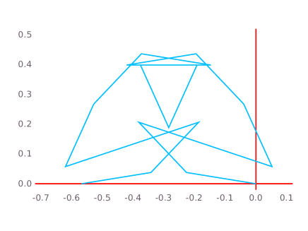
Figure 4. The Kloosterman path $K_{19}(8,1)$

Remark 5.2.

The analogue question for other probabilistic number theory results can also be of interest, and quite deep: if we consider Bagchi’s results ([1, Ch. 5]) concerning vertical translates of the Riemann zeta function restricted to a fixed small circle in the strip $1/2<\mathrm{Re}(s)<1$, then we see that the Riemann Hypothesis for the Riemann zeta function is equivalent to the statement that, for any $t\in\mathbf{R}$, and any such disc, the restriction of $s\mapsto\zeta(s+it)$ belongs to the support of the limiting distribution.

Example 5.3.

We now consider a variant of Kloosterman paths (the Swiss railway clock version) where the partial sums are joined with intervals of length $1/p$, but a pause (of duration $1/p$) is inserted at the “middle point” (the second hand of a Swiss railway clock likewise stops about a second and a half at the beginning of each minute).

This means that we consider again a fixed odd prime $p$ and $(a,b)\in{\mathbf{F}^{\times}_{p}}\times{\mathbf{F}^{\times}_{p}}$, and the polygonal path with $n=p$, $t_{j}=j/p$ and

$$z_{j}=\frac{1}{\sqrt{p}}\sum_{1\leqslant x\leqslant j}e\Bigl{(}\frac{ax+b\bar{x}}{p}\Bigr{)}\quad\text{ for }0\leqslant j\leqslant(p-1)/2,$$

and

$$z_{j}=\frac{1}{\sqrt{p}}\sum_{1\leqslant x\leqslant j-1}e\Bigl{(}\frac{ax+b\bar{x}}{p}\Bigr{)}\quad\text{ for }(p+1)/2\leqslant j\leqslant p,$$

which means in particular that $z_{(p-1)/2}=z_{(p+1)/2}$, representing the pause. Because this pause comes in the middle of the path, we have $f\in\mathcal{{F}}_{0}$.

We get

$$z_{j+1}-z_{j}=\frac{1}{\sqrt{p}}e\Bigl{(}\frac{a(j+1)+b\overline{(j+1)}}{p}\Bigr{)},$$

if $0\leqslant j\leqslant(p-3)/2$, $z_{(p+1)/2}-z_{(p-1)/2}=0$ and

$$z_{j+1}-z_{j}=\frac{1}{\sqrt{p}}e\Bigl{(}\frac{aj+b\bar{\jmath}}{p}\Bigr{)},$$

if $(p+1)/2\leqslant j\leqslant p-1$. Hence the sums $\widetilde{f}(h)$ given by (5.3) become

$$\frac{1}{\sqrt{p}}\sum_{x=0}^{(p-3)/2}e\Bigl{(}\frac{a(x+1)+b\overline{(x+1)}}{p}\Bigr{)}e\Bigl{(}-\frac{h(x+{\textstyle{\frac{1}{2}}})}{p}\Bigr{)}+\frac{1}{\sqrt{p}}\sum_{x=(p+1)/2}^{p-1}e\Bigl{(}\frac{ax+b\bar{x}}{p}\Bigr{)}e\Bigl{(}-\frac{h(x+{\textstyle{\frac{1}{2}}})}{p}\Bigr{)}\\ =\frac{1}{\sqrt{p}}e\Bigl{(}-\frac{h}{2p}\Bigr{)}\sum_{x=1}^{(p-1)/2}e\Bigl{(}\frac{(a-h)x+b\bar{x}}{p}\Bigr{)}+\frac{1}{\sqrt{p}}e\Bigl{(}\frac{h}{2p}\Bigr{)}\sum_{x=(p+1)/2}^{p-1}e\Bigl{(}\frac{(a-h)x+b\bar{x}}{p}\Bigr{)},$$

for all non-zero integers $h$ (it is more convenient here to keep the phase).

These are again close to the Kloosterman sums $\operatorname{Kl}_{2}(a-h,b;p)$, but slightly different. Precisely, let

$$\operatorname{Kl_{2}^{(\cdot)}}(a,b;p)=K_{p}(a,b)(1/2)=\frac{1}{\sqrt{p}}\sum_{x=1}^{(p-1)/2}e\Bigl{(}\frac{ax+b\bar{x}}{p}\Bigr{)}$$

denote the “mezzo del cammin” of the Kloosterman path, so that

$$2\operatorname{Re}(\operatorname{Kl_{2}^{(\cdot)}}(a,b;p))=\operatorname{Kl}_{2}(a,b;p).$$

The sum $\widetilde{f}(h)$ above is then equal to

$$e\Bigl{(}-\frac{h}{2p}\Bigr{)}\operatorname{Kl_{2}^{(\cdot)}}(a-h,b;p)+e\Bigl{(}\frac{h}{2p}\Bigr{)}\overline{\operatorname{Kl_{2}^{(\cdot)}}(a-h,b;p)}=\\ \cos(\pi h/p)\operatorname{Kl}_{2}(a-h,b;p)+2\sin(\pi h/p)\operatorname{Im}(\operatorname{Kl_{2}^{(\cdot)}}(a-h,b;p)).$$

To have $f\in\mathcal{S}$ in this case, we must have

$$\Bigl{|}\frac{\sin(\pi h/p)}{\pi h/p}\widetilde{f}(h)\Bigr{|}\leqslant 2$$

for all $h\not=0$, or (by periodicity of $\widetilde{f}(h)$ and decay of $x\mapsto|\sin(\pi x/p)/(x/p)|$ along arithmetic progressions modulo $p$) when $1\leqslant h\leqslant p-1$. Whether this holds or not depends on the values of the imaginary part of $\operatorname{Kl_{2}^{(\cdot)}}(a-h,b;p)$ as $h$ varies. As in the previous example, it suffices that

(5.6) $$|\widetilde{f}(h)|\leqslant 2$$

for $1\leqslant h\leqslant p-1$.

It follows from [15, Prop. 4.1] that when $p$ is large the random variable $a\mapsto\operatorname{Im}(\operatorname{Kl_{2}^{(\cdot)}}(a,b;p))$ on ${\mathbf{F}^{\times}_{p}}$ takes (rarely but with positive probability) arbitrary large values. This indicates that the property above becomes more difficult to achieve for large $p$. Again, we present numerical illustrations.

Swiss Railway Clock Kloosterman paths $K_{p}(a,1)$ In $\mathcal{S}$ with (5.6) In $\mathcal{S}$ without (5.6) Not in $\mathcal{S}$

c—c—c—c—c $5$ $4$ $0$ $0$

$17$ $14$ $1$ $1$

$23$ $19$ $2$ $1$

$29$ $26$ $2$ $0$

$229$ $204$ $17$ $7$

$541$ $484$ $36$ $20$

$1223$ $1088$ $94$ $40$

$1987$ $1763$ $172$ $51$

$2741$ $2416$ $239$ $85$

$3571$ $3176$ $281$ $113$

The first case of a Swiss Clock Kloosterman path that is not in $\mathcal{S}$ is the one corresponding to $K_{17}(8,1)$, pictured in Figure 5.

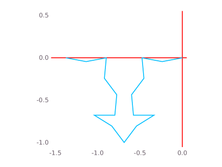
Figure 5. The Kloosterman path $K_{17}(8,1)$

Despite these numbers, we can prove:

Proposition 5.4.

For all $p$ large enough, and all $(a,b)\in{\mathbf{F}^{\times}_{p}}\times{\mathbf{F}^{\times}_{p}}$, we have $f\notin\mathcal{S}$.

Sketch of proof.

By the Weyl criterion, for any fixed $k\geqslant 1$ and any tuple $(b_{1},\ldots,b_{k})$ of non-zero integers, the random variables

$$a\mapsto\Bigl{(}\frac{h}{p},\operatorname{Kl}(a,b_{1};p),\ldots,\operatorname{Kl}(a,b_{k};p)\Bigr{)}\in\mathbf{R}/\mathbf{Z}\times\mathbf{R}^{k}$$

on ${\mathbf{F}_{p}}$ (with uniform probability measure) converge in law as $p\to+\infty$ to independent random variables $(X_{0},\ldots,X_{k})$ where $X_{0}$ is uniformly distributed in $\mathbf{R}/\mathbf{Z}$ and $(X_{1},\ldots,X_{k})$ are independent Sato-Tate random variables. Using the discrete Fourier expansion of $\operatorname{Kl_{2}^{(\cdot)}}(a-h,b;p)$, it follows that, for any fixed $(a,b)$, the random variables

$$h\mapsto\Bigl{(}\frac{h}{p},\operatorname{Kl_{2}^{(\cdot)}}(a-h,b;p)\Bigr{)}\in\mathbf{R}/\mathbf{Z}\times\mathbf{C}$$

on $\{0,\ldots,p-1\}$ (with uniform probability measure) converge in law to $(X_{0},\mathrm{K}(1/2))$ where $X_{0}$ is independent of $\mathrm{K}(1/2)$. Moreover, the convergence is uniform in terms of $(a,b)$.

Therefore, the random variable

$$h\mapsto\frac{\sin(\pi h/p)}{\pi h/p}\widetilde{f}(h)$$

converges in law to

$$Y=2\frac{\sin(\pi X_{0})}{\pi X_{0}}\Bigl{(}\cos(\pi X_{0})\operatorname{Re}(\mathrm{K}(1/2))+\sin(\pi X_{0})\operatorname{Im}(\mathrm{K}(1/2))\Bigr{)}.$$

Since $X_{0}$ and $\mathrm{K}(1/2)$ are independent and the real part of $\mathrm{K}(1/2)$ is between $-1$ and $1$, we have (say)

$$\mathbf{P}(|Y|>2) \geqslant\mathbf{P}(|\operatorname{Im}(K(1/2))|\geqslant 10\text{ and }|X_{0}-1/4|\leqslant 1/10)$$

$$=\mathbf{P}(|\operatorname{Im}(K(1/2))|\geqslant 10)\mathbf{P}(|X_{0}-1/4|\leqslant 1/10)>0$$

since we showed in [15, Prop. 4.1] that $\operatorname{Im}(K(1/2))$ can take arbitrarily large values with positive probability. Hence, for all $p$ large enough, there exists $h$ such that

$$\Bigl{|}\frac{\sin(\pi h/p)}{\pi h/p}\widetilde{f}(h)\Bigr{|}>2.$$

∎

Example 5.5.

Third-time lucky: the next variant of Kloosterman paths will always be realized in $\mathcal{S}$. We now insert two pauses of duration $1/(2p)$ at the beginning and end of the path. Thus $n=p+1$, $t_{0}=0$ and $t_{p+1}=1$, while $t_{i}=(i-{\textstyle{\frac{1}{2}}})/p$ for $1\leqslant i\leqslant p$; moreover $z_{i}$ is given by

$$z_{0}=0,\quad\quad z_{p+1}=\operatorname{Kl}_{2}(a,b;p),$$

and

$$z_{i}=\frac{1}{\sqrt{p}}\sum_{1\leqslant x\leqslant i-1}e\Bigl{(}\frac{ax+b\bar{x}}{p}\Bigr{)}$$

for $1\leqslant i\leqslant p$.

Since the $t_{i}$’s are not all equal, the formula (5.3) does not apply, but we derive from (5.1) that

$$\widehat{f}(h) =-\frac{1}{2i\pi h}\operatorname{Kl}_{2}(a,b;p)+\frac{1}{2i\pi h}\frac{\sin(\pi h/p)}{\pi h/p}\frac{1}{\sqrt{p}}\sum_{x=1}^{p-1}e\Bigl{(}\frac{ax+b\bar{x}}{p}\Bigr{)}e\Bigl{(}-h\frac{x-{\textstyle{\frac{1}{2}}}+{\textstyle{\frac{1}{2}}}}{p}\Bigr{)}$$

$$=-\frac{1}{2i\pi h}\operatorname{Kl}_{2}(a,b;p)+\frac{1}{2i\pi h}\frac{\sin(\pi h/p)}{\pi h/p}\operatorname{Kl}_{2}(a-h,b;p)$$

for all $h\not=0$. By the Weil bound for Kloosterman sums, we conclude that $f\in\mathcal{S}$.

As a consequence of the symmetry properties discussed in Section 3, all paths obtained by applying these symmetries to these modified Kloosterman paths $f$ also belong to $\mathcal{S}$, and therefore can be approximated arbitrarily closely (in the sense of Proposition 1.2) by (actual!) Kloosterman paths. This is quite remarkable, for instance because (at least if $p$ is large enough) neither $-f$ nor $\bar{f}$ is associated to a Kloosterman path (indeed, the pauses show that this would have to be of the same type as $f$ for a Kloosterman path modulo the same prime $p$, and comparing Fourier coefficients, one would need to have either $-\operatorname{Kl}_{2}(a-h,b;p)=\operatorname{Kl}_{2}(c-h,d;p)$ for all $h$ or $\operatorname{Kl}_{2}(a+h,b;p)=\operatorname{Kl}_{2}(c-d,d;p)$ for all $h$; both can be excluded by elementary considerations concerning the Kloosterman sheaf).

Example 5.6.

We proved in [15, Th. 1.3] that the random Fourier series $\mathrm{K}$ is also the limit of the processes $B_{p}$ of partial sums of Birch sums

$$B(a;p)=\frac{1}{\sqrt{p}}\sum_{0\leqslant x\leqslant p-1}e\Bigl{(}\frac{ax+x^{3}}{p}\Bigr{)}$$

where $a\in{\mathbf{F}_{p}}$ is taken uniformly at random. It is then natural to consider these polygonal Birch paths and to ask whether they belong to the support of $\mathrm{K}$. As defined, there is a trivial obstruction: the path $t\mapsto B_{p}(a)(t)$ does not belong to $\mathcal{{F}}_{0}$, because of the initial summand $1/\sqrt{p}$ for $x=0$.

We can alter the path minimally by splitting the summand $1/\sqrt{p}$ in two summands $1/(2\sqrt{p})$ at the beginning and end of the path. The resulting function, which we denote $f$, belongs to $\mathcal{{F}}_{0}$. This means that we consider the polygonal path with $n=p+1$, $t_{i}=(i-{\textstyle{\frac{1}{2}}})/p$ for $1\leqslant i\leqslant p$, and with $z_{i}$ defined by

$$z_{0}=0,\quad\quad z_{p+1}=B(a;p),$$

and

$$z_{i}=\frac{1}{2\sqrt{p}}+\frac{1}{\sqrt{p}}\sum_{1\leqslant j\leqslant i-1}e\Bigl{(}\frac{aj+j^{3}}{p}\Bigr{)}$$

for $1\leqslant i\leqslant p$.

As in the previous example, from (5.1) we get

$$\widehat{f}(h)=-\frac{1}{2i\pi h}B(a;p)+\frac{1}{2i\pi h}\Bigl{\{}\frac{1}{2\sqrt{p}}e\Bigl{(}-\frac{h}{4p}\Bigr{)}\frac{\sin(\pi h/(2p))}{\pi h/(2p)}\\ +\frac{\sin(\pi h/p)}{\pi h/p}\frac{1}{\sqrt{p}}\sum_{x=1}^{p-1}e\Bigl{(}\frac{(a-h)x+x^{3}}{p}\Bigr{)}+\frac{1}{2\sqrt{p}}e\Bigl{(}\frac{h}{4p}\Bigr{)}\frac{\sin(\pi h/(2p))}{\pi h/(2p)}\Bigr{\}}.$$

The inner expression is equal to

$$\frac{1}{\sqrt{p}}\frac{\sin(\pi h/(2p))}{\pi h/(2p)}\cos\Bigl{(}\frac{\pi h}{2p}\Bigr{)}+\frac{\sin(\pi h/p)}{\pi h/p}\Bigl{(}B(a-h;p)-\frac{1}{\sqrt{p}}\Bigr{)}=\frac{\sin(\pi h/p)}{\pi h/p}B(a-h;p).$$

By the Weil bound for Birch sums, we conclude that $f\in\mathcal{S}$.

Example 5.7.

Let $p$ be a prime and $\chi$ a non-trivial Dirichlet character modulo $p$. We consider the polygonal paths interpolating the partial sums of the multiplicative character sum

$$\frac{1}{\sqrt{p}}\sum_{1\leqslant x\leqslant p-1}\chi(x).$$

Let $f$ be the parameterized path where we insert pauses of duration $1/(2p)$ at the beginning and at the end. Note that $f(1)=0$ by orthogonality of characters. As in the previous computations, we get

$$\widehat{f}(h) =\frac{1}{2i\pi h}\frac{\sin(\pi h/p)}{\pi h/p}\frac{1}{\sqrt{p}}\sum_{x=1}^{p-1}\chi(x)e\Bigl{(}-h\frac{x-{\textstyle{\frac{1}{2}}}+{\textstyle{\frac{1}{2}}}}{p}\Bigr{)}$$

$$=\frac{1}{2i\pi h}\frac{\sin(\pi h/p)}{\pi h/p}\chi(-1)\tau(\chi)\overline{\chi(h)},$$

where

$$\tau(\chi)=\frac{1}{\sqrt{p}}\sum_{1\leqslant x\leqslant p-1}\chi(x)e\Bigl{(}\frac{x}{p}\Bigr{)}$$

is the normalized Gauss sum associated to $\chi$ (note that $\chi(h)=0$ if $p\mid h$). Since $|\tau(\chi)|=1$, it follows that $|\widehat{f}(h)|\leqslant 1$. However, the Fourier coefficients are only in $i\mathbf{R}$ (i.e., $f\in\mathcal{{F}}_{0}$) if $p\equiv 1\,(\mathrm{mod}\,{4})$ and $\chi$ is a real character. In other words, Kloosterman sums can perfectly mimic the character sums associated to the Legendre symbol modulo such primes. (Note that in this case, the function $f$ is real-valued).

Note that character sums as above have been very extensively studied from many points of view, because of their importance in many problems of analytic number theory, for instance in the theory of Dirichlet $L$-functions. We refer for instance to the works [9, 4, 5] of Bober, Goldmakher, Granville, Koukoulopoulos and Soundararajan (in various combinations). It should be possible (and interesting) to study the support of the limiting distribution of these character paths, but this will be very different from $\mathcal{S}$. Indeed, one can expect (see [5]) that the support in this case would be continuous functions with totally multiplicative Fourier coefficients. For instance, one can expect that $0$ does not belong to the support in that case.

Example 5.8.

More generally, consider a prime $p$ and the polygonal path $f$ associated to the partial sums of any exponential sum

$$\frac{1}{\sqrt{p}}\sum_{1\leqslant x\leqslant p}\chi(g_{1}(x))e\Bigl{(}\frac{g_{2}(x)}{p}\Bigr{)},$$

where $\chi$ is a Dirichlet character modulo $p$, and $g_{1}$ and $g_{2}$ are polynomials in $\mathbf{Z}[X]$ (with $g_{2}$ non-constant). After suitable tweaks, the Fourier coefficients become

$$\widetilde{f}(h)=\frac{\sin(\pi h/p)}{\pi h/p}\frac{1}{\sqrt{p}}\sum_{1\leqslant x\leqslant p}\chi(g_{1}(x))e\Bigl{(}\frac{g_{2}(x)-xh}{p}\Bigr{)}.$$

Assuming $f\in\mathcal{{F}}_{0}$, and under suitable restrictions, we may expect that $f\in\mathcal{S}$ only if the geometric monodromy group of the Fourier transform of the rank $1$ sheaf with trace function the summand

$$x\mapsto\chi(g_{1}(x))e\Bigl{(}\frac{g_{2}(x)}{p}\Bigr{)}$$

has rank $r$ at most $2$ (otherwise, Deligne’s equidistribution theorem will lead in most cases to the existence of $h$ such that $0\leqslant h\leqslant p-1$ and $|\widetilde{f}(h)|\geqslant(r-1/2)>2$).

Example 5.9.

A natural question is whether $\mathcal{S}$ contains a space-filling curve. Among the classical examples of such curves, the Hilbert curve [23, Ch. 2] has a sequence of quite simple polygonal approximations $f_{n}$ for $n\geqslant 1$ that belong to $\mathcal{{F}}_{0}$ (see [23, p. 14]). We have in Figure 6 the plots of the second, third and fourth such approximations (note that there are many backtrackings, so this is a case where the plot doesn’t give a clear idea of the path followed).

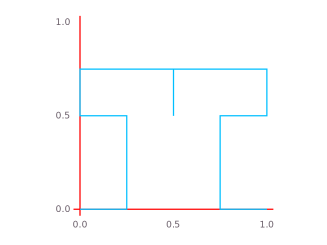
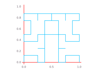
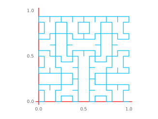
Figure 6. Approximations of the Hilbert function

The function $f_{n}$ is a polygonal path composed of $4^{n}$ segments of length $2^{-n}$. One checks that the Fourier coefficients are given by

$$\widetilde{f}_{n}(h)=\frac{1}{2^{n}}\sum_{j=0}^{4^{n}-1}i^{\delta_{n}(j)}e\Bigl{(}-\frac{h(j+1/2)}{4^{n}}\Bigr{)},$$

for $h\not=0$, where the exponents $\delta_{n}(j)$ (in $\mathbf{Z}/4\mathbf{Z}$) are determined inductively by

$$\delta_{1}(0)=1,\quad\delta_{1}(1)=\delta_{1}(2)=0,\quad\delta_{1}(3)=3,$$

and

$$\delta_{n+1}(4j)=1-\delta_{n}(j),\quad\delta_{n+1}(4j+1)=\delta_{n+1}(4j+2)=\delta_{n}(j),\quad\delta_{n+1}(4j+3)=3-\delta_{n}(j)$$

for $n\geqslant 1$ and $0\leqslant j\leqslant 4^{n}-1$. The requirement for $f_{n}$ to belong to $\mathcal{S}$ is satisfied when these sums exhibit precisely the analogue of the Weil bounds for $1\leqslant h\leqslant 4^{n}-1$. This may or may not happen, and it turns out (numerically) that the first three approximations are in $\mathcal{S}$, but not the fourth.

6. Changing the parameterization

When we display the picture of a Kloosterman path, we are really only seeing the image of the corresponding function from $[0,1]$ to $\mathbf{C}$. Although it is not really an arithmetic question anymore, it seems fairly natural to ask which subsets of $\mathbf{C}$ are really going to appear. This may be interpreted in different ways: (1) given a function $f$ in $\mathcal{{F}}_{0}$, but not in $\mathcal{S}$, when does there exist a change of variable $\varphi\colon[0,1]\to[0,1]$ such that $f\circ\varphi$ belongs to $\mathcal{S}$? (2) given a compact subset $X\subset\mathbf{C}$, when does there exist an element $f\in\mathcal{S}$ such that $X=f([0,1])$?

A priori, these questions might be quite different. However, we first show that the second essentially reduces to the first. Precisely, we have a topological characterization of images of functions in $\mathcal{{F}}_{0}$.

Proposition 6.1.

Let $X\subset\mathbf{C}$ be a compact subset. The following conditions are equivalent:

1. There exists $f\in\mathcal{{F}}_{0}$ such that $X$ is the image of $f$.

2. We have $0\in X$, there exists a real number $\alpha$ such that $X$ is symmetric with respect to the line $\operatorname{Re}(z)=\alpha$, and there exists a continuous function $f\in C([0,1])$ such that $X=f([0,1])$.

3. We have $0\in X$, there exists a real number $\alpha$ such that $X$ is symmetric with respect to the line $\operatorname{Re}(z)=\alpha$, and $X$ is connected and locally connected.

Proof.

It is immediate that (1) implies (2). Conversely, assume that (2) holds and let $f$ be a continuous function such that $f([0,1])=X$. Let $r\colon\mathbf{C}\to\mathbf{C}$ be the symmetry along the line $\operatorname{Re}(z)=\alpha$, so that $X=r(X)$. By assumption, there exist $s_{0}\in[0,1]$ and $s_{1}\in[0,1]$ be such that $f(s_{0})=0$ and $f(s_{1})=r(0)=2\alpha$. Up to replacing $f$ by $t\mapsto f(1-t)$, we may assume that $s_{0}\leqslant s_{1}$.

Let $T$ be the set of all $t\in[0,1]$ such that $t\geqslant s_{0}$ and $\operatorname{Re}(f(t))=\alpha$. This set is closed and it is non-empty (because the image of the continuous real-valued function $\operatorname{Re}(f)$ contains $0=f(s_{0})$ and $r(0)=2\alpha=f(s_{1})$ by assumption, and $s_{1}\geqslant s_{0}$). Let $t_{0}=\max T$ and $Y=f([0,t_{0}])\cup r(f([0,t_{0}]))$. We claim that $X=Y$. Indeed, suppose some $x\in X$ is not in $Y$. Then we also have $r(x)\notin Y$. Hence we can write $x=f(t_{1})$ with $t_{1}>t_{0}$ and $r(x)=f(t_{2})$ with $t_{2}>t_{0}$. Then

$$\alpha=\frac{1}{2}(\operatorname{Re}(f(t_{2}))+\operatorname{Re}(f(t_{1})),$$

so $\alpha$ is in the interval between $\operatorname{Re}(f(t_{1}))$ and $\operatorname{Re}(f(t_{2}))$. By continuity, there exists $s$ between $t_{1}$ and $t_{2}$ with $\operatorname{Re}(f(s))=\alpha$, contradicting the maximality of $t_{0}$.

Now define

$$g(t)=\begin{cases}f(s_{0}(1-8t))&\text{ if }0\leqslant t\leqslant 1/8\\ f(2s_{0}(t-1/8))&\text{ if }1/8\leqslant t\leqslant 1/4\\ f(s_{0}+4(t_{0}-s_{0})(t-1/4))&\text{ if }1/4\leqslant t\leqslant 1/2\end{cases}$$

and $g(t)=r(g(1-t))=2\alpha-\overline{g(1-t)}$ if $1/2<t\leqslant 1$ (in other words, $g(t)$ covers the path of $f$ from $0=f(s_{0})$ to $f(0)$ for $t\in[0,1/8]$, then covers it backwards from $t=1/8$ to $t=1/4$, then follows the path over $[1/4,1/2]$ from $0$ to $f(t_{0})$, and then proceeds by reflection).

We have $g(0)=0$ and $g$ is continuous (because $\operatorname{Re}(g(1/2))=\operatorname{Re}(f(t_{0}))=\alpha$), hence $g\in\mathcal{{F}}_{0}$ by construction. The image of $g$ is contained in $X$; it contains $f([0,t_{0}])$ and its reflection, so its image is $X$. This proves (1) for the set $X$.

To prove that (2) and (3) are equivalent, we simply need to invoke the Hahn-Mazurkiewicz Theorem (see, e.g., [23, Th. 6.8] or [6, TA, III, p. 272, th. 1]): a non-empty compact subset $X\subset\mathbf{C}$ is the image of a continuous function $f\colon[0,1]\to\mathbf{C}$ if and only if $X$ is connected and locally connected. ∎

Because of this proposition, it is natural to concentrate on the change of variable problem. Here a subtlety is whether we wish to have an invertible reparameterization or not: if $\varphi\colon[0,1]\to[0,1]$ is merely surjective, the image of $f\circ\varphi$ is the same as that of $f$. However, we consider here only transformations $\varphi$ that are homeomorphisms. In fact, let us say that an increasing homeomorphism $\varphi$ of $[0,1]$ such that $\varphi(1-t)=1-\varphi(t)$ is a symmetric homeomorphism. We then have $f\circ\varphi\in\mathcal{{F}}_{0}$ for all $f\in\mathcal{{F}}_{0}$. The question is: for a given $f\in\mathcal{{F}}_{0}$, does there exist a symmetric homeomorphism $\varphi$ such that $f\circ\varphi\in\mathcal{S}$?

To prove our result for real-valued functions in Proposition 1.4, we will use a variant of a result of Sahakian [22, Cor. 2].

Recall that the Faber-Schauder functions $\Lambda_{m,j}$ on $[0,1]$ are defined for $m\geqslant 0$ and $1\leqslant j\leqslant 2^{m}$ by the following conditions:

• The support of $\Lambda_{m,j}$ is the dyadic interval

  $$\Bigl{[}\frac{j-1}{2^{m}},\frac{j}{2^{m}}\Bigr{]},$$

  of length $2^{-m}$,

• We have $\Lambda_{m,j}((2j-1)2^{-m-1})=1$,

• The function $\Lambda_{m,j}$ is affine on the two intervals

  $$\Bigl{[}\frac{j-1}{2^{m}},\frac{2j-1}{2^{m+1}}\Bigr{]},\quad\quad\Bigl{[}\frac{2j-1}{2^{m+1}},\frac{j}{2^{m}}\Bigr{]}.$$

Any continuous function $f$ on $[0,1]$ has a uniformly convergent Faber-Schauder series expansion

$$f(t)=\beta(0)+\beta(1)t+\sum_{m\geqslant 0}\sum_{j=1}^{2^{m}}\beta(m,j)\Lambda_{m,j}(t),$$

with coefficients

$$\beta(0)=f(1),\quad\quad\beta(1)=f(1)-f(0),$$

and

(6.1) $$\beta(m,j)=f\Bigl{(}\frac{2j-1}{2^{m+1}}\Bigr{)}-\frac{1}{2}\Bigl{(}f\Bigl{(}\frac{j-1}{2^{m}}\Bigr{)}+f\Bigl{(}\frac{j}{2^{m}}\Bigr{)}\Bigr{)}$$

(see, e.g., [13, Ch. VI] for these facts). The function $f$ is $1$-periodic if and only if $\beta(1)=0$.

Theorem 6.2 (Sahakian).

Let $g\colon[0,1]\to\mathbf{R}$ be a real-valued continuous function with $g(0)=0$. Let $\varepsilon>0$ be any fixed positive real number.

(1) There exists an increasing homeomorphism $\varphi\colon[0,1]\to[0,1]$ such that the Fourier coefficients of the function $u(g\circ\varphi)=g\circ\varphi-g(1)t$ satisfy

$$|\widehat{u(g\circ\varphi)}(h)|\leqslant\frac{\varepsilon}{|h|}$$

for all $h\not=0$.

(2) If the function $g$ satisfies $g(t)+g(1-t)=g(1)$ for all $t$, then we may assume that $\varphi$ is symmetric.

We emphasize that the function $g$ is real-valued; it does not seem to be known whether the statement (1) holds for a complex-valued function $g$. The issue in the proof in [22] is the essential use of the intermediate value theorem.

Sketch of proof.

Below, we will say that a continuous function $g\colon[0,1]\to\mathbf{C}$ is $1$-periodic if $g(0)=g(1)$, which means that the periodic extension of $g$ to $\mathbf{R}$ is continuous.

The result requires only very minor changes in Sahakian’s argument, which does not address exactly this type of uniform “numerical” bounds, but asymptotic statements like $|\widehat{(g\circ\varphi)}(h)|=o(|h|^{-1})$ as $|h|\to+\infty$ when $g$ is $1$-periodic.

For any continuous $1$-periodic function $f$ on $[0,1]$, extended to $\mathbf{R}$ by periodicity, define

$$\omega_{f}(\delta)=\sup_{0<\alpha\leqslant\delta}\int_{0}^{1}|f(x+\alpha)+f(x-\alpha)-2f(x)|dx.$$

A classical elementary argument (compare [25, II.4]) shows that for a $1$-periodic function $f$, we have

(6.2) $$|\widehat{f}(h)|\leqslant\frac{1}{4}\omega_{f}\Bigl{(}\frac{1}{|h|}\Bigr{)}$$

for all $h\not=0$. It is also elementary that there exists $C>0$ such that

$$\omega_{\Lambda_{m,j}}(\delta)\leqslant C\min(2^{m}\delta^{2},2^{-m})$$

for all $m$ and $j$.

By [22, Lemma 1], applied to the continuous real-valued function $t\mapsto g(2\pi t)$ on $[0,2\pi]$, there exists a homeomorphism $\varphi$ such that, for any $m\geqslant 0$, the coefficients $\beta(m,j)$ of the Faber-Schauder expansion of $g\circ\varphi$ vanish for all but at most one index $j_{m}$, and moreover, we have

$$|\beta(m,j_{m})|<\frac{\varepsilon}{C}.$$

Note that the text of [22] might suggest that the lemma is stated for $1$-periodic functions, but the proof is in fact written for arbitrary continuous functions (as it must, since it proceeds by an inductive argument from $[0,1]$ to dyadic sub-intervals, and any periodicity assumption in the construction would be lost after the first induction step).

Let $\gamma_{m}=\beta(m,j_{m})$ and $\Phi_{m}=\Lambda_{m,j_{m}}$. Since $g(1)=g(\varphi(1))$, we have the series expansion

$$u(g\circ\varphi)(t)=(g\circ\varphi)(t)-g(1)t=\sum_{m\geqslant 0}\gamma_{m}\Phi_{m}(t),$$

uniformly for $t\in[0,1]$ and hence, using the subadditivity of $f\mapsto\omega_{f}$, we get

$$\omega_{u(g\circ\varphi)}(\delta)\leqslant\varepsilon\sum_{m\geqslant 0}\min(2^{m}\delta^{2},2^{-m})\leqslant 4\varepsilon\delta.$$

By (6.2), we get

$$|(\widehat{u(g\circ\varphi)})(h)|\leqslant\frac{\varepsilon}{|h|}.$$

for $h\not=0$, which proves the first statement.

Consider now the case when the condition $g(t)+g(1-t)=g(1)$ holds. We then apply the previous argument (properly scaled) to the restriction of $g$ to $[0,1/2]$, obtaining an increasing homeomorphism $\psi$ of $[0,1/2]$ such that

(6.3) $$(g\circ\psi)(t)-2g(1/2)t=(g\circ\psi)(t)-g(1)t=\sum_{m\geqslant 1}\gamma_{m}\Phi_{m}(t)$$

for $0\leqslant t\leqslant 1/2$ where $|\gamma_{m}|\leqslant\varepsilon C^{-1}$ and $\Phi_{m}$ is a Faber-Schauder function associated to an interval of length $2^{-m}$ of $[0,1/2]$.

We define $\varphi\colon[0,1]\to[0,1]$ so that $\varphi$ coincides with $\psi$ on $[0,1/2]$ and $\varphi(1-t)=1-\varphi(t)$ for $0\leqslant t\leqslant 1/2$. Then $\varphi$ is a symmetric homeomorphism of $[0,1]$. Because of the symmetry of $g$ and (6.3), we have for $1/2\leqslant t\leqslant 1$ the formula

$$(g\circ\varphi)(t)=g(1)-g(\varphi(1-t)) =g(1)-(1-t)g(1)-\sum_{m\geqslant 1}\gamma_{m}\Phi_{m}(1-t)$$

$$=g(1)t-\sum_{m\geqslant 1}\gamma_{m}\Phi_{m}(1-t).$$

Since the supports are disjoint, we can therefore write

$$u(g\circ\varphi)(t)=(g\circ\varphi)(t)-g(1)t=\sum_{m\geqslant 1}\gamma_{m}\Phi_{m}(t)-\sum_{m\geqslant 1}\gamma_{m}\Phi_{m}(1-t)$$

for all $t\in[0,1]$. Now we evaluate the Fourier coefficients as before. ∎

We can now prove Proposition 1.4.

Proof of Proposition 1.4.

Let $f$ be a real-valued function $f\in\mathcal{{F}}_{0}$ with $|f(1)|\leqslant 2$. Theorem 1.1 and Theorem 6.2 (2) applied to $f$ (which satisfies $f(t)+f(1-t)=f(1)$ since it is real-valued) with $\varepsilon=1/\pi$ imply the existence of the desired reparameterization. ∎

Remark 6.3.

(1) The prototypical statement of “improvement” of convergence of a Fourier series by change of variable is the Bohr-Pál Theorem (see, e.g., [25, Th. VII.10.18]), which gives for any $1$-periodic continuous real-valued function $f$ a homeomorphism $\varphi$ of $[0,1]$ such that the Fourier $f\circ\varphi$ converges uniformly on $[0,1]$. The extension to complex-valued functions was obtained by Kahane and Katznelson [12].

(2) It seems that the problem of obtaining the bound $\widehat{f\circ\varphi}(h)=O(|h|^{-1})$ for a complex-valued $1$-periodic function $f\in C([0,1])$ is quite delicate. For instance, let $W_{2}^{1/2}$ be the Banach space of integrable functions $f$ on $[0,1]$ such that

$$\sum_{h\in\mathbf{Z}}|h||\widehat{g}(h)|^{2}<+\infty.$$

Let $f_{1}$ be a real-valued $1$-periodic function in $C([0,1])$. Lebedev [17, Th. 4] proves that if $f_{1}$ has the property that, for any $f\in C([0,1])$ with real part $f_{1}$, there exists an homeomorphism $\varphi$ such that both $f_{1}\circ\varphi=\operatorname{Re}(f)\circ\varphi$ and $\operatorname{Im}(f)\circ\varphi$ belong to $W_{2}^{1/2}$, then $f_{1}$ is of bounded variation (and indeed, the converse is true).

(3) Note that in any reparameterization $f\circ\varphi$ of $f\in\mathcal{{F}}_{0}$ with $\varphi$ symmetric, the coefficient $\beta(0,1)$ of the Faber-Schauder function $\Lambda_{0,1}$ is unchanged: because $\varphi(1/2)=1/2$, it is

$$\beta(0,1)=f\Bigl{(}\frac{1}{2}\Bigr{)}-\frac{1}{2}(f(0)+f(1))=\operatorname{Im}(f({\textstyle{\frac{1}{2}}})).$$

In particular, one cannot hope to reparameterize all functions with $f(1/2)\notin\mathbf{R}$ using information on the Faber-Schauder expansion of $f\circ\varphi$ and individual estimates for each Faber-Schauder function that is involved.

References

- [1] B. Bagchi: Statistical behaviour and universality properties of the Riemann zeta function and other allied Dirichlet series, PhD thesis, Indian Statistical Institute, Kolkata, 1981; available at library.isical.ac.in:8080/jspui/bitstream/10263/4256/1/
- [2] P. T. Bateman and S. Chowla: Some special trigonometrical series related to the distribution of prime numbers, Journal London Math. Soc. 38 (1963), 372–374.
- [3] P. Billingsley: Convergence of probability measures, 2nd edition, Wiley, 1999.
- [4] J.W. Bober and L. Goldmakher: The distribution of the maximum of character sums, Mathematika 59 (2013), 427–442.
- [5] J.W. Bober, L. Goldmakher, A. Granville and D. Koukoulopoulos: The frequency and the structure of large character sums, Journal European Math. Soc., to appear arXiv:1410.8189.
- [6] N. Bourbaki: Éléments de mathématique.
- [7] J.J. Duistermaat: Selfsimilarity of ’Riemann’s non-differentiable function’, Nieuw Arch. Wisk. (4) 9 (1991), 303–337.
- [8] I.S. Gradshteyn and I.M. Ryzhkik: Tables of integrals, series and products, 5th ed. (edited by A. Jeffrey), Academic Press (1994).
- [9] A. Granville and K. Soundararajan: Large character sums: pretentious characters and the Pólya-Vinogradov theorem, Journal of the AMS 20 (2007), 357– 384.
- [10] J. Bezanson, A. Edelman, S. Karpinski, V. B. Shah: Julia: A fresh approach to numerical computing, SIAM Review (2017), 59:65–98, doi:10.1137/141000671.
- [11] H. Iwaniec and E. Kowalski: Analytic number theory, Colloquium Publ. 53, A.M.S (2004).
- [12] J-P. Kahane and Y. Katznelson: Séries de Fourier des fonctions bornées, with an appendix by L. Carleson, Birkhäuser (1983), 395–413,
- [13] B.S. Kashin and A.A. Sahakian: Orthogonal series, Translations of mathematical monographs 75, A.M.S. (1989).
- [14] E. Kowalski: Arithmetic Randonnée: an introduction to probabilistic number theory, lectures notes, www.math.ethz.ch/~kowalski/probabilistic-number-theory.pdf
- [15] E. Kowalski and W. Sawin: Kloosterman paths and the shape of exponential sums, Compositio Math. 152 (2016), 1489–1516.
- [16] J. Lagarias: The Takagi function and its properties, in Functions and Number Theory and Their Probabilistic Aspects, RIMS Kokyuroku Bessatsu B34, Aug. 2012, pp. 153–189.
- [17] V. Lebedev: Change of variable and the rapidity of decrease of Fourier coefficients, Matematicheskiĭ Sbornik, 181:8 (1990), 1099–1113 (Russian), English translation arXiv:1508.06673v2.
- [18] A.M. Olevskiĭ: Modifications of functions and Fourier series, Uspekhi Mat. Nauk, 40:3 (1985), 157–193 (Russian); English translation in Russian Math. Surveys, 40:3 (1985), 181–224.
- [19] J. Pach and C.A. Rogers: Partly convex Peano curves, Bull. London Math. Soc. 15 (1983), 321–328.
- [20] PARI/GP, The PARI Group, PARI/GP version 2.8.0, Univ. Bordeaux, 2016, pari.math.u-bordeaux.fr/.
- [21] G. Ricotta and E. Royer: Kloosterman paths of prime power moduli, preprint (2016).
- [22] A.A. Sahakian: Integral moduli of smoothness and the Fourier coefficients of the composition of function, Mat. Sb. 110 (1979), 597–608; English translation, Math. USSR Sbornik 38 (1981), 549–561, iopscience.iop.org/0025-5734/38/4/A07.
- [23] H. Sagan: Space-filling curves, Universitext, Springer 1994.
- [24] G. N. Watson: A treatise on the theory of Bessel functions, 2nd ed., Cambridge Math. Library, Cambridge Univ. Press (1996).
- [25] A. Zygmund: Trigonometric series, vol. 1 and 2 combined, Cambridge Math. Library, Cambridge Univ. Press (2002).