Thermodynamic formalism and
integral means spectrum of logarithmic tracts
for transcendental entire functions

Abstract.

We provide an entirely new approach to the theory of thermodynamic formalism for entire functions of bounded type. The key point is that we introduce an integral means spectrum for logarithmic tracts which takes care of the fractal behavior of the boundary of the tract near infinity. It turns out that this spectrum behaves well as soon as the tracts have some sufficiently nice geometry which, for example, is the case for quasidisk, John or Hölder tracts. In these cases we get a good control of the corresponding transfer operators, leading to full thermodynamic formalism along with its applications such as exponential decay of correlations, central limit theorem and a Bowen’s formula for the Hausdorff dimension of radial Julia sets.

This approach covers all entire functions for which thermodynamic formalism has been so far established and goes far beyond. It applies in particular to every hyperbolic function from any Eremenko-Lyubich analytic family of Speiser class $\mathcal{S}$ provided this family contains at least one function with Hölder tracts. The latter is, for example, the case if the family contains a Poincaré linearizer.

1. Introduction

The dynamics of a holomorphic function heavily depends on the behavior of the singular set. The singular set $S(f)$ of an entire function $f:{\mathbb{C}}\to{\mathbb{C}}$ is the closure of the set of critical values and finite asymptotic values of $f$. Eremenko-Lyubich [15] introduced and studied class $\mathcal{B}$ consisting of all entire functions with bounded singular sets. It has as a subclass Speiser class $\mathcal{S}$ consisting of entire functions with finite singular sets. In this paper we develop the full theory of thermodynamic formalism for a large collection of entire functions in Eremenko-Lyubich class $\mathcal{B}$.

When developing the thermodynamic formalism for transcendental functions, one encounters immediately two major difficulties: one has to deal with the essential singularity at infinity and to check whether the transfer operator, which is given by an infinite series, is well defined, i.e. converges, and has sufficiently good properties.

The first work on thermodynamic formalism for transcendental functions is due to Barański [1] who considered the tangent family. Other specific, mainly periodic, functions have been treated in the sequel, see for example [20], [43] and [44]. The first and, up to now, the only unified approach appeared in [24] and in [25]. These papers deal with a large class of functions that satisfy a condition on the derivative called the balanced growth condition. The key point there was to employ Nevanlinna Theory and to make a judicious choice of Riemannian metric. Here we keep this choice of metric but then we proceed totally differently avoiding any use of Nevanlinna Theory. By introducing the integral means spectrum for logarithmic tracts we built the theory of thermodynamic formalism for many other entire functions from class $\mathcal{B}$.

The main object of this paper is to show that the transfer operator behaves well depending on the geometry of the logarithmic tracts over infinity. Consider $f\in\mathcal{B}$ and suppose that the bounded set $S(f)$ is contained in the unit disk. Then, the components $\Omega_{j}$ of $f^{-1}(\{|z|>1\})$ are the tracts, in fact logarithmic tracts of $f$ over infinity. We assume that there are only finitely many of them: see the definition of class $\mathcal{D}$ in the next section.

Let us consider here in this introduction the case where $f^{-1}(\{|z|>1\})$ consists of only one tract $\Omega$. Then, $f_{|\Omega}$ has the particular form $f=e^{\tau},$ with $\tau$ a conformal map from $\Omega$ onto the half plane $\mathcal{H}=\{\Re z>0\}$ such that

(1.1) $$\varphi:=\tau^{-1}:\mathcal{H}\to\Omega$$

extends continuously to infinity [15]. Although $\partial\Omega$ is an analytic curve, near infinity it often resembles more and more a fractal curve. Typically, going to infinity on $\partial\Omega$ is like considering Green lines that are closer and closer to the boundary of possibly fractal domains. To make this precise, consider the rectangles

(1.2) $$Q_{T}:=\big{\{}\xi\in{\mathbb{C}}:0<\Re\xi<4T\ \ {\rm and}\ \ -4T<\Im\xi<4T\big{\}}$$

and then the domains

$$\Omega_{T}:=\varphi(Q_{T})\;,\ \ T\geq 1\,.$$

The domains $\Omega_{T}$ form natural exhaustions of $\Omega$ and the fractality near infinity of $\partial\Omega$ can be observed by considering $\Omega_{T}$ rescaled by the factors $1/|\varphi(T)|$ as $T\to\infty$.

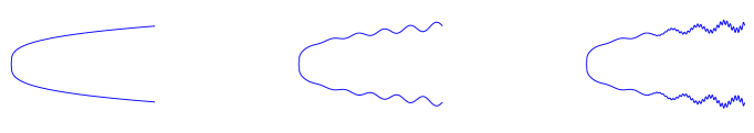
Figure 1. Example of $\frac{\Omega_{T}}{|\varphi(T)|}$ for $T=1$, $T=5$ and $T=20$.

The corresponding rescaled map is given by the formula

$$\varphi_{T}(z):=\frac{1}{|\varphi(T)|}\varphi(T(z))$$

and one can consider the integral means

$$\beta_{\varphi_{T}}(r,t):=\frac{\log\int_{1\leq|y|\leq 2}|\varphi_{T}^{\prime}(r+iy)|^{t}dy}{\log 1/r}\,.$$

Starting from this formula we naturally assign to the tract $\Omega$ an integral means spectrum $\beta_{\infty}$ which measures the fractal behavior of the tract at infinity. As in the classical setting, the important function will be the convex one:

$$b_{\infty}(t):=\beta_{\infty}(t)-t+1\quad,\quad t\in{\mathbb{R}}\,.$$

This function always has a smallest zero $\Theta_{f}>0$ and, in the good cases, $b_{\infty}$ has a unique zero and is negative in $(\Theta_{f},\infty)$. In this latter case, we will say that the function $f$ has negative spectrum.

It will become transparent in Proposition 4.3 that there is a strong relation between the transfer operator, on whose properties the thermodynamic formalisms relies, and the integral means spectrum and we will derive from this that the negative spectrum property implies good behavior of this operator. Negative spectrum turns out to be a very general condition which holds as soon as the tracts have some nice geometry such as the Hölder tract property which essentially means that the domains $\Omega_{T}$ are uniformly Hölder, see Definition 5.3 for the precise definition. For example, if the tract itself $\Omega$ is a quasidisk then it is a Hölder tract.

Proposition 1.1.

Let $f\in\mathcal{B}$ be an entire function having finitely many tracts. If the tracts are Hölder then $f$ has negative spectrum.

Throughout the paper we will primarily work with functions of so called disjoint type, which is a particular form of hyperbolicity; we will provide its precise definition in the sequel. We would however like to note that for functions within class $\mathcal{S}$, by using standard bounded distortion arguments, our results carry over to all hyperbolic functions (see Section 10.1) and not merely those of disjoint type. Class $\mathcal{D}$, for which most of our main results will be formulated and proved, essentially consists in disjoint type functions of class $\mathcal{B}$ having finitely many tracts, see Definition 2.1.

Theorem 1.2.

Let $f\in\mathcal{D}$ be a function having negative spectrum and let $\Theta_{f}\in]0,2]$ be the smallest zero of $b_{\infty}$. Then, the following holds:

• For every $t>\Theta_{f}$, the whole thermodynamic formalism, along with its all usual consequences holds: the Perron-Frobenius-Ruelle Theorem, the Spectral Gap property along with its applications: Exponential Mixing, Exponential Decay of Correlations and Central Limit Theorem (see Section 8).

• For every $t<\Theta_{f}$, the series defining the transfer operator ${\mathcal{L}}_{t}$ (see (4.3)) is divergent.

Therefore, thermodynamic formalism is crystal clear for functions in class $\mathcal{D}$ with negative spectrum. The proof is based on Theorem 4.1 which is valid for all functions in class $\mathcal{B}$ without any further assumptions.

There is a very general result of approximating a model function by entire functions due to Bishop [9, 10]. His work is motivated by earlier results of Rempe-Gillen [39]. We show in Proposition 6.3 that the Hölder tract property is preserved when passing from the model to the approximating entire function. In fact, as Lemma 6.1 demonstrates, the Hölder tract property is a quasiconformal invariant. This has a second important application: for entire functions of class $\mathcal{S}$ the Hölder tract property is in fact a property of an analytic family of functions and not only of a single function. More precisely, if $g\in\mathcal{S}$ then Eremenko-Lyubich [15] naturally associated to $g$ an analytic family of entire functions $\mathcal{M}_{g}\subset\mathcal{S}$. Proposition 10.1 states that every function of $\mathcal{M}_{g}$ has Hölder tracts if a function, for example $g$, has. A concrete application of all of this is the following.

Theorem 1.3.

Let $g\in\mathcal{S}$ be any function having finitely many tracts over infinity and assume that they are Hölder. Then every function $f\in\mathcal{M}_{g}$ has negative spectrum and the thermodynamic formalism holds for every hyperbolic map from $\mathcal{M}_{g}$.

We also study a particular family of entire functions called Poincaré functions studied previously in [12, 29, 14] among others. If $p:{\hat{\mathbb{C}}}\to{\hat{\mathbb{C}}}$ is a polynomial and if $z_{0}\in\mathcal{J}_{p}$ is a repelling fixed point of $p$ then there exists an entire function $f:{\mathbb{C}}\to{\mathbb{C}}$ such that

(1.3) $$f(p^{\prime}(z_{0})z)=p(f(z))\quad\text{for all $z\in{\mathbb{C}}$.}$$

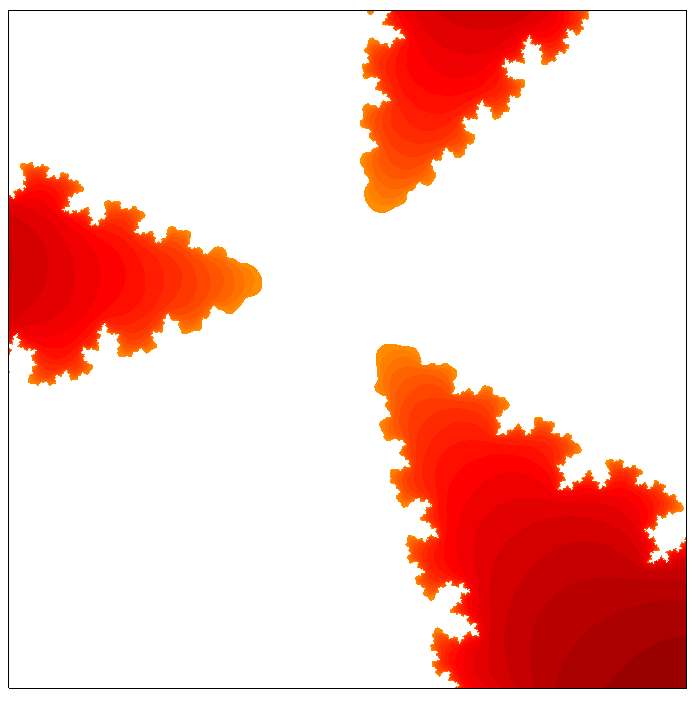
Figure 2. Three fractal and Hölder tracts from a linearizer of Douady’s Rabbit.

For all entire functions $f$ that obey such a particular linearizing functional equation such that the involved polynomial $p$ has a connected Julia set we show, by a direct calculation in Theorem 7.8, that the transfer operator behaves well. But not all of them have negative spectrum. Based on the work of Graczyk, Przytycki, Rivera-Letelier and Smirnov [17, 34], we show that Poincaré functions have Hölder tracts if and only if the corresponding linearizing polynomial is topological Collet-Eckmann (TCE). In addition, such a linearizer is in $\mathcal{S}$ if and only if the polynomial is post-critically finite (thus TCE). Therefore, such functions can be taken as generating function of the analytic family in Theorem 1.3. They are particularly intriguing since it follows from Zdunik’s Theorem 7.7 in [46] that the tracts of Poincaré functions are fractals except for the case of polynomials of the form $z\mapsto z^{d}$, $d\geq 2$, or Tchebychev ones.

Corollary 1.4.

Let $g\in\mathcal{S}$ be a Poincaré function of a polynomial having connected Julia set. Then every function $f\in\mathcal{M}_{g}$ has negative spectrum and the thermodynamic formalism holds for every hyperbolic map from $\mathcal{M}_{g}$.

This also leads to geometric applications provided that the topological pressure, as defined in Section 9, has a zero $h>\Theta_{f}$. The following result completes the picture on various Bowen’s Formulas (see [24] but especially [4] which contains a very general version of it).

Theorem 1.5 (Bowen’s Formula).

Let $f\in\mathcal{D}$ have negative spectrum and be such that the topological pressure $\text{{\rm P}}(t)$ has a zero $h>\Theta_{f}$. Then, the hyperbolic dimension $\text{{\rm HypDim}}(f)$ of $f$ is equal to the unique zero $h>\Theta_{f}$ of the topological pressure.

Here is an other concrete application which is based on the previous formula.

Theorem 1.6 (Real analyticity of hyperbolic dimension).

Let $p:{\hat{\mathbb{C}}}\to{\hat{\mathbb{C}}}$ be a hyperbolic polynomial with connected Julia set, let $z_{0}\in\mathcal{J}_{p}$ be a repelling fixed point of $p$ and let $f:{\mathbb{C}}\to{\mathbb{C}}$ be an entire function such that (1.3) holds. Let the entire functions $f_{\kappa}$ be given by $f_{\kappa}(z)=f(\kappa z)$, $z\in{\mathbb{C}}$. Then, there exists $r>0$ such that the function

$$\kappa\longmapsto\text{{\rm HypDim}}(f_{\kappa})$$

is real analytic in ${\mathbb{D}}(0,r)\setminus\{0\}$ and $\text{{\rm HypDim}}(f_{\kappa})>\text{{\rm Hdim}}(\mathcal{J}_{p})$.

In conclusion, we get a complete, natural and quite elementary approach for the thermodynamic formalism for entire functions having negative spectrum which goes far beyond the existing setting since the entire functions in $\mathcal{D}$ that satisfy the balanced growth condition (see [24, 25]) in the tracts have negative spectrum and, furthermore, they are elementary in the sense that the integral means spectrum is as simple as possible: namely $\beta_{\infty}\equiv 0$ and $\Theta_{f}=1$ (see Proposition 5.2).

Additional Remark. After having sent out the first version of this paper, Dezotti and Rempe-Gillen informed us that they are actually finishing the preprint [13] and supplied us with its preliminary version. Concerning thermodynamic formalism, they establish its version for hyperbolic Poincaré functions of TCE polynomials. In particular, they show that our Proposition 9.3 holds for TCE polynomials.

2. The Setting

Let $f:{\mathbb{C}}\to{\mathbb{C}}$ be an entire function and let $S(f)$ be the closure of the set of critical values and finite asymptotic values of $f$. The classification of all types of singularities of an entire function, known as Iversen’s classification, is very well explained and presented in [7]. We consider functions of the Eremenko–Lyubich class $\mathcal{B}$ which consists of all entire functions for which the set $S(f)$ is a bounded set. This class contains an important subclass, called Speiser class, which consists of all entire functions for which the set $S(f)$ is finite.

The dynamical setting is the following. An arbitrary entire function $f:{\mathbb{C}}\to{\mathbb{C}}$ is called hyperbolic if $f\in\mathcal{B}$ and if there is a compact set $K$ such that

$$f(K)\subset\text{{\rm Int}}(K)$$

and $f:f^{-1}({\mathbb{C}}\setminus K)\to{\mathbb{C}}\setminus K$ is a covering map. According to Theorem 1.3 in [41], an entire function $f$ is hyperbolic if and only if the postsingular set

$$\text{{\rm P}}(f):=\overline{\bigcup_{n\geq 0}f^{n}(S(f))}$$

is a compact subset of the Fatou set of $f$. In particular, we have then

(2.1) $$\text{{\rm dist}}\left(S(f),\mathcal{J}_{f}\right)\geq\text{{\rm dist}}\left(\text{{\rm P}}(f),\mathcal{J}_{f}\right)>0\,.$$

Here and in the sequel, $\mathcal{J}_{f}$ stands for the Julia set of $f$ defined in the usual way (see for example the survey [6]).

Concerning the radial Julia set, there are several definitions in the literature (see [25, 37]). It is explained in Remark 4.1 of [25] that these definitions lead to different sets whose difference is dynamically insignificant. In particular they have the same Hausdorff dimension. Since we deal only with hyperbolic entire functions, the following definition fits best to our context:

$$\mathcal{J}_{r}(f)=\{z\in\mathcal{J}(f)\;:\;\liminf_{n\to\infty}f^{n}(z)<\infty\}\,.$$

The hyperbolic dimension of $f$ is the Hausdorff dimension of this set:

$$\text{{\rm HypDim}}(f)={\rm Hdim}(\mathcal{J}_{r}(f))\,.$$

Of crucial importance for us is the concept of disjoint type. It first implicitly appeared in [2] and has been explicitly studied in several papers including [42, 38, 40]. In these papers it meant that the compact set $K$ in the definition of a hyperbolic function can be taken to be connected. In this case, the Fatou set of $f$ is connected. We will use its normalized form described below.

For every $r>0$ let ${\mathbb{D}}_{r}:={\mathbb{D}}(0,r)$ be the open disk centered at the origin with radius $r$ and ${\mathbb{D}}_{r}^{*}={\mathbb{C}}\setminus\overline{\mathbb{D}}_{r}$ for the complement of its closure. We denote $A(r,R):={\mathbb{D}}_{R}\setminus\overline{\mathbb{D}}_{r}$ the annulus centered at $0$ with the inner radius $r$ and the outer radius $R$. We further write ${\mathbb{D}}:={\mathbb{D}}_{1}$ for the unit disk in ${\mathbb{C}}$ and ${\mathbb{D}}^{*}:={\mathbb{D}}_{1}^{*}$ for the complement of its closure.

If

$$S(f)\subset{\mathbb{D}}$$

then $f^{-1}({\mathbb{D}}^{*})$ consists of mutually disjoint unbounded Jordan domains $\Omega$ with real analytic boundaries such that $f:\Omega\to{\mathbb{D}}^{*}$ is a covering map (see [15]). In terms of the classification of singularities, this means that $f$ has only logarithmic singularities over infinity. These connected components of $f^{-1}({\mathbb{D}}^{*})$ are called tracts and the restriction of $f$ to any of these tracts $\Omega$ has the special form

(2.2) $$f_{|\Omega}=exp\circ{\tau}\;\; \;\;\varphi=\tau^{-1}:\mathcal{H}:=\{z\in{\mathbb{C}}:\Re(z)>0\}\to\Omega$$ where

is a conformal map. We will always assume that $f$ has only finitely many tracts:

(2.3) $$f^{-1}({\mathbb{D}}^{*})=\bigcup_{j=1}^{N}\Omega_{j}\,.$$

Notice that this is always the case if the function $f$ has finite order. Indeed, if $f$ has finite order then the Denjoy-Carleman-Ahlfors Theorem (see [30, p. 313]) states that $f$ can have only finitely many direct singularities and so, in particular, only finitely many logarithmic singularities over infinity.

If $f\in\mathcal{B}$ is such that

(2.4) $$S(f)\subset{\mathbb{D}}\quad\ \text{and}\quad\ \bigcup_{j=1}^{N}\overline{\Omega}_{j}\cap\overline{\mathbb{D}}=\emptyset\quad\bigl{(}{\rm equivalently:}\ f^{-1}(\overline{{\mathbb{D}}^{*}})=\bigcup_{j=1}^{N}\overline{\Omega}_{j}\subset{\mathbb{D}}^{*}\bigr{)},$$

then we will call $f$ a function of disjoint type. This is consistent with the disjoint type models in Bishop’s paper [9]. The function $f$ is then indeed of disjoint type in the sense of [2, 42, 38] described above as one can take for $K$ the set $\overline{{\mathbb{D}}}$. Throughout this paper we will always understand the concept of disjoint type in it more restrictive form of (2.4).

It is well known (see [38, p.261]) that for every $f\in\mathcal{B}$ the function $\lambda f$, $\lambda\in{\mathbb{C}}^{*}$, is of disjoint type provided $\lambda$ is small enough.

In our present paper we focus on the following class $\mathcal{D}$ of entire functions.

Definition 2.1.

An entire function $f:{\mathbb{C}}\to{\mathbb{C}}$ belongs to class $\mathcal{D}$ if the following holds:

1. $f$ has only finitely many tracts, i.e. (2.3) holds.

2. $f$ is of disjoint type in the sense of (2.4); in particular $f$ belongs to class $\mathcal{B}$.

3. For every tract, the function $\varphi$ of (1.1) satisfies the following very general geometric condition: there exists a constant $M\in(0,+\infty)$ such that for every $T\geq 1$ large enough,

   (2.5) $$|\varphi(\xi)|\leq M|\varphi(\xi^{\prime})|\quad\text{for all \ $\;\xi,\xi^{\prime}\in Q_{T}\setminus Q_{T/8}$},$$

   where, we recall, the rectangles $Q_{S}$ have been defined in (1.2).

Frequently, only the dynamics of the restriction of $f$ to the union of the tracts will be relevant. We recall from (2.2) that such a restriction is given on each component $\Omega_{j}$ by a conformal map $\varphi_{j}:\mathcal{H}\to\Omega_{j}$ which extends continuously to infinity.

Definition 2.2.

A model $(\tau,\Omega)$ is a finite union $\Omega=\bigcup_{j=1}^{N}\Omega_{j}$ of simply connected unbounded domains $\Omega_{j}$ along with conformal maps $\tau_{|\Omega_{j}}=\tau_{j}:\Omega_{j}\to\mathcal{H}$ such that $\varphi_{j}=\tau_{j}^{-1}$ extends continuously to infinity:

$$\text{If }\xi_{n}\in\mathcal{H}\text{ with }\lim_{n\to\infty}|\xi_{n}|=\infty\quad\text{then}\quad\lim_{n\to\infty}|\varphi_{j}(\xi_{n})|=\infty\,.$$

Associated to $(\tau,\Omega)$ is the model function $f=e^{\tau}$ and we say that $f\in\mathcal{D}$ if $f$ is a disjoint type model in the sense that $\;\overline{\Omega}\cap\overline{\mathbb{D}}=\emptyset$.

The Julia set of a model $f$ is defined by

$$\mathcal{J}_{f}:=\{z\in{\mathbb{D}}^{*}\,;\;\;f^{n}(z)\in{\mathbb{D}}^{*}\;\;\text{for every}\;\;n\geq 1\}\,.$$

By Proposition 2.2 in [40], this definition coincides with the usual definition of the Julia set in the case of a disjoint type entire function.

Given these definitions, we will write in this paper $f\in\mathcal{D}$ for either an entire or a model function $f$ having the properties of class $\mathcal{D}$. Model functions can be approximated by entire functions of class $\mathcal{B}$. Rempe–Gillen [39, Theorem 1.7] has a very precise result on uniform approximation. A weaker notion of approximation of a model function $f$ by an entire function $g$ is when there exists a quasiconformal map $\varphi$ of the plane such that $f=g\circ\varphi$. Bishop in [9, 10] has established the existence of such quasiconformal approximations in full generality. In his results $\Omega$ can be an arbitrary disjoint union of tracts and he can approximate by functions in class $\mathcal{B}$ and even in class $\mathcal{S}$. We will come back to this in Section 5.2 when discussing Hölder tracts.

If $f$ is of disjoint type, either entire or model, then

$$\mathcal{J}_{f}\subset\bigcup_{j=1}^{N}\Omega_{j}$$

and the Julia set $\mathcal{J}_{f}$ is entirely determined by the dynamics of $f$ in the tracts. So, for disjoint type functions we can work indifferently either with a model or a global entire function. It follows from (2.3) and (2.4) that for such functions

(2.6) $$f^{-1}\Big{(}\bigcup_{j=1}^{N}\overline{\Omega}_{j}\Big{)}\subset\bigcup_{j=1}^{N}\Omega_{j},$$

and that there exists $\gamma\in(0,1)$ such that

(2.7) $$\mathcal{J}_{f}\subset\Omega=\bigcup_{j=1}^{N}\Omega_{j}\subset{\mathbb{D}}_{e^{\gamma}}^{*}.$$

As said, throughout the whole paper we restrict our attention to the functions in class $\mathcal{D}$, so, in particular, to those of disjoint type. One can extend all our considerations and results to the case of hyperbolic entire functions belonging to Speiser class $\mathcal{S}$, i.e. replacing (2.4) by mere hyperbolicity in Definition 2.1 and assuming class $\mathcal{S}$. This is, quite easily, done in Section 10.1 by using Koebe’s Distortion Theorem only (in addition to all what we did for disjoint type functions).

Here and in the sequel we use the classical notation such as

$$A\asymp B.$$

As usually, it means that the ratio $A/B$ is bounded below and above by strictly positive and finite constants that do not depend on the parameters involved. The corresponding inequalities up to a multiplicative constant are denoted by

$$A\preceq B\ \ \ {\rm and}\ \ \ A\succeq B.$$

With this notation we have the following. We recall that the rectangle $Q_{2}$ has been defined in (1.2).

Theorem 2.3 (Bounded distortion).

If $\varphi:Q_{2}\to{\mathbb{C}}$ is a univalent holomorphic map then, for every $0<r<1$ and every $-2\leq y\leq 2$, we have that

(2.8) $$|\varphi^{\prime}(1)|(1-r)\preceq|\varphi^{\prime}((1\pm r)+iy)|\preceq|\varphi^{\prime}(1)|\frac{1}{(1-r)^{3}}\;.$$

If $\varphi$ is a univalent holomorphic map defined on the entire half-plane $\mathcal{H}$ then, for every $x>1$,

(2.9) $$|\varphi^{\prime}(1)|\frac{1}{x^{3}}\preceq|\varphi^{\prime}(x)|\preceq|\varphi^{\prime}(1)|x\;.$$

Here, the multiplicative constants involved are absolute.

Proof.

This is simply a fairly straightforward application of Koebe’s Distortion Theorem. Let $g:Q_{2}\to{\mathbb{D}}$ be conformal, i.e univalent and holomorphic surjection. It has a holomorphic extension to a neighborhood of $Q_{1}$ in ${\mathbb{C}}$ and thus $g_{|Q_{1}}:Q_{1}\to g(Q_{1})$ is a bi–Lipschitz map. It suffices thus to apply Theorem 1.3 in [31] to $\varphi\circ g^{-1}$ in order to deduce (2.8). The inequalities in (2.9) also follow since for every univalent map $\varphi$ on $\mathcal{H}$ the map $z\mapsto\varphi(xz)$ is a univalent map on $Q_{2}$ and one can apply (2.8). ∎

Let $\varphi:\mathcal{H}\to\Omega$ be a conformal homeomorphism. Then (2.9) implies for every $T\geq 1$ that

(2.10) $$|\varphi(T)-\varphi(1)|\leq\int_{1}^{T}|\varphi^{\prime}(x)|dx\preceq|\varphi^{\prime}(1)|\,T^{2}\,.$$

3. Fractal behavior of $\partial\Omega$ at infinity

We first analyze what happens for one single tract. So, we consider a model $(\tau,\Omega)$ with $\Omega$ a simply connected domain. In Figure 1 we illustrated the possible fractal behavior of a tract $\Omega$ near infinity by considering rescalings of the exhaustion domains $\Omega_{T}$ of $\Omega$. Associated to these rescaled domains are the rescaled conformal maps $\varphi_{T}:\mathcal{H}\longrightarrow{\mathbb{C}}$ given by the formula

(3.1) $$\varphi_{T}(z):=\frac{1}{|\varphi(T)|}\,\varphi(Tz)\quad,\quad z\in\mathcal{H}.$$

We will frequently treat the maps $\varphi_{T}$ as restricted to the set $Q_{2}$ and will use the same symbol $\varphi_{T}$ for this restriction. In symbols, we will consider the maps

(3.2) $$\varphi_{T}:Q_{2}\longrightarrow\frac{1}{|\varphi(T)|}\Omega_{2T}\quad,\quad T\geq\gamma$$

where, as always, $\gamma$ comes from (2.7). In particular

(3.3) $$|\varphi_{T}(1)|=1.$$

We denote by $\mathcal{F}_{\Omega}$ the family of all the functions $\varphi_{T}$, $T\geq\gamma$. Since asymptotic properties of this family will be crucial, we now make some elementary observations. Let us recall here that we always work under the standard assumption (2.5).

Lemma 3.1.

Suppose (2.5) holds. Then, $\mathcal{F}_{\Omega}$ is a normal family, in the sense of Montel, on $Q_{1}\setminus Q_{1/8}$ and furthermore

(3.4) $$\frac{1}{T^{4}}\preceq|\varphi_{T}^{\prime}(1)|\preceq 1\;\; \;\;T\geq\gamma$$ , ,

Proof.

It follows from (2.5) and (3.3) that for every $T\geq\gamma$ it holds

(3.5) $$\varphi_{T}(Q_{1}\setminus Q_{1/8})\subset{\mathbb{D}}(0,M).$$

Normality of $\mathcal{F}_{\Omega}$ follows thus directly from Montel’s Theorem. The left hand side of (3.4) is a straightforward consequence of the left hand side of item (2.9) of the distortion Theorem  2.3 along with (2.10), both applied to the map $\varphi:\mathcal{H}\to{\mathbb{C}}$. Indeed, using them, we get

$$|\varphi_{T}^{\prime}(1)|=\frac{|\varphi^{\prime}(T)|}{|\varphi(T)|}T\succeq|\varphi^{\prime}(1)|\frac{T}{T^{3}|\varphi(T)|}=|\varphi^{\prime}(1)|\frac{1}{T^{2}|\varphi(T)|}\succeq\frac{1}{T^{4}},$$

with (2.10) invoked for the last inequality sign. Since $Q_{1}\setminus Q_{1/8}\supset{\mathbb{D}}(1,1/2)$, it follows from (3.5) that $\varphi_{T}({\mathbb{D}}(1,1/2))\subset{\mathbb{D}}(0,M)$. But by Koebe’s $\frac{1}{4}$–Distortion Theorem, $\varphi_{T}({\mathbb{D}}(1,1/2))\supset{\mathbb{D}}(\varphi_{T}(1),|\varphi_{T}^{\prime}(1)|/8)$. Therefore, $|\varphi_{T}^{\prime}(1)|\leq 8M$, formula (3.4) is proved. ∎

Information of the boundary of the image domain can be obtained by considering integral means spectrum (see [22] and [31] for the classical case which concerns conformal mappings defined on the unit disk). In order to do so, let $h:Q_{2}\to U$ be a conformal map onto a bounded domain $U$ and define

(3.6) $$\beta_{h}(r,t):=\frac{\log\int_{I}|h^{\prime}(r+iy)|^{t}dy}{\log 1/r}\;\text{ ,}\ \ r\in(0,1)\ \text{ and }\ t\in{\mathbb{R}}\,.$$

The integral is taken over $I=[-2,-1]\cup[1,2]$ since this corresponds to the part of the boundary of $U$ that is important for our purposes.

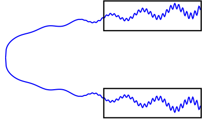
Figure 3. The part of the boundary in the boxes can resemble more and more a fractal as $T\to\infty$.

A well known application of the distortion Theorem 2.3 shows that there exists $K_{1}>0$ such that, for all $t\geq 0$,

(3.7) $$-t+\frac{t\log(|h^{\prime}(1)|)-K_{1}}{\log 1/r}\leq\beta_{h}(r,t)\leq 3t+\frac{t\log\big{(}|h^{\prime}(1)|)+K_{1}}{\log 1/r}\;$$

and a corresponding inequality holds for all $t<0$. Replacing now $h$ by the conformal maps of the family $\mathcal{F}_{\Omega}$, one first has the following observation.

Lemma 3.2.

Let $t\in{\mathbb{R}}$, $R\geq\gamma$ and set $T=R/r$, $r>0$. Then

$$\limsup_{r\to 0}\beta_{\varphi_{R/r}}(r,t)=\limsup_{T\to+\infty}\beta_{\varphi_{T}}(1/T,t)$$

is finite and does not dependent on $R\geq\gamma$.

Proof.

It suffices to treat the case $t>0$ since $t<0$ can be treated the same way and for $t=0$ there is nothing to show. So, let $t>0$ and let $R\geq\gamma$. Finiteness of $\limsup_{r\to 0}\beta_{\varphi_{R/r}}(r,t)$ directly results from (3.4) and (3.7). In order to study the dependence on $R$ of this expression, observe that

$$\beta_{\varphi_{R/r}}(r,t)=\frac{\log\int_{I}|\varphi_{R/r}^{\prime}(r+iy)|^{t}dy}{\log 1/r}=\frac{\log\int_{I}\left(\frac{R/r}{|\varphi(R/r)|}\right)^{t}|\varphi^{\prime}(R+i\frac{R}{r}y)|^{t}dy}{\log 1/r}\,.$$

Since $0<\gamma<1$, it suffices to compare this with the corresponding expression with $R^{\prime}=1$. If $r^{\prime}=r/R$ then

$$\beta_{\varphi_{1/r^{\prime}}}(r^{\prime},t)=\frac{\log\int_{I}|\varphi_{1/r^{\prime}}^{\prime}(r^{\prime}+iy)|^{t}dy}{\log 1/r^{\prime}}=\frac{\log\int_{I}\left(\frac{R/r}{|\varphi(R/r)|}\right)^{t}|\varphi^{\prime}(1+i\frac{R}{r}y)|^{t}dy}{\log 1/r^{\prime}}\,.$$

By Theorem 2.3 there exists $K\geq 1$ such that

$$\frac{1}{KR^{3}}\left|\varphi^{\prime}\left(1+i\tilde{y}\right)\right|\leq\left|\varphi^{\prime}\left(R+i\tilde{y}\right)\right|\leq\left|\varphi^{\prime}\left(1+i\tilde{y}\right)\right|KR$$

for every $\tilde{y}\in{\mathbb{R}}$ and every $R\geq 1$. For $\gamma\leq R<1$ a corresponding estimation holds, we omit this detail and consider $R\geq 1$. Then

$$\frac{-t\log(KR^{3})}{\log 1/r}+\beta_{\varphi_{1/r^{\prime}}}(r^{\prime},t)\frac{\log 1/r^{\prime}}{\log 1/r}\leq\beta_{\varphi_{R/r}}(r,t)\leq\frac{t\log(KR)}{\log 1/r}+\beta_{\varphi_{1/r^{\prime}}}(r^{\prime},t)\frac{\log 1/r^{\prime}}{\log 1/r}$$

from which follows that

$$\limsup_{r\to 0}\beta_{\varphi_{R/r}}(r,t)=\limsup_{r^{\prime}=\frac{r}{R}\to 0}\beta_{\varphi_{1/r^{\prime}}}(r^{\prime},t)\,.$$

∎

We are now ready to introduce the function

(3.8) $$\beta_{\infty}(t)=\limsup_{r\to 0}\beta_{\varphi_{1/r}}(r,t)=\limsup_{T\to+\infty}\beta_{\varphi_{T}}(1/T,t)\quad,\quad t\in{\mathbb{R}}\,.$$

Lemma 3.2 justifies that $t\mapsto\beta_{\infty}(t)$ is a well defined finite function on ${\mathbb{R}}$ and that

(3.9) $$\beta_{\infty}(t)=\sup_{R\geq\gamma}\;\limsup_{r\to 0}\beta_{\varphi_{R/r}}(r,t)\quad,\quad t\in{\mathbb{R}}\,.$$

Up to now we considered a single tract. In the general case we deal with a function $f\in\mathcal{D}$ and so $f^{-1}({\mathbb{D}}^{*})$ is a disjoint union of finitely many tracts $\Omega_{j}$, $j=1,...,N$. Denoting $\beta_{\infty,j}(t)$ the function of (3.8) defined in the tract $\Omega_{j}$, we can associate to $f$ the function

$$\beta_{\infty}=\beta_{\infty,f}:=\max_{j=1,...,N}\beta_{\infty,j}\,.$$

Now we continue dealing with one fixed tract and we skip the index $j$.

Proposition 3.3.

The function $\beta_{\infty}:{\mathbb{R}}\to{\mathbb{R}}$ is convex with

$$\beta_{\infty}(0)=0\ \ \ \text{and }\ \ \beta_{\infty}(2)\leq 1.$$

Proof.

All involved $\beta$–functions are convex by a classical application of Hölder’s inequality (see for example p.176 in [31]). It is trivially obvious that $\beta_{\infty}(0)=0$ while $\beta_{\infty}(2)\leq 1$ results from the well known area estimate. Indeed, let $0<r<1$. For every integer $0\leq k<1/r$ set $y_{k}^{+}:=1+kr$,

$$U_{k}^{+}:=\big{\{}z\in{\mathbb{C}}:r<\Re z<2r\ \ {\rm and}\ \ y_{k}^{+}<\Im z<y_{k+1}^{+}\big{\}}\quad\text{and}\quad U_{k}^{-}:=\big{\{}\overline{z}\;,\,z\in U_{k}^{+}\big{\}}\;.$$

Then,

$$\int_{I}|\varphi_{T}^{\prime}(r+iy)|^{2}dy\asymp\sum_{\begin{subarray}{c}0\leq k<[1/r]\\ \varepsilon\in\{+,-\}\end{subarray}}\frac{1}{r}area(\varphi_{T}(U_{k}^{\varepsilon}))\leq\frac{1}{r}area(\varphi_{T}(Q_{1}\setminus Q_{1/8}))\preceq\frac{1}{r}$$

since $\text{\rm{diam}}\bigl{(}\varphi_{T}(Q_{1}\setminus Q_{1/8})\bigr{)}\preceq 1$. Applying logarithms, dividing by $\log(1/r)$ and letting $r\to 0$ gives that $\beta_{\infty}(2)\leq 1$. ∎

A function related to $\beta_{\infty}$, that will be crucial in the sequel, is the following:

(3.10) $$b_{\infty}(t):=\beta_{\infty}(t)-t+1\quad,\quad t\in{\mathbb{R}}\,.$$

As an immediate consequence of Proposition 3.3 we get the following.

Proposition 3.4.

The function $b_{\infty}:{\mathbb{R}}\to{\mathbb{R}}$ is also convex, thus continuous, with

$$b_{\infty}(0)=1\ \ {\rm and}\ \ b_{\infty}(2)\leq 0.$$

Consequently, the function $b_{\infty}$ has at least one zero in $]0,2]$ and we can introduce a number $\Theta_{f}\in(0,2]$ by

(3.11) $$\Theta_{f}:=\inf\{t>0\;:\;b_{\infty}(t)=0\}=\inf\{t>0\;:\;b_{\infty}(t)\leq 0\}\,.$$

Again, in the case of a function $f$ with finitely many tracts $\Omega_{j}$ we thus have finitely many numbers $\Theta_{f,j}$ and then we set

$$\Theta_{f}:=\max_{j}\Theta_{f,j}.$$

We will consider below various situations and examples illustrating the behavior of $b_{\infty}$ and of $\Theta_{f}$. Notice also that the paper [23] also is based on $\beta_{\infty}$ along with the zero (called also $\Theta$) of $b_{\infty}$.

In order to perform full thermodynamic formalism we need the following crucial property.

Definition 3.5.

A function $f\in\mathcal{D}$ has negative spectrum if

$$b_{\infty}(t)<0\;\text{ for all}\ \ t>\Theta_{f}\,.$$

As we will see in Section 5, this property does hold if the tracts have some nice geometry.

4. Transfer operator

In the sequel $f$ will be either an entire function in $\mathcal{D}$ or a model map in $\mathcal{D}$ and we will work with the Riemannian metric

(4.1) $$|dz|/|z|.$$

This metric is conformally equivalent with the standard Euclidean one, it has singularity at $0$ but is tailor crafted for our analysis of Perron–Frobenius operators. The derivative of a holomorphic function $h$ calculated with respect to the metric of (4.1) at a point $z$ in the domain of $h$ is denoted by $|h^{\prime}(z)|_{1}$ and is given by the formula

(4.2) $$|h^{\prime}(z)|_{1}=|h^{\prime}(z)|\frac{|z|}{|h(z)|}.$$

So, given a real number $t\geq 0$, we define the transfer operator ${\mathcal{L}}_{t}$ by the usual formula:

(4.3) $${\mathcal{L}}_{t}g(w):=\sum_{f(z)=w}|f^{\prime}(z)|^{-t}_{1}g(z)\quad\text{for every}\quad w\in\overline{\Omega}\,$$

where $g$ is any function in $\mathcal{C}_{b}(\overline{\Omega})$, the vector space of all continuous bounded functions defined on $\Omega$. The norm on this space, making it a Banach space, will be the usual sup-norm $\|\cdot\|_{\infty}$. Note that if $w\in\overline{\Omega}$, then $f^{-1}(w)\subset\Omega$, whence $f^{\prime}(z)$ is well defined for all $z\in f^{-1}(w)$ and, in consequence, all terms of the above series are also well defined.

Theorem 4.1.

Let $f$ be a model or an entire function of class $\mathcal{B}$ such that $S(f)\subset{\mathbb{D}}$. Assume that there exists $s>0$ and $w_{0}\in{\mathbb{D}}^{*}$ such that

$${\mathcal{L}}_{t}1\!\!1(w_{0})<\infty\quad\text{for every}\quad t>s\,.$$

Let $\tilde{\gamma}\in(0,1)$. Then

$$\sup_{|w|>e^{\tilde{\gamma}}}{\mathcal{L}}_{t}1\!\!1(w)<\infty\quad\text{for every}\quad t>s\,.$$

In addition, for all $t>s$ and $p>1$ such that $\frac{1}{p}<\frac{t}{s}-1$, there exists a constant $C_{p,t}$ such that

(4.4) $${\mathcal{L}}_{t}1\!\!1(w)\leq\frac{C_{p,t}}{(\log|w|)^{1/p}}\quad\text{for all}\quad w\in{\mathbb{D}}_{e^{\tilde{\gamma}}}^{*}\,.$$

In this result, no dynamical hypothesis nor finiteness of the number of tracts is assumed. If we restrict to functions where $\Omega$ is backward invariant then it tells us that the transfer operators ${\mathcal{L}}_{t}$ are bounded.

Corollary 4.2.

Let $f\in\mathcal{D}$. If there exists $s>0$ and $w_{0}\in\Omega$ such that ${\mathcal{L}}_{t}1\!\!1(w_{0})<\infty$ for all $t>s$, then all ${\mathcal{L}}_{t}$, $t>s$, are bounded operators of $\mathcal{C}_{b}(\overline{\Omega})$, satisfying in addition (4.4).

We will explain in Section 8 that the conclusion of this result combined with our previous work [25] leads to full thermodynamic formalism along with all its usual consequences.

Proof.

Although $f$ may have infinitely many tracts, it suffices to consider the case of a single tract $\Omega$ since the estimates we obtain generalize directly. If $w\in\overline{\mathbb{D}}_{e^{\tilde{\gamma}}}^{*}$ then

(4.5) $${\mathcal{L}}_{t}1\!\!1(w)=\sum_{f(z)=w}|f^{\prime}(z)|^{-t}_{1}\,.$$

The function $f$ restricted to $\Omega$ is of the form $f=e^{\tau}$. Thus

$$|f^{\prime}(z)|_{1}=\frac{|f^{\prime}(z)|}{|f(z)|}|z|=|\tau^{\prime}(z)||z|\,.$$

Since $\varphi=\tau^{-1}$, we have that

$$|f^{\prime}(z)|_{1}=\left|\frac{\varphi(\xi)}{\varphi^{\prime}(\xi)}\right|,$$

where $\xi=\tau(z)$. In the series of (4.5) $z$ runs through the preimages of $w$ under $f$, thus $\xi$ runs through the set $\exp^{-1}(w)$. Let

$$R:=\log|w|=\Re(\xi)$$

for every $\xi\in\exp^{-1}(w)$. We have $R\geq\tilde{\gamma}>0$. We have

(4.6) $${\mathcal{L}}_{t}1\!\!1(w)=\sum_{\xi\in\exp^{-1}(w)}\left|\frac{\varphi^{\prime}(\xi)}{\varphi(\xi)}\right|^{t}=\sum_{\xi\in\exp^{-1}(w)}\left|(\log\varphi)^{\prime}(\xi)\right|^{t}$$

with an arbitrary choice of a holomorphic branch of the logarithm of $\varphi$. Koebe’s Distortion Theorem applied to the conformal map $\log\varphi:\mathcal{H}\to\log\Omega$ gives

(4.7) $${\mathcal{L}}_{t}1\!\!1(w)\asymp\int_{\mathbb{R}}\left|(\log\varphi)^{\prime}(R+iy)\right|^{t}dy$$

On the other hand, $\log\varphi$ is an inverse branch of the logarithmic coordinates of the function $f$ as defined in Section 2 of [15]. Hence, Lemma 1 of [15] applies and yields

$$\left|(\log\varphi)^{\prime}(\xi)\right|\leq\frac{4\pi}{\Re\,\xi}\quad,\quad\xi\in\mathcal{H}\,.$$

In particular, the holomorphic function $u:\mathcal{H}\to{\mathbb{C}}$, defined by

$$u(z):=(\log\varphi)^{\prime}(\frac{\tilde{\gamma}}{2}+z),$$

is bounded and the function $z\mapsto|u(z)|^{t}$ is subharmonic, continuous on $\overline{\mathcal{H}}$ and bounded. We can therefore compare it with its harmonic majorant as it is done in [28, Corollary 10.15]:

(4.8) $$|u(z)|^{t}\leq\frac{1}{\pi}\int_{\mathbb{R}}\frac{x}{(y-s)^{2}+x^{2}}|u(is)|^{t}ds\quad,\quad z=x+iy\in\mathcal{H}\,.$$

Integrating this inequality and using Fubini’s Theorem gives

(4.9) $$\int_{\mathbb{R}}|u(x+iy)|^{t}\,dy\leq\int_{\mathbb{R}}\frac{1}{\pi}\int_{\mathbb{R}}\frac{x}{(y-s)^{2}+x^{2}}dy\,|u(is)|^{t}ds=\int_{\mathbb{R}}|u(is)|^{t}ds<+\infty$$

where the last inequality holds since, by Koebe’s Distortion Theorem and (4.7), the integral on the right hand side is comparable to ${\mathcal{L}}_{t}1\!\!1(w_{0})$, where $w_{0}\in\Omega$ is the point of the assumptions in Theorem 4.1. Therefore, (4.7) along with (4.9) imply that

$${\mathcal{L}}_{t}1\!\!1(w)\preceq{\mathcal{L}}_{t}1\!\!1(w_{0})\quad\text{for every}\quad w\in{\mathbb{D}}_{e^{\tilde{\gamma}}}^{*}.$$

We have thus proved that ${\mathcal{L}}_{t}$ is uniformly bounded on $\overline{\Omega}$.

It remains to show the additional property (4.4). Write $t=\tau+\delta$ where $\tau>s$ and $0<\delta<t-s$. With $x=\log|w|-\tilde{\gamma}/2$, formulas (4.7) and (4.9) imply that

$${\mathcal{L}}_{t}1\!\!1(w)\preceq\frac{1}{\pi}\int_{\mathbb{R}}\int_{\mathbb{R}}\frac{x}{(y-s)^{2}+x^{2}}\,|u(is)|^{\delta}ds\,|u(x+iy)|^{\tau}dy\,.$$

For every $p,q>1$ such that $\frac{1}{p}+\frac{1}{q}=1$ and $p\delta>\Theta_{f}$, Hölder’s inequality yields

$$\int_{\mathbb{R}}\frac{x}{(y-s)^{2}+x^{2}}\,|u(is)|^{\delta}ds\leq\left(\int_{\mathbb{R}}\left(\frac{x}{(y-s)^{2}+x^{2}}\right)^{q}ds\right)^{\frac{1}{q}}\left(\int_{\mathbb{R}}|u(is)|^{\delta p}ds\right)^{\frac{1}{p}}=O(x^{-\frac{1}{p}})\,.$$

Combining the last two displayed formulas, we get

$${\mathcal{L}}_{t}1\!\!1(w)\leq\frac{C_{1}}{x^{1/p}}\int_{\mathbb{R}}|u(x+iy)|^{\tau}dy\leq\frac{C_{2}}{x^{1/p}}\quad\text{for every}\quad w\in{\mathbb{D}}_{e^{\tilde{\gamma}}}^{*}$$

for appropriate constants $C_{1},C_{2}$ depending on $\delta$ and $p$. The proof is now complete since $x=\log|w|-\gamma/2\asymp\log|w|$ for every $w\in{\mathbb{D}}_{e^{\tilde{\gamma}}}^{*}$. ∎

Given Theorem 4.1, the essential question is to decide whether, for a given function $f\in\mathcal{D}$ and parameter $t$, the transfer operator evaluated at $1\!\!1$ is finite or not at some point. This is where our new geometric tools come into play. Aiming to prove Theorem 1.2 we first reformulate ${\mathcal{L}}_{t}$ in terms of the $\beta$–functions.

Proposition 4.3.

If $f\in\mathcal{D}$ and $t\geq 0$, then

$${\mathcal{L}}_{t}1\!\!1(w)\asymp(\log|w|)^{1-t}\left\{\int_{-1}^{1}\left|\varphi_{\log|w|}^{\prime}(1+iy)\right|^{t}dy+\sum_{n\geq 1}2^{n\big{(}1-t+\beta_{\varphi_{2^{n}\log|w|}}(2^{-n},\,t)\big{)}}\right\}$$

for every $w\in\Omega$ with the above series being possibly divergent.

The issue of convergence of the above mentioned series will be the next step.

Proof of Proposition 4.3.

From the proof of Theorem 4.1 we already have the reformulation of the transfer operator that we need in (4.6). Hence

$${\mathcal{L}}_{t}1\!\!1(w)=\sum_{\xi\in\exp^{-1}(w)}\left|\frac{\varphi^{\prime}(\xi)}{\varphi(\xi)}\right|^{t}=\sum_{\xi\in\exp^{-1}(w)|\atop|\Im\xi|<R}\left|\frac{\varphi^{\prime}(\xi)}{\varphi(\xi)}\right|^{t}+\sum_{n\geq 0}\;\sum_{\xi\in\exp^{-1}(w)\atop 2^{n}R\leq|\Im\xi|<2^{n+1}R}\left|\frac{\varphi^{\prime}(\xi)}{\varphi(\xi)}\right|^{t}\,.$$

Applying to each of these sums (2.5) respectively with $T=R$ and $T=2^{n+1}$, $n\geq 0$, we get

(4.10) $${\mathcal{L}}_{t}1\!\!1(w)\asymp\frac{1}{|\varphi(R)|^{t}}\sum_{\xi\in\exp^{-1}(w)|\atop|\Im\xi|<R}\left|\varphi^{\prime}(\xi)\right|^{t}+\sum_{n\geq 0}\frac{1}{|\varphi(2^{n+1}R)|^{t}}\sum_{\xi\in\exp^{-1}(w)|\atop 2^{n}R\leq|\Im\xi|<2^{n+1}R}\left|\varphi^{\prime}(\xi)\right|^{t}\,.$$

Since two consecutive elements of $\exp^{-1}(w)$ are at distance $2\pi$ and since $\Re\xi=R\geq\gamma>0$, Koebe’s Distortion Theorem yields

$${\mathcal{L}}_{t}1\!\!1(w)\asymp\frac{1}{|\varphi(R)|^{t}}\int_{-R}^{R}\left|\varphi^{\prime}(R+iy)\right|^{t}dy+\sum_{n\geq 0}\frac{1}{|\varphi(2^{n+1}R)|^{t}}\int_{I_{n,R}}\left|\varphi^{\prime}(R+iy)\right|^{t}dy$$

where

$$I_{n,R}=[-2^{n+1}R,-2^{n}R]\cup[2^{n}R,2^{n+1}R].$$

Remember that $I=[-2,-1]\cup[1,2]$ and that we have introduced the rescaled functions $\varphi_{R}$ in (3.2). A change of variables gives now

$${\mathcal{L}}_{t}1\!\!1(w)\asymp\;R^{1-t}\int_{-1}^{1}\left|\varphi_{R}^{\prime}(1+iy)\right|^{t}dy+\sum_{n\geq 0}\big{(}2^{n+1}R\big{)}^{1-t}\int_{I}\left|\varphi_{2^{n+1}R}^{\prime}\left(\frac{1}{2^{n+1}}+iy\right)\right|^{t}dy\,.$$

With invoking the definition (3.6) this completes the proof of Proposition 4.3. ∎

Passing to functions having negative spectrum, we can now fully describe the behavior of their transfer operators. As it will be explained in Section 8, this then allows us to prove Theorem 1.2, and its usual consequences, following [25]. We recall that for functions with negative spectrum $\Theta_{f}$ is the unique zero of $b_{\infty}$.

Theorem 4.4.

If $f\in\mathcal{D}$ is a function with negative spectrum, then:

• For every $t>\Theta_{f}$, $\|{\mathcal{L}}_{t}1\!\!1\|_{\infty}<+\infty$ and (4.4) holds.

• For every $t<\Theta_{f}$, the series defining ${\mathcal{L}}_{t}1\!\!1$ is divergent at every point.

Proof.

Let $\gamma$ be the constant from (2.7), let $w_{0}\in{\mathbb{D}}^{*}_{e^{\gamma}}$ be any point and set $R=\log|w_{0}|>\gamma$. Since $f$ has negative spectrum, $b_{\infty}(t)=-2a_{t}<0$ for every $t>\Theta_{f}$. It thus follows right from the definition of $\beta_{\infty}$ in (3.8) that there exist $n_{R,t}>0$ such that

$$\beta_{\varphi_{2^{n}R}}(2^{-n},\,t)-t+1\leq-a_{t}<0\quad\text{for all}\quad n\geq n_{R,t}\,.$$

Applying Proposition 4.3, we get that

$${\mathcal{L}}_{t}1\!\!1(w_{0})<\infty$$

for all $t>\Theta_{f}$. We therefore have checked the hypotheses of Theorem 4.1. It implies that Theorem 4.4 holds for all $t>\Theta_{f}$.

Let now $t<\Theta_{f}$, and $w\in\Omega$ be any point. Set again

$$R:=\log|w|.$$

Then $b_{\infty}(t)=4a_{t}>0$ and thus, by Lemma 3.2,

$$\limsup_{r\to 0}\beta_{\varphi_{R/r}}(r,t)-t+1=4a_{t}>0\;.$$

Fix a sequence $r_{j}\searrow 0$ such that $\beta_{\varphi_{R/r_{j}}}(r_{j},t)-t+1\geq 2a_{t}$ for all $j\geq 1$. Then associate to every $j\geq 0$ an integer $n_{j}$ such that $2^{-n_{j}-1}<r_{j}\leq 2^{-n_{j}}$. Writing down the definition of $\beta_{\varphi_{T}}(r,t)$ and employing (2.5) along with bounded distortion, one gets

$$\lim_{j\to\infty}\;\frac{\beta_{\varphi_{R/r_{j}}}(r_{j},t)}{\beta_{\varphi_{R2^{n_{j}}}}(2^{-n_{j}},t)}=1\,.$$

Thus, $\beta_{\varphi_{R2^{n_{j}}}}(2^{-n_{j}},t)-t+1\geq a_{t}$ for all sufficiently large $j$. This implies that the coefficients in the series in Proposition 4.3 do not converge to zero, whence ${\mathcal{L}}_{t}1\!\!1(w)=\infty$. ∎

5. Functions with negative spectrum and Hölder tracts.

Theorem 1.2 decisively shows that the transfer operators ${\mathcal{L}}_{t}$ of negative spectrum entire functions behave sufficiently well so that a fairly complete account of the corresponding thermodynamic formalism can be derived. In the current section we want to get some idea of which functions in class $\mathcal{D}$ may have negative spectrum. We will start with considering some classical examples such as exponential functions and we will see that the class of balanced functions in [24, 25] behaves like these classical examples (Proposition 5.2); it has the simplest possible $b_{\infty}$ spectrum, namely $b_{\infty}(t)=1-t$. Functions with such spectrum will be called elementary.

Then we will show that a function has negative spectrum as soon as its tracts have some nice geometry. For us it will be Hölder domains. Particular examples of such tracts are quasidisks or tracts having the John or Hölder property used in [23]. We finally show that functions of infinite order can also have negative spectrum, and thus the thermodynamic formalism applies to them too.

5.1. Classical functions and balanced growth

The most classical transcendental family is certainly $\lambda e^{z}$ or, more generally, $\lambda e^{z^{d}}$, $\lambda\in{\mathbb{C}}\setminus\{0\}$, $d\geq 1$. By a straightforward calculation (see also Proposition 5.2), all these functions have a trivial integral means spectrum $\beta_{\infty}\equiv 0$ and thus

(5.1) $$b_{\infty}(t)=1-t\quad,\quad t\in{\mathbb{R}}\,.$$

In particular, they have negative spectrum with $\Theta_{f}=1$ and the tracts of $\lambda e^{z^{d}}$ are not fractal at all. This is also clear when we consider the rescalings. For any tract of such a function, the part of its boundary depicted in the boxes in Figure 3 converges to a straight line segment as $T\to\infty$.

The thermodynamic formalism has been for the first time developed for some transcendental meromorphic functions by Krzysztof Barański in [1]. He did it for for the tangent family. Then this theory has been established for several other families of meromorphic functions. One should mention here quite a large and general class of meromorphic functions considered in [20] where, however, as in [1], there were no singular values of $f^{-1}$ in the Julia which was a compact subset of ${\hat{\mathbb{C}}}$. We also mention [43, 44], where for the first time the thermodynamic formalism was built for a transcendental meromorphic function having such singularity in the Julia set. It was in fact $\infty$ being the asymptotic value of hyperbolic exponential functions. The most general, actually the only general, framework comprising all the classes mentioned above and much more, for which a full fledged thermodynamic formalism has been developed, is up to now the one of [24, 25]. Indeed, these two works cover many classes of entire and meromorphic functions that include such classical functions as exponential family, the ones of the sine and cosine-root family, elliptic functions and all the functions having polynomial Schwarzian derivative. It is based on a condition for the derivative which, for entire functions takes on the following form.

Definition 5.1.

An entire function $f:{\mathbb{C}}\to{\mathbb{C}}$ is said to be of balanced growth if it has finite order, denoted in the sequel by $\rho=\rho(f)$, and if

(5.2) $$|f^{\prime}(z)|\asymp|f(z)|\,|z|^{\rho-1}\quad\text{,}\quad z\in\mathcal{J}_{f}\,.$$

The examples in [24, 25] that satisfy this condition have non-fractal tracts precisely as the classical exponential functions $\lambda e^{z^{d}}$. This is a general fact for balanced functions. They are elementary in the sense that their integral means spectrum $\beta_{\infty}$ is the most trivial possible. In the next result we assume balanced growth on the whole tracts, a condition that is satisfied by all the examples in [24, 25].

Proposition 5.2.

If $f\in\mathcal{D}$ satisfies the balanced condition (5.2) in $\Omega$, then $f$ is elementary in the sense that $\beta_{\infty}\equiv 0$ and thus

$$b_{\infty}(t)=\beta_{\infty}(t)-t+1=1-t\quad,\quad t\in{\mathbb{R}}\,.$$

In particular, $f$ has negative spectrum with $\Theta_{f}=1$.

Proof.

It suffices to consider an entire function or a model function $f\in\mathcal{D}$ with $\Omega$ being one single tract. Then

$$f_{|\Omega}=e^{\tau},$$

where

$$\tau=\varphi^{-1}:\Omega\to\mathcal{H}$$

is a conformal map. Shrinking $\Omega$ if necessary, we may assume that $\tau$ is a continuous map defined on $\overline{\Omega}$. We also may assume that $0\not\in\Omega$ and that a holomorphic branch of $z\mapsto z^{\rho}$ can be well defined on $\Omega$, where $\rho$ comes from (5.2). This allows us to introduce a map

$$h:=\varphi^{\rho}:\mathcal{H}\to\Omega^{\rho}:=\{z^{\rho}\;:\;z\in\Omega\}\,.$$

By assumption, $f$ satisfies (5.2) and $f^{\prime}=f\,\tau^{\prime}$. Therefore,

$$|\varphi^{\prime}(\xi)|=\frac{1}{|\tau^{\prime}(\varphi(\xi))|}\asymp|\varphi(\xi)|^{1-\rho},$$

which implies

(5.3) $$|h^{\prime}(\xi)|=\rho|\varphi(\xi)|^{\rho-1}|\varphi^{\prime}(\xi)|\asymp 1\quad,\quad\xi\in\mathcal{H}\,.$$

As immediate consequence we get that $|h(T)-h(0)|\preceq T$ which implies

(5.4) $$|\varphi(T)|\preceq T^{1/\rho}\quad\text{for}\quad T\geq T_{0}$$

where $T_{0}\geq 1$ is such that $|h(T)|\geq 2|h(0)|$ for $T\geq T_{0}$; it is finite due to (5.3) and Koebe’s $\frac{1}{4}$–Distortion Theorem.

Let $T\geq T_{0}$ and consider $\varphi_{T}$ the rescaled map from (3.2). We have to estimate

$$|\varphi_{T}^{\prime}(\xi)|=\frac{T}{|\varphi(T)|}|\varphi^{\prime}(T\xi)|\asymp\frac{T}{|\varphi(T)|}|\varphi(T\xi)|^{1-\rho}\quad\text{,}\quad\xi\in Q_{1}\setminus Q_{1/8}\,.$$

Assumption (2.5) implies $|\varphi(T\xi)|\asymp|\varphi(T)|$ which then gives

$$|\varphi_{T}^{\prime}(\xi)|\asymp\frac{T}{|\varphi(T)|^{\rho}}\succeq 1\quad\text{,}\quad\xi\in Q_{1}\setminus Q_{1/8}\,,$$

by (5.4). On the other hand, $\frac{T}{|\varphi(T)|^{\rho}}$ is independent of $\xi$. Thus $|\varphi_{T}^{\prime}(\xi)|\asymp|\varphi_{T}^{\prime}(1)|$ and we know from Lemma 3.1 that $|\varphi_{T}^{\prime}(1)|\preceq 1$. Combining all of this gives $|\varphi_{T}^{\prime}|\asymp 1$ on $Q_{1}\setminus Q_{1/8}$ for $T\geq T_{0}$. This readily implies that $\beta_{\infty}\equiv 0$. ∎

5.2. Hölder tracts

Let $f$ be a model as defined in Definition 2.2 or an entire function of class $\mathcal{B}$. Assume that $\Omega$ is a single tract of $f$ and that $\varphi=\tau^{-1}:\mathcal{H}\to\Omega$ the associated conformal map. The rectangles $Q_{T}$ have been introduced in (1.2) and $\Omega_{T}=\varphi(Q_{T})$, $T\geq 1$. A conformal map $g:Q_{1}\to U$ is called $(H,\alpha)$–Hölder if

(5.5) $$|g(z_{1})-g(z_{2})|\leq H|g^{\prime}(1)||z_{1}-z_{2}|^{\alpha}\quad\text{for all}\quad z_{1},z_{2}\in Q_{1}\,.$$

The factor $|g^{\prime}(1)|$ has been introduced in this definition in order to make this Hölder condition scale invariant in the range of $g$.

Definition 5.3.

The tract $\Omega$ is called Hölder, more precisely $(H,\alpha)$–Hölder, if (2.5) holds and if there exists $T_{0}\geq 1$ such that the map $\varphi\circ T:Q_{1}\to\Omega_{T}$ satisfies (5.5) for every $T\geq T_{0}$. We say that $f$ has Hölder tracts if for some $R\geq 1$ the components of $f^{-1}({\mathbb{C}}\setminus\overline{\mathbb{D}}_{R})$ are Hölder tracts.

The main point of this definition is that the tract $\Omega$ is exhausted by a family of uniformly Hölder domains $\Omega_{T}$. We shall prove the following.

Lemma 5.4.

If $f$ is a model or an entire function of class $\mathcal{B}$ and if $\Omega$ is a single Hölder tract of $f$, then

(5.6) $$|\varphi(T)|\asymp\text{\rm{diam}}(\Omega_{T})\asymp|(\varphi\circ T)^{\prime}(1)|\quad,\quad T\geq 1\,,$$

where here and in the sequel, by $\varphi\circ T$ we mean the map given by the formula

$$\varphi\circ T(z)=\phi(Tz).$$

Proof.

The inequality $\text{\rm{diam}}(\Omega_{T})\preceq|(\varphi\circ T)^{\prime}(1)|$ is immediate from (5.5) while the inequality $\text{\rm{diam}}(\Omega_{T})\succeq|(\varphi\circ T)^{\prime}(1)|$ is immediate from Koebe’s $\frac{1}{4}$–Distortion Theorem. Hence

$$|\varphi(T)| \leq|\varphi(T)-\varphi(1)|+|\varphi(1)|\leq H|(\varphi\circ T)^{\prime}(1)|\Big{|}1-\frac{1}{T}\Big{|}^{\alpha}+|\varphi(1)|$$

$$\preceq|\varphi(1)|+\text{\rm{diam}}(\Omega_{T})$$

$$\preceq\text{\rm{diam}}(\Omega_{T}),$$

where the last inequality was written assuming that $T\geq T_{0}$ is large enough, say $T\geq T_{1}\geq T_{0}\geq 1$. We are thus left to show that

(5.7) $$\text{\rm{diam}}(\Omega_{T})\preceq|\varphi(T)|.$$

Indeed, proving this inequality, it follows from (5.5) and the, already proven, right–hand side of (5.6), that

$$\text{\rm{diam}}\bigl{(}\Omega_{8^{-q}T}\bigr{)}\leq\frac{1}{4}\text{\rm{diam}}(\Omega_{T})$$

with some integer $q\geq 1$ and $T\geq T_{1}$ large enough, say $T\geq T_{2}\geq T_{1}$. Therefore, there exist two points $z_{1},z_{2}\in\Omega_{T}\setminus\Omega_{8^{-q}T}$ such that

$$|\varphi(Tz_{2})-\varphi(Tz_{1})|\geq\frac{1}{4}\text{\rm{diam}}(\Omega_{T}).$$

So, applying (2.5) we get that

$$\text{\rm{diam}}(\Omega_{T}) \leq 4|\varphi(Tz_{2})-\varphi(Tz_{1})|\leq 4|\varphi(Tz_{2})|+|\varphi(Tz_{1})|$$

$$\leq 4(M^{q}|\varphi(T)|+M^{q}|\varphi(T)|)$$

$$=8M^{q}|\varphi(T)|,$$

whence formula (5.6) constituting Lemma 5.4 is established. ∎

Remark 5.5.

Invoking Lemma 5.4 we conclude that for a Hölder tract $\Omega$, the functions $\varphi\circ T$ are uniformly Hölder on $Q_{1}$ if and only if the rescaled functions $\varphi_{T}$ satisfy uniformly (5.5) without the factor $|g^{\prime}(1)|$.

We also note that if the components of $f^{-1}({\mathbb{D}}_{R_{0}}^{*})$ are Hölder for some $R_{0}\geq 1$ then the components of $f^{-1}({\mathbb{D}}_{R}^{*})$ are Hölder for all $R\geq R_{0}$. A very important feature of Hölder tracts is expressed by the following.

Proposition 5.6.

All models or functions $f\in\mathcal{B}$ with finitely many Hölder tracts have negative spectrum and

(5.8) $$1\leq\Theta_{f}\leq\text{{\rm HypDim}}(f)\leq 2\;.$$

In addition, if the corresponding Hölder exponent $\alpha\in(1/2,1]$, then $\Theta_{f}<2$.

Proof.

A classical argument (see [31] or the proof of Proposition 3.3 in [23]) applies word for word showing that

(5.9) $$\beta_{\infty}(t+s)\leq(1-\alpha)s+\beta_{\infty}(t),$$

where, we recall, $\alpha$ is a Hölder exponent of the tract $\Omega$. Therefore,

(5.10) $$b_{\infty}(t+s)\leq b_{\infty}(t)-\alpha s.$$

Thus $b_{\infty}(t)<0$ for all $t>\Theta_{f}$ which shows that $f$ has negative spectrum.

As explained before, the paper [23] also employs the same $b_{\infty}$–function along with the zero $\Theta_{f}$ and Theorem 1.1 of [23] shows that (5.8) holds for Hölder tracts.

The second to last assertion of Proposition 3.4 is that $b_{\infty}(0)=1$. So, with $t=0$ and $s=2$, it follows from (5.10) that $b_{\infty}(2)\leq 1-2\alpha<0$ whenever $\alpha>1/2$, and thus that $\Theta_{f}<2$. The proof is complete. ∎

All the elementary functions enjoy the property that $\Theta_{f}=1$ but in general Hölder tracts are fractal in the sense that

$$\Theta_{f}>1\,.$$

Models with fractal tracts have been considered in [23]. A particular family of entire functions having fractal tracts is studied in detail in the forthcoming Section 7.

5.3. Functions of infinite order

Let us finally consider one other family of examples having totally different behavior than the preceding ones. They have tracts that are not Hölder, they are of infinite order and also the family of rescalings $\mathcal{F}_{\Omega}$ has only constant limit functions. Nevertheless, we will see that they have negative spectrum and thus they are first examples of infinite order for which the thermodynamic formalism is developed.

Consider functions $f\in\mathcal{D}$, no matter whether entire or model, having the following properties:

• $f$ has negative spectrum.

• $f$ has a Hölder tract $\Omega_{f}\subset\{\Re z\geq 3\}\subset\mathcal{H}$.

We will associate to such a function a model function $F$ defined on $\Omega_{F}=\log(\Omega_{f})$, $\log$ meaning any, or even finitely many, arbitrary branches of the logarithm. The definition of $F$ is this.

$$F:=f\circ\exp:\Omega_{F}\to{\mathbb{C}}\,.$$

To such a function Theorem 1.2 applies since we have the following.

Proposition 5.7.

The infinite order function $F=f\circ\exp:\Omega_{F}\to{\mathbb{C}}$ belongs to $\mathcal{D}$ and has negative spectrum with $\Theta_{F}=\Theta_{f}$.

Proof.

The disjoint type property follows since $F^{-1}({\mathbb{D}}^{*})=\Omega_{F}\subset{\mathbb{D}}^{*}$. Let $\varphi=\tau^{-1}:\mathcal{H}\to\Omega_{f}$ be conformal such that $f=e^{\tau}$ on $\Omega_{f}$. Then

$$F=\exp\circ(\tau\circ\exp).$$

It suffices to consider the case where $\Omega_{F}$ is a single tract so that $\tau\circ\exp:\Omega_{F}\to\mathcal{H}$ is a conformal map with inverse $\Phi=\log\circ\,\varphi$. Since $f\in\mathcal{D}$ it satisfies (2.5) and since $\Omega_{f}\subset\{\Re z\geq 3\}$ we have

$$\frac{|\Phi(\xi_{1})|}{|\Phi(\xi_{2})|}=\frac{\log|\varphi(\xi_{1})|}{\log|\varphi(\xi_{2})|}\leq 1+\frac{\log M}{\log|\varphi(\xi_{2})|}\leq 1+\frac{\log M}{\log 3}\quad\text{for all}\quad\xi_{1},\xi_{2}\in Q_{T}\setminus Q_{T/8}\,.$$

Thus $\Phi$ satisfies (2.5), completing the argument that $F$ is in $\mathcal{D}$.

It remains to estimate $\beta_{\infty,F}$. For $T\geq 1$, $\Phi_{T}=\frac{1}{|\Phi(T)|}\log\circ\varphi\circ T$ hence

$$\Phi_{T}^{\prime}(\xi)=\frac{T}{|\Phi(T)|}\frac{\varphi^{\prime}(T\xi)}{\varphi(T\xi)}=\frac{1}{|\log\varphi(T)|}\frac{|\varphi(T)|}{\varphi(T\xi)}\,\varphi_{T}^{\prime}(\xi)$$

thus

$$|\Phi_{T}^{\prime}(\xi)|\asymp\frac{1}{\log|\varphi(T)|}|\varphi_{T}^{\prime}(\xi)|\quad\text{for every}\quad\xi\in Q_{1}\setminus Q_{1/8}\,.$$

The factor $|\varphi(T)|$ can be estimated as follows. Still since $\Omega_{f}\subset\{\Re z\geq 3\}$ we have $|\varphi(T)|\geq 3$. On the other hand we have from (2.10)

$$|\varphi(T)|\preceq|\varphi(T)-\varphi(1)|\leq T^{2}|\varphi^{\prime}(1)|\,.$$

It follows that there exists a constant $C\geq 0$ such that

$$\frac{e^{-C}}{\log T}\int_{I}|\varphi_{T}^{\prime}(r+iy)|^{t}dy\leq\int_{I}|\Phi_{T}^{\prime}(r+iy)|^{t}dy\leq e^{C}\int_{I}|\varphi_{T}^{\prime}(r+iy)|^{t}dy$$

for every $r\in(0,1)$ and $T\geq 1$. Setting now $T=1/r$, taking logarithm of the preceding inequality and dividing it then by $\log 1/r$ shows that

$$\frac{-C-\log\log 1/r}{\log 1/r}+\beta_{\varphi_{1/r}}(r,t)\leq\beta_{\Phi_{1/r}}(r,t)\leq\beta_{\varphi_{1/r}}(r,t).$$

Since the first term on the left hand side of this inequality goes to zero as $r\to 0$ we get $\beta_{\infty,F}(t)=\beta_{\infty,f}(t)$ from which the Proposition follows. ∎

6. Quasiconformal invariance of Hölder tracts

Quasiconformal maps have good Hölder continuity properties and thus preserve Hölder tracts. Let us make this precise.

Lemma 6.1.

Let $g,f\in\mathcal{B}$ have finitely many tracts and assume that there is $R\geq 1$ such that all the connected components of $g^{-1}({\mathbb{D}}_{R}^{*})$ are Hölder. If $\Phi:{\mathbb{C}}\to{\mathbb{C}}$ is a quasiconformal homeomorphism such that

$$f^{-1}({\mathbb{D}}_{R}^{*})=\Phi\left(g^{-1}({\mathbb{D}}_{R}^{*})\right)\quad\text{and}\quad f\circ\Phi=g\quad\text{on}\quad g^{-1}({\mathbb{D}}_{R}^{*})$$

then all the connected components of $f^{-1}({\mathbb{D}}_{R}^{*})$ are Hölder.

Proof.

It suffices to consider the case where the functions have just one tract $\Omega_{g}=g^{-1}(D_{R}^{*})$ and $\Omega_{f}=\Phi(\Omega_{g})$. We may also assume without loss of generality that $R=1$. Then there are conformal maps $\varphi_{g}:\mathcal{H}\to\Omega_{g}$ and $\varphi_{f}:\mathcal{H}\to\Omega_{f}$ such that, with appropriate holomorphic branches of logarithms, the holomorphic maps $\log g:\Omega_{g}\to\mathcal{H}$ and $\log f:\Omega_{f}\to\mathcal{H}$ are the respective inverses of $\varphi_{g}$ and $\varphi_{f}$, and, in addition,

$$\varphi_{f}=\Phi\circ\varphi_{g}\,.$$

By our hypotheses, $\varphi_{g}$ satisfies the conditions of Definition 5.3 and we have to show that $\varphi_{f}$ does it too. The condition (2.5) is satisfied by $\varphi_{g}$ and $|\varphi_{g}(T)|\to\infty$ as $T\to\infty$. Thus

(6.1) $$|\varphi_{g}(\xi_{1})-\varphi_{g}(0)|\asymp|\varphi_{g}(\xi_{1})|\leq M|\varphi_{g}(\xi_{2})|\asymp|\varphi_{g}(\xi_{2})-\varphi_{g}(0)|$$

for all $\xi_{1},\xi_{2}\in Q_{T}\setminus Q_{T/8}$, $T\geq 8$. Since the map $\Phi$ is quasiconformal, it is quasisymmetric. This means that there exists a homeomorphism $\eta:[0,\infty)\to[0,\infty)$ such that $|a-b|\leq t|a-c|$ yields

$$|\Phi(a)-\Phi(b)|\leq\eta(t)|\Phi(a)-\Phi(c)|.$$

Along with (6.1), this gives that

$$|\varphi_{f}(\xi_{1})| =|\Phi(\varphi_{g}(\xi_{1}))|\asymp|\Phi(\varphi_{g}(\xi_{1}))-\Phi(\varphi_{g}(0))|$$

$$\leq\eta(M^{\prime})|\Phi(\varphi_{g}(\xi_{2}))-\Phi(\varphi_{g}(0))|$$

$$\asymp|\Phi(\varphi_{g}(\xi_{2}))|$$

$$=|\varphi_{f}(\xi_{2})|$$

for all $\xi_{1},\xi_{2}\in Q_{T}\setminus Q_{T/8}$, $T\geq 8$, where $M^{\prime}$ is a constant witnessing the comparability of the very left and the very right sides of (6.1). In other words, $\varphi_{f}$ satisfies (2.5).

We know that for some $T_{0}\geq 1$ the family of rescalings $\varphi_{g,T}$, $T\geq T_{0}$, of $\varphi_{g}$ is uniformly Hölder and it remains to show that

$$\varphi_{f,T}=\frac{1}{|\Phi(\varphi_{g}(T))|}\,\Phi\circ|\varphi_{g}(T)|\circ\varphi_{g,T}\quad,\quad T\geq T_{0}\,,$$

has the same property. All the mappings

$$\hat{g}_{T}:=\frac{1}{|\Phi(\varphi_{g}(T))|}\,\Phi\circ|\varphi_{g}(T)|$$

are $K$–quasiconformal, where $K$ is the quasiconformal constant of $\Phi$ and they are normalized by $\hat{g}_{T}(\infty)=\infty$. We shall prove the following.

Claim: There exists a constant $\kappa\in(0,1]$ such that

$$|\hat{g}_{T}(0)|\leq\kappa\leq 2\kappa\leq|\hat{g}_{T}(1)|\leq 1/\kappa\quad\text{ for all $T\geq T_{0}$.}$$

Proof.

We have

$$|\Phi(|\varphi_{g}(T)|)|\asymp|\Phi(|\varphi_{g}(T)|)-\Phi(0)||\ \ \ {\rm and}\ \ \ |\Phi(\varphi_{g}(T))|\asymp|\Phi(\varphi_{g}(T))-\Phi(0)||,$$

and obviously $|\varphi_{g}(T)-0|=\big{|}|\varphi_{g}(T)|-0\big{|}.$ Therefore, invoking again quasisymmetricity of $\Phi$, witnessed by the homeomorphism $\eta:[0,\infty)\to[0,\infty)$, we consecutively get

$$\frac{1}{\eta(1)}\leq\frac{|\Phi(|\varphi_{g}(T)|)-\Phi(0)||}{|\Phi(\varphi_{g}(T))-\Phi(0)||}\leq\eta(1)$$

and

$$\frac{|\Phi(|\varphi_{g}(T)|)|}{|\Phi(\varphi_{g}(T))|}\asymp 1.$$

This means that $|\hat{g}_{T}(1)|\asymp 1.$ The proof of the Claim is complete. ∎

In conclusion,

$$\mathcal{G}:=\{g_{T}:T\geq T_{0}\}$$

is a uniformly quasiconformal and normalized family. By Remark 5.5 there exists $R>1$ such that

$$\varphi_{g,T}(Q_{1})\subset\overline{\mathbb{D}}_{R}$$

for all $T\geq T_{0}$. These two facts imply (see Theorem 4.3 in [21]) that the family $\mathcal{G}$ restricted to $\overline{\mathbb{D}}_{R}$ is uniformly Hölder. Therefore, $\varphi_{f,T}$ is uniformly Hölder as a composition of two Hölder functions whose Hölder exponents and constants do not depend on $T\geq T_{0}$. ∎

We provide two important applications of the quasiconformal invariance of Hölder tracts. The first one we present right now and it concerns quasiconformal approximation. The second application will be in Section 10 on analytic families of functions in the Speiser class $\mathcal{S}$.

6.1. Quasiconformal approximation

As already mentioned, Bishop [9, 10] considered quasiconformal approximations of most general models where $\Omega$ can be an arbitrary union of simply connected unbounded domains. Keeping our definition of a model, the following result is a simplified version of Theorem 1.1 in [9].

Theorem 6.2 ([9]).

Let $(\tau,\Omega)$ be a tract model and $f=e^{\tau}$ the corresponding function. Fix $R>0$. Then there exist an entire function $F\in\mathcal{B}$ and a quasiconformal map $\psi:{\mathbb{C}}\to{\mathbb{C}}$ with $\psi$ conformal outside of $\{z\in{\mathbb{C}}:R<\Re\tau(z)<2R\}$ such that

$$e^{\tau}=F\circ\psi$$

on $\Omega(2R)=\{z\in{\mathbb{C}}:\Re\tau(z)>2R\}$. Moreover, the components of $\{|F|>e^{R}\}$ are in a $1$-to-$1$ correspondence with the components of $\Omega$ via $\psi$.

If the initial model is of disjoint type one can adjust $R>0$ such that

(6.2) $$\mathcal{J}_{f}\subset\Omega(3R)=\{z\in{\mathbb{C}}:\Re\tau(z)>3R\}\,.$$

Then we can assume that $F$ also is of disjoint type since otherwise it suffices to compose $\psi$ with an affine map. So, we can consider for the map $F$ the set of tracts $\Omega_{F}=\psi(\Omega(2R))$ and suppose that $\mathcal{J}_{F}\subset\psi(\Omega(3R))$.

Proposition 6.3.

Suppose $f\in\mathcal{D}$ is a model having only Hölder tracts and suppose that $F$ is a disjoint type entire function given by Bishop’s Theorem 6.2 with $R>0$ small enough such that (6.2) holds. Then, $F\in\mathcal{D}$, the tracts $\Omega_{F}$ of $F$ are Hölder and consequently $F$ has negative spectrum.

Proof.

Follows directly from Lemma 6.1. ∎

7. Poincaré functions

In this section, we consider a, quite particular, family of entire functions. They are obtained by linearization of a polynomial at a repelling fixed point and are often called linearizers or Poincaré functions (see [12, 29, 14]). We first consider general linearizers and then show that these functions have negative spectrum if and only if the corresponding polynomial is topologically Collet-Eckmann (TCE).

7.1. Linearizers: the general case.

Let $p:{\hat{\mathbb{C}}}\to{\hat{\mathbb{C}}}$ be a polynomial having a repelling fixed point $z_{0}$ with multiplier $\lambda=p^{\prime}(z_{0})$. By the Koenigs-Poincaré linearization theorem there exists an entire function $f:{\mathbb{C}}\to{\mathbb{C}}$ such that

(7.1) $$f(0)=z_{0}\quad\text{and}\quad f(\lambda z)=p\circ f(z)\quad,\quad z\in{\mathbb{C}}.$$

We then call $f$ linearizer of $p$ or, more precisely, linearizer of $p$ at the fixed point $z_{0}$.

Remark 7.1.

One could consider here a much more general family. Instead of linearizing the dynamics at a repelling fixed point one can consider limits of rescalings at conical limit points. For example, if $p$ is a hyperbolic polynomial with connected Julia set then there exist entire linearizers at any point of the Julia set $\mathcal{J}_{p}$ (see [5, Theorem 2.10]).

We only will consider the case where the Julia set of $p$ is connected. Then $\text{{\rm P}}(p)$, the post–singular set of $p$, is a subset of the filled Julia set and thus a subset of the complement of $A_{p}(\infty)$, the attracting bassin of infinity. Since the set of singular values of $f$ is equal to the post–singular set of $p$ (see Proposition 3.2 in [29]) it follows that $f$ belongs to class $\mathcal{B}$. Up to normalization we can assume that $\mathcal{J}_{p}\subset{\mathbb{D}}$ or, equivalently, that ${\mathbb{D}}^{*}\subset A_{p}(\infty)$. Then $S(f)\subset{\mathbb{D}}$ and we can consider the set of tracts $\Omega=f^{-1}({\mathbb{D}}^{*})$. Conjugating eventually $p$ by an affine map, we also may assume without loss of generality that

$$z_{0}\neq 0\; \;0\not\in A_{p}(\infty)$$ and that .

Linearizers of polynomials are entire functions of finite order [45] and the Denjoy–Carleman–Ahlfors Theorem asserts that finite order functions have only finitely many tracts $\Omega_{j}\subset\Omega$, $j=1,...,N$. Let $\hat{\Omega}_{j}$ be the connected component of $f^{-1}(A_{p}(\infty))$ that contains $\Omega_{j}$. It follows from $p$–invariance of $A_{p}(\infty)$ along with (7.1) that multiplication by $\lambda$ permutes the finitely many components $\hat{\Omega}_{j}$ (see also Proposition 2.1 of [18] for a different approach to this fact). Replacing $p$, hence $\lambda$, by an iterate we may assume that

$$\lambda\hat{\Omega}_{j}=\hat{\Omega}_{j}\; \;j=1,...,N$$ for every .

It thus suffices to consider in the following a single tract. We will call it $\Omega$, thus from now on $\Omega$ will be a connected component of $f^{-1}({\mathbb{D}}^{*})$ and $\hat{\Omega}$ will be the component of $f^{-1}(A_{p}(\infty))$ that contains $\Omega$. Recalling that $0\notin A_{p}(\infty)$, we see that the function $f$ restricted to $\hat{\Omega}$ is again of the form $f=e^{\varphi^{-1}},$ where $\varphi:\hat{\mathcal{H}}\to\hat{\Omega}$ is a conformal homeomorphism and $\Omega=\varphi(\mathcal{H})$.

Since $\mathcal{J}_{p}$ is connected, there exists a conformal map $h:{\mathbb{D}}^{*}\to A_{p}(\infty)$ such that

(7.2) $$h(1)=z_{0}\quad\text{and}\quad p\circ h(z)=h(z^{d})\quad,\quad z\in{\mathbb{D}}^{*},$$

where $d\geq 2$ is the degree of the polynomial $p$. Notice that here $h(1)$ must be properly defined since the Julia set $\mathcal{J}_{p}$ may fail to be locally connected and then $h$ has no continuous extension to the boundary. However, since $z_{0}$ is repelling there exists an external ray $\mathcal{R}_{t}=h(\{re^{it}\,;\;r>1\})$ who lands at $z_{0}$. Such a ray can be obtained by constructing first a $\lambda$–invariant curve in the tract $\hat{\Omega}$ which then can be projected down by $f$ (see Section 2.3 of [18]). In our situation we may assume that $t=0$ and then the normalization in (7.2) is defined with the radial limit $\lim_{r\searrow 1}h(r)=z_{0}$.

The map $h$ can be lifted, via the exponential map, to a conformal homeomorphism

$$H:\mathcal{H}\to\hat{\mathcal{H}}:=\exp^{-1}(A_{p}(\infty))$$

that commutes with translation by $2\pi i$, i.e. $H(z+2\pi i)=H(z)+2\pi i$ for all $z\in\mathcal{H}$, and such that

(7.3) $$\varphi\circ H(0)=0\quad\text{and}\quad\exp\circ H=h\circ\exp\quad on\quad\mathcal{H}\,.$$

Lemma 7.2.

The inverse conformal map $H^{-1}:\hat{\mathcal{H}}\to\mathcal{H}$ is bi–Lipschitz on the half–space $\{\Re z>s\}$, whenever $s\in{\mathbb{R}}$ is such that $\{z\in{\mathbb{C}}:\Re z\geq s\}\subset\hat{\mathcal{H}}$.

Proof.

Indeed, with $\tilde{h}(z):=1/h(1/z)$, $z\in{\mathbb{D}}$,

$$H^{\prime}(z)=\frac{e^{-z}}{\tilde{h}(e^{-z})}\tilde{h}^{\prime}(e^{-z})\longrightarrow 1\quad\text{when}\quad\Re z\to+\infty\,.$$

This and the $2\pi i$–periodicity of $H$ imply the announced bi–Lipschitz property. ∎

Since $\overline{\mathbb{D}}^{*}\subset A_{p}(\infty)$, there exists $t<0$ such that

(7.4) $$\overline{\mathcal{H}}\subset\{\Re z>t\}\subset\hat{\mathcal{H}}\,.$$

Consequently, $H^{-1}$ is uniformly bi–Lipschitz, say with constant $L\geq 1$, on all the rectangles $Q_{T}$, $T\geq 1$.

Recall that $\lambda$ is the multiplier of $p$ at the repelling fixed point $z_{0}$. Since $f$ conjugates multiplication by $\lambda$ and the polynomial $p$, since $h$ satisfies (7.2) and the right hand sided part of (7.3), and since the exponential map lifts $z\mapsto z^{d}$ to multiplication by $d$, we get

$$f\big{(}\varphi\circ H(dz)\big{)}=h\big{(}e^{dz}\big{)}=p\big{(}h(e^{z})\big{)}=p\big{(}f(\varphi\circ H)(z)\big{)}=f\big{(}\lambda(\varphi\circ H)(z)\big{)}\,\text{ for all $z\in\mathcal{H}$.}$$

Along with the left hand side of (7.3) this implies that

(7.5) $$\big{(}\varphi\circ H\big{)}(dz)=\lambda\,\big{(}\varphi\circ H\big{)}(z)\quad,\quad z\in\mathcal{H}\,.$$

Indeed, both $\varphi\circ H\circ d$ and $\lambda(\varphi\circ H)$ are conformal mappings from $\mathcal{H}$ onto $\hat{\Omega}$ and (7.5) holds near the origin. In conclusion, we have the commutative diagram of Figure 4.

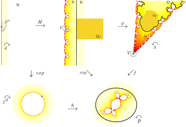
Figure 4. Linearizing Douady’s Rabbit

As a final preliminary remark we recall that a linearizer is essentially unique. Indeed, if $f$ has the property (7.1), then every other solution of (7.1) is of the form $f_{\kappa}=f\circ\kappa$ for some $\kappa\in{\mathbb{C}}^{*}$.

Theorem 7.3.

If $p$ is a polynomial with connected Julia set, if $f_{\kappa}=f\circ\kappa$ is a linearizer of $p$ at a repelling fixed point $z_{0}$ and if $\kappa$ is sufficiently small, then, up to normalization, $\mathcal{J}_{f_{\kappa}}\subset{\mathbb{D}}^{*}\subset A_{p}(\infty)$ and the following holds:

1. $f_{\kappa}\in\mathcal{D}$.

2. $\Theta_{f_{\kappa}}=\text{{\rm HypDim}}(p)$, the hyperbolic dimension of $p$.

3. The tracts of $f_{\kappa}$ are fractal in the sense that

   $$\Theta_{f_{\kappa}}>1$$

   if and only if $p$ is not an exceptional polynomial.

Recall that a polynomial is called exceptional if it is either of the form $z\mapsto z^{d}$, $d\geq 2$, or it is a Tchebychev polynomial. Such polynomials are special in the sense that Zdunik [46] has shown that they are the only polynomials for which the harmonic measure, viewed from infinity, is not singular with respect to the natural Hausdorff measure of the Julia set.

Theorem 7.3 will be shown in two steps. It will be a consequence of the next Lemma along with Proposition 7.5.

Lemma 7.4.

If $p$ is a polynomial with connected Julia set and if $f_{\kappa}=f\circ\kappa$ is a linearizer of $p$ at a repelling fixed point $z_{0}$ then $f_{\kappa}\in\mathcal{D}$ provided $\kappa$ is sufficiently small and, up to normalization, $\mathcal{J}_{f_{\kappa}}\subset{\mathbb{D}}^{*}\subset A_{p}(\infty)$.

Proof.

By the above discussion, we already know the following facts: the linearizers $f_{\kappa}$ are of finite order and thus have only finitely many tracts, they belong to class $\mathcal{B}$ and, normalizing $p$ if necessary, $\mathcal{J}_{f_{\kappa}}\subset{\mathbb{D}}^{*}\subset A_{p}(\infty)$. Furthermore, for small values of $\kappa$ the function $f_{\kappa}$ is of disjoint type and, in order to verify that it belongs to class $\mathcal{D}$, it remains to verify (2.5). Notice that this condition is equivalent to the following: there exists $C>1$ and $M<\infty$ such that

(7.6) $$\text{$\forall\xi,\xi^{\prime}\in\mathcal{H}\;$ with }\;\frac{1}{C}<\frac{|\xi|}{|\xi^{\prime}|}<C\quad\text{have}\quad|\varphi(\xi)|\leq M|\varphi(\xi^{\prime})|\,.$$

Moreover, if (7.6) holds for some $C>1$ then it does hold for all $C>1$ (and for some $M=M(C)<\infty$). Since here $\varphi=(\varphi\circ H)\circ H^{-1}_{|\mathcal{H}}$ it suffices to verify separately (7.6) for $H^{-1}_{|\mathcal{H}}$ and for $\varphi\circ\text{{\rm H}}$. Then clearly the composition $(\varphi\circ H)\circ H^{-1}_{|\mathcal{H}}$ also satisfies (7.6) (with different constants).

For $H^{-1}_{|\mathcal{H}}$ this directly follows from the bi-Lipschitz property in Lemma 7.2: let $C>1$ and $\xi,\xi^{\prime}\in\mathcal{H}$ with $\frac{1}{C}<\frac{|\xi|}{|\xi^{\prime}|}<C$. Then, for all $\xi\in\mathcal{H}$,

(7.7) $$\frac{1}{L}|\xi|-|H^{-1}(0)|\leq|H^{-1}(\xi)|=|H^{-1}(\xi)-H^{-1}(0)+H^{-1}(0)|\leq L|\xi|+|H^{-1}(0)|$$

hence, if $|\xi|,|\xi^{\prime}|\geq 2L|H^{-1}(0)|$,

$$\frac{1}{C}\frac{\frac{1}{2L}}{L+\frac{1}{2L}}\leq\frac{|H^{-1}(\xi)|}{|H^{-1}(\xi^{\prime})|}\leq\frac{\left(L+\frac{1}{2L}\right)|\xi|}{\left(\frac{1}{L}-\frac{1}{2L}\right)|\xi^{\prime}|}\leq\frac{\left(L+\frac{1}{2L}\right)}{\left(\frac{1}{L}-\frac{1}{2L}\right)}C$$

which implies the required inequality with $M=\frac{L+1/(2L)}{1/L-1/(2L)}C$ in this case. If one of the points $\xi,\xi^{\prime}$ has modulus smaller than $2L|H^{-1}(0)|$ then both have modulus smaller than $s=2L|H^{-1}(0)|C$ and then the required inequality follows since for the compact subset $K=\overline{{\mathbb{D}}_{s}\cap\mathcal{H}}$ of $\hat{\mathcal{H}}$ one clearly has $\inf_{K}|H^{-1}|>0$ and $\sup_{K}|H^{-1}|<\infty$.

It remains to proof (7.6) for the map $\varphi\circ H$. This map conjugates multiplication by $d$ and multiplication by $\lambda$ (see (7.5)). The set $A=\{\xi\in\mathcal{H}\;,\;1<|\xi|\leq d\}$ is a fundamental set for the multiplication by $d$ in $\mathcal{H}$, $A^{\prime}=\varphi\circ H(A)\subset\hat{\Omega}\subset{\mathbb{C}}^{*}$ and $A^{\prime}/<\lambda>$ is an annulus of the torus ${\mathbb{C}}^{*}/<\lambda>$ (whose precise description is given in [18]). Consequently, $\overline{A^{\prime}}$ is a compact subset of ${\mathbb{C}}^{*}$ as well as the set $\lambda^{k}\overline{A^{\prime}}=\overline{\varphi\circ H(d^{k}A)}$, $k\in{\mathbb{Z}}$.

Let $C>1$ and let $\mathcal{A}=\Big{\{}\frac{1}{C}\leq|\xi|\leq Cd\;,\;\xi\in\mathcal{H}\Big{\}}$. This set can be covered by finitely many sets $d^{k}A$ and thus $\overline{\varphi\circ H(\mathcal{A})}$ is also compact in ${\mathbb{C}}^{*}$. Therefore, there exists $0<\underline{m}\leq\overline{m}<\infty$ such that

(7.8) $$\underline{m}\leq|\varphi\circ H(\xi)|\leq\overline{m}\quad\text{for all}\quad\xi\in\mathcal{A}=\Big{\{}\frac{1}{C}\leq|\xi|\leq Cd\;,\;\xi\in\mathcal{H}\Big{\}}.$$

Now, let $\xi,\xi^{\prime}$ be like in (7.6) and choose $k\in{\mathbb{Z}}$ such that $1<|d^{k}\xi|\leq d$. Then $d^{k}\xi,d^{k}\xi^{\prime}\in\mathcal{A}$ and thus (7.5) and (7.8) imply that

$$\frac{|\varphi\circ H(\xi)|}{|\varphi\circ H(\xi^{\prime})|}=\frac{|\varphi\circ H(d^{k}\xi)|}{|\varphi\circ H(d^{k}\xi^{\prime})|}\leq\frac{\overline{m}}{\underline{m}}.$$

This completes the proof since it shows that $\varphi\circ H$ also satisfies (7.6). ∎

The second and final step of the proof of Theorem 7.3 is the following.

Proposition 7.5.

Let $p$ be a polynomial with connected Julia set and let $f$ be a linearizer of $p$ that satisfies the conclusions of Lemma 7.4. Then,

1. $\Theta_{f}=\text{{\rm HypDim}}(p)$, the hyperbolic dimension of $p$.

2. The tracts of $f$ are fractal in the sense that

   $$\Theta_{f}>1$$

   if and only if $p$ is not an exceptional polynomial.

A key point in the proof of this result is that we will be able to relate the $\beta_{\infty}$ function of the rescalings to the classical integral means spectrum

$$\beta_{h}(t)=\limsup_{r\to 1^{+}}\frac{\log\int_{|z|=1}|h^{\prime}(rz)|^{t}|dz|}{-\log(r-1)}$$

of the Riemann map $h:\{|z|>1\}\to A_{p}(\infty)$ of (7.2). For this function there is a formula holding for all polynomials with connected Julia sets (see [8], see also [36] for the expanding case):

(7.9) $$\beta_{h}(t)-t+1=\frac{\text{{\rm P}}(t)}{\log d}$$

where $d:=\deg(p)$ and $\text{{\rm P}}(t)$ is the topological pressure of the potential $-t\log|p^{\prime}|$ with respect to the polynomial $p$. In fact $\text{{\rm P}}(t)$ is the tree pressure in the general non-expanding case, see [32, 35]. Since this formula does not directly hold here, we provide its suitable variant along with all the details in the Appendix A.

Proof.

In order to relate these spectra we have to study in detail the rescaled functions $\varphi_{T}$ and thus $\varphi$. We start with a preliminary observation. If $\exp_{*}^{-1}$ is the holomorphic inverse branch of the exponential map, defined near $z_{0}$, such that $\exp_{*}^{-1}(z_{0})=\tau(0)$, then $\exp_{*}^{-1}\circ f$ extends $\tau=\varphi^{-1}$ to some bounded open neighborhood, call it $V$, of the origin. Since $f^{\prime}(0)\neq 0$, the neighborhood $V$ can be chosen such that $\tau:V\to V^{\prime}=\tau(V)$ is bi–Lipschitz. Then

(7.10) $$|\varphi^{\prime}|\asymp 1\quad\text{ in }\quad V^{\prime}.$$

Again (7.5) shows that $\varphi=(\varphi\circ H)\circ H^{-1}_{|\mathcal{H}}=\lambda^{N}(\varphi\circ H)\circ d^{-N}\circ H^{-1}$ and thus

$$\varphi\circ T_{|Q_{1}}=\lambda^{N}(\varphi\circ H)\circ(d^{-N}\circ H^{-1}\circ T)_{|Q_{1}}:Q_{1}\to\Omega_{T}$$

for every $N\in{\mathbb{Z}}$. Given $T\geq 1$, we fix this integer as follows. Let $A$ be again the fundamental set for the multiplication by $d$ in $\mathcal{H}$ of the proof of Lemma 7.4 and $A^{\prime}=\varphi\circ H(A)$. Let then $N_{0}=N_{0}(T)\in{\mathbb{Z}}$ be the unique integer such that

(7.11) $$\lambda^{-N_{0}}\varphi(T)\in A^{\prime}\quad\text{or, equivalently, such that}\quad d^{-N_{0}}H^{-1}(T)\in A.$$

Since $H^{-1}_{|\mathcal{H}}$ is bi-Lipschitz we have, by the same argument than in (7.7), that

(7.12) $$T\asymp d^{N_{0}}\quad\text{uniformly in $T\geq 1$}$$

and thus we see that the map $d^{-N_{0}}\circ H^{-1}\circ T$ is uniformly bi-Lipschitz on $Q_{1}$. On the other hand, (7.8) implies that

(7.13) $$\underline{m}\leq|\lambda|^{-N_{0}}|\varphi(T)|\leq\overline{m}$$

thus, using (2.5),

$$\frac{\underline{m}}{M}\leq|\lambda|^{-N_{0}}|\varphi(\xi)|\leq M\overline{m}\quad\text{for all}\quad\xi\in Q_{T}\setminus Q_{T/8}\;,\;T\geq 1.$$

Therefore, there exists an integer $n_{0}$ such that for every $T\geq 1$

$$\lambda^{-n_{0}-N_{0}}\varphi(Q_{T}\setminus Q_{T/8})\subset V.$$

Let $N=n_{0}+N_{0}$. Then, $n_{0}$ being fixed, (7.12) and (7.13) still hold (with different constants) if we replace $N_{0}$ by $N$ and the maps $G_{T}=d^{-N}\circ H^{-1}\circ T$ are still uniformly bi-Lipschitz.

Let us now consider the rescaled maps

(7.14) $$\varphi_{T}=\frac{1}{|\varphi(T)|}\,\varphi\circ T=\frac{\lambda^{N}}{|\varphi(T)|}\,\varphi\circ H\circ G_{T}:Q_{1}\to{\mathbb{C}}\,.$$

We know that $|G^{\prime}_{T}|\asymp 1$ on $Q_{1}$ and that $|\lambda|^{N}\asymp|\varphi(T)|$. Moreover, $\varphi$ is evaluated on the set $Q_{1,T}=H\circ G_{T}(Q_{1})$ and, by the choice of $n_{0}$ hence of $N$, $Q_{1,T}\subset V^{\prime}$. But on $V^{\prime}$ we have (7.10) and thus

(7.15) $$|\varphi_{T}^{\prime}|\asymp|H^{\prime}\circ G_{T}|\quad\text{on}\quad Q_{1}\,.$$

We are now ready to investigate the integral means. Remember that in the definition of $\beta_{\varphi_{T}}$ one integrates over the set $I_{r}=\big{\{}r+iy:\;1<|y|<2\big{\}}$, $0<r<1$. Fix $r\in(0,1)$ and focus on the set

$$I_{r}^{+}=\{z\in I_{r}:\;\Im(z)>0\}$$

and, as in the definition of $\beta_{\infty}(r,t)$, consider in what follows $T\geq\gamma/r$. We claim that then there exists $K\geq L\geq 1$, $L$ the bi-Lipschitz constant of Lemma 7.2, such that

(7.16) $$G_{T}(I_{r}^{+})\subset\Big{\{}z\in{\mathbb{C}}:0<\Re z<Kr\Big{\}}\quad\text{for every}\quad T\geq\gamma/r\,.$$

Indeed, since $H^{-1}(z+2\pi i)=H^{-1}(z)+2\pi i$, we have that $\Re(H^{-1}(z+2\pi i))=\Re(H^{-1}(z))$, and therefore there exists $C>0$ such that $\Re(H^{-1}(iy))\leq C$ for all $y\in{\mathbb{R}}$. By Lemma 7.2 we have

$$|H^{-1}(Tr+iy)-H^{-1}(iy)|\leq LTr$$

for all $y\in{\mathbb{R}}$. Thus, for all $z=r+iy\in I_{r}^{+}$,

$$0 <\Re G_{T}(z)=d^{-N}\Re H^{-1}(Tr+iTy)$$

$$\leq d^{-N}\Big{|}\Re H^{-1}(Tr+iTy)-\Re H^{-1}(iTy)\Big{|}+d^{-N}\Big{|}\Re H^{-1}(iTy)\Big{|}\leq d^{-N}\Big{(}LTr+C\Big{)}$$

and since $T\asymp d^{N}$, by (7.12), we get

$$0<\Re G_{T}(z)\preceq Lr+C/T\leq(L+C/\gamma)r\quad,\quad z=r+iy\in I_{r}^{+},$$

which shows (7.16). Let now $\sigma\subset(\{\Re z=Lr\})$ be a sufficiently long compact line segment so that $\gamma:=G_{T}^{-1}(\sigma)$ is a cross-cut of $\big{\{}\xi\in{\mathbb{C}}:1\leq\Im\xi\leq 2\big{\}}$. For every $k\in\{0,...,[1/r]\}$ set

$$a_{k}(r):=r+i(1+kr)$$

and let $b_{k}(r)\in\gamma$ with

$$\Im(b_{k}(r))=1+kr.$$

We can choose the points $b_{k}$ such that $\Im c_{k+1}>\Im c_{k}$, where $c_{k}:=G_{T}(b_{k})$. It follows from (7.16) and Lemma 7.2 that the Hausdorff distance between $I_{r}^{+}$ and $\gamma$ is bounded above by a multiple of $r$ and, in addition, these two sets are disjoint and (recalling that $G_{T}$ is orientation preserving since conformal) $\Re(w)>r$ for all $w\in\gamma$. Hence, there exists $\kappa>1$ and for every $r\in(0,1)$ and every $k\in\{0,...,[1/r]\}$ there exists a rectangle $\Delta_{k}(r)$ whose ratio of the longer to the lower edge is uniformly bounded above such that $a_{k}(r),b_{k}(r)\in\Delta_{k}(r)$ and $\kappa\Delta_{k}(r)\subset\mathcal{H}$. Therefore we can apply Koebe’s Distortion Theorem to the map $\varphi_{T}|_{\kappa\Delta_{k}(r)}$ to conclude that

$$|\varphi_{T}^{\prime}(a_{k}(r))|\asymp|\varphi_{T}^{\prime}(b_{k}(r))|$$

with a comparability constant independent of $r$ and $k$. Then,

$$\int_{I_{r}^{+}}|\varphi_{T}^{\prime}(\xi)|^{t}|d\xi|\asymp\sum_{k=0}^{[1/r]}|\varphi_{T}^{\prime}(a_{k})|^{t}r\asymp\sum_{k=0}^{[1/r]}|\varphi_{T}^{\prime}(b_{k})|^{t}r\asymp\sum_{k=0}^{[1/r]}|H^{\prime}(c_{k})|^{t}r$$

where the last comparability sign follows directly from (7.15). On the other hand,

$$\int_{\sigma}|H^{\prime}(z)|^{t}|dz|\asymp\sum_{k=0}^{[1/r]}|H^{\prime}(c_{k})|^{t}|c_{k+1}-c_{k}|\asymp\sum_{k=0}^{[1/r]}|H^{\prime}(c_{k})|^{t}\,r$$

since $|c_{k+1}-c_{k}|\asymp|b_{k+1}-b_{k}|\asymp r$. This shows that

$$\int_{I_{r}^{+}}|\varphi_{T}^{\prime}(\xi)|^{t}|d\xi|\asymp\int_{\sigma}|H^{\prime}(z)|^{t}|dz|.$$

Having this, an elementary calculation (Chain Rule), based on (7.3) and on the fact that $z_{0}\neq 0$, yields

(7.17) $$\int_{I_{r}^{+}}|\varphi_{T}^{\prime}(\xi)|^{t}|d\xi|\asymp\int_{C_{r}}|h^{\prime}(z)|^{t}|dz|\quad\text{where}\quad C_{r}=\exp(\sigma)\,.$$

The conclusion comes now from Formula 7.9, in fact from Proposition A.1. In order to be able to apply it notice that there exists $c>0$ such that $\text{\rm{diam}}(C_{r})\geq c$ for every $1<r<2$ since $C_{r}=\exp\circ G_{T}(\gamma)$, since all the maps $\exp\circ G_{T}$, $t\geq 1$, are uniformly bi–Lipschitz and since $\text{\rm{diam}}(\gamma)\geq 1$. Therefore,

(7.18) $$\beta_{\infty}(t)=\beta_{h}(t)=t-1+\frac{\text{{\rm P}}(t)}{\log d}\,.$$

The behavior of the pressure function is perfectly understood thanks to [34] and [33]. In particular, the hyperbolic dimension $\text{{\rm HypDim}}(p)$ is the first zero of the pressure function P (see [32]) and, having this formula for the hyperbolic dimension, Item (2) then follows from Zdunik’s work [46]. ∎

7.2. Linearizers of TCE polynomials

It is known that the attracting basin of infinity of a polynomial has nice geometry as long as the polynomial has some expansion. Carleson, Jones and Yoccoz [11] have shown that $A_{p}(\infty)$ is a John domain if and only if $p$ is semi-hyperbolic. Graczyk and Smirnov [17] considered Collet-Eckmann rational functions. Their result states that attracting and super-attracting components of the Fatou set are Hölder if and only if the function is Collet-Eckmann. There is a useful concept which captures the essential features of Collet-Eckmann maps, the one of Topological Collet-Eckmann rational functions. There are various characterizations of such functions. Several of them have been provided in the paper [34] by Przytycki, Rivera-Letelier and Smirnov. A partial version of their results is this.

Theorem 7.6 ([17], [34]).

Let $p:{\hat{\mathbb{C}}}\to{\hat{\mathbb{C}}}$ be a polynomial and let $A_{p}(\infty)$ be its attracting basin of infinity. Then, the following conditions are equivalent:

1. The polynomial $p$ is TCE,

2. $A_{p}(\infty)$ is a Hölder domain,

3. Negative pressure: $\text{{\rm P}}(t)<0$ for large values of $t$.

For more about characterizations of TCE maps see [17, 34]. It turns out that we get an additional characterization of the TCE property:

Theorem 7.7.

Let $p:{\hat{\mathbb{C}}}\to{\hat{\mathbb{C}}}$ be a polynomial with connected Julia set, let $z_{0}$ be a repelling fixed point of $p$ and let $f:{\mathbb{C}}\to{\mathbb{C}}$ be a corresponding linearizer such that $f\in\mathcal{D}$ (see Theorem 7.3). Then, the following are equivalent:

• $p$ is Topological Collett–Eckmann polynomial (equivalent to $A_{p}(\infty)$ being a Hölder domain).

• All the connected components of $f^{-1}({\mathbb{D}}^{*})$ are Hölder tracts.

• $f$ has negative spectrum.

Proof.

Equivalence of (a) and (c): The pressure function $t\mapsto\text{{\rm P}}(t)$ of $p$ is always convex and decreasing and has a first zero which is $\text{{\rm HypDim}}(p)$. Theorem 7.6, more precisely Section 4 in [34], tells us that $p$ is TCE if and only if the pressure function is strictly decreasing and then $\text{{\rm HypDim}}(p)$ is the only zero. Hence, given the relation (7.18) between the integral mean spectrum of $f$ and the pressure P of $p$, it follows that $f$ has negative spectrum if and only if $p$ is TCE.

Proposition 5.6 shows that (b) implies (c). It remains to proof that (a) implies (b), i.e. that the maps $\varphi\circ T$ satisfy the Hölder condition (5.5) with uniform constants. In order to do so, we must estimate the derivative $|(\varphi\circ T)^{\prime}(1)|$. Equality (7.15) combined with (7.11) show that $|(\varphi\circ T)^{\prime}(1)|\asymp|\lambda|^{N}|H^{\prime}(z_{T})|$ where $z_{T}=G_{T}(1)$. If $L$ is the bi-Lipschitz constant of $G_{T}$ then $z_{T}\in{\mathbb{D}}(z_{T},1/L)\subset\mathcal{H}$, hence $\Re z_{T}\geq 1/L$. On the other hand, by the choice of $n_{0}$ hence of $N$, we have $z_{T}\in V^{\prime\prime}=H^{-1}(V^{\prime}\cap\mathcal{H})$ and on $V"\cap\{\Re z\geq 1/L\}$ we certainly have $|H^{\prime}|\asymp 1$. Thus

$$|(\varphi\circ T)^{\prime}(1)|\asymp|\lambda|^{N}|H^{\prime}(z_{T})|\asymp|\lambda|^{N}.$$

From the expression (7.14) we get

(7.19) $$\varphi\circ T=\lambda^{N}\circ\varphi_{|Q_{1,T}}\circ H\circ G_{T}\quad\text{on}\quad Q_{1}\,.$$

We know that $\varphi_{|Q_{1,T}}$ and $G_{T}$ are uniformly bi-Lipschitz. The map $H$ is evaluated on points of the set $G_{T}(Q_{1})$ which is a subset of $V^{\prime\prime}$. But $H_{|V^{\prime\prime}}$ is a Hölder map since now the polynomial $p$ is TCE and thus the conformal map $h:{\mathbb{D}}^{*}\to A_{p}(\infty)$ is Hölder. Its Hölder exponent is $\alpha$ and denote by $\Gamma$ its Hölder constant. Then, making use of (7.19), we get for all points $z_{1},z_{2}\in Q_{1}$ that

$$|\varphi\circ T(z_{1})-\varphi\circ T(z_{2})|\asymp|\lambda|^{N}|g_{T}(z_{1})-g_{T}(z_{2})|\preceq|(\varphi\circ T)^{\prime}(1)|\,\Gamma\,|z_{1}-z_{2}|^{\alpha}\,.$$

∎

7.3. Poincaré functions without negative spectrum

For functions with negative spectrum, the series defining the transfer operator converges exponentially fast. In general, i.e. without assuming negative spectrum, this series can still converge. We illustrate this here by considering arbitrary Poincaré functions, i.e. also those without negative spectrum. They are very special entire functions because of the functional equation (7.1). This equation allows us to do direct calculations, in the spirit of [14], in order to relate ${\mathcal{L}}_{t}1\!\!1(w)$ to the Poincaré series

$${\mathcal{P}}_{t}(\xi):=\sum_{N\geq 1}\sum_{\eta\in p^{-N}(\xi)}\big{|}\left(p^{N}\right)^{\prime}(\eta)\big{|}^{-t}$$

of the polynomial $p$ evaluated at the point $\xi$. Let $\delta_{cr}$ be the critical exponent of this series so that ${\mathcal{P}}_{t}(\xi)<\infty$ for $t>\delta_{cr}$ and ${\mathcal{P}}_{t}(\xi)=\infty$ for $t<\delta_{cr}$, then we have the following.

Theorem 7.8.

Let $f\in\mathcal{D}$ be a linearizer of a polynomial $p:{\hat{\mathbb{C}}}\to{\hat{\mathbb{C}}}$ with connected Julia set such that $\mathcal{J}_{f}\subset A_{p}(\infty)$. Then, there exists a neighborhood $\mathcal{V}$ of the Julia set $\mathcal{J}_{f}$ such that for every $t>\Theta_{f}=\delta_{cr}$ the Perron–Frobenius operator ${\mathcal{L}}_{t}$ is well defined and bounded on $\mathcal{C}_{b}(\mathcal{V})$. Moreover,

$${\mathcal{L}}_{t}1\!\!1(w)\asymp(\log|w|)^{1-t}\quad\text{for every}\quad w\in\mathcal{V},$$

with comparability constant depending on the whole initial data.

Proof.

Let $h:{\mathbb{D}}^{*}\to A_{p}(\infty)$ be the Riemann map such that

(7.20) $$h(z^{d})=p\circ h(z)\;\text{ in }\;z\in{\mathbb{D}}^{*}\,.$$

Since $\mathcal{J}_{f}\subset A(\infty)$, there exists $R_{0}>1$ such that $\mathcal{J}_{f}\subset h({\mathbb{D}}_{R_{0}}^{*})$. Denote

$$G_{0}:=h\bigl{(}A(R_{0}^{1/d},R_{0})\bigr{)}\,.$$

This is a fundamental annulus for the action of $p$ in $A_{p}(\infty)$. We also need such an annulus for the action of $p$ near the repelling fixed point $z_{0}$:

$$V_{0}:=f\bigl{(}A(r,|\lambda|r)\bigr{)},$$

where $r>0$ is so small that $f$ is univalent on ${\mathbb{D}}_{2|\lambda|r}$ and

(7.21) $$f\bigl{(}{\mathbb{D}}_{2|\lambda|r}\bigr{)}\subset{\mathbb{C}}\setminus h\bigl{(}{\mathbb{D}}_{R_{0}^{1/d}}^{*}\bigr{)}\,.$$

Notice that $V_{0}\cap\mathcal{J}_{p}\neq\emptyset$ since otherwise $z_{0}$ would be an isolated point of $\mathcal{J}_{p}$. Therefore there exists $M\geq 1$ such that

(7.22) $$p^{M}(V_{0})\supset h\bigl{(}A(1,R_{0})\bigr{)}\,.$$

Let in the following $w$ be an arbitrary point of

$$\mathcal{V}:=h\bigl{(}{\mathbb{D}}_{R_{0}^{1/d}}^{*}\bigr{)}\supset\mathcal{J}_{f}.$$

Then there exists a unique integer $N_{w}\geq 0$ such that $w\in p^{N_{w}}(G_{0})$. It then follows from (7.20), iterated $N_{w}$ times, that

(7.23) $$d^{N_{w}}\asymp\log|w|\,.$$

In order to estimate ${\mathcal{L}}_{t}1\!\!1(w)$ we have to estimate $|f^{\prime}(z)|_{1}$ for all $z\in f^{-1}(w)$. If $z$ is such a pre-image, i.e. if $z\in f^{-1}(w)$, then there exists a unique integer $n\geq 1$ such that

$$\lambda^{-n}z\in A(r,|\lambda|r).$$

Then $w=f(z)=p^{n}\circ f\circ\lambda^{-n}(z)$. By (7.21), $n>N_{w}$. Setting $N:=n-N_{w}$, $\eta:=f(\lambda^{-n}z)\in V_{0}$ and $\xi:=p^{N}(\eta)\in G_{0}$, we get

(7.24) $$f^{\prime}(z)=\left(p^{N_{w}}\right)^{\prime}(\xi)\left(p^{N}\right)^{\prime}(\eta)f^{\prime}(\lambda^{-n}z)\lambda^{-n}\,.$$

Since $f$ is univalent on ${\mathbb{D}}_{2|\lambda|r}$ and since $\lambda^{-n}z\in A(r,|\lambda|r)\subset{\mathbb{D}}_{|\lambda|r}$, we have $|f^{\prime}(\lambda^{-n}z)|\asymp 1$. The factor $\left(p^{N_{w}}\right)^{\prime}(\xi)$ can be estimated as follows. Since $|h^{\prime}|\asymp 1$ on $\overline{{\mathbb{D}}_{R_{0}^{1/d}}^{*}}$, we have $|h^{-1}(w)|\asymp|w|$, $|(h^{-1})^{\prime}(\xi)|\asymp 1$ and $|h^{\prime}\big{(}a^{d^{N_{w}}}\big{)}|\asymp 1$ where $a=h^{-1}(\xi)$. Therefore,

$$\big{|}\left(p^{N_{w}}\right)^{\prime}(\xi)\big{|}=\big{|}h^{\prime}\big{(}a^{d^{N_{w}}}\big{)}\big{|}d^{N_{w}}|a|^{d^{N_{w}}-1}\big{|}(h^{-1})^{\prime}(\xi)\big{|}\asymp\frac{d^{N_{w}}}{|a|}\big{|}h^{-1}(w)\big{|}\asymp d^{N_{w}}|w|\,.$$

Inserting this into (7.24) leads to

$$|f^{\prime}(z)|_{1}=\Big{|}\frac{f^{\prime}(z)}{w}z\Big{|}\asymp d^{N_{w}}\big{|}\left(p^{N}\right)^{\prime}(\eta)\big{|}|\lambda^{-n}z|\asymp d^{N_{w}}\big{|}\left(p^{N}\right)^{\prime}(\eta)\big{|}.$$

Finally this gives

(7.25) $${\mathcal{L}}_{t}1\!\!1(w)\asymp\sum_{\begin{subarray}{c}\xi\in G_{0}\\ p^{N_{w}}(\xi)=w\end{subarray}}\sum_{N\geq 1}\sum_{\eta\in p^{-N}(\xi)\cap V_{0}}\left(d^{N_{w}}\big{|}\left(p^{N}\right)^{\prime}(\eta)\big{|}\right)^{-t}\,.$$

Let

$${\mathcal{P}}_{t}(\xi,V_{0}):=\sum_{N\geq 1}\sum_{\eta\in p^{-N}(\xi)\cap V_{0}}\big{|}\left(p^{N}\right)^{\prime}(\eta)\big{|}^{-t}$$

and remember that ${\mathcal{P}}_{t}(\xi)$ designs the corresponding full Poincaré series of the polynomial $p$ evaluated at the point $\xi$.

Claim 7.9.

There exists a constant $c_{t}>0$ such that

$$c_{t}{\mathcal{P}}_{t}(\xi)\leq{\mathcal{P}}_{t}(\xi,V_{0})\leq{\mathcal{P}}_{t}(\xi)$$

for all $\xi\in G_{0}$.

Proof.

Recall that the integer $M$ has been introduced in (7.22). We have

$${\mathcal{P}}_{t}(\xi,V_{0})\geq\sum_{N>M}\sum_{\eta\in p^{-N}(\xi)\cap V_{0}}\big{|}\left(p^{N}\right)^{\prime}(\eta)\big{|}^{-t}.$$

Note that for every integer $k>0$ we have that $p^{-k}(G_{0})\subset A(1,R_{0})$ and thus, using (7.22), we conclude that for every $z\in p^{-k}(\xi)$, $\xi\in G_{0}$, there exists at least one point $\eta\in p^{-M}(z)\cap V_{0}$. Therefore,

$${\mathcal{P}}_{t}(\xi,V_{0})\geq\inf_{\eta\in V_{0}}\big{|}\big{(}p^{M}\big{)}^{\prime}(\eta)\big{|}^{-t}\sum_{k>0}\sum_{z\in p^{-k}(\xi)\cap V_{0}}\big{|}\big{(}p^{k}\big{)}^{\prime}(z)\big{|}^{-t}=c_{t}{\mathcal{P}}_{t}(\xi),$$

where $c_{t}:=\inf_{\eta\in V_{0}}\big{|}\big{(}p^{M}\big{)}^{\prime}(\eta)\big{|}^{-t}$. The other inequality in Claim 7.9 trivially holds and so its proof is complete. ∎

Fix arbitrarily $\xi_{0}\in G_{0}$. Koebe’s Distortion Theorem implies that ${\mathcal{P}}_{t}(\xi)\asymp{\mathcal{P}}_{t}(\xi_{0})$ and thus, by Claim 7.9,

(7.26) $${\mathcal{P}}_{t}(\xi,V_{0})\asymp{\mathcal{P}}_{t}(\xi_{0})$$

for every $\xi\in G_{0}$. On the other hand, $w$ has exactly $d^{N_{w}}$ preimages $z\in p^{-N_{w}}(w)$ and they are all in $G_{0}$. We can therefore deduce from (7.25) that

$${\mathcal{L}}_{t}1\!\!1(w)\asymp d^{-tN_{w}}\sum_{\begin{subarray}{c}\xi\in G_{0}\\ p^{N_{w}}(\xi)=w\end{subarray}}{\mathcal{P}}_{t}(\xi_{0},V_{0})\asymp d^{N_{w}(1-t)}{\mathcal{P}}_{t}(\xi_{0})\asymp d^{N_{w}(1-t)}\,.$$

The conclusion now follows directly by applying (7.23). ∎

8. The Classics of Thermodynamic Formalism:
Conformal Measures and Beyond

Let $f\in\mathcal{D}$ be a function with negative spectrum. Then the whole thermodynamic formalism can be established for $f$, word by word, exactly as it was done in [24, 25] except for [25, Lemma 5.13] which is the key point in the construction of conformal measures. Since we provide below, in Proposition 8.7, a proof of this missing point, we finally show that all the relevant results comprising Thermodynamical Formalism, the ones established in [25] and stated below, hold. Combined with Theorem 4.4 this shows Theorem 1.2.

In Section 7.3 we considered some special class, of entire functions, called Poincaré functions, that do not necessarily have negative spectrum. As Theorem 7.8 shows, these perfectly satisfy the assumptions of Proposition 8.7. Consequently, this proposition and all the results, Theorem 8.1 through Theorem 8.6, of the present section are also valid for these functions.

- The Perron-Frobenius-Ruelle Theorem [25, Theorem 5.15].

Theorem 8.1.

If $f\in\mathcal{D}$ is a function with negative spectrum and $t>\Theta_{f}$, then the following are true.

• The topological pressure $\text{{\rm P}}(t)=\lim_{n\to\infty}\frac{1}{n}\log{\mathcal{L}}^{n}_{t}1\!\!1(w)$ exists and is independent of $w\in\mathcal{J}_{f}$.

• The function $(\Theta_{f},+\infty)\ni t\longmapsto\text{{\rm P}}(t)\in{\mathbb{R}}$ is convex, thus continuous, in fact real–analytic, strictly decreasing, and $\lim_{t\to+\infty}\text{{\rm P}}(t)=-\infty$.

• There exists a unique $\lambda|f^{\prime}|_{1}^{t}$–conformal measure $m_{t}$ and necessarily $\lambda=e^{\text{{\rm P}}(t)}$. Also, there exists a unique Gibbs state $\mu_{t}$, i.e. $\mu_{t}$ is $f$-invariant and equivalent to $m_{t}$.

• Both measures $m_{t}$ and $\mu_{t}$ are ergodic and supported on the radial (or conical) Julia set $\mathcal{J}_{r}(f)$.

• The density $\rho_{t}:=d\mu_{t}/dm_{t}$ is an everywhere positive continuous and bounded function on the Julia set $\mathcal{J}_{f}$.

- The Spectral Gap [25, Theorem 6.5]

Theorem 8.2.

If $f\in\mathcal{D}$ is a function with negative spectrum and $t>\Theta_{f}$, then the following are true.

• The number $1$ is a simple isolated eigenvalue of the operator $\hat{\mathcal{L}}_{t}:=e^{-\text{{\rm P}}(t)}{\mathcal{L}}_{t}:\text{{\rm H}}_{\beta}\to\text{{\rm H}}_{\beta}$ ($\beta\in(0,1]$ is arbitrary and $\text{{\rm H}}_{\beta}$ is the Banach space of real–valued bounded Hölder continuous defined on $\mathcal{J}_{f}$) and all other eigenvalues are contained in a disk of radius strictly smaller than $1$.

• There exists a bounded linear operator $S:\text{{\rm H}}_{\beta}\to\text{{\rm H}}_{\beta}$ such that

  $$\hat{\mathcal{L}}_{t}=Q_{1}+S,$$

  where $Q_{1}:\text{{\rm H}}_{\beta}\to{\mathbb{C}}\rho$ is a projector on the eigenspace ${\mathbb{C}}\rho$, given by the formula

  $$Q_{1}(g)=\left(\int g\,dm_{\phi}\right)\rho_{t},$$

  $Q_{1}\circ S=S\circ Q_{1}=0$ and

  $$||S^{n}||_{\beta}\leq C\xi^{n}$$

  for some constant $C>0$, some constant $\xi\in(0,1)$ and all $n\geq 1$.

- [25, Corollary 6.6]

Corollary 8.3.

With the setting and notation of Theorem 8.2 we have, for every $n\geq 1$, that $\mathcal{\hat{L}}^{n}=Q_{1}+S^{n}$ and that $\mathcal{\hat{L}}^{n}(g)$ converges to $\left(\int g\,dm_{\phi}\right)\rho$ exponentially fast when $n\to\infty$. Precisely,

$$\left\|\mathcal{\hat{L}}^{n}(g)-\left(\int g\,dm_{\phi}\right)\rho\right\|_{\beta}=\|S^{n}(g)\|_{\beta}\leq C\xi^{n}\|g\|_{\beta}\quad,\;\;g\in H_{\beta}.$$

- Exponential Decay of Correlations [25, Theorem 6.16]

Theorem 8.4.

With the setting and notation of Theorem 8.2 there exists a large class of functions $\psi_{1}$ such that for all $\psi_{2}\in L^{1}(m_{t})$ and all integers $n\geq 1$, we have that

$$\left|\int(\psi_{1}\circ f^{n}\cdot\psi_{2})\,d\mu_{t}-\int\psi_{1}\,d\mu_{t}\int\psi_{2}\,d\mu_{t}\right|\leq O(\xi^{n}),$$

where $\xi\in(0,1)$ comes from Theorem 8.2(b), while the big “O” constant depends on both $\psi_{1}$ and $\psi_{2}$.

- Central Limit Theorem [25, Theorem 6.17]

Theorem 8.5.

With the setting and notation of Theorem 8.2 there exists a large class of functions $\psi$ such that the sequence of random variables

$$\frac{\sum_{j=0}^{n-1}\psi\circ f^{j}-n\int\psi\,d\mu_{t}}{\sqrt{n}}$$

converges in distribution with respect to the measure $\mu_{t}$ to the Gauss (normal) distribution ${\mathcal{N}}(0,\sigma^{2})$ with some $\sigma>0$. More precisely, for every $t\in{\mathbb{R}}$,

$$\lim_{n\to\infty}\mu_{t}\bigg{(}\bigg{\{}z\in\mathcal{J}_{f}:\frac{\sum_{j=0}^{n-1}\psi\circ f^{j}(z)-n\int\psi\,d\mu_{t}}{\sqrt{n}} \leq t\bigg{\}}\bigg{)}=$$

$$={1\over\sigma\sqrt{2\pi}}\int_{-\infty}^{t}\exp\left(-\frac{u^{2}}{2\sigma^{2}}\right)\,du.$$

- Variational Principle [25, Theorem 6.25]

Theorem 8.6.

If $f\in\mathcal{D}$ is a function with negative spectrum and $t>\Theta_{f}$, then the $f$–invariant measure $\mu_{t}$ is the only equilibrium state of the potential $-t\log|f^{\prime}|_{1}$, that is

$$\text{{\rm P}}(t)=\sup\left\{{\rm h}_{\mu}(f)-t\int_{\mathcal{J}_{f}}\log|f^{\prime}|_{1}\,d\mu\right\},$$

where the supremum is taken over all Borel probability $f$-invariant ergodic measures $\mu$ with $\int_{\mathcal{J}_{f}}\log|f^{\prime}|_{1}\,d\mu>-\infty$, and

$$\text{{\rm P}}(t)={\rm h}_{\mu_{t}}(f)-t\int_{\mathcal{J}_{f}}\log|f^{\prime}|_{1}\,d\mu_{t}.$$

We will obtain conformal measures following the approach in [25, Section 5.3]. For dynamical systems with compact Julia set these measures can be produced either as fixed points of dual Perron-Frobenius operators or as weak limits of some atomic measures using the fact that the space of probability measures on the Julia set is weakly compact. In the present setting the Julia set $\mathcal{J}_{f}$ is an unbounded subset of ${\mathbb{C}}$ and so the key point is to establish the tightness (in ${\mathbb{C}}$) of an appropriate sequence of measures. This can be done by following [25, Section 5.3] since we have the following analogue of [25, Lemma 5.13]:

Proposition 8.7.

Let $f\in\mathcal{D}$ and suppose that there exists $t>0$ for which ${\mathcal{L}}_{t}$ is a bounded operator of $\mathcal{C}_{b}(\overline{\Omega})$ with

$$\lim_{w\to\infty\;,\;w\in\Omega}{\mathcal{L}}_{t}1\!\!1(w)=0\;.$$

Then

$$\lim_{S\to\infty}\|{\mathcal{L}}_{t}1\!\!1_{{\mathbb{D}}_{S}^{*}}\|_{\infty}=0\,.$$

Proof.

Let $\varepsilon>0$ and let $R_{\varepsilon}>e^{\gamma}$ be so large that ${\mathcal{L}}_{t}1\!\!1(w)<\varepsilon$ for all $w\in\Omega$ with $|w|>R_{\varepsilon}$. Then clearly ${\mathcal{L}}_{t}1\!\!1_{{\mathbb{D}}_{S}^{*}}(w)\leq\varepsilon$ for every $S>0$ and every $w\in\Omega$ with $|w|>R_{\varepsilon}$.

We are left to consider points

$$w\in\overline{\Omega}\ \ {\rm with}\ |w|\leq R_{\varepsilon}.$$

The set $\overline{\Omega}\cap\overline{\mathbb{D}}_{R_{\varepsilon}}$ is compact and thus, for every $\delta>0$, it admits a finite covering by $\delta$–disks with centers $w_{1},...,w_{N}$ in $\overline{\Omega}$. Because of the disjoint assumption (see (2.4)) we can choose $\delta>0$ such that every disk centered in $\overline{\Omega}$ and of radius $2\delta$ does not intersect the singular set $S(f)$. Then all inverse branches of all iterates of $f$ can be defined on the disks of the $\delta$–covering and they have bounded distortion.

Consider an arbitrary point $w\in\overline{\Omega}$ and let $j\in\{1,...,N\}$ such that $w\in{\mathbb{D}}(w_{j},\delta)$. Since all inverse branches of $f$ are well defined on ${\mathbb{D}}(w_{j},\delta)$ we have natural pairings of inverse images of $w$ and $w_{j}$. Indeed, if $z\in f^{-1}(w)$ then there exists an inverse branch $f_{z}^{-1}$ of $f$ defined on the disk ${\mathbb{D}}(w_{j},\delta)$ such that $z=f_{z}^{-1}(w)$. To this we naturally associate $z_{j}\in f^{-1}(w_{j})$ defined by $z_{j}=f_{z}^{-1}(w_{j})$ and, the disjoint type assumption implying expansion [38], we have

$$|z-z_{j}|\leq c|w-w_{j}|\leq c\delta$$

for some constant $c>0$ depending on $f$ only. In particular, if $|z|>S$ then $|z_{j}|>S-c\delta$.

Let from now on now $S>c\delta$ so that $S^{\prime}=S-c\delta>0$. The previous considerations along with the bounded distortion property imply that there exists $K<\infty$ such that

$${\mathcal{L}}_{t}1\!\!1_{{\mathbb{D}}_{S}^{*}}(w)\leq K{\mathcal{L}}_{t}1\!\!1_{{\mathbb{D}}_{S^{\prime}}^{*}}(w_{j})\quad\text{for every}\quad w\in{\mathbb{D}}(w_{j},\delta)\;,\;j=1,...,N\,.$$

By its very definition, ${\mathcal{L}}_{t}1\!\!1_{{\mathbb{D}}_{S}^{*}}(w)$ takes into account only the preimages $z\in f^{-1}(w)$ for which $|z|\geq S$. Since ${\mathcal{L}}_{t}1\!\!1(w)$ is convergent, for every $w\in\Omega$, there exists $S>c\delta$ such that

$${\mathcal{L}}_{t}1\!\!1_{{\mathbb{D}}_{S^{\prime}}^{*}}(w_{j})<\varepsilon/K\quad\text{for every $j=1,...,N$.}$$

Hence, ${\mathcal{L}}_{t}1\!\!1_{{\mathbb{D}}_{S}^{*}}(w)<\varepsilon$ for all $w\in\overline{\Omega}\cap\overline{\mathbb{D}}_{R_{\varepsilon}}$. This completes the proof of Proposition 8.7. ∎

9. Thermodynamics: Bowen’s Formula

Let $f\in\mathcal{D}$ have negative spectrum. The pressure function introduced in the previous section along with its properties established in Theorem 8.1 (2) allows us to provide a closed formula for the Hausdorff dimension of the radial Julia set of $f$. This quantity is called the hyperbolic dimension of $f$, is denoted by $\text{{\rm HypDim}}(f)$ and is also known (see [37]) to be the supremum of the Hausdorff dimension of all hyperbolic subsets of $\mathcal{J}_{f}$. Here is a reformulation of Theorem 1.5.

Theorem 9.1 (Bowen’s Formula).

Let $f\in\mathcal{D}$ have negative spectrum. Then, the function $(\Theta_{f},+\infty)\ni t\mapsto\text{{\rm P}}(t)$ has a (unique) zero $h>\Theta_{f}$ if and only if $\text{{\rm HypDim}}(f)>\Theta_{f}$. In this case we have

$$\text{{\rm HypDim}}(f)=h\,.$$

Proof.

Since $f\in\mathcal{D}$ is a function with negative spectrum the thermodynamic formalism of Section 8 applies. In particular, for every $t>\Theta_{f}$ there exists an $e^{\text{{\rm P}}(t)}|f^{\prime}|_{1}$–conformal measure. If for some $h>\Theta_{f}$ we have $\text{{\rm P}}(h)=0$, then the corresponding conformal measure is frequently called geometric conformal measure, i.e. $e^{\text{{\rm P}}(h)}=1$. The proof of Theorem 1.2 in [24] then applies yielding $\text{{\rm HypDim}}(f)=h(>\Theta_{f})$.

Conversely, if $\text{{\rm HypDim}}(f)>\Theta_{f}$, then (see [37]) there exists a hyperbolic (compact) set $X\subset\mathcal{J}_{f}$ such that $\text{{\rm HD}}(X)>\Theta_{f}$. Then, see [36] for example, $\text{{\rm P}}(f|_{X},-\text{{\rm HD}}(X)\log|f|_{X}^{\prime}|)=0$. Therefore, $\text{{\rm P}}(\text{{\rm HD}}(X))\geq\text{{\rm P}}(f|_{X},-\text{{\rm HD}}(X)\log|f|_{X}^{\prime}|)=0$. In conjunction with Theorem 8.1 (2) this implies that there exists $h\geq\text{{\rm HD}}(X)$ such that $\text{{\rm P}}(h)=0$. As $\text{{\rm HD}}(X)>\Theta_{f}$, the proof is complete. ∎

The issue raised by Theorem 9.1 is to be able to tell whether $\text{{\rm HypDim}}(f)>\Theta_{f}$. We know that there is a quite general class of functions for which this holds. Indeed, Barański, Karpińska and Zdunik showed in [3] that $\text{{\rm HypDim}}(f)>1$ for every function $f\in\mathcal{D}$. Along with Theorem 9.1 this implies the following.

Proposition 9.2.

Let $f\in\mathcal{D}$ have negative spectrum with $\Theta_{f}\leq 1$. Then, the pressure function $(\Theta_{f},+\infty)\ni t\mapsto\text{{\rm P}}(t)$ of $f$ has a unique zero, call it $h$, and

$$\text{{\rm HypDim}}(f)=h\,.$$

The problem when $\Theta_{f}>1$ is that then the $\Theta_{f}$–Hausdorff measure of the boundary of a tract may be zero. If this is quantitatively not the case in the sense that $\varphi_{T}(I)$ has $\Theta_{f}$–measure greater than some strictly positive constant and if the tract is Hölder then the hyperbolic dimension can be estimated like in [3]. This has been observed and worked out for a family of examples in Proposition 4.3 of [23]. The model functions of the Proposition 4.3 in [23] have all the property $\text{{\rm HypDim}}(f)>\Theta_{f}$.

In general we can use our optimal estimates for the transfer operator in order to show directly that the pressure function has a zero. Here, it is done for a large class of linearizers. Let us mention again that [13] contains a more general version of this result.

Proposition 9.3.

Let $p:{\hat{\mathbb{C}}}\to{\hat{\mathbb{C}}}$ be a hyperbolic polynomial with connected Julia set. Let $z_{0}\in\mathcal{J}_{p}$ be a repelling fixed point of $p$ and let $f$ be an associated linearizer of disjoint type. Then, the pressure function $(\Theta_{f},+\infty)\ni t\mapsto\text{{\rm P}}(t)$ of $f$ has a zero which we denote by $h$. In consequence,

$$\text{{\rm HypDim}}(f)=h\,.$$

Proof.

We are to estimate ${\mathcal{L}}_{t}1\!\!1$ for $t>\Theta_{f}$ near $\Theta_{f}$. It suffices to show that there exists $R>1$ such that

(9.1) $${\mathcal{L}}_{t}1\!\!1_{{\mathbb{D}}_{R}}(w)\geq 2\quad\text{for all}\quad w\in{\mathbb{D}}_{R}\cap\mathcal{J}_{f}$$

since then it follows by induction that ${\mathcal{L}}_{t}^{n}1\!\!1(w)\geq 2^{n}$ for all $w\in{\mathbb{D}}_{R}\cap\mathcal{J}_{f}$; thus that $\text{{\rm P}}(t)\geq\log 2>0$. This, along with Theorem 8.1 (2) entails the existence of a unique zero $h>\Theta_{f}$.

For the special type of functions $f$ we consider here we have the estimate from Theorem 7.8:

$${\mathcal{L}}_{t}1\!\!1(w)\asymp(\log|w|)^{1-t}.$$

With the notations of the proof of Theorem 7.8, let

$$A_{n}:=\{z\in{\mathbb{C}}:|\lambda|^{n}r<|z|\leq|\lambda|^{n+1}r\}\;\;\text{ and }\;\;R_{n}=|\lambda|^{n+1}r\;,\;\;\quad n\geq 0\,.$$

Then for every integer $M\geq 1$ we have that

$${\mathcal{L}}_{t}(1\!\!1_{{\mathbb{D}}_{R_{M}}})(w)=\sum_{n=0}^{M}\sum_{z\in f^{-1}(w)\cap A_{n}}|f^{\prime}(z)|_{1}^{-t}\;.$$

Because of (7.25) and (7.23) we see that the sum over the preimages of $w$ lying in $A_{n}$ is approximately

(9.2) $$(\log|w|)^{1-t}\sum_{\eta\in p^{-N}(\xi)\cap V_{0}}\big{|}\left(p^{N}\right)^{\prime}(\eta)\big{|}^{-t}$$

where $N=n-N_{w}$. Since the polynomial $p:{\hat{\mathbb{C}}}\to{\hat{\mathbb{C}}}$ is hyperbolic, it is well known, in fact this is a theorem of thermodynamic formalism of distance expanding dynamical systems (see [36] for ex.) that the sum of (9.2) is approximately $\lambda_{t,p}^{N}$ where $\log\lambda_{t,p}$ is the topological pressure of $p$ evaluated at $t$. Also, $t>\Theta_{f}=\text{{\rm HypDim}}(p)=\text{{\rm HD}}(\mathcal{J}_{p})$ because of Theorem 7.7 and again since $p$ is hyperbolic. In particular, $\lambda_{t,p}<1$ for all $t>\Theta_{f}$ and $\lim_{t\to\Theta_{f}}\lambda_{t_{,}p}=\lambda_{\Theta_{f},p}=1$. It follows that

$${\mathcal{L}}_{t}(1\!\!1_{{\mathbb{D}}_{R_{M}}})(w)\asymp(\log|w|)^{1-t}\frac{1-\lambda_{t,p}^{M+1}}{1-\lambda_{t,p}}\asymp(\log|w|)^{1-t}M,$$

where the latter comparability holds if we make the particular choice $M=M(t):=\frac{2}{\log\lambda_{t,p}}$. So, if $w\in{\mathbb{D}}_{R_{M}}\cap\mathcal{J}_{f}$ then

$${\mathcal{L}}_{t}(1\!\!1_{{\mathbb{D}}_{R_{M}}})(w)\succeq M(t)^{2-t}.$$

Since $\lim_{t\searrow\Theta_{f}}M(t)=+\infty$, we immediately see that there exists $t>\Theta_{f}$ such that (9.1) holds with $R=R_{M(t)}$. The proof is complete. ∎

Proof of Theorem 1.6.

This theorem is an immediate consequence of Theorem 7.3, Corollary 9.3, Corollary 8.3, Theorem 9.1 and Theorem 9.11 of [27] (our present theorem is a very special case of Theorem 9.11 as we now consider only deterministic systems). ∎

10. Functions of Class $\mathcal{S}$

We finally consider functions of the Speiser class $\mathcal{S}$. For this more restrictive class the present theory of thermodynamic formalism can be extended in a straightforward way to hyperbolic functions. This section contains also the promised second application of quasiconformal invariance of Hölder tracts in Proposition 10.1 and provide a prove for Theorem 1.3 of the Introduction.

10.1. Hyperbolic Functions in Class $\mathcal{S}$

The object here is to explain how to pass from the disjoint type case to hyperbolic functions. In order to do so, let us consider a function $f$ having negative spectrum and the properties of class $\mathcal{D}$ except for the disjoint type property. Instead, $f$ is assumed to be hyperbolic and of class $\mathcal{S}$.

We assume as usual that $S(f)\subset{\mathbb{D}}$, that $0\in{\mathcal{F}}(f)$ and we fix arbitrarily $\gamma>0$. Then, exactly as in the disjoint type case, the conclusions of Theorem 4.1 hold for every $|w|>e^{\gamma}$. We are thus to consider only points

$$w\in\overline{\mathbb{D}}_{e^{\gamma}}\cap\mathcal{J}_{f}.$$

We will compare ${\mathcal{L}}_{t}1\!\!1(w)$ to ${\mathcal{L}}_{t}1\!\!1(\xi)$ where $\xi\in{\mathbb{C}}\setminus\overline{\mathbb{D}}_{e^{\gamma}}$ is an arbitrarily fixed point. This goes exactly as in [10, Section 10] (and this is the only point where class $\mathcal{S}$ rather than merely class $\mathcal{B}$ is needed) by employing the bounded distortion argument. Indeed, it suffices to connect $w$ to $\xi$ by a piecewise smooth path $\sigma$ of Euclidean length uniformly bounded above with respect two points $w\in\overline{\mathbb{D}}_{e^{\gamma}}$ and such that for some fixed $\delta>0$, the $\delta$–neighborhood of $\sigma$ does not intersect $S(f)$. Let us recall from [25, Section 4.2] that there exists good distortion estimates for $|(f^{n})^{\prime}|_{1}$. In conclusion, all of this shows that Theorem 1.2 holds for $f$.

10.2. Analytic families of class $\mathcal{S}$

Two entire functions $f$ and $g$ are (topologically) equivalent if there exist two homeomorphisms $\Phi,\Psi:{\mathbb{C}}\to{\mathbb{C}}$ such that

(10.1) $$\Psi\circ g=f\circ\Phi\;.$$

Given $g\in\mathcal{S}$, Eremenko and Lyubich [15] showed that the set $\mathcal{M}_{g}$ of all functions $f\in\mathcal{S}$ equivalent to $g$ has a natural structure of a complex analytic manifold. It can be parametrized with the help of the singular values $\{a_{1},...,a_{q}\}=S(g)$ of $g$.

Proposition 10.1.

Let $g\in\mathcal{S}$ be a function having finitely many tracts all of which are Hölder. Then all tracts of every function $f\in\mathcal{M}_{g}$ are Hölder, and thus all functions of $\mathcal{M}_{g}$ have negative spectrum.

The proof of this fact relies on a special choice of homeomorphisms in the equivalence relation (10.1). In fact, they can be freely chosen in an isotopy class without changing $f,g$ and, in particular, there is a quasiconformal choice for these homeomorphisms (see again [15]). We first shall prove the following.

Lemma 10.2.

Let $g\in\mathcal{S}$. If $f\in\mathcal{M}_{g}$, then the homeomorphism $\Psi$ in (10.1) can be chosen quasiconformal and such that, for some $R\geq 1$,

$$\Psi|_{{\mathbb{D}}_{R}^{*}}\equiv\text{{\rm Id}}|_{{\mathbb{D}}_{R}^{*}}\,.$$

Proof.

Assume without loss of generality that $S(g)=\{a_{1},...a_{q}\}\subset{\mathbb{D}}$ and let $\psi:{\mathbb{C}}\to{\mathbb{C}}$ be a quasiconformal homeomorphism such that (10.1) holds for the given maps $g\in\mathcal{S}$ and $f\in\mathcal{M}_{g}$. A standard application of the Ahlfors-Bers-Bojarski Measurable Riemann Mapping Theorem is that $\psi^{-1}$ can be embedded into a holomorphic motion of quasiconformal mappings $\psi_{\lambda}^{-1}:{\mathbb{C}}\to{\mathbb{C}}$, $\lambda\in{\mathbb{D}}$. In particular, $\psi_{0}^{-1}=\text{{\rm Id}}$ and $\psi_{\lambda_{0}}^{-1}=\psi^{-1}$ for some $\lambda_{0}\in{\mathbb{D}}$. Define $R$ to be any number

$$\geq 2\max\big{\{}\text{\rm{diam}}(\psi_{\lambda}({\mathbb{D}})):|\lambda|\leq|\lambda_{0}|\big{\}},$$

and consider the holomorphic motion $z\mapsto z_{\lambda}$ defined on $\psi({\mathbb{D}}\cup{\mathbb{D}}^{*}_{R})$ by

$$z_{\lambda}=z z\in\psi({\mathbb{D}}) \ z_{\lambda}=\psi_{\lambda}^{-1}(z) z\in\psi({\mathbb{D}}_{R}^{*})$$ if   and if .

By Slodkowski’s version of Mañé-Sad-Sullivan’s $\lambda$-Lemma, this holomorphic motion has an extension to a holomorphic motion $h_{\lambda}:{\mathbb{C}}\to{\mathbb{C}}$, $|\lambda|\leq|\lambda_{0}|$. Then $h_{\lambda}$, thus also

$$\Psi_{\lambda}:=h_{\lambda}\circ\psi\quad,\quad\lambda\in{\mathbb{D}}\,,$$

are quasiconformal mappings. The map we look for is $\Psi_{\lambda_{0}}$ and $t\mapsto\Psi_{t\lambda_{0}}$, $t\in[0,1]$ is an isotopy between $\psi=\Psi_{0}$ and $\Psi_{\lambda_{0}}$ that does not move the points $a_{j}$, $j=1,...,q$; in fact it does not move any point of ${\mathbb{D}}$. It suffices now to apply Proposition 2.3 in [14] since it shows that there exists $\Phi_{\lambda_{0}}:{\mathbb{C}}\to{\mathbb{C}}$ quasiconformal such that (10.1) holds with $\Psi$ and $\Phi$ replaced respectively by $\Psi_{\lambda_{0}}$ and $\Phi_{\lambda_{0}}$. ∎

Proof of Proposition 10.1.

Let $g,f$ be as in Proposition 10.1 and let $R>1$ so large that the assertion of Lemma 10.2 holds and that all the components of $g^{-1}(\overline{\mathbb{D}}_{R}^{c})$ are Hölder. Then, if $\Psi$ is given by Lemma 10.2 and if $\Phi$ is the corresponding quasiconformal map such that (10.1) holds, then clearly $\Phi$ identifies the components of $g^{-1}(\overline{\mathbb{D}}_{R}^{*})$ with those of $f^{-1}(\overline{\mathbb{D}}_{R}*)$. Proposition 10.1 follows now from Lemma 6.1. ∎

10.3. Proof of Theorem 1.3 and of Corollary 1.4

If $g$ is as in Theorem 1.3, then Proposition 10.1 yields that every $f\in\mathcal{M}_{g}$ has Hölder tracts and negative spectrum. Therefore, Theorem 1.2 applies first to any disjoint type map of $\mathcal{M}_{g}$ and then also to every hyperbolic function of this family $\mathcal{M}_{g}$ because of the argument of Section 10.1. This proves Theorem 1.3. $\square$

Let now $g\in\mathcal{S}$ be a linearizer of a polynomial $p$ with connected Julia set. The singular set $S(g)$ equals the post-singular set of the polynomial $p$ (see [29]). Since $g\in\mathcal{S}$, $p$ must be post-critically finite hence TCE. On the other hand, we may assume that $g$ is of disjoint type so that it satisfies the conclusion of Lemma 7.4. Otherwise it suffices to replace it by $g\circ\kappa\in\mathcal{M}_{g}$ with sufficiently small $\kappa\neq 0$. It thus follows from Lemma 7.4 along with Theorem 7.7 that $g\in\mathcal{D}$ and that $g$ has finitely many Hölder tracts. It suffices now to apply Theorem 1.3 in order to complete the proof of Corollary 1.4. $\square$

Appendix A Integral means spectrum and pressure

For the sake of completeness we provide here the details related to formula (7.9) in the setting of the proof of Theorem 7.7. Let again $p:{\hat{\mathbb{C}}}\to{\hat{\mathbb{C}}}$ be a polynomial with connected Julia set and let $h:{\mathbb{D}}^{*}\to A_{p}(\infty)$ be a Riemann map such that

(A.1) $$h\circ D=p\circ h\quad\text{on}\quad{\mathbb{D}}^{*}\quad\text{where}\quad D(z)=z^{d}\,.$$

Suppose we are given a constant $c>0$ and circular arcs $C_{r}\subset\{|z|=r\}$ with

$$\text{\rm{diam}}(C_{r})\geq c\quad,\quad r>1\,.$$

Define

$$\hat{\beta}_{h}(t)=\limsup_{r\to 1^{+}}\frac{\log\int_{C_{r}}|h^{\prime}(z)|^{t}|dz|}{|\log(r-1)|}\,.$$

Consider also the tree pressure

$$\text{{\rm P}}(t,w):=\limsup_{n\to\infty}\frac{1}{n}\log\sum_{z\in p^{-n}(w)}|(p^{n})^{\prime}(z)|^{-t}\quad,\;t>0\;\text{ and }\;w\in A_{p}(\infty)\,.$$

It has been shown in [32] that this expression does not depend on $w$. More precisely, Przytycki has shown that $\text{{\rm P}}(t,w)$ is the same value for every typical $w\in{\mathbb{C}}$. Since now the polynomial $p$ is assumed to have connected Julia set, every point of $A_{p}(\infty)$ is typical in the sense of [32]. We can therefore write $\text{{\rm P}}(t)$ for $\text{{\rm P}}(t,w)$, for any $w\in A_{p}(\infty)$.

Proposition A.1.

If $p:{\hat{\mathbb{C}}}\to{\hat{\mathbb{C}}}$ is a polynomial with connected Julia set and if $d\geq 2$ denotes its degree, then

$$\hat{\beta}_{h}(t)=\beta_{h}(t)=\frac{\text{{\rm P}}(t)}{\log d}+t-1\,$$

for every $t\geq 0$.

We adapt the proof given in [36]. There, the second equality is shown for expanding polynomials.

Proof.

Given $1<r<2$, there exists a unique integer $n\geq 1$ such that $R_{r}=D^{n}(r)\in[2,2^{d}[$. Obviously $r-1\asymp d^{-n}$ and the (arcwise) distance between two consecutive elements of $D^{-n}(R_{r})$ is $2\pi r/d^{n}\asymp d^{-n}$. Therefore, applying Koebe’s Distortion Theorem, we get the following:

$$\int_{C_{r}}|h^{\prime}(\xi)|^{t}|d\xi|\asymp d^{-n}\sum_{\xi\in C_{r}\cap D^{-n}(R_{r})}|h^{\prime}(\xi)|^{t}.$$

Iterating the functional equation (A.1) and taking derivatives gives

$$h^{\prime}(R_{r})(D^{n})^{\prime}(\xi)=(p^{n})^{\prime}(h(\xi))h^{\prime}(\xi)$$

for all $\xi\in D^{-n}(R_{r})$. Hence, we get for such $\xi$ that

$$|h^{\prime}(\xi)|\asymp d^{n}|(p^{n})^{\prime}(h(\xi))|^{-1}\,.$$

Thus

(A.2) $$\int_{C_{r}}|h^{\prime}(\xi)|^{t}|d\xi| \asymp d^{n(t-1)}\sum_{\xi\in C_{r}\cap D^{-n}(R_{r})}|(p^{n})^{\prime}(h(\xi))|^{-t}$$

$$=d^{n(t-1)}\sum_{z\in h(C_{r})\cap p^{-n}(w_{r})}|(p^{n})^{\prime}(z)|^{-t}\;,\;\;w_{r}=h(R_{r})\,.$$

Since the constant $c>0$ from the definition of the circular arcs $C_{r}$ does not depend on $r>1$, there exists an integer $M\geq 1$ (in fact every integer $M$ large enough is good) such that

$$D^{M}(C_{r})=\{|\xi|=r^{d^{M}}\}$$

for every $r>1$. If $r$ is sufficiently close to $1$ then $n>M$. Then

$$h(C_{r})\cap p^{-n}(w_{r})=h(C_{r})\cap p^{-M}(p^{-(n-M)}(w_{r})).$$

Obviously there exists $R\in(0,+\infty)$ such that

$$p^{-(n-M)}(w_{r})\subset{\mathbb{D}}_{R}$$

for all $1<r<2$. Since

$$K:=\sup\big{\{}|(p^{M})(v)|:v\in{\mathbb{D}}_{R}\big{\}}<\infty,$$

we thus have that

$$\sum_{z\in h(C_{r})\cap p^{-n}(w_{r})}|(p^{n})^{\prime}(z)|^{-t} \geq K^{-t}\sum_{\xi\in p^{-{(n-M)}}(w_{r})}|(p^{n-M})^{\prime}(\xi)|^{-t}$$

$$\asymp\sum_{\xi\in p^{-{(n-M)}}(h(2))}|(p^{n-M})^{\prime}(\xi)|^{-t}.$$

Therefore

$$\int_{C_{r}}|h^{\prime}(\xi)|^{t}|d\xi|\succeq d^{n(t-1)}\sum_{\xi\in p^{-{(n-M)}}(h(2))}|(p^{n-M})^{\prime}(\xi)|^{-t},$$

from which immediately follows that

$$\hat{\beta}_{h}(t)\geq t-1+\frac{\text{{\rm P}}(t)}{\log d}.$$

On the other hand, $\hat{\beta}_{h}(t)\leq\beta_{h}(t)$ and, arguing exactly as before but with $C_{r}$ replaced by the full circle $\{|\xi|=r\}$ and skipping the mixing argument based on the existence of the integer $M$ (which is no longer needed), it follows that

$$\beta_{h}(t)\leq t-1+\frac{\text{{\rm P}}(t)}{\log d}.$$

∎

References

- [1] Krzysztof Barański. Hausdorff dimension and measures on Julia sets of some meromorphic maps. Fundamenta Mathematicae, 147(3):239–260, 1995.
- [2] Krzysztof Barański. Trees and hairs for some hyperbolic entire maps of finite order. Math. Z., 257(1):33–59, 2007.
- [3] Barański, Krzysztof and Karpińska, Boguslawa and Zdunik, Anna. Hyperbolic dimension of Julia sets of meromorphic maps with logarithmic tracts Int. Math. Res. Not. IMRN, (4):615–624, 2009.
- [4] Krzysztof Barański, Boguslawa Karpińska, and Anna Zdunik. Bowen’s formula for meromorphic functions. Ergodic Theory Dynam. Systems, 32(4):1165–1189, 2012
- [5] Tim Bedford, Albert M. Fisher, and Mariusz Urbański. The scenery flow for hyperbolic julia sets. Proceedings of the London Mathematical Society, 85(2):467, 2002.
- [6] W. Bergweiler, Iteration of meromorphic functions, Bull. A.M.S. 29:2 (1993), 151-188.
- [7] Walter Bergweiler and Alexandre Eremenko. Direct singularities and completely invariant domains of entire functions. Illinois J. Math., 52(1):243–259, 2008.
- [8] I. Binder, N. Makarov, and S. Smirnov. Harmonic measure and polynomial Julia sets. Duke Math. J., 117(2):343–365, 2003.
- [9] Christopher J. Bishop. Models for the Eremenko-Lyubich class. J. Lond. Math. Soc. (2), 92(1):202–221, 2015.
- [10] Christopher J. Bishop. Models for the Speiser class. prepint, 2016.
- [11] Lennart Carleson, Peter W. Jones, and Jean-Christophe Yoccoz. Julia and John. Bol. Soc. Brasil. Mat. (N.S.), 25(1):1–30, 1994.
- [12] David Drasin and Yusuke Okuyama. Singularities of Schroder maps and unhyperbolicity of rational functions. Comput. Methods Funct. Theory, 8(1-2):285–302, 2008.
- [13] Alexandre Dezotti and Lasse Rempe-Gillen. Measurable transcendental dynamics, eventual hyperbolic dimension and the Poincaré functions of polynomials. Preprint.
- [14] Adam Epstein and Lasse Rempe-Gillen. On invariance of order and the area property for finite-type entire functions. Ann. Acad. Sci. Fenn. Math., 40(2):573–599, 2015.
- [15] A. Eremenko and M. Yu Lyubich. Dynamical properties of some classes of entire functions. Annales de l’institut Fourier, 42(4):989–1020, 1992.
- [16] F. W. Gehring and W. K. Hayman. An inequality in the theory of conformal mapping. J. Math. Pures Appl. (9), 41:353–361, 1962.
- [17] Jacek Graczyk and Stas Smirnov. Collet, Eckmann and Hölder. Invent. Math., 133(1):69–96, 1998.
- [18] J. H. Hubbard. Local connectivity of Julia sets and bifurcation loci: three theorems of J.-C. Yoccoz. In Topological methods in modern mathematics (Stony Brook, NY, 1991), pages 467–511. Publish or Perish, Houston, TX, 1993.
- [19] Janina Kotus and Mariusz Urbański. Hausdorff dimension and Hausdorff measures of julia sets of elliptic functions. 35(2):269–275, 2003.
- [20] Janina Kotus and Mariusz Urbański. Conformal, Geometric and invariant measures for transcendental expanding functions, Math. Annalen. 324:619–656, 2002.
- [21] O. Lehto and K. I. Virtanen. Quasiconformal mappings in the plane. Springer-Verlag, New York-Heidelberg, second edition, 1973. Translated from the German by K. W. Lucas, Die Grundlehren der mathematischen Wissenschaften, Band 126.
- [22] N. G. Makarov. Fine structure of harmonic measure. Algebra i Analiz, 10(2):1–62, 1998.
- [23] Volker Mayer. A lower bound of the hyperbolic dimension for meromorphic functions having a logarithmic Hölder tract. Preprint, 2017.
- [24] Volker Mayer and Mariusz Urbański. Geometric thermodynamic formalism and real analyticity for meromorphic functions of finite order. Ergodic Theory Dynam. Systems, 28(3):915–946, 2008.
- [25] Volker Mayer and Mariusz Urbański. Thermodynamical formalism and multifractal analysis for meromorphic functions of finite order. Mem. Amer. Math. Soc., 203(954):vi+107, 2010.
- [26] Volker Mayer and Mariusz Urbański. Random dynamics of transcendental functions. Journal d’Analyse Math., to appear (and ArXiv 1409.7179).
- [27] Volker Mayer, Mariusz Urbański, and Anna Zdunik. Real Analyticity for random dynamics of transcendental functions. Preprint 2016.
- [28] Javad Mashreghi. Representation Theorems in Hardy Spaces. London Mathematical Society Student Text Series 74, Cambridge University Press, 2009.
- [29] Helena Mihaljević-Brandt and Jörn Peter. Poincaré functions with spiders’ webs. Proc. Amer. Math. Soc., 140(9):3193–3205, 2012.
- [30] R. Nevanlinna. Eindeutige analytische Funktionen. Springer-Verlag, Berlin, 1974. Zweite Auflage, Reprint, Die Grundlehren der mathematischen Wissenschaften, Band 46.
- [31] Ch. Pommerenke. Boundary behaviour of conformal maps, volume 299 of Grundlehren der Mathematischen Wissenschaften [Fundamental Principles of Mathematical Sciences]. Springer-Verlag, Berlin, 1992.
- [32] Feliks Przytycki. Conical limit set and Poincaré exponent for iterations of rational functions. Transactions of the American Mathematical Society, 351(5):2081–2099, 1999.
- [33] Feliks Przytycki and Juan Rivera-Letelier. Nice inducing schemes and the thermodynamics of rational maps. Communications in Mathematical Physics, 301(3):661–707, 2011.
- [34] Feliks Przytycki, Juan Rivera-Letelier, and Stanislav Smirnov. Equivalence and topological invariance of conditions for non-uniform hyperbolicity in the iteration of rational maps. Invent. Math., 151(1):29–63, 2003.
- [35] Feliks Przytycki, Juan Rivera-Letelier, and Stanislav Smirnov. Equality of pressures for rational functions. Ergodic Theory Dynam. Systems, 24(3):891–914, 2004.
- [36] Feliks Przytycki and Mariusz Urbański. Conformal fractals: ergodic theory methods, volume 371 of London Mathematical Society Lecture Note Series. Cambridge University Press, Cambridge, 2010.
- [37] Lasse Rempe. Hyperbolic dimension and radial Julia sets of transcendental functions. Proceedings of the American Mathematical Society, 137(4):1411–1420, 2009.
- [38] Lasse Rempe. Rigidity of escaping dynamics for transcendental entire functions. Acta Math., 203(2):235–267, 2009.
- [39] Lasse Rempe-Gillen. Hyperbolic entire functions with full hyperbolic dimension and approximation by eremenko-lyubich functions. Proc. Lond. Math. Soc. (3), 108(5):1193–1225, 2014.
- [40] Lasse Rempe-Gillen. Arc-like continua, Julia sets of entire functions and Eremenko?s conjecture. Preprint, 2016.
- [41] Lasse Rempe-Gillen and Dave Sixsmith. Hyperbolic entire functions and the Eremenko–Lyubich class: Class or not class ? Mathematische Zeitschrift, 1–18, 2016.
- [42] Günter Rottenfusser, Johannes Rückert, Lasse Rempe, and Dierk Schleicher. Dynamic rays of bounded-type entire functions. Ann. of Math. (2), 173(1):77–125, 2011.
- [43] Mariusz Urbański and Anna Zdunik. The finer geometry and dynamics of the hyperbolic exponential family. Michigan Math. J., 51(2):227–250, 2003.
- [44] Mariusz Urbański and Anna Zdunik. Real analyticity of Hausdorff dimension of finer Julia sets of exponential family. Ergodic Theory Dynam. Systems, 24(1):279–315, 2004.
- [45] G. Valiron. Sur les fonctions entières d’ordre nul et d’ordre fini et en particulier les fonctions à correspondance régulière. Annales de la Faculté des sciences de Toulouse : Mathématiques, 5:117–257, 1913.
- [46] Anna Zdunik. Parabolic orbifolds and the dimension of the maximal measure for rational maps. Invent. Math., 99(3):627–649, 1990.