Static response, collective frequencies and ground state thermodynamical properties of spin saturated two-component cold atoms and neutron matter

Abstract

The thermodynamical ground-state properties and static response in both cold atoms at or close to unitarity and neutron matter are determined using a recently proposed Density Functional Theory (DFT) based on the $s$-wave scattering length $a_{s}$, effective range $r_{e}$, and unitary gas limit. In cold atoms, when the effective range may be neglected, we show that the pressure, chemical potential, compressibility modulus and sound velocity obtained with the DFT are compatible with experimental observations or exact theoretical estimates. The static response in homogeneous infinite systems is also obtained and a possible influence of the effective range on the response is analyzed. The neutron matter differs from unitary gas due to the non infinite scattering length and to a significant influence of effective range which affects all thermodynamical quantities as well as the static response. In particular, we show for neutron matter that the latter response recently obtained in Auxiliary-Field Diffusion Monte-Carlo (AFDMC) can be qualitatively reproduced when the $p$-wave contribution is added to the functional. Our study indicates that the close similarity between the exact AFDMC static response and the free gas response might stems from the compensation of the $a_{s}$ effect by the effective range and $p$-wave contributions. We finally consider the dynamical response of both atoms or neutron droplets in anisotropic traps. Assuming the hydrodynamical regime and a polytropic equation of state, a reasonable description of the radial and axial collective frequencies in cold atoms is obtained. Following a similar strategy, we estimate the equivalent collective frequencies of neutron drops in anisotropic traps.

I Introduction

The static and/or dynamical responses of many-body interacting systems give important information on the interaction between their constituents. In the last decade, important progresses have been made on the understanding of diluted cold atoms properties Blo08 ; Gio08 ; Chi10 ; Zwe11 with varying $s$-wave scattering length, eventually reaching the unitary gas (UG) limit for which $|a_{s}k_{F}|^{-1}\rightarrow 0$. Due to the very large scattering length in neutron matter, these progresses directly impact nuclear physics and offers the possibility to address the nuclear many-body problem from a new perspective Lac16 ; Tew16 ; Kon17 . Another interesting progress in nuclear physics is the possibility to perform exact calculations based on Quantum Monte-Carlo or other many-body techniques Car12 ; Gan15 . However, contrary to the cold-atom case, while many efforts have been made to study the properties of nuclear Fermi systems in their ground states, very little is known from exact theories away from it. Very recently, the exact static response of neutron matter at various densities has been studied in Refs. Bur16 ; Bur17 . These benchmark calculations give new pieces of information on neutron matter and stringent constraints for other many-body approaches like the nuclear density functional theory (hereafter called Energy Density Functional [EDF]). In particular, it was noted in Ref. Bur17 , that the empirical Skyrme EDF leads to static response having significant differences with the exact case.

The recent work on ab-initio static response in neutron system together with the recently developed density functional proposed in Refs. Lac16 ; Lac17 that makes a clear connection between cold atoms and neutrons systems are the original motivations of this work. Starting from this functional, we first analyze the ground state thermodynamical properties of both cold atoms and neutron matter, some of them being directly linked to the static response. In particular, we underline the key role played in neutron matter by the effective range. We finally conclude the work by an exploratory study of the collective response of cold atoms and neutron droplets in an anisotropic trap.

II Introduction of the functional

The functional proposed in Refs. Lac16 ; Lac17 may be written as:

$$\frac{E}{E_{\mathrm{FG}}} \equiv\xi(a_{s}k_{F},r_{e}k_{F}),$$

$$=1-\frac{U_{0}}{1-(a_{s}k_{F})^{-1}U_{1}}$$

$$+\frac{R_{0}(r_{e}k_{F})}{\left[1-R_{1}(a_{s}k_{F})^{-1}\right]\left[1-R_{1}(a_{s}k_{F})^{-1}+R_{2}(r_{e}k_{F})\right]},$$ (1)

where $\xi(a_{s}k_{F},r_{e}k_{F})$ can be understood as a generalization of the Bertsch parameter for finite $s$-wave scattering length $a_{s}$ and effective range $r_{e}$. $E_{\mathrm{FG}}$ is the free Fermi–gas (FG) energy given by:

$$\dfrac{E_{\mathrm{FG}}}{N}=\dfrac{3}{5}\dfrac{\hbar^{2}k_{F}^{2}}{2m}\equiv\mathcal{E}_{\mathrm{FG}},$$ (2)

where $N$ is the number of particles in a unit volume $V$. In the present article, we will consider a infinite spin equilibrated system formed of one particle type only (cold atoms or neutrons). Then, the Fermi momentum $k_{F}$ is linked to the density $\rho$ through $\rho=k_{F}^{3}/(3\pi^{2})$. The different parameters are fixed by imposing specific asymptotic limits either in the low density regime $(a_{s}k_{F})\rightarrow 0$ and/or unitary limit $-(a_{s}k_{F})\rightarrow+\infty$. Values of parameters obtained in Ref. Lac17 are recalled in table 1.

	Low density+Unitary gas
$U_{0}$	$1-\xi_{0}=0.62400$
$U_{1}$	$\frac{9\pi}{10}(1-\xi_{0})=1.76432$
$R_{0}$	$\eta_{e}=0.12700$
$R_{1}$	$\sqrt{6\pi\eta_{e}}=1.54722$
$R_{2}$	$-\delta_{e}/\eta_{e}=0.43307$

Table 1: Values of the different parameters entering in the functional. The parameters $\xi_{0}$ (Bertsch parameter), $\eta_{e}$ and $\delta_{e}$ are defined at the unitary limit $(a_{s}k_{F})^{-1}=0$ from the constraint $\xi(a_{s}k_{F}\to\infty,r_{e}k_{F})\equiv\xi_{0}+(r_{e}k_{F})\eta_{e}+(r_{e}k_{F})^{2}\delta_{e}+\cdots$ with the values obtained in Ref. Ku12 ; For12 : $\xi_{0}=0.376$, $\eta_{e}=0.127$ and $\delta_{e}=-0.055$.

III Application to cold atoms

The physics of cold atoms has attracted lots of attention in the past decades Blo08 ; Gio08 ; Chi10 . One advantage in this case is the possibility to adjust the $s$-wave scattering length at will while, in some cases, effects of effective range and other channels can be neglected. Assuming first that $r_{e}=0$, we end-up with the simple functional that depends solely on the Bertsch parameter $\xi_{0}$ in the unitary regime. The great simplification of the DFT compared to other many-body theories stems from the fact that any quantity that could be written as a set of derivatives of the energy with respect of the density can be obtained in a straightforward manner. An illustration has been given in Ref. Lac16 with the Tan contact parameter Tan08_1 ; Tan08_2 ; Tan08_3 . Below, we give other examples with ground-state thermodynamical quantities.

$X/X_{\mathrm{FG}}$	$E/E_{\mathrm{FG}}$	$\mu/\mu_{\mathrm{FG}}=\mu\left(\dfrac{5}{3}\mathcal{E}_{\mathrm{FG}}\right)^{-1}$	${\kappa_{\mathrm{FG}}}/{\kappa}=\dfrac{1}{\kappa}\left(\dfrac{10}{9}\rho\mathcal{E}_{\mathrm{FG}}\right)^{-1}$	$P/P_{\mathrm{FG}}=P\left(\dfrac{2}{3}\rho\mathcal{E}_{\mathrm{FG}}\right)^{-1}$
As function of $\xi$	$\xi$	$\xi+\dfrac{k_{F}}{5}\dfrac{\partial\xi}{\partial k_{F}}$	$\xi+\dfrac{4}{5}k_{F}\dfrac{\partial\xi}{\partial k_{F}}+\dfrac{k_{F}^{2}}{10}\dfrac{\partial^{2}\xi}{\partial k_{F}^{2}}$	$\xi+\dfrac{k_{F}}{2}\dfrac{\partial\xi}{\partial k_{F}}$
Close to unitary limit $-(a_{s}k_{F})^{-1}\to 0$ $(r_{e}k_{F})=0$	$\begin{array}[]{l}\xi_{0}-(a_{s}k_{F})^{-1}\zeta\\ -\dfrac{5}{3}(a_{s}k_{F})^{-2}\nu\end{array}$	$\begin{array}[]{l}\xi_{0}-\dfrac{4\zeta}{5}(a_{s}k_{F})^{-1}\\ -(a_{s}k_{F})^{-2}\nu\end{array}$	$\begin{array}[]{l}\xi_{0}-\dfrac{2\zeta}{5}(a_{s}k_{F})^{-1}\\ +\dfrac{2\nu}{3}(a_{s}k_{F})^{-2}\end{array}$	$\xi_{0}-\dfrac{\zeta}{2}(a_{s}k_{F})^{-1}$
Unitary limit $-(a_{s}k_{F})^{-1}=0$ $(r_{e}k_{F})\to 0$	$\begin{array}[]{l}\xi_{0}+(r_{e}k_{F})\eta_{e}\\ +(r_{e}k_{F})^{2}\delta_{e}\end{array}$	$\begin{array}[]{l}\xi_{0}+\dfrac{6}{5}(r_{e}k_{F})\eta_{e}\\ +\dfrac{7}{5}(r_{e}k_{F})^{2}\delta_{e}\end{array}$	$\begin{array}[]{l}\xi_{0}+\dfrac{9}{5}(r_{e}k_{F})\eta_{e}\\ +\dfrac{14}{5}(r_{e}k_{F})^{2}\delta_{e}\end{array}$	$\begin{array}[]{l}\xi_{0}+\dfrac{3}{2}(r_{e}k_{F})\eta_{e}\\ +2(r_{e}k_{F})^{2}\delta_{e}\end{array}$

Table 2: Summary of some useful relations for the ground state thermodynamical quantities. Top: expression of different quantities as a function of $\xi$, defined in Eq. (1) and its derivatives with respect to $k_{F}$. Middle: Taylor expansion of the functional in powers of $(a_{s}k_{F})^{-1}$ [$r_{e}=0$ case], the parameters $\zeta$ and $\nu$ are linked to the functional parameters through $\zeta=(9\pi/10)(1-\xi_{0})^{2}\simeq 1.101$ and $\nu=(3/5)(9\pi/10)^{2}(1-\xi_{0})^{3}\simeq 1.165$ that are both close to $1$ as found empirically in QMC calculations Cha04 ; Ast04 . Bottom: Taylor expansion of Eq. (1) in powers of $(r_{e}k_{F})$ at unitarity.

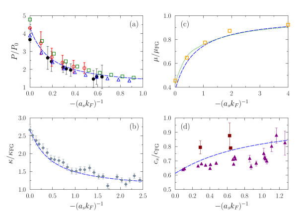
Figure 1: The pressure (a), the isothermal compressibility (b), the chemical potential (c) and the sound velocity (d) as function of $-(a_{s}k_{F})^{-1}$ obtained from the functional (1) assuming $r_{e}=0$ (blue long dashed line). The quantity $P_{0}$ is defined as $P_{0}=(\mu/\mu_{\rm FG})^{5/3}P_{\rm FG}$. For comparison, different experimental data or theoretical estimates are shown: (a) black filled circles are data from Nav10 , QMC calculations from Bul08 (red open circles), results obtained from a Noziére-Schmitt-Rink approximation (blue open triangles) Hu06 or with Green-function method (De Dominicis-Martin formalism) (green open squares) Hau07 ; (b) gray filled diamonds from Hor16 ; (c) calculation from Pie05 (open orange squares), and the green dotted line is obtained from the best fit to the QMC calculations Ast04 (data taken from figure 3 of Hu06 ); (d) brown filled squares and purple triangles are data respectively from Wei15 and Jos07 .

III.1 Ground state thermodynamical properties

Thermodynamical properties of atomic gases have been extensively studied both at zero and finite temperature Zwe11 . In the present work, we concentrate on the zero-temperature limit. Starting from a density functional approach, we summarize below the expression of selected quantities as a function of derivatives of the energy in homogeneous systems:

• Pressure:

  $$P=\left.{\rho^{2}}\frac{\partial E/N}{\partial\rho}\right|_{N}.$$ (3)

• Compressibility:

  $$\kappa=\frac{1}{\rho}\left(\left.\frac{\partial P}{\partial\rho}\right|_{N}\right)^{-1},$$ (4)

  leading to

  $$\frac{1}{\rho\kappa}=\frac{2P}{\rho}+\rho^{2}\left.\frac{\partial^{2}E/N}{\partial\rho^{2}}\right|_{N}.$$ (5)

• Chemical potential:

  $$\mu = \left.\frac{\partial E}{\partial N}\right|_{V}=\left.\frac{\partial\rho E/N}{\partial\rho}\right|_{V}=\frac{E}{N}+\rho\left.\frac{\partial E/N}{\partial\rho}\right|_{V}$$ (6)

  $$= \frac{E}{N}+\frac{P}{\rho}.$$

• Sound velocity and adiabatic index: From the above quantities one can deduce the sound velocity $c_{s}^{2}=(m\rho\kappa)^{-1}$ and the adiabatic index

  $$\Gamma=\left.\frac{\rho}{P}\frac{\partial P}{\partial\rho}\right|_{N}=\frac{1}{\kappa P}.$$ (7)

Alternative expressions can be obtained using directly the quantity $\xi$ introduced in Eq. (1) and its derivatives with respect to the Fermi momentum. These expressions are listed in table 2 together with specific limits obtained at or close to unitarity.

In the following, we will normalize these thermodynamical quantities to their corresponding values for the free FG case, given by:

$$P_{\mathrm{FG}} \equiv \frac{2}{3}\rho\mathcal{E}_{\mathrm{FG}},~{}~{}~{}\frac{1}{\kappa_{\mathrm{FG}}}\equiv\frac{10}{9}\rho\mathcal{E}_{\mathrm{FG}},$$

$$c_{\mathrm{FG}}^{2} \equiv \frac{10}{9m}\mathcal{E}_{\mathrm{FG}},~{}~{}~{}\mu_{\mathrm{FG}}\equiv\frac{5}{3}\mathcal{E}_{\mathrm{FG}}=\frac{\hbar^{2}k_{F}^{2}}{2m},$$

where $\mathcal{E}_{\mathrm{FG}}$ is defined in equation (2).

Thermodynamical quantities obtained using the simple functional for $r_{e}=0$ and arbitrary large negative scattering length are compared in Fig. 1 with various experimental observations and/or theoretical estimates. Not surprisingly, the functional reproduces the unitary limit since it has explicitly been adjusted to reproduce the Bertsch parameter $\xi_{0}$. We see that, despite its simplicity and the fact that the functional only depends on $\xi_{0}$, it is able to reproduce rather well the thermodynamics of Fermi–gas away from unitarity. It should be noted that none of the Taylor expansions in $(a_{s}k_{F})$ or $(a_{s}k_{F})^{-1}$ would be able to reproduce these quantities from very low to very high densities, as illustrated in Fig. 2 for the pressure. Similar behavior is obtained for the other quantities shown in Fig. 1.

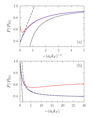
Figure 2: Pressure as a function of $-(a_{s}k_{F})^{-1}$ (a) or as a function of $-(a_{s}k_{F})$ (b) obtained from the functional (1) assuming $r_{e}=0$ fm (blue long dashed line). For comparison, the black short dashed and the black short dot-dashed lines correspond to the Taylor expansion to first order in $(a_{s}k_{F})$ or to first order in $(a_{s}k_{F})^{-1}$ respectively. The red solid line corresponds to the neutron matter case assuming $r_{e}=2.716$ fm. In both cases, $a_{s}=-18.9$ fm.

III.2 Non-zero effective range effect

Figure 3: The pressure [$X=P$] (blue solid line), chemical potential [$X=\mu$] (red dashed line) and inverse compressibility [$X=1/\kappa$] (green dot-dashed line) obtained at unitarity using the functional (8) as a function of $(r_{e}k_{F})$. The arrow indicates the unitary limit for $r_{e}=0$.

In Fig. 2, we also show an example of evolution of thermodynamical quantities for non-zero effective range relevant for neutron matter. In the present functional, the effect of $r_{e}$ is mainly visible at large $(a_{s}k_{F})$ values, i.e. close to unitarity. To illustrate the dependence with $r_{e}$, we consider the strict unitary limit. In that case, the $\xi$ function depends only on $(r_{e}k_{F})$ and we deduce:

$$\xi(a_{s}k_{F}\rightarrow-\infty,r_{e}k_{F}) = \xi_{0}+\frac{\eta_{e}^{2}(r_{e}k_{F})}{\eta_{e}-\delta_{e}(r_{e}k_{F})},$$ (8)

from which all thermodynamical quantities can be calculated. The effect of the effective range is predicted to increase the apparent Bertsch parameter leading also to an increase of the thermodynamical quantities at unitarity. This is illustrated in Fig. 3 for the pressure, the chemical potential and the inverse of the compressibility. We see in particular that the maximal value of $\xi$ at unitarity is $\xi_{0}-\eta_{e}^{2}/\delta_{e}=0.66$ which is almost twice the value of $\xi_{0}$ and therefore might be significant.

III.3 Ground state thermodynamics of neutron matter

We have extended the above study to the case of neutron matter for which we anticipate important influence of the effective range $r_{e}$ as well as eventually of higher order channels contributions when the density increases. The different thermodynamical quantities obtained using the functional (1) with realistic values of the low energy constant $a_{s}$ and $r_{e}$ are shown in Fig. 4. While at very low density the different quantities are only slightly affected by effective range, we indeed observe at densities of interest in the nuclear context, i.e. $\rho\simeq 0.05-0.15$ fm^-3, differences with the cold atom case.

Figure 4: The pressure (a), the inverse of the compressibility (b), the chemical potential (c) and the sound velocity (d) obtained in neutron matter as function of $-(a_{s}k_{F})$ using the functional (1) (red solid line). The case with $r_{e}=0$ (cold atom reference) is displayed with blue dashed line. The green dot-dashed line corresponds to the result obtain by adding to the functional the leading order contribution of the $p$-wave (see text). In this figure, we use $a_{s}=18.9$ fm and $r_{e}=2.716$ fm so that $-(a_{s}k_{F})=10$, $20$ and $30$ correspond respectively to $\rho=0.005$, $0.040$ and $0.135$ fm^-3.

IV Static response in Fermi liquids

Some of the ground state quantities discussed above are directly connected to the static response of the Fermi system to an external field. In general, the static response provides interesting insight about the complex internal reorganization in strongly interacting Fermi liquids Pin66 ; Kit05 . The static or dynamical responses have been the subject of extensive studies in the context of nuclear density functional theory Gar92 ; Pas12 ; Pas12-b ; Pas12-c ; Pas15 especially those based on the Skyrme EDF. As we will see, in the latter case, the static response strongly depends on the set of parameters used in the Skyrme EDF. Recently, the ab-initio static response of neutron matter has been obtained using AFDMC for the first time in Refs. Bur16 ; Bur17 giving strong constraints on nuclear EDF. One surprising result is that the static response is very close to the free FG response. Below we make a detailed discussion on the static response obtained using the functional (1). Since the methodology to obtain the static response is already well documented Pin66 ; Kit05 , we only give the important equations used thorough the article.

IV.1 Generalities on static response

Let us consider a system described by a many-body Hamiltonian $\hat{H}$. A static external one-body field, denoted by $V_{\rm ext}$ is applied to the system leading to a change of its properties. The static response, denoted by $\chi$ contains the information on how the one-body density and total energy vary with the external field. $\chi$ is defined through:

$$\delta\rho({\mathbf{r}}) = \int d^{3}{\mathbf{r}}^{\prime}{\chi}({\mathbf{r}}-{\mathbf{r}}^{\prime})V_{\rm ext}({\mathbf{r}}^{\prime}),$$ (9)

where $\delta\rho({\mathbf{r}})=\rho({\mathbf{r}})-\rho_{0}$, $\rho({\mathbf{r}})$ and $\rho_{0}$ being respectively the local one-body density and the equilibrium density of the uniform system in its ground state. From this, one can express the static response formally as

$$\chi({\mathbf{r}}-{\mathbf{r}}^{\prime}) = \left(\frac{\delta\rho({\mathbf{r}})}{\delta V_{\rm ext}({\mathbf{r}}^{\prime})}\right).$$ (10)

Performing the Fourier transform of Eq. (9), we simply have:

$$\delta\rho({\mathbf{q}}) = {\chi}({\mathbf{q}})V_{\rm ext}({\mathbf{q}}).$$ (11)

Following Refs. Bur16 ; Bur17 , we assume $V_{\rm ext}({\mathbf{r}})=2\sum_{\mathbf{q}}v_{q}\cos({\mathbf{q}}\!\cdot\!{\mathbf{r}})$. The Fourier transform of $V_{\rm ext}$ at ${\mathbf{q}}$ is then simply a constant and we have for the energy:

$$E({\mathbf{q}}) = E_{0}+\frac{\chi(q)}{\rho_{0}}v^{2}_{q}+\cdots$$ (12)

The static response function is directly linked to the compressibility $\kappa$ discussed above due to the asymptotic relationship:

$$\lim_{q\to 0}\chi(q)=-\rho^{2}\kappa.$$ (13)

The function $\chi(q)$ or its dynamical equivalent has been extensively studied for the Skyrme EDF Pas15 . In Fig. 5, we give examples of results obtained using different sets of Skyrme parameters and compared them with the AFDMC results of Refs. Bur16 ; Bur17 . It is clear from this figure that there is a large dispersion in the Skyrme EDF response depending on the parameter sets. Such a dispersion is not surprising since it is well known that the neutron equation of state is weakly constrained in Skyrme EDF (see for instance Bro00 ). In all cases, even if the Skyrme EDF gives reasonable neutron matter EOS, significant difference is observed with the exact AFDMC result for all ranges of $q/k_{F}$. This figure also illustrates the fact that the exact result is very close to the free Fermi–gas response.

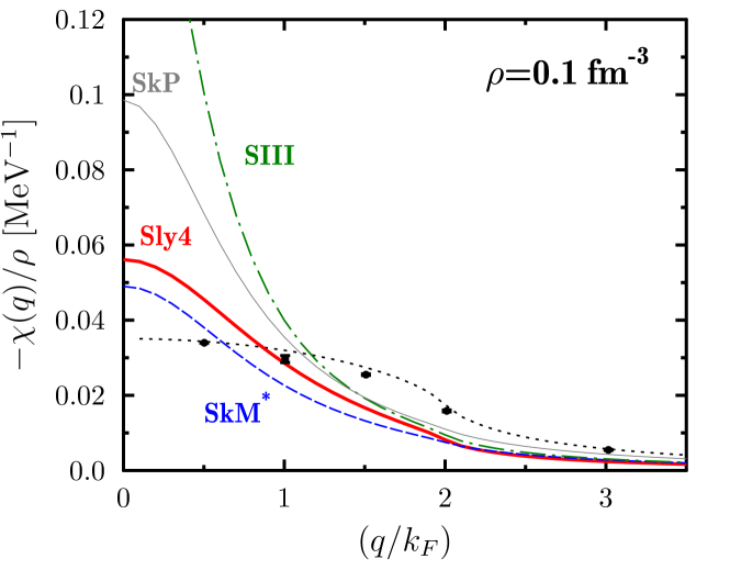
Figure 5: Static response of neutron matter at density $\rho=0.1$ fm^-3 obtained with the Skyrme EDF using the Sly4 (red thick solid line), SkM^∗ (blue dashed line), SkP (gray thin solid line) and SIII (green dot-dashed line) sets of Skyrme parameters (see Mey03 for their values). Note that the EDF results are obtained by neglecting the spin–orbit term in the functional. Adding the spin–orbit contribution does not change significantly the result. The black circles (with errorbars) are those of Ref. Bur17 while the black dotted line is the free Fermi–gas static response.

An important ingredient of the response in Skyrme EDF is the evolution of the effective mass as a function of the density. Such evolution is shown in Fig. 6(a). Again, large differences are observed between the different sets of Skyrme EDF. We also show for comparison, the effective mass obtained in neutron matter using alternative many-body techniques. In these cases, the deduced effective mass are closer to the bare mass but still significantly differ with each other.

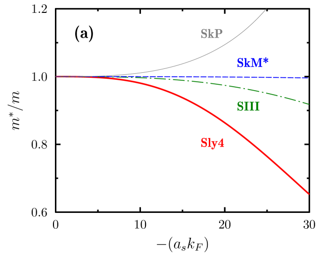
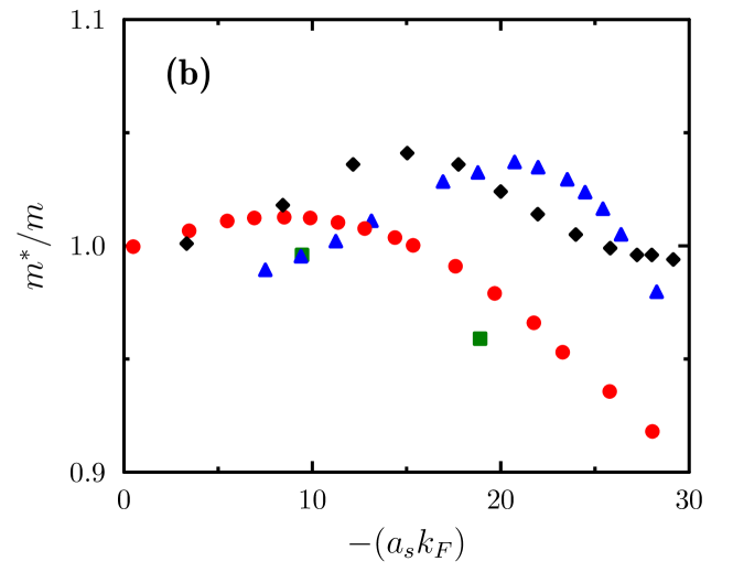
Figure 6: (a) Evolution of the effective mass $m^{*}/m$ in neutron matter as a function of $-(a_{s}k_{F})$ (with $a_{s}=-18.9$ fm) using Skyrme EDF for the set of parameters used in Fig. 5 with the same lines convention. (b) Evolution of the effective mass in neutron matter deduced from selected many-body calculations: blue triangles Sch03 , red circles Wam93 , green squares Fri81 , black diamonds Dri14 .

In the absence of clear guidance for the effective mass behavior, we simply assume below that $m^{*}/m=1$. Then, the calculation of the static response within the density functional approach reduces to

$$\chi(q) = \frac{\chi_{0}(q)}{1-G(\rho)\chi_{0}(q)},$$ (14)

where $\chi_{0}(q)$ is the response of the free gas given in term of the Lindhard function (dashed line in Fig. 5)

$$\chi_{0}({q}) = -\frac{mk_{F}}{2\pi^{2}\hbar^{2}}\left[1+\frac{k_{F}}{q}\left(1-\left(\frac{q}{2k_{F}}\right)^{2}\right)\ln\left|\frac{q+2k_{F}}{q-2k_{F}}\right|\right],$$ (15)

$$\equiv -\frac{mk_{F}}{\pi^{2}\hbar^{2}}f(q/k_{F}).$$

The density-dependent coefficient $G(\rho)$ is obtained from the second derivative of the energy density after subtraction of the kinetic contribution. Explicitly, the energy can be rewritten as an integral over the energy density through:

$$E = \int\left\{{\cal K}({\mathbf{r}})+{\cal V}({\mathbf{r}})\right\}d^{3}{\mathbf{r}},$$

where ${\cal K}$ is the kinetic energy density and ${\cal V}$ is the potential energy density. For uniform system, $G(\rho)$ is given by:

$$G(\rho) = \left(\frac{\partial^{2}{\cal V}}{\partial^{2}\rho}\right),$$ (16)

that could again eventually be transformed as partial derivatives with respect to $k_{F}$.

IV.1.1 Static response in unitary gas

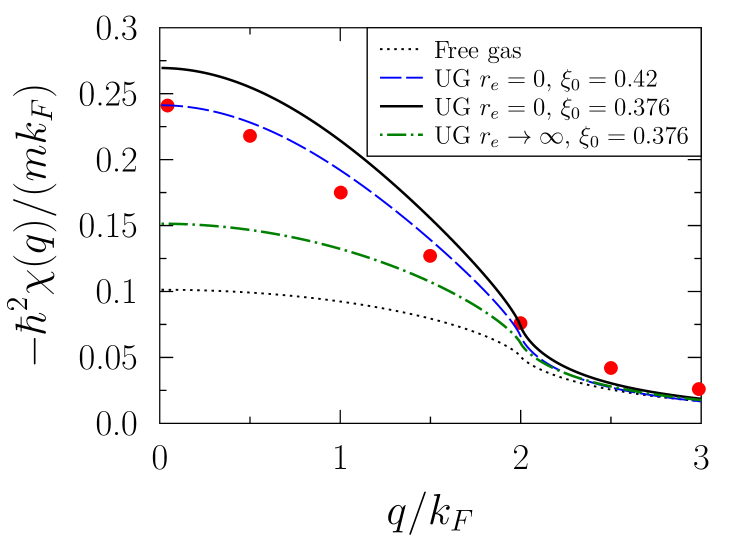
Figure 7: Static response of unitary gas (UG) obtained with the functional (8) assuming $r_{e}=0$ (black solid line) or $r_{e}\rightarrow+\infty$ (green dot-dashed line). The latter case corresponds to the maximum effect induced by $r_{e}$ and corresponds to an effective Bertsch parameter equal to $0.66$. The free Fermi–gas response (black dotted line) is also shown as a reference. For comparison, the red filled circles corresponds to the static response at unitarity obtained in ref. For14 using the SLDA where a slightly different value of the Bertsch parameter $\xi_{0}=0.42$ was assumed. For completeness, we also show (blue dashed line) the UG result obtained with (8) for $\xi_{0}=0.42$.

We consider first the strict unitary gas limit with $r_{e}=0$. In this case, we have

$${\cal V}(\rho)=\frac{3}{5}\frac{\hbar^{2}}{2m}(3\pi)^{2/3}\rho^{5/3}(\xi_{0}-1).$$ (17)

Using this expression, we obtain:

$$\chi(q) = -\frac{mk_{F}}{\pi^{2}\hbar^{2}}\frac{f(q/k_{F})}{\left[1+(\xi_{0}-1)f(q/k_{F})\right]}$$ (18)

where $f(q/k_{F})$ is defined through Eq. (15). In particular, we see immediately that $\chi(0)=\chi_{0}(0)/\xi_{0}$, with $\chi_{0}(0)=-\frac{mk_{F}}{\pi^{2}\hbar^{2}}\displaystyle$ that is a direct consequence of the property (13) and of the fact that $\kappa_{\rm FG}/\kappa=\xi_{0}$ in unitary gas (see table 2).

The full static response is shown in Fig. 7 and compared to the result obtained in Ref. For14 using the Superfluid Local Density Approximation (SLDA) proposed in Refs Bul07a ; Mag09 . The static response calculated with the functional (15) perfectly matches the SLDA result when the Bertsch parameter is artificially increased to match the one used in the SLDA. Note that, the SLDA assumed a significant contribution from the effective mass and account also for superfluid effects, which is not the case in the present work. Therefore, an indirect conclusion is that the static response for UG does not seem to be significantly influenced in particular by superfluidity. We would like to insist on the fact that this is most probably specific to the response to a static field. Indeed, due to superfluidity, the dynamical response will present a low energy mode, the so-called Bogoliubov-Anderson mode that has been studied for instance in Ast14 . The superfluid nature of Fermi gas at unitarity has been unambiguously directly probed by the presence of lattice of quantized vortices in Ref. Zwe05 .

Note finally that the matching of the static response obtained with the two functional approach observed in Fig. 7 is an interesting information but it does not mean that the static response is the correct one at unitarity. A comparison with an exact calculation would be desirable (see also discussion in section VI).

The effect of $r_{e}$ at unitarity can be studied using the generalization of Eq. (17):

$${\cal V}(\rho)=E_{\rm FG}(\rho)[\xi(r_{e}k_{F})-1],$$

where $\xi(r_{e}k_{F})$ is given by Eq. (8). The predicted influence of $r_{e}$ is illustrated in Fig. 7. The effective range induces a global reduction of $\chi(q)$. The maximum effect is achieved by considering the limit $r_{e}\rightarrow+\infty$ (green dot dashed curve).

IV.2 Static response in neutron matter

The neutron matter differs from the unitary gas by a finite value of the scattering length as well as significant effect of the effective range even at rather low density Lac17 . When the density increases, it is also anticipated that higher partial waves of the interaction contribute. Since our aim is to compare with the recent result of ref. Bur17 where the AV8 interaction has been used, we use the functional (1) using the AV8 values for the different parameters: $a_{s}=-19.295~{}\mathrm{fm}$ and $r_{e}=2.716~{}\mathrm{fm}$. We note that, the functional (1) reproduces well the energy for rather low densities $\rho<0.02-0.03$ fm^-3 Lac17 while the static responses of Ref. Bur17 have been obtained for $\rho=0.04$ and $0.1$ fm^-3 which is not optimal for the comparison.

We show in Fig. 8 the static response obtained from the functional (1) and compare it to the AFDMC results of Refs. Bur16 ; Bur17 . While slightly overestimated, especially in the highest density considered, we first observe that the new functional is in much better agreement than the empirical functional considered in Fig. 5. For the considered densities, as underlined in Ref. Lac17 , the functional (1) can be accurately replaced by its unitary gas limit, i.e. taking $-(a_{s}k_{F})^{-1}=0$. Indeed, replacing $\xi$ entering in the full functional by $\xi$ given by Eq. (8) leads almost to the same total energy and static response (not shown). Still, the static response obtained by neglecting the $r_{e}$ effect is rather far from the static response obtained with the physical $r_{e}$, underlying the key role played by the effective range.

Following Ref. Lac17 , we also study the possible influence of the $p$-wave contribution by adding simply its leading order contribution to the energy, that is

$$\frac{E_{p}}{E_{\rm FG}} = \frac{1}{\pi}(a_{p}k_{F})^{3}.$$

The results are displayed in Fig. 8. We see that the $p$-wave term, treated simply by its leading order contribution does contributes to the static response and, most importantly, the result is very close to the ab-initio one. For the sake of completeness, we also report in Fig. 4 the different thermodynamical quantities obtained by including the $p$-wave term. However the contribution should only be taken here as indicative. As noted already in Ref. Lac17 , the inclusion of the leading term of the $p$-wave, produces a rather large, most probably unphysical, contributions to the different quantities and when density increases one should a priori properly account for the $p$-wave contribution accounting from the re-summation of the s-wave effect as illustrated in Ref. Sch05 . This is out of the scope of the present work.

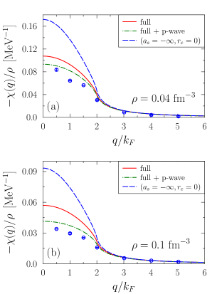
Figure 8: Static response function obtained with the functional (1) as function of $q/k_{F}$ for (a) $\rho=0.04~{}\mathrm{fm^{-3}}$ and (b) $\rho=0.1~{}\mathrm{fm^{-3}}$. The blue dashed line and red solid line corresponds respectively to the UG case (cold atom reference) and $r_{e}=2.716~{}\mathrm{fm}$ (neutron matter case). Note that at the density considered, the UG case cannot be distinguished from the neutron matter assuming $r_{e}=0$. At both densities, the AFDMC results of Refs. Bur16 ; Bur17 are shown with blue open circles. The green dot-dashed line finally display the result obtained by adding the $p$-wave contribution to the functional (1). Consistently with the use of the AV8 interaction in the AFDMC calculation, we use a value $a^{3}_{p}=0.0916$ fm for the $p$-wave scattering volume.

Finally, to systematically quantify the effects of finite $a_{s}$, influence of $r_{e}$ and $p$-wave, we have reproduced the Fig. 15 of Ref. Bur17 where the normalized response function is shown for different densities (Fig. 9). In this figure, we can clearly see the importance of the effective range and to a lesser extend, the slightly smaller effect of the $p$-wave. Still the free Fermi–gas case is the one that best reproduces the AFDMC result. However, this is most probably accidental in view of the strong interaction at play in nuclear systems.

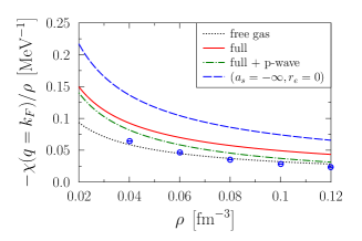
Figure 9: Evolution of the normalized static response as a function of density for $q=k_{F}$ (same as Fig. 15 of Ref. Bur17 ). The AFDMC results of Ref. Bur17 is shown by blue open circles. The result of the functional (1) with $r_{e}=2.176$ fm and $r_{e}=0$ fm are shown by red solid and blue dashed line respectively. The result obtained by adding the $p$-wave contribution to the functional is shown by green dot-dashed line. The black dotted line corresponds to the free Fermi–gas limit.

We finally would like to mention that we are unable with the present density functional to reproduce the strong increase of the response function as $q\rightarrow 0$ that is observed in the AFDMC. This limit is directly connected to the compressibility (see Eq. (13)). The compressibilities predicted by our EDF are $\rho\kappa=0.108~{}\mathrm{MeV}$ and $\rho\kappa=0.057~{}\mathrm{MeV}$ at $\rho=0.04~{}\mathrm{fm}^{-3}$ and $\rho=0.1~{}\mathrm{fm}^{-3}$ respectively. These values are lower than those reported in Ref. Bur17 which are respectively $\rho\kappa=0.19~{}\mathrm{MeV}$ and $\rho\kappa=0.089~{}\mathrm{MeV}$ at $\rho=0.04~{}\mathrm{fm}^{-3}$ and $\rho=0.1~{}\mathrm{fm}^{-3}$.

V Collective response in the hydrodynamical regime

We conclude this work by using previous results to study the collective excitations in cold atoms and neutron matter in the hydrodynamical regime. For boson systems, the hydrodynamical regime is well documented Lip08 ; Str96 . Similar technique can be applied to fermionic superfluid systems. Note that here, we do not include explicitly the pairing correlations through the anomalous density. However, the fact that we properly describe the total energy of cold atoms, is an indication that pairing effect is accounted for in some way. For superfluid Fermi system, the hydrodynamical regime is justified when the collective frequency is below the energy necessary to break a Cooper pair (see for instance Bul05 . Our aim is to study the dynamical response of a system confined in a trap, describe by an external potential $U({\mathbf{r}})$. At equilibrium, the external field is counterbalanced by the internal pressure leading to the equilibrium equation:

$$\nabla^{2}P({\mathbf{r}}) = -\frac{1}{m}\nabla\left[\rho_{0}({\mathbf{r}}).\nabla U({\mathbf{r}})\right],$$ (19)

where $\rho_{0}$ denotes the equilibrium density while $P$ is the pressure at equilibrium given by Eq. (3). We now consider small amplitude oscillations around equilibrium such that $\rho({\mathbf{r}},t)=\rho_{0}({\mathbf{r}})+\delta\rho({\mathbf{r}},t)$ with $\delta\rho({\mathbf{r}},t)=\rho_{1}e^{i\omega t}+{\rm h.c.}$. The linearization of the hydrodynamical equation leads to the equation:

$$\omega^{2}\rho_{1}({\bf r})=-\frac{1}{m}\nabla\cdot\left[\rho_{1}({\bf r})\nabla U({\bf r})\right]-\nabla^{2}\left[c_{0}^{2}({\bf r})\rho_{1}({\bf r})\right],$$ (20)

where $c^{2}_{0}({\bf r})$ is the local sound velocity defined through: $mc^{2}_{0}({\bf r})\equiv dP({\mathbf{r}})/d\rho_{0}({\mathbf{r}})$. This equation has been used in several works to study collective oscillations in Fermi–gas around unitarity Bul05 ; Str96 ; Hei04 ; Adh08 . Below we extend these studies by considering possible effect of non-zero $r_{e}$ and by going from cold atoms to neutron matter.

V.1 Adiabatic index in cold atoms and neutron matter

For the sake of simplicity, we assume that the system has a polytropic equation of state, i.e. that we simply have:

$$P({\bf r})\propto\rho_{0}^{\Gamma}({\bf r}),$$ (21)

where $\Gamma$ is the adiabatic index in the center of the trapping potential. As in infinite system, we have the relation $\Gamma=(\kappa_{c}P_{c})^{-1}$ where $P_{c}$ and $\kappa_{c}$ denote the pressure and the compressibility in the center of the trapping potential at equilibrium given by Eqs. (3) and (5). The quantity $\Gamma$ has been studied in cold atoms for varying $-(a_{s}k_{F})$ in Ref. Cha04 . For vanishing $r_{e}$, it is know that $\Gamma\rightarrow 5/3$ both in the unitary limit and in the low density regime. For UG, when $r_{e}$ could not be neglected anymore, using the functional (8), we predict that $\Gamma$ will deviate from $5/3$. The dependence of $\Gamma$ with the effective range is shown in Fig. 10. We see that $\Gamma$ first increases and then decreases. In the extreme limit $r_{e}\rightarrow+\infty$, it is possible to show that we again obtain $\Gamma\rightarrow 5/3$.

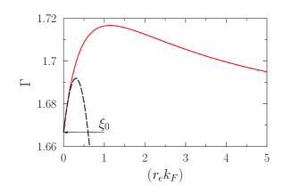
Figure 10: Evolution of the non-adiabatic index $\Gamma$ at unitarity (red solid line) deduced from the functional (8) as a function of $(r_{e}k_{F})$. The arrow indicates the unitary limit for $r_{e}=0$. For comparison, the black short dashed line corresponds to the Taylor expansion of $\xi$ to second order in $(r_{e}k_{F})$.

More generally, we illustrate the dependence of $\Gamma$ obtained with or without effective range effects in Fig. 11 for low energy constants taken from neutron matter.

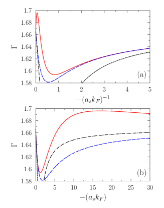
Figure 11: Adiabatic index as a function of $-(a_{s}k_{F})^{-1}$ (a) or as a function of $-(a_{s}k_{F})$ (b) obtained from the functional (1) assuming $r_{e}=0$ fm (blue long dashed line). For comparison, the black short dashed and the black short dot-dashed lines correspond to the Taylor expansion to first order in $(a_{s}k_{F})$ or to first order in $(a_{s}k_{F})^{-1}$ respectively. The red solid line corresponds to the neutron matter case assuming $r_{e}=2.716$ fm. In both cases, $a_{s}=-18.9$ fm.

For $r_{e}=0$, we qualitatively and quantitatively reproduce the result of Ref. Cha04 with the presence of a minimum in $\Gamma$ for $-2.5<(a_{s}k_{F})<0$. While the minimum persists for non-vanishing $r_{e}$, we observe that it is slightly shifted to lower values of $|a_{s}k_{F}|$. Overall, we see that $r_{e}$ significantly affects the evolution of $\Gamma$ that now presents a maximum and approaches $\Gamma=5/3$ from above as $-(a_{s}k_{F})\rightarrow+\infty$.

V.2 Collective frequencies in anisotropic trap

As shown in Ref. Hei04 , assuming polytropic equation of state leads to rather simple expression of the collective oscillations in deformed systems. More precisely, we consider here a system confined in an anisotropic trap

$$U({\bf r})=\frac{m}{2}\omega_{0}^{2}\left(x^{2}+y^{2}+\lambda^{2}z^{2}\right),$$ (22)

where $\lambda$ gives a measure of the anisotropy, with $\lambda<1$ and $\lambda>1$ for prolate or oblate deformations respectively. Then Heiselberg Hei04 has obtained analytical expression for the collective frequencies along the elongation axis or perpendicular to the elongation axis. This collective axis are called below axial or radial collective frequencies and are denoted by $\omega_{\rm ax}$ and $\omega_{\rm rad}$ respectively.

For prolate deformation with $\lambda\ll 1$, the two frequencies are given by:

$$\frac{\omega_{\rm ax}^{p}}{\omega_{0}} = \lambda\sqrt{3-\frac{1}{\Gamma}},$$ (23)

$$\frac{\omega_{\rm rad}^{p}}{\omega_{0}} = \sqrt{2\Gamma},$$ (24)

while in the oblate limit $\lambda\gg 1$, we have:

$$\frac{\omega_{\rm ax}^{o}}{\omega_{0}} = \lambda\sqrt{\Gamma+1},$$ (25)

$$\frac{\omega_{\rm rad}^{o}}{\omega_{0}} = \sqrt{\frac{6\Gamma-2}{\Gamma+1}}.$$ (26)

Note that for $\lambda=1$ we recover results obtained for isotropic trap Coz03 ; Hei04 . We then see that a change in $\Gamma$ will be reflected by a change in the axial and radial collective frequencies.

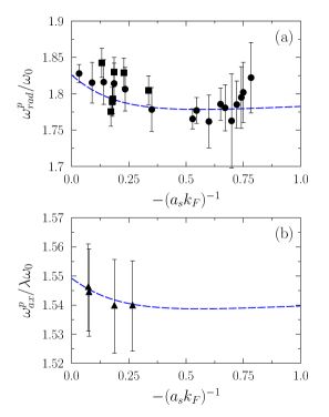
Figure 12: $\omega^{p}_{rad}/\omega_{0}$ (a) and $\omega^{p}_{ax}/(\lambda\omega_{0})$ (b) as function of $-(a_{s}k_{F})^{-1}$ obtained with the functional (1) with $r_{e}=0$ (blue dashed line). The symbols are experimental data: triangles from Bar04a , circles from Kin04b and squares from Kin04a . (All data sets are taken from Fig. 3 of Ref. Man05a )

The collective response of cold atoms with possible anisotropy for the trapping potential has attracted much attention in the last decades. The experimental axial and radial frequencies are shown at or around unitarity for prolate shapes in Fig. 12. At unitarity ($\Gamma=5/3$), we expect to have $\omega_{\rm ax}^{p}/(\lambda\omega_{0})=\sqrt{12/5}\simeq 1.549$ and $\omega_{\rm rad}^{p}/\omega_{0}=\sqrt{10/3}\simeq 1.826$ that seems coherent with the observations. In Fig. 12, we also display the results of Eqs. (24) and (23). using the adiabatic index obtained from the functional (1) with $r_{e}=0$. We see that the estimated collective frequencies are consistent with the observation in cold atoms. We then investigate the possible effect of $r_{e}$ in the strict unitary regime in Fig. 13. In this case, the $\Gamma$ that is used in Eqs. (24-23) is displayed in Fig. 10. We see a rather weak dependence of the collective frequencies with $r_{e}$.

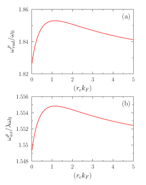
Figure 13: $\omega^{p}_{\rm rad}/\omega_{0}$ (a) and $\omega^{p}_{\rm ax}/(\lambda\omega_{0})$ (b) as function of $(r_{e}k_{F})$ obtained with the functional (1) at unitarity $(a_{s}k_{F})^{-1}=0$.

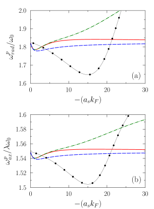
Figure 14: $\omega^{p}_{\rm rad}/\omega_{0}$ (resp. $\omega^{p}_{\rm ax}/\omega_{0}$) as a function of $-(a_{s}k_{F})$ (a) (resp. (b)) obtained in neutron matter using $a_{s}=-18.9~{}\mathrm{fm}$ and $r_{e}=2.716~{}\mathrm{fm}$ (red solid line) in the functional (1) while the blue long-dashed line corresponds to the result obtained with $r_{e}=0$. For comparison, we also show the result of the Skyrme Sly5 parameter sets (black filled circles) and the result obtained by adding to the functional the leading order $p$-wave contribution (green dot-dashed line).

We finally display in Fig. 14 the collective frequencies obtained for confined neutron systems in an anisotropic trap. As far as we know, the present work is the first attempt to determine this particular quantity neutronic systems. Collective frequencies obtained with the functional are compared with the case of cold atoms and with the result of the empirical Skyrme EDF with Sly5 sets of parameter. It is first noted that collective frequencies are strongly dependent on the used functional and therefore the dynamical collective frequencies of trapped neutron is a stringent test of the functional used. We finally would like to mention that the collective frequencies are calculated here assuming that the local density approximation is valid. However, the collective frequencies might be affected by the introduction of gradients of the densities as it is usually done in more empirical functional like Skyrme ones. In addition, we predict rather large differences between neutron matter and cold atoms that are due to effective range effects as well as higher order channels like $p$-wave when the density increases.

VI Critical discussion on the role of pairing

In the present article, we focused our attention on the static response of doubly degenerated Fermi liquid with anomalously large $s$-wave scattering length. We have seen that, assuming that the effective mass is approximately equal to the bare mass and neglecting possible effect of superfluidity, our functional can describe reasonably the ground state thermodynamical quantities close or at unitarity in cold atoms and can give interesting insight for the static response of neutron matter. The comparison is less favorable when performing the full dynamical response. Using the same assumptions as for the static response, we also calculated the dynamical response of the system to a small oscillating external perturbation $V_{\rm ext}(\mathbf{r},t)$ with varying frequency $\omega$. The dynamical response function $\chi(q,\omega)$ then generalizes the static response Gar92 ; Pas15 that is obtained as the specific case $\omega=0$.

One then defines the dynamical structure function $S(q,\omega)$ through:

$$S(q,\omega)=-\frac{1}{\pi}\Im\left[\chi(q,\omega)\right].$$ (27)

While the static response function has not been directly obtained in UG, its dynamical structure function has been studied both experimentally and theoretically in Refs Hoi12 ; Ast14 .

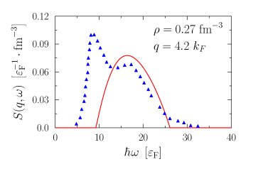
Figure 15: Dynamical structure function at unitarity obtained from the functional (1) (red solid line) compared to the experimental results of Ref. Hoi12 (blue triangles). $\varepsilon_{F}=\hbar^{2}k_{F}^{2}/2m$ is the Fermi energy.

The experimental structure function obtained in Ref. Hoi12 is compared to the response obtained with the functional (1) in Fig. 15. The experimental response presents two separated peaks. We obviously see that the dynamical response obtained with our functional is able approximately to reproduce the second peak but completely miss the collective mode at low energy. This mode is indeed due to superfluidity leading to the so-called Bogoliubov-Anderson mode, that seems difficult to describe without explicitly using a quasi-particle picture. As shown in Ref. Zou16 using the RPA approach with the SLDA, accounting for superfluidity leads back to the proper low energy collective modes that reproduces qualitatively the observation. As shown above, many aspects can be properly reproduced in cold atoms without explicitly introducing superfluidity. However, the dynamical response clearly points out the necessity in the near future to explicitly include the anomalous density in the description.

One can also obtain the static structure function $\bar{S}(q)$, defined through

$$\bar{S}(q)=\int d\omega S(q,\omega),$$

that has been obtained for UG in Ref. Hoi13 where it is compared to QMC results (see also Ref. Car14 ). We show in Fig. 16 a comparison of the static structure factor obtain with the functional with the Monte-Carlo result of Ref. Car14 .

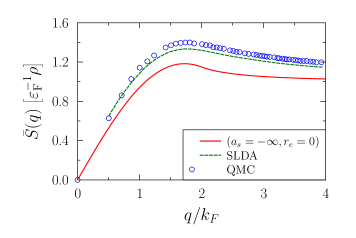
Figure 16: Static structure function obtained with the functional (with $r_{e}=0$) (red solid line) as a function of $q/k_{F}$ compared to the Diffusion Monte-Carlo result of Ref. Car14 (blue circles). For comparison, we also show the result obtained in Ref. Zou16 with the SLDA (green dashed line).

Not surprisingly, due to the missing peak at low energy, $\bar{S}(q)$ is underestimated compared to the exact results. Our conclusion, is that for specific aspects like the dynamical response, it will be necessary to improve the functional by allowing $U(1)$ symmetry breaking. The same situation will also happen for neutron matter at very low density. However, in this case, when the density increases pairing gap exponentially decreases. In particular, at densities considered in the DFMC results of Ref. Bur16 ; Bur17 , pairing is expected to not affect the static response.

VII Conclusion

In the present work, we make a detailed analysis of thermodynamical ground-state properties of both cold atoms and neutron matter starting from the new density functional proposed in Refs. Lac16 ; Lac17 . For cold atoms with large negative $s$-wave scattering length and with negligible effective range effects, thermodynamical quantities like the pressure, the chemical potential, the compressibility and zero sound are very well reproduced. We further analyze the possible influence of the effective range at and away from the unitary gas limit. The inclusion of effective range is the first step towards the proper description of neutron matter. The difference between ground-state thermodynamical properties in UG and neutron matter are quantified.

The thermodynamical quantities, and more specifically the compressibility are connected to the static response of Fermi liquids to an external constraint for which exact AFDMC exists Bur16 ; Bur17 . The exact static response is obtained using the new functional. It is shown to be in much better agreement with AFDMC result than the Skyrme type functional especially at low density.

We finally consider the dynamical collective response in the hydrodynamical regime. In the cold atom case, a reasonable description of radial and axial collective frequency is obtained assuming a polytropic equation of state. Following a similar strategy, we estimate the collective frequencies of neutron drops in anisotropic traps. Important differences are observed between Skyrme empirical functional and the new functional discussed here.

- (1) I. Bloch, J. Dalibard and W. Zwerger, Rev. Mod. Phys. 80, 885 (2008).
- (2) S. Giorgini, L. P. Pitaevskii and S. Stringari Rev. Mod. Phys. 80, 1215 (2008).
- (3) C. Chin, R. Grimm, P. Julienne and E. Tiesinga Rev. Mod. Phys. 82, 1225 (2010).
- (4) W. Zwerger, ed. The BCS-BEC crossover and the unitary Fermi–gas. Vol. 836. Springer Science and Business Media, (2011).
- (5) D. Lacroix, Phys. Rev. A 94, 043614 (2016).
- (6) I. Tews, J. M. Lattimer, A. Ohnishi, E. E. Kolomeitsev, arXiv:1611.07133.
- (7) S. König, H. W. Griesshammer, H.-W. Hammer, and U. van Kolck Phys. Rev. Lett. 118, 202501 (2017).
- (8) J. Carlson, S. Gandolfi and A. Gezerlis, Prog. Theor. Exp. Phys. 2012, 01A209 (2012).
- (9) S. Gandolfi, A. Gezerlis and J. Carlson, Annu. Rev. Nucl. Part. Sci. 65, 303 (2015).
- (10) M. Buraczynski and A. Gezerlis, Phys. Rev. Lett. 116, 152501 (2016).
- (11) M. Buraczynski and A. Gezerlis, Phys. Rev. C 95, 044309 (2017).
- (12) D. Lacroix, A. Boulet, M. Grasso and C. J. Yang, Phys. Rev. C 95, 054306 (2017).
- (13) M. J. H. Ku, A. T. Sommer, L. W. Cheuk, and M. W. Zwierlein, Science 335, 563 (2012).
- (14) M. M. Forbes, S. Gandolfi and A. Gezerlis, Phys. Rev. A 86, 053603 (2012).
- (15) T.D. Lee and C.N. Yang, Phys. Rev. 105, 1119 (1957).
- (16) R. F. Bishop, Ann. Phys. 77, 106 (1973).
- (17) S. Tan, Ann. Phys. (N.Y.) 323, 2952 (2008).
- (18) S. Tan, Ann. Phys. (N.Y.) 323, 2971 (2008).
- (19) S. Tan, Ann. Phys. (N.Y.) 323, 2987 (2008).
- (20) S. Y. Chang, V. R. Pandharipande, J. Carlson and K. E. Schmidt, Phys. Rev. A 70, 043602 (2004).
- (21) G. E. Astrakharchik, J. Boronat, J. Casulleras and and S. Giorgini, Phys. Rev. Lett. 93, 200404 (2004).
- (22) N. Navon, S. Nascimbene, F. Chevy and C. Salomon, Science 328, 729 (2010).
- (23) A. Bulgac, J. Drut, P. Magierski, Phys. Rev. A 78, 023625 (2008).
- (24) H. Hu, X. Liu and P. Drummond, Europhys. Lett. 74, 574 (2006).
- (25) R. Haussmann, W. Rantner, S. Cerrito and W. Zwerger, Phys. Rev. A 75, 023610 (2007).
- (26) M. Horikoshi, M. Koashi, H. Tajima, Y. Ohashi and M. Kuwata-Gonokami, Phys. Rev. X 7, 041004 (2017).
- (27) P. Pieri, L. Pisani and G. C. Strinati, Phys. Rev. B 72, 012506 (2005).
- (28) W. Weimer, K. Morgener, V. P. Singh, J. Siegl, K. Hueck, N. Luick, L. Mathey and H. Moritz, Phys. Rev. Lett. 114, 095301 (2015).
- (29) J. Joseph, B. Clancy, L. Luo, J. Kinast, A. Turlapov and J. E. Thomas, Phys. Rev. Lett. 98, 170401 (2007).
- (30) D. Pines and P. Nozières, The Theory of Quantum Liquids, (Benjamin, Reading, 1966), Vol. I.
- (31) C.Kittel, Introduction to solid state physics, (Wiley, 2005).
- (32) C. García-Recio, J. Navarro, Van Giai Nguyen, L.L. Salcedo, Ann. of Phys. , 214, 293 (1992).
- (33) A. Pastore, D. Davesne, Y. Lallouet, M. Martini, K. Bennaceur and J. Meyer, Phys. Rev. C 85, 054317 (2012).
- (34) A. Pastore, M. Martini, V. Buridon, D. Davesne, K. Bennaceur and J. Meyer, Phys. Rev. C 86, 044308 (2012).
- (35) A. Pastore, K. Bennaceur, D. Davesne and J. Meyer, Int. J. Mod. Phys. E 21, 1250040 (2012).
- (36) A. Pastore, D. Davesne and J. Navarro, Phys. Rep. 563, 1 (2015).
- (37) B. Alex Brown, Phys. Rev. Lett. 85, 5296 (2000).
- (38) J. Meyer, Ann. Phys. Fr 23, 1 (2003).
- (39) A. Schwenk, B. Friman and G.E. Brown, Nucl. Phys. A 713, 191 (2003).
- (40) J. Wambach, T.L. Ainsworth, D. Pines, Nucl. Phys. A 555 (1993) 128.
- (41) B. Friedman and V. Pandharipande, Nucl. Phys. A 361, 502 (1981).
- (42) C. Drischler, V. Somà, and A. Schwenk, Phys. Rev. C 89, 025806 (2014).
- (43) M. M. Forbes and R. Sharma, Phys. Rev. A 90, 043638 (2014).
- (44) A. Bulgac, Phys. Rev. A 76, 040502 (2007).
- (45) P. Magierski, G. Wlazlowski, A. Bulgac, and J. E. Drut, Phys. Rev. Lett. 103, 210403 (2009).
- (46) G. E. Astrakharchik, J. Boronat, E. Krotscheck and T. Lichtenegger, J. Phys. Conf. Ser. 529, 012009 (2014).
- (47) M.W. Zwierlein, J.R. Abo-Shaeer, A. Schirotzek, C.H. Schunck, W. Ketterle, Nature 435, 1047 (2005).
- (48) T. Schäfer, C.-W. Kao, and S.R. Cotanch, Nucl. Phys. A 762, 82 (2005).
- (49) E. Lipparini, Modern Many-Particle Physics: Atomic Gases, Quantum Dots and Quantum Fluids, World Scientific Publishing Co Inc, (2008).
- (50) S. Stringari, Phys. Rev. Lett. 77, 2360 (1996).
- (51) Aurel Bulgac and George F. Bertsch, Phys. Rev. Lett. 94, 070401 (2005).
- (52) H. Heiselberg, Phys. Rev. Lett. 93, 040402 (2004).
- (53) S. K. Adhikari, Phys. Rev. A 77, 045602 (2008).
- (54) Marco Cozzini and Sandro Stringari, Phys. Rev. Lett. 91, 070401 (2003)
- (55) M. Bartenstein, A. Altmeyer, S. Riedl, S. Jochim, C. Chin, J. H. Denschlag and R. Grimm, Phys. Rev. Lett. 92, 203201 (2004).
- (56) J. Kinast, A. Turlapov and J. E. Thomas, Phys. Rev. A 70, 051401 (2004).
- (57) J. Kinast, S. L. Hemmer, M. E. Gehm, A. Turlapov and J. E. Thomas, Phys. Rev. Lett. 92, 150402 (2004).
- (58) N. Manini and L. Salasnich, Phys. Rev. A 71, 033625 (2005).
- (59) S. Hoinka, M. Lingham, M. Delehaye and C. J. Vale, Phys. Rev. Lett. bf 109, 050403 (2012).
- (60) P. Zou, F. Dalfovo, R. Sharma, X. J. Liu and H. Hu, New J. Phys. 18, 113044 (2016).
- (61) Sascha Hoinka, Marcus Lingham, Kristian Fenech, Hui Hu, Chris J. Vale, Joaqu n E. Drut, and Stefano Gandolfi Phys. Rev. Lett. 110, 055305 (2013).
- (62) J. Carlson and S. Gandolfi, Phys. Rev. A 90, 011601 (2014)