AMI-CL J0300+2613: a Galactic anomalous-microwave-emission ring masquerading as a galaxy cluster

Abstract

The Arcminute Microkelvin Imager (AMI) carried out a blind survey for galaxy clusters via their Sunyaev–Zel’dovich effect decrements between 2008 and 2011. The first detection, known as AMI-CL J0300+2613, has been reobserved with AMI equipped with a new digital correlator with high dynamic range. The combination of the new AMI data and more recent high-resolution sub-mm and infra-red maps now shows the feature in fact to be a ring of positive dust-correlated Galactic emission, which is likely to be anomalous microwave emission (AME). If so, this is the first completely blind detection of AME at arcminute scales.

1 Introduction

The Arcminute Microkelvin Imager (AMI; Zwart et al. 2008) blind galaxy cluster survey covered $\approx$ 10 deg² of the Northern sky, aiming to detect galaxy clusters via the Sunyaev—Zel’dovich (SZ, Sunyaev & Zeldovich 1972) effect. Data were taken between 2008 and 2010 on both AMI arrays, the Small Array (SA) to observe the extended cluster emission, and the Large Array (LA) to detect, characterise and subtract the confusing radio point sources to high positional accuracy and sensitivity. Only the first detection from the survey, known as AMI-CL J0300+2613, has been published to date in AMI Consortium: Shimwell et al. (2012). This galaxy cluster candidate appeared to be a high-significance, extended, double-peaked SZ source and was also followed up with the Combined Array for Research in Millimeter-wave Astronomy (CARMA; see Muchovej et al. 2007 for more details), with which it was detected with lower significance (AMI Consortium: Shimwell et al., 2013).

Recently, a new digital correlator has been installed on AMI (Hickish et al., 2017). Amongst other improvements, this has corrected the point source response which had been subject to baseline-dependent errors introduced by unevenly spaced lags in the analogue-correlator circuit boards and errors in measurement of the longer paths of the analogue path compensation system. This meant that artefacts were produced near bright sources in AMI_AC (we refer to AMI equipped with the analogue correlator as AMI_AC and with the new correlator as AMI_DC from here on for clarity) maps, which had a complex hour-angle, declination and baseline dependence and were difficult to account for in the data reduction process. To check whether these artefacts could have induced the discrepancy between the AMI_AC and CARMA results, AMI-CL J0300+2613 was reobserved with AMI_DC. Here we describe the results of those reobservations. The paper is organised as follows. In Sections 2 to 3 we describe the observations and data reduction of AMI-CL J0300+2613 made with AMI_AC and AMI_DC. In Section 4 we make qualitative and quantitative comparisons between the AMI_AC and AMI_DC data and search for alternative explanations for the apparent cluster emission. In Sections 5 and 6 we discuss and conclude.

Throughout, we use the colour scale defined in Green (2011). Coordinates are in J2000 and we follow the convention $S\propto\nu^{-\alpha}$ for spectral indices. We assume $H_{0}$ = 70 km $\rm s^{-1}Mpc^{-1}$ and a concordance $\Lambda$CDM cosmology with $\Omega_{m}$ = 0.3, $\Omega_{\Lambda}$ = 0.7, $\Omega_{k}$ = 0, $\Omega_{b}$ = 0.041, $\omega_{0}$ =$-$1, $\omega_{a}$ = 0 and $\sigma_{8}$ = 0.8. All cluster parameter values are expressed at the redshift of the cluster.

2 Observations

Characteristics of the two AMI arrays, the SA and LA, are summarised in Table 4 in Hickish et al. (2017). The two arrays are designed to operate in conjunction. The SA is sensitive to flux on the approximately arcminute scales of the intracluster gas in galaxy clusters at intermediate redshift, but by itself could not separate this extended emission from the confusing emission from compact radio sources in the same line of sight. In contrast, the LA has longer baselines and is therefore insensitive to the extended galaxy cluster SZ emission (it is ‘resolved out’), but has higher angular resolution and sensitivity and can therefore determine the positions and fluxes of these compact sources with a high degree of accuracy. The point source information from the LA is used to subtract these sources from the SA data, leaving only any extended emission that is not visible to the LA.

The analogue correlator operated between $\approx$ 12 – 18 GHz, with the passband divided into eight channels of 0.75-GHz bandwidth; the two lowest-frequency channels were discarded due to a combination of low response and the presence of geostationary satellites. For further details, see Zwart et al. (2008). The new correlator operates between 13 – 18 GHz divided into 4096 channels; this allows the rejection of narrow-band radio-frequency-interference (RFI), making the telescope much more efficient at observing in the presence of RFI. In addition, the point source response problems have been removed giving a dynamic range of $\sim$ 1000 rather than $\sim$ 100, as well as a slightly improved sensitivity due to the increase in usable bandwidth. Table 1 summarises the observations carried out to observe AMI-CL J0300+2613 with AMI_AC and AMI_DC; for more information on the survey observations and detection methods see AMI Consortium: Shimwell et al. (2012).

Table 1: Summary of observations made of AMI-CL J0300+2613. The AMI_DC-LA mode is a 61-point hexagonal raster with a greater amount of time spent on the central 19 pointings than the outer ones; both noise levels are indicated in the table, with the lower noise level belonging to the central 19 pointings.

AMI array	Observation mode	Observation dates	Noise level / $\upmu$Jy beam-1
AMIAC-LA	Survey	2008 Aug – 2011 May	44
AMIDC-LA	61+19 point raster	2016 Aug – 2016 Sep	32 (110)
AMIAC-SA	Single pointing	2010 Mar	67
AMIDC-SA	Single pointing	2016 Aug – 2016 Dec	57

3 Data reduction and mapping

The AMI_DC data were calibrated and imaged in casa, except for the mapping of mosaics which was performed in aips due to the current difficulties with defining new primary beam functions in casa. Primary calibration was performed using a nearby observation of 3C 286 or 3C 48, using the Perley & Butler (2013b) flux density scale along with a correction for the fact that AMI measures I+Q, using the polarisation fraction and angle fits from Perley & Butler (2013a); this is a $\approx$ 4.5% correction for 3C 286 and a $\approx$ 3 – 5% correction for 3C 48, over the AMI band. The primary calibration observation supplied an instrumental bandpass in both phase and amplitude. This was applied to the target data, as well as a correction for atmospheric amplitude variations produced by the ‘rain gauge’, which is a noise injection system used to measure the atmospheric noise contribution (see Zwart et al. 2008). The nearby bright point source 4C 28.07 was observed throughout each observation in an interleaved manner and was used to correct for atmospheric and/or instrumental phase drift.

After narrow-band RFI flagging, the data were binned down to 64 channels to reduce processing time. The single-pointing SA data were imaged using the clean task, using multi-frequency synthesis with nterms=2 which allows for a frequency dependence of the sky brightness. Multi-scale clean was trialled but did not make a significant difference in the maps so was not used. For cluster analysis the maps are only used for qualitative purposes; quantitative analysis is carried out in the $uv$-plane to allow for the baseline-dependence of signal from resolved sources.

A large (61-point) raster is necessary to cover the SA field of view with the LA; since the AMI primary beam is not currently modelled within casa we exported the data into $uv$-fits format and imaged using imagr in aips, using the flatn task to combine the raster pointings taking into account the primary beam.

The calibrated AMI_AC $uv$-data from AMI Consortium: Shimwell et al. (2012) were used and re-imaged in an equivalent manner to the AMI_DC data. In the case of the AMI_AC-SA data, two iterations of ‘flagdata’ in ‘rflag’ mode in casa were performed to remove some residual interference striping before re-imaging.

4 Analysis

4.1 Compact radio-source environment

The AMI_AC-LA and AMI_DC-LA maps were first compared to check for any significant variability or inconsistencies. Source-finding was carried out down to $4\sigma$ on both maps, using the source_find software which estimates a local noise level from the map and searches for peaks at a given level of flux density above the noise. The aips task jmfit was then used to fit a Gaussian model to each source and the deconvolved source size was used to classify each source as point-like or extended, taking into account the signal-to-noise ratio (SNR) of the source; see AMI Consortium: Franzen et al. (2011) for more details on the source-finding algorithm and classification scheme. All sources were found to be point-like, with the exception of AMILA J030035+263425. On inspection of the maps however, this is clearly two sources quite close together (see e.g. the combined map shown in Fig. 2; due to the colour scale the fainter source appears as an extended ‘tail’ to the north of AMILA J030035+263425, which is marked with a cross); the fainter source is very close to the edge of the map and is therefore not detected by the source-finding algorithm, and the Gaussian fit to the brighter source has expanded to include both. We therefore ignore the extension flag for this source and treat it as point-like, i.e. take the peak flux density as the flux estimate. The fainter source is excluded from the analysis but it is far enough away from the pointing centre that it does not affect the analysis of the SA data. Sources detected in the maps are listed in Table 2.

Table 2: Sources detected in the AMI_AC-LA, AMI_DC-LA, and combined maps. All sources are point-like and the flux density estimates are the peak flux densities, in mJy beam^-1. Noise estimates are thermal noise only; when assessing variability we added a 5% systematic calibration error. Positions are taken from the combined map or the individual maps if sources are not detected in the combined map. ‘Distance’ is measured from the pointing centre of the observations.

Source ID	RA	Dec	Combined		AMIAC-LA		AMIDC-LA		Distance	Variable
			$S_{\mathrm{peak}}$	$\Delta S_{\mathrm{peak}}$	$S_{\mathrm{peak}}$	$\Delta S_{\mathrm{peak}}$	$S_{\mathrm{peak}}$	$\Delta S_{\mathrm{peak}}$	arcmin
AMILA J030010+261202	03:00:10.43	+26:12:02.08			0.182	0.042			3.3	V
AMILA J030015+261925	03:00:15.17	+26:19:25.65	1.256	0.043	1.107	0.064	1.374	0.046	4.4
AMILA J030024+261941	03:00:24.56	+26:19:41.62	1.443	0.056	1.360	0.095	1.527	0.063	5.7
AMILA J030029+261840	03:00:29.55	+26:18:40.31	1.526	0.100	1.508	0.091	1.602	0.128	5.8
AMILA J030001+262059	03:00:01.34	+26:20:59.84	0.734	0.034	1.741	0.072	0.396	0.042	6.0	V
AMILA J030032+261849	03:00:32.75	+26:18:49.57	0.264	0.030			0.323	0.050	6.5
AMILA J025955+260842	02:59:55.81	+26:08:42.66	0.267	0.040			0.321	0.052	7.2
AMILA J030031+261010	03:00:31.78	+26:10:10.22	0.217	0.037					7.3
AMILA J025936+261343	02:59:36.27	+26:13:43.51					0.237	0.059	7.4
AMILA J025935+261727	02:59:35.22	+26:17:27.00	0.461	0.034	0.689	0.057	0.340	0.045	7.8	V
AMILA J030049+261510	03:00:49.44	+26:15:10.58	0.679	0.041	0.699	0.057	0.692	0.039	9.1
AMILA J030031+262411	03:00:31.04	+26:24:11.45	0.316	0.040	0.279	0.047	0.450	0.072	10.2
AMILA J025929+260944	02:59:29.75	+26:09:44.99	0.230	0.038	0.265	0.052			10.3
AMILA J025949+262518	02:59:49.91	+26:25:18.08	0.470	0.058	0.432	0.083	0.561	0.111	10.9
AMILA J030023+262604	03:00:23.02	+26:26:04.58	0.638	0.070	0.605	0.074	0.756	0.118	11.3
AMILA J025939+260555	02:59:39.93	+26:05:55.91	0.392	0.064	0.382	0.081	0.422	0.086	11.3
AMILA J030049+260644	03:00:49.39	+26:06:44.21	0.651	0.049	0.659	0.050	0.614	0.137	12.5
AMILA J025955+262726	02:59:55.12	+26:27:26.03	8.925	0.090	9.191	0.090	8.467	0.149	12.5
AMILA J025906+261529	02:59:06.92	+26:15:29.86	0.431	0.044	0.437	0.055			13.8
AMILA J025923+260551	02:59:23.40	+26:05:51.17	0.422	0.062	0.411	0.062			13.8
AMILA J025918+262340	02:59:18.18	+26:23:40.19	0.279	0.058	0.276	0.057			14.1
AMILA J025941+260219	02:59:41.06	+26:02:19.90	1.806	0.066	1.775	0.064	2.065	0.160	14.3
AMILA J030112+261823	03:01:12.77	+26:18:23.39	0.279	0.056	0.257	0.055			14.7
AMILA J025953+263010	02:59:53.73	+26:30:10.76	0.300	0.055	0.304	0.059			15.3
AMILA J030009+263101	03:00:09.92	+26:31:01.28	1.045	0.058	1.034	0.068	1.296	0.309	15.8
AMILA J030057+262650	03:00:57.89	+26:26:50.90	0.447	0.040	0.460	0.044			16.0
AMILA J030115+260843	03:01:15.49	+26:08:43.98	0.272	0.060	0.271	0.061			16.4
AMILA J030128+261639	03:01:28.35	+26:16:39.90	0.434	0.087	0.426	0.090			17.9
AMILA J025949+263246	02:59:49.66	+26:32:46.80	0.269	0.066	0.269	0.066			18.0
AMILA J030016+263346	03:00:16.53	+26:33:46.54	1.253	0.069	1.253	0.069			18.6
AMILA J025857+262447	02:58:57.33	+26:24:47.79	0.924	0.063	0.924	0.063			18.6
AMILA J030118+260504	03:01:18.68	+26:05:04.94	0.621	0.074	0.621	0.074			18.7
AMILA J030133+261322	03:01:33.86	+26:13:22.22	0.759	0.075	0.759	0.079			19.2
AMILA J030118+260352	03:01:18.83	+26:03:52.90	0.672	0.067	0.672	0.067			19.4
AMILA J030128+260657	03:01:28.24	+26:06:57.29	0.352	0.066	0.352	0.066			19.7
AMILA J030132+262143	03:01:32.00	+26:21:43.76	0.541	0.081	0.541	0.081			19.8
AMILA J030035+263425	03:00:35.48	+26:34:25.11	2.565	0.065	2.565	0.065			20.1
AMILA J030138+261919	03:01:38.62	+26:19:19.75	0.445	0.073	0.445	0.073			20.6
AMILA J025910+263125	02:59:10.53	+26:31:25.00	0.541	0.068	0.541	0.068			20.7
AMILA J030112+263056	03:01:12.55	+26:30:56.11	0.690	0.066	0.690	0.066			21.2
AMILA J030059+255646	03:00:59.08	+25:56:46.12	1.245	0.073	1.245	0.073			21.7

For the fourteen sources that are detected in both maps, we compare the flux densities to check for significant variation. The flux ratios are plotted in Fig. 1, where the error bars include 5% calibration uncertainties added in quadrature with the local thermal noise estimates. Only two of these sources (AMILA J030001+262059 and AMILA J025935+261727) have varied significantly (i.e. $|S_{\mathrm{AMI_{AC}}}-S_{\mathrm{AMI_{DC}}}|/\bar{S}>3\sigma$, where $\bar{S}$ is the mean of the two flux densities).

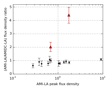
Figure 1: Flux density ratios for compact sources detected in both the AMI_AC-LA survey data and new AMI_DC-LA data. Error bars include local thermal noise estimates as well as a 5% calibration error. Only two sources have varied significantly; these are plotted in red and with triangle markers.

The survey map and inner 19 pointings of the AMI_DC map have similar noise levels of $\approx\,30$ – $40\,\upmu$Jy beam^-1 so we expect the same sources to be detected in this region; in fact five common sources are detected in both. Three sources are detected in the AMI_DC map and not in the AMI_AC map. One of these (AMILA J030032+261849) is next to a brighter source and is not detected due to a combination of the poorer dynamic range in the AMI_AC map and a slightly reduced flux density; we made a manual fit to the nearby sources using jmfit and obtained a flux density of $200\pm 60\upmu$Jy beam^-1, consistent with the AMI_DC flux within the noise levels. The second and third (AMILA J025955+260842 and AMILA J025936+261343) are just visible at $\approx\,3.7\sigma$ and 3.0$\sigma$ respectively in the AMI_AC map and also have consistent flux densities given the noise levels. One source (AMILA J030010+261202) is detected in the AMI_AC map and not in the AMI_DC map; although it should have been detected at 6$\sigma$, there is no trace of it in the map and is probably a variable source caught at higher flux density during the previous observations. The situation is similar in the outer region of the AMI_DC map, where all sources expected to be detected based on the higher noise level of $\approx$ 100 $\upmu$Jy beam^-1 are detected; sources at just under the detection limit are visible in the AMI_DC map.

We therefore have confidence that the overall source environment has not changed significantly between the two sets of observations, and combine both sets of data to reduce the noise level and detect as many sources as possible, while suppressing artefacts in the AMI_AC data. We average in the map plane since the survey and follow-up pointing centres do not coincide, using the noise maps generated by source_find as weights for the average. We do not attempt any correction for the small frequency shift since we will allow for small changes in the source flux density due to calibration offsets and/or variability when modelling the sources. The combined LA map with the positions of the source detections is shown in Fig. 2.

AMI-LA

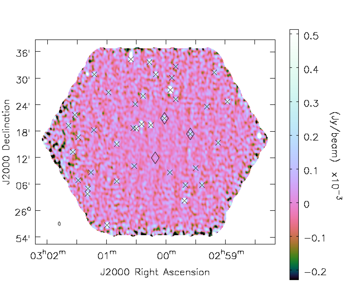
Figure 2: LA map of the compact source environment, made from the combined AMI_AC-LA and AMI_DC-LA datasets. Crosses mark the positions of the detected sources and diamonds mark the positions of the variable sources discussed in Section 4.1. The sources visible at the edges of the map but not marked with crosses are not detected due to failure of the local noise estimation so close to the map edge; they are far enough away from the map centre that failure to subtract them will not affect the SA observations of the target.

4.2 SA data comparison

We first make a qualitative comparison of the AMI_AC-SA and AMI_DC-SA maps. In both cases, clean was run blindly, with no boxes set to influence the choice of clean components, to a threshold of 3 $\times$ the noise on the dirty map. Natural weighting was used. The two maps are shown in Fig. 3. The maps both show a decrement at the centre, with an extension to the south-east; however, the central decrement is deeper in the AMI_AC map at $\approx$ 500 $\upmu$Jy beam^-1 ($\approx\,7.5\sigma$) compared to $\approx$ 300 $\upmu$Jy beam^-1 ($\approx\,6\sigma$) in the AMI_DC map. While the brightness of extended emission in an interferometric map depends on the inclusion and relative weighting of the short baselines present, both datasets have very similar $uv$-plane coverage (and the same physical baselines) so this should not cause the difference. The other noticeable difference between the two maps is the reduced flux density of the compact source to the north of the decrement; this is the variable source AMILA J030001+262059 identified in Section 4.1.

AMI_AC-SA AMI_DC-SA

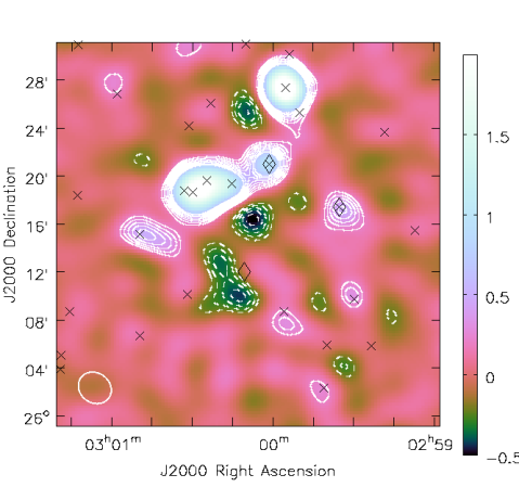
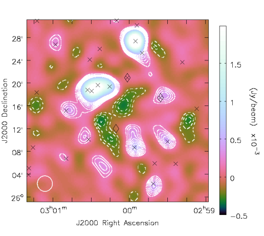
Figure 3: AMI_AC-SA (left) and AMI_DC-SA (right) maps of AMI-CL J0300+2613. The colour-scale is the same in both maps and is truncated to show low-surface-brightness features. White contours (dashed for negative) are overlaid at $\pm 3,4,5,...10\sigma$, where $\sigma$ is the thermal noise measured on the respective maps as given in Table 1. The white ellipse in the left-hand corner of each map shows the synthesised beam, and the crosses and diamonds show the LA source positions as in Fig. 2.

4.3 Cluster analysis

We analysed both datasets using the cluster analysis software package McAdam (Feroz et al., 2009); this fits simultaneously for cluster and compact source parameters while taking into account instrumental noise, primary CMB anisotropies, and confusion from radio sources below the LA detection threshold, in a Bayesian manner using the nested sampling algorithm MultiNest (Feroz, Hobson & Bridges, 2009). For the cluster model, we used a Navarro-Frenk-White (NFW; Navarro, Frenk & White 1997) dark matter profile in hydrostatic equilibrium with a gas pressure distribution described by a generalised NFW (GNFW; Nagai, Kravtsov & Vikhlinin 2007) profile with the shape parameters given in Arnaud et al. (2010); for more details of the model see Olamaie, Hobson & Grainge (2012). We refer to this as the DM-GNFW model. We imposed a joint mass-redshift prior based on the cluster number counts of Tinker et al. (2008) and fixed the gas mass fraction at $r_{200}$ to 0.13 (Komatsu et al., 2011). We set a fairly tight prior on the position of the cluster (a Gaussian with $\sigma=1$ arcmin from the peak of the central decrement visible on the map), to concentrate the analysis on the central decrement.

Each radio source has its position fixed to that determined by the LA. Sources with flux density $>4\sigma$, where $\sigma$ is the noise value on the respective SA map, have their flux density $S$ and spectral index fitted, where the prior on the flux density is Gaussian with a 20% width to account for inter-array calibration uncertainty and possible variability, and the prior on the spectral index is based on the 9C 15 – 22 GHz spectral index distribution (Waldram et al., 2007). Sources with flux density $<4\sigma$ have their flux densities fixed to the LA values, and spectral indices fixed to values determined from Whittam et al. (2013) to be the median of the spectral index distribution at the appropriate flux density. The flux-density priors for the three variable sources (if fitted) are centred at the appropriate value for the epoch and have a wider 40% width since the SA and LA data were not necessarily taken at exactly the same time; all others are as determined from the combined LA map. The parameters and priors on each are summarised in Table 3.

Table 3: Summary of priors used in the Bayesian cluster analysis. The top group of parameters relates to the cluster model while the bottom relates to the radio point sources. ‘NV’ and ‘V’ refer to non-variable and variable point sources, respectively.

Parameter	Prior type	Limits
$x_{0}$, $y_{0}$	$\mathcal{N}(\upmu=\mathrm{map\>peak},$
	$\sigma=1$ arcmin)
$z$	Tinker($z$,$M_{200}$)	[0.2, 2]
$M_{200}$	Tinker($z$,$M_{200}$)	[1, 60] $\times 10^{14}M_{\odot}$
$f_{\mathrm{gas},200}$	$\delta(0.13)$
$x_{s,i}$, $y_{s,i}$	$\delta(\mathrm{LA})$
$S_{i}$ ($S_{i}>4\sigma_{\mathrm{SA}}$, NV)	$\mathcal{N}(\upmu=S_{i,\mathrm{LA}},$
	$\sigma=0.2\times S_{i,\mathrm{LA}})$	[0, $\inf$)
$S_{i}$ ($S_{i}>4\sigma_{\mathrm{SA}}$, V)	$\mathcal{N}(\upmu=S_{i,\mathrm{LA}},$
	$\sigma=0.4\times S_{i,\mathrm{LA}})$	[0, $\inf$)
$\alpha_{i}$ ($S_{i}>4\sigma_{\mathrm{SA}}$)	9C
$S_{i}$ ($S_{i}<4\sigma_{\mathrm{SA}}$)	$\delta(S_{i,\mathrm{LA}})$
$\alpha_{i}$ ($S_{i}<4\sigma_{\mathrm{SA}}$)	$\delta(\alpha(S_{i,\mathrm{LA}}))$

For each dataset, we ran our Bayesian analysis software with a model consisting of cluster and point sources (the ‘cluster’ run), and with point sources only (the ‘null’ run). The ratio between the Bayesian evidences for these two runs can be used for model selection, i.e. to quantify whether the data are more consistent with or without a cluster being present. The AMI_AC data had an evidence ratio of e^9.9, showing significant evidence for a cluster, while the AMI_DC data had an evidence ratio of e^1.4, showing only marginal evidence for the presence of a cluster. Along with the difference in evidence ratios, it can also be seen that the mass posteriors are discrepant; the AMI_AC posterior puts a definite constraint on the mass at $M_{T,200}=(4.54\pm 0.83)\times 10^{14}M_{\odot}$ while the AMI_DC posterior can only provide an upper limit, $M_{T,200}<1.79\times 10^{14}M_{\odot}$; the marginalised mass posteriors are shown, together with the prior, in Fig. 4. Such a different result, for qualitatively similar maps, can be understood if the shape of the decrement in the AMI_DC data in $uv$-space does not agree well with the model. In this case the evidence ratio is decreased, and the posterior on mass becomes dominated by the prior (which strongly prefers low mass) rather than the likelihood, so a much lower mass is preferred even though the decrement in the AMI_DC map is comparable to the decrement in the AMI_AC map.

We next test the robustness of this result by making various changes to the cluster priors and model, including: allowing the cluster to have an ellipsoidal geometry on the plane of the sky; setting a wider positional prior so that the extended ‘tail’ of the decrement to the South is also found by the sampler; increasing the lower limit of the mass prior and using a Jenkins et al. (2001) mass prior so that lower masses are not so strongly preferred by the prior; and changing the model to a purely phenomenological description of the SZ decrement (see AMI Consortium: Shimwell et al. 2012 for details of this model and the parameter priors). Each case is consistent in the general result that the evidence for the presence of a cluster in the AMI_DC data is reduced compared to the AMI_AC data. The DM-GNFW models always indicate a reduced mass, and the phenomenological models always indicate a much more extended decrement (so that more cluster signal is resolved out) and a less negative temperature. The phenomenological models give more significant evidence for the presence of a decrement in the AMI_DC data (but always much lower evidence values than when used with the AMI_AC data).

For the AMI_DC data, since there are significant positive residuals present at the location of some sources on the source-subtracted map (see Fig. 5), we also investigated widening the flux density priors and allowing the positions of some sources to shift slightly, to remove as much positive emission as possible; again, the general result is unchanged.

DM-GNFW model Isothermal $\beta$ model

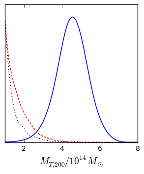
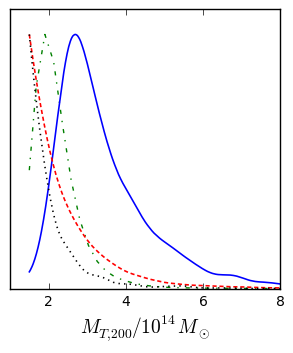
Figure 4: Left: marginalised 1-D mass posteriors as derived from AMI_AC data (blue solid line), AMI_DC data (red dashed line), and the prior distribution (black dotted line), using the DM-GNFW model. Right: mass posteriors and prior as derived using the $\beta$-model, with the addition of the CARMA posterior (green dot-dashed line). Note that the $x$-axis scales are the same for ease of comparison, but the prior lower limit for the $\beta$-model analysis was set to $1.5\times 10^{14}M_{\odot}$.

Since the CARMA analysis was performed using an isothermal $\beta$ model for the cluster gas distribution with priors as listed in AMI Consortium: Shimwell et al. (2012), we also ran the AMI_AC and AMI_DC analysis using the same model and priors for a fair comparison. The resulting mass posteriors, along with those for the CARMA data, are also plotted in Fig. 4, and it can be seen that the AMI_DC posteriors are in much better agreement with the CARMA posteriors than the AMI_AC posteriors.

In Fig. 5 we show the point-source-subtracted AMI_AC and AMI_DC maps, using the source parameters as fitted simultaneously with the cluster parameters (using the DM-GNFW model and the 1 arcmin prior on cluster position). There are significant positive residuals in both maps, indicating the presence of positive extended emission which was not detected on the LA map. This could be a radio relic, which is a region of synchrotron emission caused by acceleration of relativistic electrons by shocks caused by cluster mergers; these are steep spectrum sources but have been detected at 15 GHz (e.g. Stroe et al. 2014; Stroe et al. 2016), or indeed steep-spectrum synchrotron emission resulting from radio-jet activity. We have checked the GaLactic and Extragalactic All-sky MWA (GLEAM) survey (Hurley-Walker et al., 2017), at $\approx$ 200 MHz and with good sensitivity to extended structures, and find no trace of the extended emission (see Fig. 6). Stroe et al. (2016) fitted broken power-law spectra to the integrated flux densities of the two relics that have been detected at 15 GHz, the ‘Sausage’ and ‘Toothbrush’ relics. Using these fits, the relic should be either 450$\times$ or 240$\times$ brighter at 200 MHz than at 15 GHz, respectively. The synthesised beam on the GLEAM map is the same size as the AMI_DC-SA beam to within 4%, and we measure the noise level to be 18.5 mJy beam^-1 using the imean task in aips. The surface brightness of the positive emission ranges from $\approx$ 300 – 650 $\upmu$Jy beam^-1 on the AMI_DC-SA primary-beam-corrected map in the case that we widen the source priors to subtract as much positive emission as possible, so even in the ‘Toothbrush’ case the faintest emission should be visible at $\approx$ 4$\sigma$ on the GLEAM map. We therefore conclude that the positive emission is unlikely to be a radio relic or other form of synchrotron emission.

AMI_AC-SA AMI_DC-SA

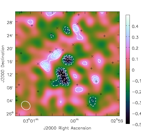
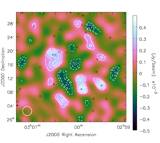
Figure 5: AMI_AC-SA (left) and AMI_DC-SA (right) compact-source-subtracted maps of AMI-CL J0300+2613. The colour-scale is the same in both maps and is not truncated. Contours are as in Fig. 3. The ‘$\times$’ markers show the positions of sources for which the flux density and alpha were modelled simultaneously with the cluster parameters, while the ‘$+$’ markers show the positions of less significant sources which were subtracted using the LA source parameter estimates. The small box shows the McAdam estimate of the cluster centre. The white ellipse in the bottom left-hand corner shows the synthesised beam.

GLEAM 200 MHz

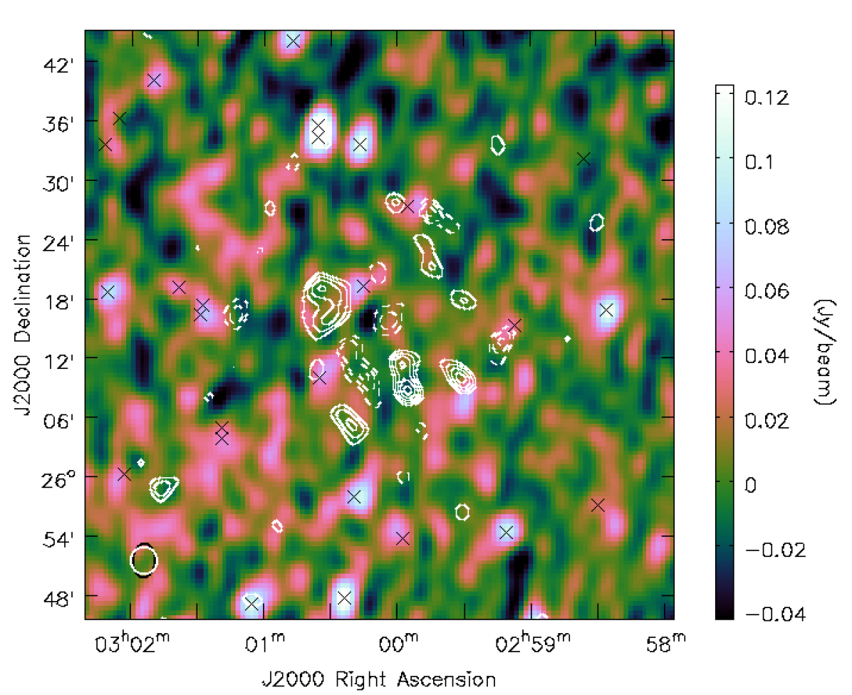
Figure 6: The GLEAM 200 MHz map (colour-scale), overlaid with the AMI_DC-SA source-subtracted contours (in white). The crosses show the positions of low-frequency compact sources from the TIFR GMRT Sky Survey Alternative Data Release (TGSS ADR1; Intema et al. 2017 catalogue. The colour-scale is truncated to show any low-surface-brightness extended features; contours are as in Fig. 3. The white and black ellipses superposed in the bottom left-hand corner show the AMI_DC-SA and GLEAM synthesised beams, respectively.

Given the reduced evidence for the presence of a cluster, we search for alternative explanations for the emission in datasets available at other wavebands.

4.4 Dust emission

Another source of extended positive emission at 15 GHz is dust, either the tail of the greybody distribution or dust-correlated anomalous microwave emission (AME; first detected by Leitch et al. 1997). We therefore compare the source-subtracted SA maps to the Planck High Frequency Instrument (HFI) maps (Planck Collaboration et al., 2016b), the Akari WIDE-L (140  $\upmu$m) and WIDE-S (90 $\upmu$m) band maps (Murakami et al. 2007; Doi et al. 2015), and the Wide-field Infrared Survey Explorer (WISE, Wright et al. 2010) 12- and 25-$\upmu$m maps and find a clear correspondence between the AMI extended emission and a ring of emission visible in all the infrared/sub-mm maps mentioned, even though the AMI survey field was chosen to be well outside the Galactic plane at $\ell=155.8^{\circ},b=-28.3^{\circ}$. Fig. 7 shows the AMI_DC-SA source-subtracted contours overlaid on the Akari WIDE-L-band map. There is a clear correspondence between bright knots of emission in the filamentary dust structure and the AMI positive emission; the negative feature sits in the centre of the ring where there is less dust emission.

Akari WIDE-L (140 $\upmu$m)

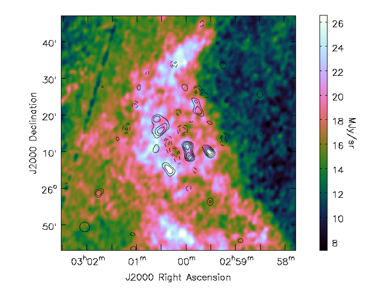
Figure 7: The Akari WIDE-L ($140\,\upmu$m) map (colour-scale), overlaid with the AMI_DC-SA source-subtracted contours (in black). The colour-scale is truncated to show low-surface-brightness extended features; contours are as in Fig. 3. The black ellipse in the bottom left-hand corner shows the AMI_DC-SA synthesised beam.

Comparisons with interferometric observations of resolved sources must take into account the spatial filtering applied by the interferometer. This can be achieved by simulating interferometric observations of a sky model containing all relevant angular scales; i.e. at significantly higher angular resolution than the sky model and containing the large angular scales partially resolved out by the interferometer. To further test the apparent AMI-dust correspondence, we simulated AMI observations of the Akari WIDE-L- and WIDE-S-band and the Meisner & Finkbeiner (2014) source-subtracted WISE 12 $\upmu$m maps, which have angular resolutions 88, 78 and 15 arcsec respectively. The Planck HFI maps are too low-resolution for this procedure and the WISE 25-$\upmu$m maps are complicated by the presence of point sources. We used the same $uv$-plane sampling as in the real AMI_DC-SA observations and did not add any noise. Since the $uv$-coordinates correspond to baseline length measured in $\lambda$, meaning that slightly different angular scales are sampled at different frequencies, we simulated eight frequency channels covering the AMI band with the same sky brightness (i.e. no spectral index correction was applied to the infrared maps). Maps of these simulations, imaged in the same way as the AMI_DC-SA data, are shown in Fig. 8. We tested the apparent correspondence in both the $uv$- and map-planes: for each dust simulation, we calculated Pearson correlation coefficients between the simulated and the real (point-source-subtracted) AMI_DC-SA visibilities, and also between the simulated and real map pixels. The correlation coefficients are listed in Table 4. We note that the $uv$-plane-based $r$-values are quite low due to the low signal-to-noise on each visibility measurement, but due to the large number of measurements they are still significant as shown by the very low $p$-values (which indicate the probability of an uncorrelated system producing datasets with $r$-values at least as extreme as the calculated $r$-value). We also note the natural tendency for the $r$-values to decline with frequency due to more of the extended emission being resolved out; this is also seen, for example, if we calculate $r$-values between the two Akari simulations. The ‘Channel 1’ correlation coefficients tend to be lower, probably due to higher noise in this frequency bin.

Akari WIDE-L (140 $\upmu$m) Akari WIDE-S (90 $\upmu$m)      WISE 12 $\upmu$m

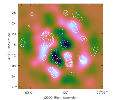
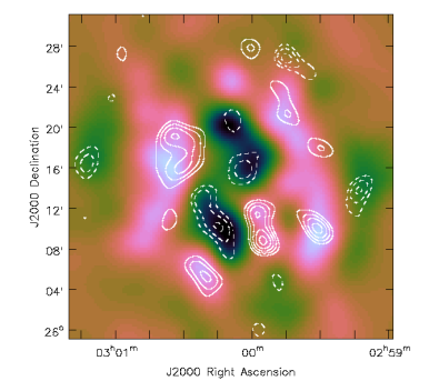
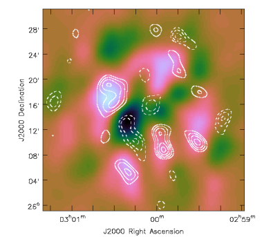
Figure 8: Simulated AMI_DC-SA observations of the Akari WIDE-L (left) and WIDE-S (centre) band and WISE 12 $\upmu$m (right) maps, with no added noise. Colour scales are arbitrary; the zero level is orange. The white contours show the AMI_DC-SA compact-source-subtracted residuals as in Fig. 3.

Table 4: Pearson $r$-values and $p$-values (as calculated by the scipy.stats.pearsonr module) for AMI_DC-SA and simulated Akari and WISE observations, both in the map- and $uv$-plane. For the $uv$-plane based correlations we quote values for the eight simulated channels.

Type	AMI	Aux	$r$	$p$
	channel	data
Map	all	WIDE-L	0.2748	0.00
Map	all	WIDE-S	0.2669	0.00
Map	all	WISE-12	0.2170	0.00
$uv$	1	WIDE-L	0.0078	$4.10\times 10^{-04}$
$uv$	2	WIDE-L	0.0138	$2.86\times 10^{-10}$
$uv$	3	WIDE-L	0.0145	$3.30\times 10^{-11}$
$uv$	4	WIDE-L	0.0112	$3.37\times 10^{-07}$
$uv$	5	WIDE-L	0.0101	$2.57\times 10^{-06}$
$uv$	6	WIDE-L	0.0088	$4.29\times 10^{-05}$
$uv$	7	WIDE-L	0.0069	$1.28\times 10^{-03}$
$uv$	8	WIDE-L	0.0087	$4.91\times 10^{-05}$
$uv$	1	WIDE-S	0.0080	$3.19\times 10^{-04}$
$uv$	2	WIDE-S	0.0148	$1.57\times 10^{-11}$
$uv$	3	WIDE-S	0.0139	$1.95\times 10^{-10}$
$uv$	4	WIDE-S	0.0116	$1.04\times 10^{-07}$
$uv$	5	WIDE-S	0.0093	$1.44\times 10^{-05}$
$uv$	6	WIDE-S	0.0072	$8.20\times 10^{-04}$
$uv$	7	WIDE-S	0.0051	$1.78\times 10^{-02}$
$uv$	8	WIDE-S	0.0099	$3.82\times 10^{-06}$
$uv$	1	WISE-12	0.0080	$3.00\times 10^{-04}$
$uv$	2	WISE-12	0.0116	$1.09\times 10^{-07}$
$uv$	3	WISE-12	0.0154	$1.90\times 10^{-12}$
$uv$	4	WISE-12	0.0086	$7.91\times 10^{-05}$
$uv$	5	WISE-12	0.0078	$2.82\times 10^{-04}$
$uv$	6	WISE-12	0.0058	$6.71\times 10^{-03}$
$uv$	7	WISE-12	0.0055	$1.05\times 10^{-02}$
$uv$	8	WISE-12	0.0071	$1.04\times 10^{-03}$

4.5 Ring/decrement degeneracy

To understand how a ring of positive emission can appear as a decrement, both visually in the map plane and in the $uv$-plane McAdam analysis (which only accounts for negative cluster emission and point sources), we performed some simple simulations. We simulated a ring of emission of 6-arcmin thickness and a 6-arcmin inner radius, approximately mimicking the infrared emission, and a negative Gaussian with a 6-arcmin FWHM, approximating a cluster decrement. In Fig. 9 we show the visibilities corresponding to these simulations (i.e. the simulation multiplied by the AMI-SA primary beam and Fourier transformed). The ‘ring’ visibilities have a negative real component on the same scale as the ‘cluster’ decrement, and given the lack of baselines at $<200\lambda$ it would clearly be very difficult for the $uv$-plane analysis to distinguish between these two morphologies once noise is added, even with these very simple models. Examining the more complicated Fourier transform of the Akari maps, we see similar features. This explains why the McAdam analysis marginally prefers the cluster model, even for the AMI_DC-SA data.

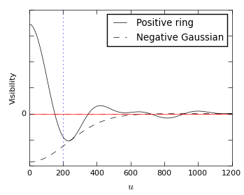
Figure 9: Real (black) and imaginary (red; insignificant due to symmetry) visibilities corresponding to a ring of positive emission and a negative Gaussian (see text for details), as a function of distance from the centre of the $uv$-plane, $u$, which corresponds to projected baseline length in units of $\lambda$. The dotted blue vertical line shows the minimum projected SA baseline length. The $y$-scale is arbitrary and the simulations have been normalised to have the same amplitude at $u=250\lambda$.

In the map plane, the degeneracy can be understood by considering the simulated dirty maps, which are the sky surface brightness convolved with the dirty beam, the Fourier transform of the $uv$-coverage. Fig. 10 shows the dirty beam and $uv$-coverage for the AMI_DC-SA observations, and Fig. 11 shows the dirty maps for the two simulations. In this case the simulated ring has inner and outer radii of 4 and 8 arcmin respectively, to better illustrate the problem. The dirty beam has negative sidelobes of $\approx$ 25% amplitude. In the case of the ring, the negative sidelobes add up in the centre, producing a decrement of similar surface brightness to the positive ring. The positive ring has brighter spots approximately aligned to the east–west axis; this is due to the ellipsoidal shape of the $uv$-coverage. In the case of the decrement, the dirty map has positive bright spots in a similar place, which are produced by the negative beam sidelobes becoming positive when convolved with the decrement. As in the $uv$-plane, it is very difficult to distinguish between these two morphologies without any additional information.

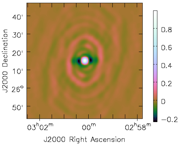
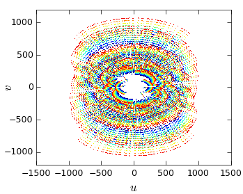
Figure 10: Dirty beam (left) and $uv$-coverage (right; i.e. projected baseline length in units of $\lambda$) for the AMI_DC-SA data. Colours in the $uv$-coverage plot represent the 8 frequency bins; only every 120th point has been plotted for clarity.

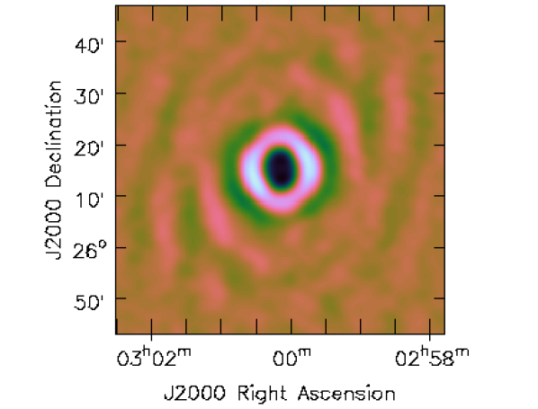
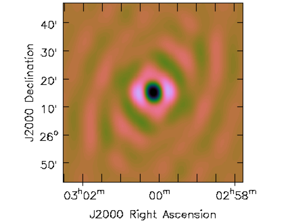
Figure 11: Simulated AMI_DC-SA dirty maps of a 4 arcmin wide ring with a 4 arcmin inner radius (left) and a negative Gaussian with a 6 arcmin FWHM (right). Colour scales are arbitrary; the zero level is orange.

The higher significance of the decrement in the AMI_AC-SA map can also be explained as follows. The analogue correlator had an imperfect point-source response which produced positive and negative ringing around sources. If negative residuals from the positive emission in the ring happened to be at the right distance to add coherently in the same way as the dirty-beam sidelobes, this would produce an enhanced decrement, both in the map and the $uv$-plane analysis. This also explains why the decrement remains significant in the AMI_AC-SA map after source subtraction – idealised point-source subtraction does not remove the contribution from the artefacts. From here on, we will concentrate on the AMI_DC-SA data.

4.6 Re-imaging the AMI_DC-SA data

Since we now believe the decrement to be a misinterpretation of the interferometric measurement of the positive ring, we re-cleaned the AMI_DC-SA data interactively, placing clean boxes around the areas of positive emission rather than allowing clean components to be blindly placed in the most positive/negative regions. This decreased the significance of both the central ‘decrement’ and the more extended negative features to the south to $3\sigma$ or less, while increasing the significance of the positive features.

4.7 Free–free analysis

Extended, optically thin free–free emission could also account for the positive emission seen at 15 GHz. However, this is not a known star-forming region and checking the Tóth et al. (2014) and Marton et al. (2016) young-stellar-object (YSO) catalogues we find only one YSO candidate (AllWISE J030209.94+260045.9) nearby, well outside the AMI primary beam. We therefore consider free–free unlikely to be the mechanism for the emission, but none-the-less check for visible emission at 5 GHz in the GB6 survey map (Condon et al., 1994), which at resolution 3.5 arcmin and containing angular scales up to $\approx$ 20 arcmin has the correct spatial information. We see no trace of the emission on the GB6 map; see Fig. 12.

GB6 5 GHz

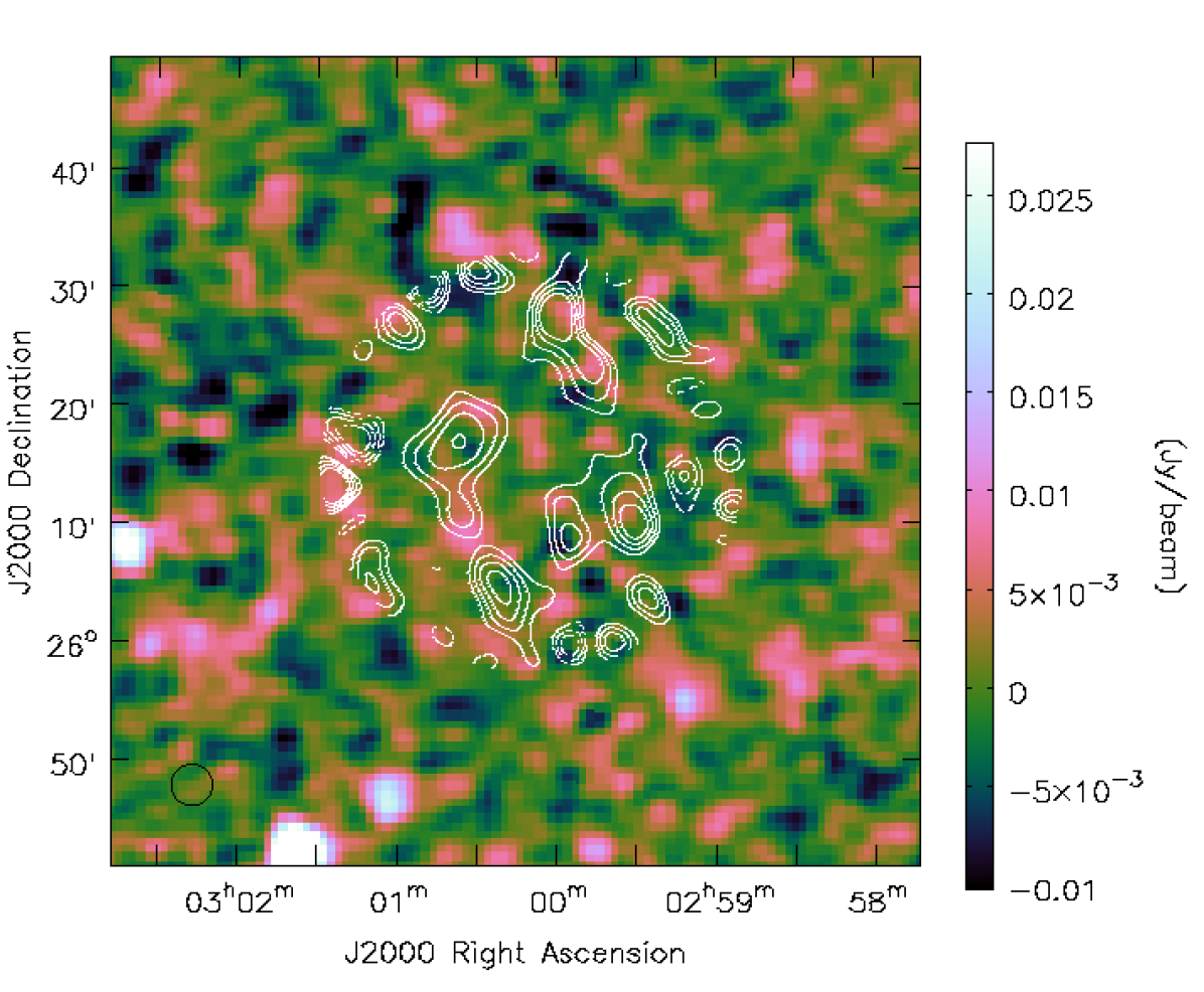
Figure 12: The GB6 (5 GHz) map (colour-scale), overlaid with the AMI_DC-SA source-subtracted contours (in white), convolved to the GB6 resolution and extrapolated to 5 GHz using $\alpha=0.1$. The colour-scale is truncated to show any low-surface-brightness extended features; contours are at ($\pm$4, 6, 8, 10) $\times$ 0.1 mJy beam^-1. Features at the edge of the AMI_DC primary beam are due to increased noise. The black circle in the bottom left-hand corner shows the GB6 beam.

We convolve the AMI_DC-SA map down to the GB6 resolution and extrapolate to 5 GHz using the canonical optically-thin power-law index of $\alpha=0.1$. The maximum surface brightness on the extrapolated map is $\approx$ 1.0 mJy beam^-1, while the GB6 map has a relatively high noise level of $\approx$ 3 mJy beam^-1. However, this is an upper limit given that the emission is clearly very resolved. Using the simulated AMI_DC observation of the Akari Wide-S map (see Section 4.4), which has the best correlation with the AMI_DC data, we estimate a scaling factor of $1.7\times 10^{-4}$ to make the simulated Akari visibilities consistent with the AMI_DC visibilities. An estimate of the emission at 15 GHz with all spatial scales present can therefore be made by scaling the Akari map by this factor. We then fit a twisted plane background to a polygon with edges surrounding the ring of emission, excluding the northern extension (see, e.g. Green 2007). We subtract this background to remove the largest scales which are not visible to GB6; convolve to the GB6 resolution and extrapolate to 5 GHz using $\alpha=0.1$. In this case the surface brightness is $\approx\,7$ – 10 mJy beam^-1 and should be detectable by GB6. While the correlation between the emission seen by AMI and Akari is not perfect and so we cannot use this argument to conclusively rule out free–free as the origin of this emission, it seems unlikely.

4.8 Greybody tail or AME?

The Planck 2015 data release (Planck Collaboration et al., 2016a) included component-separated maps and fitted dust model parameter maps from several different methods. We used the generalized needlet, internal linear combination (GNILC) (Planck Collaboration et al., 2016d) dust parameter estimate maps to extrapolate the modified black-body emission fit to the AMI band and find that the expected thermal emission is at least $\approx\,20\,\times$ fainter than the observed AMI flux density, even before any spatial filtering of the extended emission is applied. We therefore consider it very unlikely that the AMI emission is simply thermal emission and conclude that it is most likely to be AME. We note that the Planck component-separated AME map (Planck Collaboration et al., 2016c) shows some structure in this region, which is $\approx\,10^{\circ}$ from the well-known AME region in Perseus (e.g. Watson et al. 2005; Tibbs et al. 2013), but the sensitivity and angular resolution are both too low for a detection. No emission is visible above the noise levels in the Planck Low Frequency Instrument (LFI) maps, so we cannot construct a spectral energy distribution to check for the characteristic peak which would confirm the AME nature of the emission.

5 Discussion

A strong contender for the origin of AME is electric dipole emission from rapidly rotating very small dust grains, with polycyclic aromatic hydrocarbons (PAHs) considered to be natural carriers of the emission due to their abundance and appropriate size (Draine & Lazarian 1998a; Draine & Lazarian 1998b). However, a definitive observational link between PAH abundance and AME has not been shown. Some studies have shown greater correlations between 12-$\upmu$m emission, tracing the PAH abundance, than with longer wavelengths which trace the larger grains (e.g. Casassus et al. 2006; Ysard, Miville-Deschênes & Verstraete 2010) but the majority show no significant difference (e.g. Tibbs et al. 2011; Planck Collaboration et al. 2014; Hensley, Draine & Meisner 2016). These AMI observations are consistent with the latter conclusion, since the 12-$\upmu$m simulation correlates slightly worse than the longer-wavelength simulations; however, none of the simulations is completely consistent with the AMI map, with parts of the emission (e.g. the eastern side of the ring in the Akari maps, and the northern side of the ring in the WISE map) visible in the infra-red yet not visible by AMI.

This represents the only blind detection of AME on arcminute scales. All previous blind detections (e.g. Leitch et al. 1997; Watson et al. 2005; Ysard, Miville-Deschênes & Verstraete 2010; Planck Collaboration et al. 2016c) have been at scales $>10$ arcmin; higher-resolution detections have all been targeted observations of specific objects. The AMI galaxy cluster survey can also be seen as a very deep survey for AME; we plan to reanalyse the rest of this survey field to search for additional positive extended structures and reobserve them with AMI_DC. For example, it is clear that the bright northern extension of the ring is also seen in the AMI survey data (see Fig. 13). More information is required to probe the nature of the AME in this field, including higher-frequency radio data to investigate the AME spectrum (we note that the CARMA observation did not contain enough short baselines to be useful in this regard), and high-resolution infra-red data in more bands to properly investigate the dust properties. With more information, this survey could provide important clues as to the nature of AME given that the detection presented here does not appear to be associated with the usual AME-producers such as star-forming regions and dark clouds.

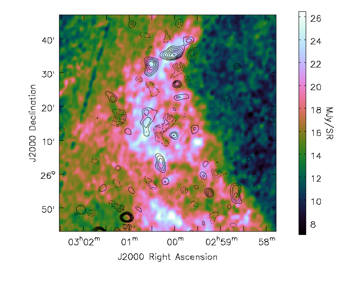
Figure 13: The Akari Wide-L map of the region (colour-scale), overlaid with AMI-SA survey source-subtracted significance contours (in black). Contours are at ($\pm$3, 4, 5, …, 10) $\times$ the local noise level on the map. The black ellipse in the bottom left-hand corner shows the AMI-SA beam.

6 Conclusions

We have reobserved AMI-CL J0300+2613, reported in AMI Consortium: Shimwell et al. (2012) to be a galaxy cluster detected via its SZ effect, with AMI equipped with a new digital correlator. We find that:

1. The SZ-decrement evidence for the presence of a cluster is much reduced in the AMI_DC data compared to the AMI_AC data, although the decrement is still visible in the map at lower significance.

2. By comparison with high-resolution sub-mm and infra-red maps that were not available at the time of the initial detection, we find that the apparent decrement is actually a misinterpretation of the interferometric measurement of a ring of dust-correlated emission.

3. Although we cannot entirely rule out free–free as the origin of the 15-GHz emission, we suggest that its origin is most likely to be Galactic AME, making it the first blind detection of AME on arcminute scales

4. Assuming the emission is AME, our analysis agrees with recent results that the AME does not necessarily correlate better with the 12-$\upmu$m emission which traces the PAH abundance.

5. We plan to reobserve other parts of the AMI blind cluster survey field to search for more AME from the structure visible in the infra-red maps.

References

- AMI Consortium: Davies et al. (2011) AMI Consortium: Davies, M. L., et al., 2011, MNRAS, 415, 2708
- AMI Consortium: Franzen et al. (2011) AMI Consortium: Franzen, T. M. O., et al., 2011, MNRAS, 415, 2699
- AMI Consortium: Shimwell et al. (2012) AMI Consortium: Shimwell T. W., et al., 2012, MNRAS, 423, 1463
- AMI Consortium: Shimwell et al. (2013) AMI Consortium: Shimwell T. W., et al., 2013, MNRAS, 433, 2036
- Arnaud et al. (2010) Arnaud M., Pratt G. W., Piffaretti R., Böhringer H., Croston J. H., Pointecouteau E., 2010, A&A, 517, A92
- Casassus et al. (2006) Casassus S., Cabrera G. F., Förster F., Pearson T. J., Readhead A. C. S., Dickinson C., 2006, ApJ, 639, 951
- Condon et al. (1994) Condon J. J., Broderick J. J., Seielstad G. A., Douglas K., Gregory P. C., 1994, AJ, 107, 1829
- Doi et al. (2015) Doi Y., et al., 2015, PASJ, 67, 50
- Draine & Lazarian (1998a) Draine B. T., Lazarian A., 1998a, ApJ, 494, L19
- Draine & Lazarian (1998b) Draine B. T., Lazarian A., 1998b, ApJ, 508, 157
- Feroz, Hobson & Bridges (2009) Feroz F., Hobson M. P., Bridges M., 2009, MNRAS, 398, 1601
- Feroz et al. (2009) Feroz F., Hobson M. P., Zwart J. T. L., Saunders R. D. E., Grainge K. J. B., 2009, MNRAS, 398, 2049
- Green (2007) Green D. A., 2007, Bulletin of the Astronomical Society of India, 35, 77
- Green (2011) Green D. A., 2011, Bulletin of the Astronomical Society of India, 39, 289
- Hensley, Draine & Meisner (2016) Hensley B. S., Draine B. T., Meisner A. M., 2016, ApJ, 827, 45
- Hickish et al. (2017) Hickish J., et al., 2017, arXiv:1707.04237
- Hurley-Walker et al. (2017) Hurley-Walker N., et al., 2017, MNRAS, 464, 1146
- Intema et al. (2017) Intema H. T., Jagannathan P., Mooley K. P., Frail D. A., 2017, A&A, 598, A78
- Jenkins et al. (2001) Jenkins A., Frenk C. S., White S. D. M., Colberg J. M., Cole S., Evrard A. E., Couchman H. M. P., Yoshida N., 2001, MNRAS, 321, 372
- Komatsu et al. (2011) Komatsu E., et al., 2011, ApJS, 192, 18
- Leitch et al. (1997) Leitch E. M., Readhead A. C. S., Pearson T. J., Myers S. T., 1997, ApJ, 486, L23
- Marton et al. (2016) Marton G., Tóth L. V., Paladini R., Kun M., Zahorecz S., McGehee P., Kiss C., 2016, MNRAS, 458, 3479
- Meisner & Finkbeiner (2014) Meisner A. M., Finkbeiner D. P., 2014, ApJ, 781, 5
- Muchovej et al. (2007) Muchovej S., et al., 2007, ApJ, 663, 708
- Murakami et al. (2007) Murakami H., et al., 2007, PASJ, 59, S369
- Nagai, Kravtsov & Vikhlinin (2007) Nagai D., Kravtsov A. V., Vikhlinin A., 2007, ApJ, 668, 1
- Navarro, Frenk & White (1997) Navarro J. F., Frenk C. S., White S. D. M., 1997, ApJ, 490, 493
- Olamaie, Hobson & Grainge (2012) Olamaie M., Hobson M. P., Grainge K. J. B., 2012, MNRAS, 423, 1534
- Perley & Butler (2013a) Perley R. A., Butler B. J., 2013a, ApJS, 206, 16
- Perley & Butler (2013b) Perley R. A., Butler B. J., 2013b, ApJS, 204, 19
- Planck Collaboration et al. (2014) Planck Collaboration, et al., 2014, A&A, 565, A103
- Planck Collaboration et al. (2016a) Planck Collaboration, et al., 2016a, A&A, 594, A1
- Planck Collaboration et al. (2016b) Planck Collaboration, et al., 2016b, A&A, 594, A8
- Planck Collaboration et al. (2016c) Planck Collaboration, et al., 2016c, A&A, 594, A10
- Planck Collaboration et al. (2016d) Planck Collaboration, et al., 2016d, A&A, 596, A109
- Stroe et al. (2014) Stroe A., et al., 2014, MNRAS, 441, L41
- Stroe et al. (2016) Stroe A., et al., 2016, MNRAS, 455, 2402
- Sunyaev & Zeldovich (1972) Sunyaev R. A., Zeldovich Y. B., 1972, Comments on Astrophysics and Space Physics, 4, 173
- Tibbs et al. (2011) Tibbs C. T., et al., 2011, MNRAS, 418, 1889
- Tibbs et al. (2013) Tibbs C. T., Scaife A. M. M., Dickinson C., Paladini R., Davies R. D., Davis R. J., Grainge K. J. B., Watson R. A., 2013, ApJ, 768, 98
- Tinker et al. (2008) Tinker J., Kravtsov A. V., Klypin A., Abazajian K., Warren M., Yepes G., Gottlöber S., Holz D. E., 2008, ApJ, 688, 709
- Tóth et al. (2014) Tóth L. V., et al., 2014, PASJ, 66, 17
- Waldram et al. (2007) Waldram E. M., Bolton R. C., Pooley G. G., Riley J. M., 2007, MNRAS, 379, 1442
- Watson et al. (2005) Watson R. A., Rebolo R., Rubiño-Martín J. A., Hildebrandt S., Gutiérrez C. M., Fernández-Cerezo S., Hoyland R. J., Battistelli E. S., 2005, ApJ, 624, L89
- Whittam et al. (2013) Whittam I. H., et al., 2013, MNRAS, 429, 2080
- Wright et al. (2010) Wright E. L., et al., 2010, AJ, 140, 1868
- Ysard, Miville-Deschênes & Verstraete (2010) Ysard N., Miville-Deschênes M. A., Verstraete L., 2010, A&A, 509, L1
- Zwart et al. (2008) Zwart J. T. L. et al., 2008, MNRAS, 391, 1545