Dark matter scenarios with multiple spin-2 fields

Abstract

We study ghost-free multimetric theories for $(N+1)$ tensor fields with a coupling to matter and maximal global symmetry group $S_{N}\times(Z_{2})^{N}$. Their mass spectra contain a massless mode, the graviton, and $N$ massive spin-2 modes. One of the massive modes is distinct by being the heaviest, the remaining $(N-1)$ massive modes are simply identical copies of each other. All relevant physics can therefore be understood from the case $N=2$. Focussing on this case, we compute the full perturbative action up to cubic order and derive several features that hold to all orders in perturbation theory. The lighter massive mode does not couple to matter and neither of the massive modes decay into massless gravitons. We propose the lighter massive particle as a candidate for dark matter and investigate its phenomenology in the parameter region where the matter coupling is dominated by the massless graviton. The relic density of massive spin-2 can originate from a freeze-in mechanism or from gravitational particle production, giving rise to two different dark matter scenarios. The allowed parameter regions are very different from those in scenarios with only one massive spin-2 field and more accessible to experiments.

1 Introduction

Field theories with massive spin-2 degrees of freedoms have developed into a topic of interest in particle physics and cosmology; see Hinterbichler:2011tt ; deRham:2014zqa ; Schmidt-May:2015vnx for recent reviews. Massive spin-2 particles may be viewed as a natural addition to the Standard Model (SM) combined with General Relativity (GR), since the first contains massive and massless particles up to spin-1 and the latter describes a massless spin-2 particle, the graviton. The linear Fierz-Pauli theory for massive spin-2 was already developed in 1939 Fierz:1939ix , but it suffers from a discontinuous zero-mass limit, known as the vDVZ discontinuity vanDam:1970vg ; Zakharov:1970cc . Due to this, the Fierz-Pauli theory is not compatible with basic solar system tests. A possible solution to this problem is the inclusion of nonlinear interactions giving rise to a Vainshtein screening mechanism Vainshtein:1972sx that can cure the discontinuity. Unfortunately, for decades nonlinear interactions for massive spin-2 fields were believed to generally contain a fatal ghost instability Boulware:1973my . This problem was resolved only a few years ago when a set of consistent interactions was identified and proven to avoid the ghost deRham:2010ik ; deRham:2010kj ; Hassan:2011vm ; Hassan:2011hr ; Hassan:2011tf ; Hassan:2011ea ; Hassan:2012qv . The resulting theory contains a massive tensor field $g_{\mu\nu}$ that can couple to SM matter and thereby mediate gravitational interactions. Since the gravitational force is long-ranged, the spin-2 mass is constrained to be extremely small (essentially on the order of the Hubble scale) in this setup.

The ghost-free massive gravity action also contains a second tensor field $f_{\mu\nu}$ which is non-dynamical and merely acts as a fixed reference metric. It has later been realised that, in perturbation theory around any background solution $g_{\mu\nu}$, the reference metric can be traded against certain functions of the curvature of $g_{\mu\nu}$. Hassan:2013pca ; Bernard:2014bfa ; Bernard:2015mkk ; Bernard:2015uic ; Mazuet:2017hey . Completely new possibilities opened when it was shown that the second tensor can be given its own dynamics without reintroducing the ghost Hassan:2011zd ; Hassan:2011ea . This results in a bimetric theory for gravity, describing nonlinear interactions of massless and massive spin-2 fields and their couplings to SM matter Hassan:2012wr .

Due to the presence of the massless mode that can mediate a long-range force, the constraints on the spin-2 mass are now much less severe. In fact, it has been shown that the gravitational interactions in bimetric theory can resemble those of GR to any precision for any value of the mass Baccetti:2012bk ; Hassan:2014vja ; Akrami:2015qga ; Babichev:2016bxi . This is achieved by weakening the coupling of the massive spin-2 field to the matter sector. Interestingly, this does not affect the couplings between massive and massless spin-2 fields and the massive mode continues to gravitate with the same strength as the SM fields.

These insights suggest that a relic density of massive spin-2 particles could act as a dark matter (DM) component in the Universe. The existence of DM has been inferred from various astrophysical and cosmological observations but the particle has never been seen other than through its gravitational interactions. In standard scenarios, a model-dependent production mechanism is responsible for creating the DM relic density in the early Universe. Additional symmetries or the very weak interactions of the DM particle ensure its stability until the present time. So far, all attempts to produce or detect the DM particle have remained unsuccessful (see e.g. Agashe:2014kda ; Ackermann:2015lka ), suggesting that it is very heavy and/or its interactions with baryonic matter are simply too weak.

Pursuing (rather speculative) ideas first mentioned in Maeda:2013bha ; Schmidt-May:2016hsx , a possible scenario for massive spin-2 DM was proposed and thoroughly analysed in Babichev:2016hir ; Babichev:2016bxi (see also Aoki:2016zgp ). It was found that ghost-free bimetric theory provides a natural framework for a DM candidate with spin-2 and a mass of a few TeV. Its observed abundance can be explained by invoking a non-thermal (“freeze-in”) production mechanism and the decay products of the particle could in principle be seen in indirect detection experiments. For a recent review of the “freeze-in” mechanism see Bernal:2017kxu . The authors of Chu:2017msm pointed out that strong spin-2 self-interactions can affect the production mechanism by allowing for a thermalisation of the dark sector, and the DM mass could be as low as 1 MeV. Ideas related to these scenarios and extensions were developed in Marzola:2017lbt ; Aoki:2017ffl ; Aoki:2017cnz . Unfortunately, while providing a theoretically well-motivated model, bimetric theory predicts a DM candidate whose interactions with baryonic matter are too tiny to ever be directly detected. For the same reason, it is impossible to produce the massive spin-2 field in colliders. Unless one is lucky and observes its decay products in indirect detection experiments, there are few possibilities to test the model.

It is an interesting question how the phenomenology of massive spin-2 fields is affected by considering more than one species of them. The corresponding ghost-free multimetric interactions were first considered in the vierbein language in Hinterbichler:2012cn . The vierbeins are subject to certain symmetrisation constraints which ensure the absence of ghost instabilities Deffayet:2012zc ; deRham:2015cha and at the same time allow the interactions to be expressed in terms of metric tensors alone Hinterbichler:2012cn ; Hassan:2012wt . The resulting set of consistent theories contain pairwise bimetric interactions between the tensor fields which are not allowed to form a closed loop Nomura:2012xr . They describe one massless spin-2 interacting with several massive spin-2 fields. Their mass spectra were investigated in Baldacchino:2016jsz ; a first analysis of cosmological solutions for theories with three tensors was performed in Luben:2016lku . For more related work, see Noller:2013yja ; Noller:2015eda ; Scargill:2015wxs .

Bimetric theory can be viewed as the extension of GR by one massive tensor and naïvely one may expect that adding more tensor fields will not lead to new physical effects. The aim of this paper is to demonstrate the opposite and present some of the immediate implications for DM phenomenology.

Summary of results.

• An underlying reason for the occurrence of new structures in multimetric interactions with respect to bimetric theory is the possibility to make them invariant under discrete symmetry groups. We argue that the maximal global symmetry in multimetric theories with $(N+1)$ tensors and a coupling to matter is $S_{N}\times(Z_{2})^{N}$ and we identify the corresponding actions.

• The mass spectrum of models with $S_{N}\times(Z_{2})^{N}$ invariance is used to study features of the perturbative action. Moreover, we explicitly compute all cubic interaction vertices in terms of the mass eigenstates for the case $N=2$ which we refer to as “trimetric theory”.

• We find that trimetric theory with maximal global symmetry is a nontrivial generalisation of the $N=1$ case. Just like bimetric theory, it contains a parameter $\alpha$ which together with the spin-2 mass scale controls the deviations from GR. We focus on the case $\alpha<1$ for which these deviations are small over a large mass range. The heaviest spin-2 field behaves very similarly to the massive mode of bimetric theory; it does not decay into massless gravitons and not into lighter spin-2 fields. Its couplings to SM matter are extremely weak. The lighter massive field, however, possesses new features. In particular, it does not interact with matter at all and it cannot decay into other spin-2 particles either. Hence, it is entirely stable. No new phenomena occur for more than three fields; the additional modes all have equal mass and are simply identical copies of the lighter mode in trimetric theory.

• We propose that the observed DM abundance could be made up from the massive spin-2 particles of maximally symmetric trimetric theory. For $\alpha\lesssim 10^{-12}$, this scenario essentially gives rise to a phenomenology that is indistinguishable from the bimetric one. However, in the parameter region where the heaviest mode is not stable enough to contribute to the DM abundance, indirect detection experiments and stability of DM do not put an upper bound on the parameter $\alpha$. In this case, the lighter spin-2 mode is the only DM candidate, giving rise to an entirely new phenomenology. Its relic density can be produced either through a freeze-in mechanism or via gravitational particle production. In the first scenario, the bounds on the spin-2 mass $m$ are,

  $$1\,\mathrm{TeV}\lesssim m\lesssim 10^{11}\,\mathrm{GeV}\,,$$ (1)

  whereas the second production mechanism requires

  $$m\gtrsim 10^{10}\,\mathrm{GeV}\,.$$ (2)

• In the above parameter region with $\alpha<1$, the massive spin-2 particles unfortunately still remain unobservable, at least through direct detection experiments or production in colliders. However, our results suggest that, in contrast to the bimetric DM scenario, the trimetric model contains a new interesting region in its parameter space, corresponding to $\alpha>1$. Here it may become possible to test the model with astrophysical and cosmological observations or even detect the heaviest spin-2 particle directly.

Organisation of the paper.

The paper is organised as follows. In section 2 we briefly review multimetric interactions before identifying the theories with maximal global symmetries. The mass spectrum of maximally symmetric trimetric theory is reviewed in section 3. Section 4 discusses the perturbative expansion of the trimetric action and the generalisation to multiple fields. The implications on DM phenomenology are studied in section 5. We discuss our results and give an outlook in section 6. Appendix A contains the full expressions for cubic vertices in trimetric theory.

2 Multimetric theory

We begin by defining the structure of multimetric actions and discuss how imposing global symmetries singles out a class of models with a significantly smaller parameter space.

2.1 Multimetric interactions

We consider a set of $(N+1)$ tensor fields $f_{\mu\nu}^{(i)}$, $i=1,\ldots,N+1$ and their ghost-free couplings. The fields can only interact pairwise with each other and the interaction graphs cannot contain closed loops. The pairwise interactions arise through a potential,

$$S_{\mathrm{int}}[f^{(i)},f^{(j)}]=-2m^{2}\int\mathrm{d}^{4}x~{}\sqrt{|g|}\,V(f^{(i)},f^{(j)};\beta^{(ij)}_{n})\,,$$ (3)

whose structure is almost entirely fixed by requiring the absence of ghosts. The parameter $m^{2}$ in front has mass dimension two and the potential can be written in the form,

$$V(g,f;\beta_{n})=\sum_{n=0}^{4}\beta_{n}e_{n}\big{(}\sqrt{g^{-1}f}\,\big{)}\,,$$ (4)

with a set of dimensionless parameters $\beta_{n}$, $n=0,\ldots 4$. The (1,1) tensor $\big{(}\sqrt{g^{-1}f}\,\big{)}^{\mu}_{~{}\nu}$ is a matrix square-root defined via $\big{(}\sqrt{g^{-1}f}\,\big{)}^{2}=g^{-1}f$. The elementary symmetric polynomials $e_{n}(S)$ are scalar functions of the matrix argument $S$ and can be defined recursively through,

$$e_{n}(S)=\frac{(-1)^{n+1}}{n}\sum_{k=0}^{n-1}(-1)^{k}\mathrm{Tr}(S^{n-k})e_{k}(S)\,,\qquad e_{0}(S)=1\,.$$ (5)

We furthermore introduce a coupling to SM matter fields which we collectively denote by $\phi$. This coupling must have the same form as in GR,

$$S_{\mathrm{matter}}[g,\phi]=\int d^{4}x~{}\sqrt{|g|}\,\mathcal{L}_{\mathrm{matter}}(g,\phi).$$ (6)

It is not possible to couple more than one of the metrics to matter without reintroducing ghosts Yamashita:2014fga ; deRham:2014naa . The coupling thus picks out a “physical metric”, which we shall denote by $g_{\mu\nu}$. The remaining fields, which do not directly interact with matter, will be labelled $f_{\mu\nu}^{(i)}$ where now $i=1,\ldots,N$.

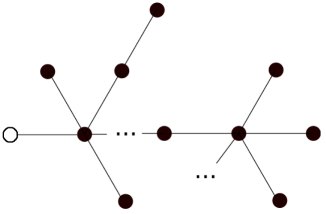
Figure 1: Theory graph of a general ghost-free multimetric theory. The black circles represent the $(N+1)$ metrics, the black lines represent pairwise interactions and the white circle represents the matter sector.

Clearly, the above restrictions still leave us with some freedom in constructing a multimetric model with $(N+1)$ fields. The case $N=0$ corresponds to GR with metric $g_{\mu\nu}$. There is a unique way to add a second tensor $f_{\mu\nu}$: it is coupled to $g_{\mu\nu}$ through an interaction of the form (3), resulting in the well-studied ghost-free bimetric theory. A third tensor field can now be added in two different ways: Either through a coupling to $g_{\mu\nu}$ or to $f_{\mu\nu}$. For $N>3$ fields, one can construct interaction diagrams of increasing complexity. This is illustrated in Figure 1. The only restriction on these graphs is that the lines representing pairwise interactions of the form (3) may never form a closed loop.

2.2 Models with maximal global symmetry

Due to the large number of possibilities for different multimetric theories, it would be useful to have a principle that singles out a certain class of preferred models. Here we demand the presence of global symmetries in the multimetric action. This will result in a simple class of multimetric models with a significantly smaller number of interaction parameters.

2.2.1 Interchange symmetry $S_{N}$

We are looking for multimetric theories with the maximum amount of discrete, global symmetries. One obvious symmetry of this type corresponds to the interchange of fields in a theory graph. Since the matter coupling necessarily breaks part of that symmetry by singling out a physical metric, the best one can achieve is a graph that is symmetric under the permutation of the remaining $N$ fields. The graph corresponding to a theory for which such a symmetry is possible is displayed in Figure 2.

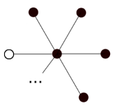
Figure 2: Theory graph of a multimetric theory with interchange symmetry among the $N$ satellite fields.

The action associated to this graph is of the form,

$$S[g,f^{(i)}]=m_{g}^{2}\int d^{4}x\Bigg{(}\sqrt{|g|} \,R(g)+\sum_{i=1}^{N}\alpha_{i}^{2}\sqrt{|f^{(i)}|}\,R(f^{(i)})$$

$$-2m^{2}\sum_{i=1}^{N}\sqrt{|g|}\,V(g,f^{(i)};\beta^{(i)}_{n})\Bigg{)}+S_{\mathrm{matter}}[g,\phi]\,.$$ (7)

The first line contains the Einstein-Hilbert kinetic terms for the tensor fields with “Planck masses” $m_{g}$ and $\alpha_{i}m_{g}$. The second line parameterises the interactions.

Requiring the invariance of the theory under the $S_{N}$ symmetry,

$$f_{\mu\nu}^{i}\longleftrightarrow f_{\mu\nu}^{j}\,,\qquad\forall~{}~{}i,j=1,\ldots,N\,,$$ (8)

restricts the interaction parameters in (2.2.1). The conditions on them can be derived as follows. After rescaling the satellite fields, $f_{\mu\nu}^{(i)}\rightarrow\tilde{f}_{\mu\nu}^{(i)}=\alpha_{i}^{-2}f_{\mu\nu}^{(i)}$, the Einstein-Hilbert terms are symmetric under interchange of $\tilde{f}_{\mu\nu}^{(i)}$ and $\tilde{f}_{\mu\nu}^{(j)}$. Since $e_{n}(\lambda S)=\lambda^{n}e_{n}(S)$ for a scalar $\lambda$, the potential is invariant only if one imposes,

$$\alpha^{-n}_{i}\beta^{(i)}_{n}=\alpha^{-n}_{j}\beta^{(j)}_{n}\qquad\forall~{}~{}i,j=1,\ldots,N\,.$$ (9)

These conditions imply that we are left with only five free interaction parameters, since we can now write $\beta^{(i)}_{n}=\alpha_{i}^{n}\beta_{n}$ for all $i$ with some fixed set of parameters $\beta_{n}$.

One may also consider slightly less symmetric examples where the interchange symmetry is only realised among $k$ out of the $N$ fields. This is the case when $\beta^{(i)}_{n}=\alpha_{i}^{n}\beta_{n}$ for $i=1,\ldots,k$ while the remaining $\beta^{(j)}_{n}$ remain arbitrary. Obviously, the discrete symmetry group in this case is $S_{k}$.

2.2.2 Reflection symmetry $(Z_{2})^{N}$

The maybe less obvious set of symmetries that one can demand in addition to the one in the previous subsection are the transformations,

$$\sqrt{g^{-1}f^{(i)}}\longrightarrow-\sqrt{g^{-1}f^{(i)}}\qquad\forall~{}~{}i=1,\ldots,N\,.$$ (10)

Given a square root $S$ as a solution to the equation $(S^{2})^{\mu}_{~{}\nu}=g^{\mu\rho}f_{\rho\nu}$, its negative counterpart $-S$ will also be a solution to the same equation. One way to implement the above transformation is to express the square-root matrix in terms of two constrained vierbeins $e^{a}_{~{}\mu}$ and $v^{a}_{~{}\mu}$ with $g_{\mu\nu}=\eta_{ab}e^{a}_{~{}\mu}e^{b}_{~{}\nu}$ and $f_{\mu\nu}=\eta_{ab}v^{a}_{~{}\mu}v^{b}_{~{}\nu}$. In terms of these we have,

$$S^{\mu}_{~{}\nu}=\big{(}\sqrt{g^{-1}f}\,\big{)}^{\mu}_{~{}\nu}=e_{b}^{~{}\mu}v^{b}_{~{}\nu}\,.$$ (11)

Now for each vierbein $(v^{(i)})^{b}_{~{}\nu}$ of $f_{\mu\nu}^{(i)}$, we consider the transformations,

$$(v^{(i)})^{b}_{~{}\nu}\longrightarrow-(v^{(i)})^{b}_{~{}\nu}\,,\qquad e^{a}_{~{}\mu}\longrightarrow e^{a}_{~{}\mu}\,,$$ (12)

which leave all metrics invariant but transforms the square roots according to (10). The Einstein-Hilbert terms are invariant since they contain the vierbeins only through their respective metrics. In the pairwise interactions the elementary symmetric polynomials transform as,

$$e_{n}(S)\longrightarrow(-1)^{n}e_{n}(S)\,.$$ (13)

Hence the potential is invariant only if we demand the odd terms to vanish,

$$\beta^{(i)}_{1}=\beta^{(i)}_{3}=0\qquad\forall~{}~{}i=1,\ldots,N\,.$$ (14)

It is again possible to impose a subset of symmetries by demanding (14) to hold for only $k$ of the $N$ parameter sets. In this case the action will be invariant under only $k$ transformations of the type (10) and the symmetry is $(Z_{2})^{k}$.

2.2.3 Maximally symmetric action

Imposing the conditions (9) and (14) results in the multimetric actions with maximal amount of global symmetry, $S_{N}\times(Z_{2})^{N}$. It reads,

$$S[g,f^{(i)}]=m_{g}^{2}\int d^{4}x\Bigg{(}\sqrt{|g|} \,R(g)+\sum_{i=1}^{N}\alpha_{i}^{2}\sqrt{|f^{(i)}|}\,R(f^{(i)})$$

$$-2m^{2}\sum_{i=1}^{N}\sqrt{|g|}\,V(g,f^{(i)};\alpha_{i}^{n}\beta_{n},)\Bigg{)}+S_{\mathrm{matter}}[g,\phi]\,,$$ (15)

where we have defined $\beta_{n}\equiv\alpha_{i}^{-n}\beta^{(i)}_{n}$ and the potentials now have the simple form,

$$\sqrt{|g|}\,V(g,f^{(i)};\alpha_{i}^{n}\beta_{n},) = \beta_{0}\sqrt{|g|}\,+\alpha_{i}^{2}\beta_{2}\sqrt{|g|}\,e_{2}\Big{(}\sqrt{g^{-1}f^{(i)}}\Big{)}+\alpha_{i}^{4}\beta_{4}\sqrt{|f^{(i)}|}\,\,,$$

$$e_{2}(S) = \frac{1}{2}\Big{(}S^{\rho}_{\phantom{\rho}\rho}S^{\sigma}_{\phantom{\sigma}\sigma}-S^{\rho}_{\phantom{\rho}\sigma}S^{\sigma}_{\phantom{\sigma}\rho}\Big{)}\,.$$ (16)

We see that $\beta_{0}$ and $\beta_{4}$ simply parameterise cosmological constant contributions and the only remaining interaction terms are proportional to $\beta_{2}$. To our knowledge there exist no further global symmetries that can be imposed on the gravitational part of the action (2.2.3).

3 Trimetric theory with maximal global symmetry

In this section we work out the details of a multimetric theory with maximal global symmetry. We specialise to three spin-2 fields to keep the expressions simple. The results obtained here naturally generalise to $N$ fields, as will be discussed in section 4.4.

The ghost-free action for three symmetric tensors $g_{\mu\nu}$, $f_{\mu\nu}$ and $h_{\mu\nu}$ with general parameters is of the form,

$$S[g,f,h]=m_{g}^{2}\int d^{4}x\Big{(} \sqrt{|g|}\,R(g)+\alpha_{f}^{2}\sqrt{|f|}\,R(f)+\alpha_{h}^{2}\sqrt{|h|}\,R(h)$$

$$-2m^{2}\sqrt{|g|}\,V(g,f;\beta_{n}^{f})-2m^{2}\sqrt{|g|}\,V(g,h;\beta_{n}^{h})\Big{)}+S_{\mathrm{matter}}[g,\phi]\,.$$ (17)

with potential as defined in (4). We will start by discussing its mass spectrum and explaining the physical effects of imposing the global symmetry which in this case is $S_{2}\times(Z_{2})^{2}\simeq Z_{2}\times(Z_{2})^{2}$.

3.1 Proportional backgrounds

In the following we review the mass spectrum of trimetric theory which has been derived in Baldacchino:2016jsz , generalising the bimetric results of Hassan:2012wr . We first need to find suitable maximally symmetric background solutions around which the fluctuations of the tensor fields can be diagonalised into mass eigenstates. These are the proportional backgrounds obtained by solving the equations of motion with the ansatz,

$$g_{\mu\nu}=c_{f}^{-2}f_{\mu\nu}=c_{h}^{-2}h_{\mu\nu}\,,$$ (18)

with two constants $c_{f}$ and $c_{h}$. In the following we denote the background metric by $\bar{g}_{\mu\nu}$. For the above ansatz, the equations of motion reduce to three copies of Einstein’s equations,

$$\mathcal{G}_{\mu\nu}(\bar{g})+\Big{(}\Lambda(\beta_{n}^{f},c_{f})+\Lambda(\beta_{n}^{h},c_{h})\Big{)}\bar{g}_{\mu\nu} = 0\,,$$ (19a)

$$\mathcal{G}_{\mu\nu}(\bar{g})+\tilde{\Lambda}(\beta_{n}^{f},c_{f},\alpha_{f})\bar{g}_{\mu\nu} = 0\,,$$ (19b)

$$\mathcal{G}_{\mu\nu}(\bar{g})+\tilde{\Lambda}(\beta_{n}^{h},c_{h},\alpha_{h})\bar{g}_{\mu\nu} = 0\,,$$ (19c)

where $\mathcal{G}_{\mu\nu}(\bar{g})$ is the Einstein tensor of the metric $\bar{g}_{\mu\nu}$ and,

$$\Lambda(\beta_{n},c) = m^{2}\left(\beta_{0}+3c\beta_{1}+3c^{2}\beta_{2}+c^{3}\beta_{3}\right)\,,$$ (20)

$$\tilde{\Lambda}(\beta_{n},c,\alpha) = \frac{m^{2}}{\alpha^{2}c^{2}}\left(c\beta_{1}+3c^{2}\beta_{2}+3c^{3}\beta_{3}+c^{4}\beta_{4}\right)\,.$$ (21)

Since the Einstein tensor is scale-invariant one finds the two background conditions,

$$\Lambda(\beta_{n}^{f},c_{f})+\Lambda(\beta_{n}^{h},c_{h})=\tilde{\Lambda}(\beta_{n}^{f},c_{f},\alpha_{f})=\tilde{\Lambda}(\beta_{n}^{h},c_{h},\alpha_{h})\,.$$ (22)

These determine the proportionality constants $c_{f}$ and $c_{h}$ in terms of the parameters of the theory. For an action with $S_{2}\times(Z_{2})^{2}$ symmetry, all solutions satisfy,

$$\alpha_{f}^{2}c_{f}^{2}=\alpha_{h}^{2}c_{h}^{2}\,.$$ (23)

Since all cosmological constant contributions in (19) are equal, we will simply refer to them by the symbol $\Lambda$.

3.2 Mass eigenstates

Next one derives the equations of motion for linear perturbations of the metrics around the proportional backgrounds, $g_{\mu\nu}=\bar{g}_{\mu\nu}+\delta g_{\mu\nu}$, $f_{\mu\nu}=c_{f}^{2}\bar{g}_{\mu\nu}+\delta f_{\mu\nu}$, and $h_{\mu\nu}=c_{h}^{2}\bar{g}_{\mu\nu}+\delta h_{\mu\nu}$. The equations will not be diagonal in these fluctuations and hence the latter do not correspond to the mass eigenstates of the theory. In order to find the eigenstates one solves the characteristic equation of the mass matrix. For interaction parameters that satisfy the condition (9) and (14) and thereby realise the $S_{2}\times(Z_{2})^{2}$ invariance of the action, the canonically normalised eigenstates of the mass matrix assume the following simple form,

$$\delta G_{\mu\nu} = \frac{m_{\mathrm{Pl}}\left(\delta g_{\mu\nu}+\alpha_{f}^{2}\delta f_{\mu\nu}+\alpha_{h}^{2}\delta h_{\mu\nu}\right)}{1+\alpha_{f}^{2}c_{f}^{2}+\alpha_{h}^{2}c_{h}^{2}}\,,$$ (24a)

$$\delta{M}_{\mu\nu} = \frac{{m_{\mathrm{Pl}}}\left(\alpha_{f}^{2}\delta f_{\mu\nu}+\alpha_{h}^{2}\delta h_{\mu\nu}-(\alpha_{f}^{2}c_{f}^{2}+\alpha_{h}^{2}c_{h}^{2})\delta g_{\mu\nu}\right)}{(1+\alpha_{f}^{2}c_{f}^{2}+\alpha_{h}^{2}c_{h}^{2})\sqrt{\alpha_{f}^{2}c_{f}^{2}+\alpha_{h}^{2}c_{h}^{2}}}\,,$$ (24b)

$$\delta\chi_{\mu\nu} = \frac{{m_{\mathrm{Pl}}}{\alpha_{f}\alpha_{h}}\left(\frac{c_{f}}{c_{h}}\delta h_{\mu\nu}-\frac{c_{h}}{c_{f}}\delta f_{\mu\nu}\right)}{\sqrt{1+\alpha_{f}^{2}c_{f}^{2}+\alpha_{h}^{2}c_{h}^{2}}\sqrt{\alpha_{f}^{2}c_{f}^{2}+\alpha_{h}^{2}c_{h}^{2}}}\,,$$ (24c)

where we have defined the physical Planck mass,

$$m_{\mathrm{Pl}}\equiv m_{g}\sqrt{1+\alpha_{f}^{2}c_{f}^{2}+\alpha_{h}^{2}c_{h}^{2}}\,.$$ (25)

Note in particular that the state $\delta\chi_{\mu\nu}$ is independent of the original fluctuation $\delta g_{\mu\nu}$. The corresponding mass eigenvalues are given by,

$$\mu_{G}^{2}=0\,,\qquad\mu_{M}^{2}=\mathcal{A}(1+\alpha_{f}^{2}c_{f}^{2}+\alpha_{h}^{2}c_{h}^{2})m^{2}\,,\qquad\mu_{\chi}^{2}=\mathcal{A}m^{2}\,.$$ (26)

with $\mathcal{A}\equiv\frac{2\beta_{f}^{2}}{\alpha_{f}^{2}}=\frac{2\beta_{h}^{2}}{\alpha_{h}^{2}}$. Using the background condition (23), the mass eigenstates can be written in the form,

$$\delta G_{\mu\nu} = \frac{m_{\mathrm{Pl}}\left(\delta g_{\mu\nu}+\alpha_{f}^{2}\delta f_{\mu\nu}+\alpha_{h}^{2}\delta h_{\mu\nu}\right)}{1+\alpha^{2}}\,,$$ (27a)

$$\delta{M}_{\mu\nu} = \frac{{m_{\mathrm{Pl}}}\left(\alpha_{f}^{2}\delta f_{\mu\nu}+\alpha_{h}^{2}\delta h_{\mu\nu}-\alpha^{2}\delta g_{\mu\nu}\right)}{\alpha(1+\alpha^{2})}\,,$$ (27b)

$$\delta\chi_{\mu\nu} = \frac{{m_{\mathrm{Pl}}}\left(\alpha_{h}^{2}\delta h_{\mu\nu}-\alpha_{f}^{2}\delta f_{\mu\nu}\right)}{\alpha\sqrt{1+\alpha^{2}}}\,,$$ (27c)

where we have defined,

$$\alpha^{2}\equiv\alpha_{f}^{2}c_{f}^{2}+\alpha_{h}^{2}c_{h}^{2}=2\alpha_{f}^{2}c_{f}^{2}=2\alpha_{h}^{2}c_{h}^{2}\,.$$ (28)

The quadratic action in terms of mass eigenstates is provided in appendix A.

Let us comment on some immediate phenomenological implications. The spin-2 mass eigenstate $\delta\chi_{\mu\nu}$ does not interact directly with the matter sector since the matter coupling contains only the fluctuations of the physical metric $g_{\mu\nu}$. For instance, the coupling in the quadratic action is of the form,

$$\delta g^{\mu\nu}T_{\mu\nu}=\frac{1}{m_{\mathrm{Pl}}}\left(\delta G^{\mu\nu}-\alpha\,\delta{M}^{\mu\nu}\right)T_{\mu\nu}\,,$$ (29)

where $T_{\mu\nu}$ is the matter stress-energy tensor (here taken to be a small fluctuation sourcing perturbations on the proportional backgrounds). Matter couplings involving $\delta\chi_{\mu\nu}$ are forbidden by the global symmetries. Note furthermore from (26) that the mass of $\delta{M}_{\mu\nu}$ is always larger than that of $\delta\chi_{\mu\nu}$ by a factor of $\sqrt{1+\alpha^{2}}$. The particle corresponding to $\delta\chi_{\mu\nu}$ is thus stable against two-body decay into SM particles and other massive spin-2 modes. In fact, these decay diagrams are also forbidden by the global symmetries, as we will explain in section 4.3. Namely, the symmetries forbid all linear couplings in $\delta\chi_{\mu\nu}$ and hence higher-order decays (such as $\delta\chi\rightarrow 2\delta M\rightarrow 4\,$SM) with off-shell spin-2 modes are not possible either. Moreover, in the next section we will demonstrate that $\delta\chi_{\mu\nu}$ does not decay into massless gravitons and is therefore entirely stable. A decay of the heavier spin-2 particle into two lighter ones, $\delta{M}\rightarrow\delta\chi\delta\chi$, is possible provided that $\mu_{M}>2\mu_{\chi}$. Since $\mu_{M}^{2}=(1+\alpha^{2})\mu^{2}_{\chi}$ this requires $\alpha^{2}>3$. A decay into one massive and any number of massless particles, $\delta{M}\rightarrow\delta\chi\delta G\delta G\ldots$, is again forbidden by the global symmetries.

In section 4.4 we will see that all of these results naturally generalise to theories with $N$ satellite fields and symmetry $S_{N}\times(Z_{2})^{N}$.

4 Perturbative expansion of the action

In this section we discuss the perturbative expansion of the trimetric action with maximal symmetry in terms of mass eigenstates. Inverting the relations (27), we can express the original metric fluctuations in terms of the mass eigenstates as follows,

$$\delta g_{\mu\nu} = \frac{1}{m_{\mathrm{Pl}}}\left(\delta G_{\mu\nu}-\alpha\,\delta{M}_{\mu\nu}\right)\,,$$ (30a)

$$\delta f_{\mu\nu} = \frac{\alpha}{2\alpha_{f}^{2}m_{\mathrm{Pl}}}\left(\alpha\delta G_{\mu\nu}-\sqrt{1+\alpha^{2}}\delta\chi_{\mu\nu}+\delta M_{\mu\nu}\right)\,,$$ (30b)

$$\delta h_{\mu\nu} = \frac{\alpha}{2\alpha_{h}^{2}m_{\mathrm{Pl}}}\left(\alpha\delta G_{\mu\nu}+\sqrt{1+\alpha^{2}}\delta\chi_{\mu\nu}+\delta M_{\mu\nu}\right)\,.$$ (30c)

These expression can now be used to compute the interaction vertices of mass eigenstates to all orders in the trimetric action (3) with parameters satisfying the conditions (9) and (14).

For $\alpha<1$, the scale suppressing higher-order vertices of $\delta M$ and $\delta\chi$ is $\alpha m_{\mathrm{Pl}}$. The perturbative structure is thus formally the same as in bimetric theory where $\alpha$ was simply the ratio of two Planck masses. It was discussed in detail in Babichev:2016bxi that in this case the perturbative expansion is valid for energies smaller than $\alpha m_{\mathrm{Pl}}$.

4.1 Nonlinear massless field

Just like in the bimetric case (see Babichev:2016bxi ), it is possible to define a nonlinear massless metric,

$$G_{\mu\nu}=\bar{g}_{\mu\nu}+\frac{1}{m_{\mathrm{Pl}}}\delta G_{\mu\nu}\,.$$ (31)

In terms of this, we can then write the full metrics $g_{\mu\nu}$, $f_{\mu\nu}$ and $h_{\mu\nu}$ as follows,

$$g_{\mu\nu} = G_{\mu\nu}-\frac{\alpha}{m_{\mathrm{Pl}}}\delta{M}_{\mu\nu}\,,$$ (32a)

$$f_{\mu\nu} = \frac{\alpha^{2}}{2\alpha_{f}^{2}}G_{\mu\nu}+\frac{\alpha}{2\alpha_{f}^{2}m_{\mathrm{Pl}}}\left(\delta M_{\mu\nu}-\sqrt{1+\alpha^{2}}\,\delta\chi_{\mu\nu}\right)\,,$$ (32b)

$$h_{\mu\nu} = \frac{\alpha^{2}}{2\alpha_{h}^{2}}G_{\mu\nu}+\frac{\alpha}{2\alpha_{h}^{2}m_{\mathrm{Pl}}}\left(\delta M_{\mu\nu}+\sqrt{1+\alpha^{2}}\,\delta\chi_{\mu\nu}\right)\,.$$ (32c)

The field $G_{\mu\nu}$ is massless in the following sense. If we insert the expressions (32) back into (3) and formally neglect the massive modes by setting $\delta M_{\mu\nu}=\delta\chi_{\mu\nu}=0$, we recover the Einstein-Hilbert action for $G_{\mu\nu}$,

$$\left.S[g,f,h]\right|_{\delta M=\delta\chi=0}=m_{\mathrm{Pl}}^{2}\int\mathrm{d}^{4}x~{}\sqrt{|G|}\,\left(R(G)-2\Lambda\right)\,,$$ (33)

where $\Lambda$ is identical to the cosmological constant of the background metric $\bar{g}_{\mu\nu}$. The self-interactions of $G_{\mu\nu}$ are exactly the same as those of the massless tensor field in GR. Even at the nonlinear level, we can therefore interpret the fluctuation $\delta G_{\mu\nu}$ as the massless field mediating the long-ranged gravitational force, and the metric $G_{\mu\nu}$ sets the geometry in which the massive spin-2 modes propagate.

4.2 Vertices linear in both massive modes

Next we study the vertices linear in the massive modes, i.e. we expand the trimetric action (3) to linear order in $\delta M_{\mu\nu}$ and $\delta\chi_{\mu\nu}$, formally keeping all orders of $G_{\mu\nu}$. This gives an all-order result but neglects vertices including more than one massive mode. The contributions from the Einstein-Hilbert terms are,

$$m_{g}^{2}\int d^{4}x\left.\tfrac{\delta\sqrt{|g|}\,R(g)}{\delta g_{\mu\nu}}\right|_{g=G}\left(\delta g_{\mu\nu}+\alpha_{f}^{2}\delta f_{\mu\nu}+\alpha_{h}^{2}\delta h_{\mu\nu}\right)$$ (34)

$$=~{} \tfrac{m_{g}^{2}}{m_{\mathrm{Pl}}}\int d^{4}x\left.\tfrac{\delta\sqrt{|g|}\,R(g)}{\delta g_{\mu\nu}}\right|_{g=G}\left[\Big{(}\tfrac{\alpha_{f}^{2}c_{f}^{2}}{\alpha}+\tfrac{\alpha_{h}^{2}c_{h}^{2}}{\alpha}-\alpha\Big{)}\delta M_{\mu\nu}+\tfrac{\sqrt{1+\alpha^{2}}}{\alpha}\Big{(}\alpha_{h}^{2}c_{h}^{2}-\alpha_{f}^{2}c_{f}^{2}\Big{)}\delta\chi_{\mu\nu}\right]\,.$$ (35)

Since $\alpha^{2}=\alpha_{h}^{2}c_{h}^{2}+\alpha_{f}^{2}c_{f}^{2}$ and $\alpha_{h}^{2}c_{h}^{2}=\alpha_{f}^{2}c_{f}^{2}$, the round brackets in the last line both vanish and hence there are no vertices linear in the massive modes coming from the Einstein-Hilbert terms. Taylor expansion of the interaction potential $\sqrt{|g|}\,V=\sqrt{|g|}\,(V(g,f;\beta_{n}^{f})+V(g,h;\beta_{n}^{h}))$ to first order around the proportional backgrounds gives rise to the following couplings,

$$~{}m^{2}\left.\tfrac{\partial(\sqrt{|g|}\,V)}{\partial\delta\chi_{\rho\sigma}}\right|_{f=h=g=G}\delta\chi_{\rho\sigma}+m^{2}\left.\tfrac{\partial(\sqrt{|g|}\,V)}{\partial\delta M_{\rho\sigma}}\right|_{f=h=g=G}\delta M_{\rho\sigma}$$

$$= \left[\tfrac{\partial(\sqrt{|g|}V(g,f;\beta^{f}_{n}))}{\partial f^{\mu\nu}}\tfrac{\partial f^{\mu\nu}}{\partial\delta\chi_{\rho\sigma}}+\tfrac{\partial(\sqrt{|g|}V(g,h;\beta^{h}_{n}))}{\partial h^{\mu\nu}}\tfrac{\partial h^{\mu\nu}}{\partial\delta\chi_{\rho\sigma}}\right]_{f=h=g=G}\delta\chi_{\rho\sigma}$$

$$+\left[\tfrac{\partial(\sqrt{|g|}V)}{\partial g^{\mu\nu}}\tfrac{\partial g^{\mu\nu}}{\partial\delta{M}_{\rho\sigma}}+\tfrac{\partial(\sqrt{|g|}V(g,f;\beta^{f}_{n}))}{\partial f^{\mu\nu}}\tfrac{\partial f^{\mu\nu}}{\partial\delta{M}_{\rho\sigma}}+\tfrac{\partial(\sqrt{|g|}V(g,h;\beta^{h}_{n}))}{\partial h^{\mu\nu}}\tfrac{\partial h^{\mu\nu}}{\partial\delta{M}_{\rho\sigma}}\right]_{f=h=g=G}\delta M_{\rho\sigma}$$

$$\equiv~{} \tfrac{\sqrt{1+\alpha^{2}}}{2\alpha}\tilde{\Lambda}(\beta^{f}_{n},c_{f},\alpha_{f})\Big{(}\alpha_{h}^{2}c_{h}^{2}-\alpha_{f}^{2}c_{f}^{2}\Big{)}\sqrt{|G|}\,G^{\rho\sigma}\delta\chi_{\rho\sigma}$$

$$+\tfrac{1}{2}\tilde{\Lambda}(\beta^{f}_{n},c_{h},\alpha_{f})\Big{(}\tfrac{\alpha_{f}^{2}c_{f}^{2}}{\alpha}+\tfrac{\alpha_{h}^{2}c_{h}^{2}}{\alpha}-\alpha\Big{)}\sqrt{|G|}\,G^{\rho\sigma}\delta M_{\rho\sigma}\,.$$ (36)

where we have evaluated the variations of the potential terms on the background and used (22) and (32). The expressions in the round brackets again vanish and the interaction potential does not contain linear fluctuations in the massive modes either.

4.3 Cubic vertices

We now obtain the expression for the perturbed trimetric action to cubic order in mass eigenstates. Our full and explicit results can be found in appendix A. In Table 1 we collect the pre-factors of cubic interaction vertices, paying particular attention to the dependence on $\alpha$, but neglecting numerical factors. Dimensionless factors always multiply kinetic interactions.

Table 1: Prefactors of cubic vertices; all suppressed by $m_{\mathrm{Pl}}^{-1}$.

		$\delta\chi^{3}$, $\delta G^{2}\delta M$,
$\delta G^{3}$	$\delta M^{3}$	$\delta G^{2}\delta\chi$, $\delta M^{2}\delta\chi$	$\delta M^{2}\delta G$	$\delta\chi^{2}\delta G$	$\delta\chi^{2}\delta M$
$1,\Lambda$	$\frac{1-\alpha^{2}}{\alpha}\cdot(1,\Lambda,\mu_{M}^{2})$	$0$	$1,\Lambda,\mu_{M}^{2}$	$1,\Lambda,\mu_{\chi}^{2}$	$\frac{1}{\alpha}\cdot(1,\Lambda,\mu_{M}^{2},\mu_{\chi}^{2})$

We notice a couple of distinct features.

• The cubic self-interactions of the massless mode $\delta G_{\mu\nu}$ are exactly those of GR, which is consistent with the all-order results of section 4.1.

• As expected from the general results derived in section 4.2, there are no terms linear in both $\delta M_{\mu\nu}$ and $\delta\chi_{\mu\nu}$. This explicitly confirms that the cubic vertices do not give rise to diagrams describing decay into massless gravitons.

• The cubic action does not contain terms with odd powers of $\delta\chi_{\mu\nu}$. In fact, this holds to all orders in perturbation series which can be seen as follows. Under the interchange symmetry $\alpha_{f}^{2}f_{\mu\nu}\leftrightarrow\alpha_{h}^{2}h_{\mu\nu}$, which leaves the action invariant, this mode transforms as $\delta\chi_{\mu\nu}\rightarrow-\delta\chi_{\mu\nu}$, whereas the other two mass eigenstates are invariant, $\delta M_{\mu\nu}\rightarrow\delta M_{\mu\nu}$ and $\delta G_{\mu\nu}\rightarrow\delta G_{\mu\nu}$. Hence, a term with odd powers of $\delta\chi_{\mu\nu}$ would transform into its negative and spoil the invariance of the action. It can therefore not exist. Consequently a decay into one massive and any number of massless particles, $\delta{M}\rightarrow\delta\chi\delta G\delta G\ldots$, is forbidden because it requires a vertex that is linear in $\delta\chi_{\mu\nu}$.

• The vertices with two massive and one massless mode do not depend on $\alpha$. This is expected because they will enter the expression for the gravitational stress-energy tensor, which coincides with the Noether stress-energy defined for the ($\alpha$-independent) quadratic action in flat space Leclerc:2005na .

• All of the cubic self-interactions of $\delta M_{\mu\nu}$ are enhanced for both small and large $\alpha$, but with opposite sign. Interestingly, they all vanish for $\alpha^{2}=1$.

• All $\delta M\delta\chi\delta\chi$ terms are enhanced for small $\alpha$. On the other hand, while everything is naturally Planck scale suppressed, with a large value for $\alpha$ the suppression of these terms would be even stronger.

4.4 Generalisation to multiple fields

The mass spectrum of a general multimetric theory is rather complicated. For a theory of the form (2.2.1) it has been worked out explicitly in Baldacchino:2016jsz . The mass eigenstates are linear combinations of the metric fluctuations $\delta g_{\mu\nu}$ and $\delta f_{\mu\nu}^{(i)}$ around a maximally symmetric background solution. The spectrum always contains one massless mode $\delta G_{\mu\nu}$ and $N$ massive modes $\delta\chi^{(i)}_{\mu\nu}$ with masses $\mu_{i}$.

From the results of Baldacchino:2016jsz we can derive a feature shared by all models with at least one discrete interchange symmetry of section 2.2.1 and two reflection symmetries of section 2.2.2: When the conditions (9) and (14) are imposed on the same two parameter sets, then in one of the massive states $\delta\chi^{(i)}_{\mu\nu}$ the coefficient in front of $\delta g_{\mu\nu}$ vanishes and hence this massive mode drops out of the matter coupling.

In particular, for the action (2.2.3) with maximal symmetry $S_{N}\times(Z_{2})^{N}$, the proportional backgrounds $f_{\mu\nu}^{i}=c_{i}^{2}g_{\mu\nu}$ satisfy $c_{i}^{2}/c_{j}^{2}=\alpha_{j}^{2}/\alpha_{i}^{2}$ and the mass spectrum takes on the form,

$$\delta G_{\mu\nu} = \frac{m_{\mathrm{Pl}}}{1+\alpha^{2}}\left(\delta g_{\mu\nu}+\sum_{k=1}^{N}\alpha_{k}^{2}\delta f^{(k)}_{\mu\nu}\right)\,,$$ (37a)

$$\delta{M}_{\mu\nu} = \frac{{m_{\mathrm{Pl}}}}{(1+\alpha^{2})\alpha}\left(\sum_{k=1}^{N}\alpha_{k}^{2}\delta f^{(k)}_{\mu\nu}-\alpha^{2}\delta g_{\mu\nu}\right)\,,$$ (37b)

$$\delta\chi^{(i)}_{\mu\nu} = \frac{m_{\mathrm{Pl}}}{\alpha\sqrt{1+\alpha^{2}}}\left(\alpha_{i}^{2}\delta f^{(i)}_{\mu\nu}-\alpha_{i+1}^{2}\delta f^{(i+1)}_{\mu\nu}\right)\qquad i=1,\dots,N-1\,.$$ (37c)

with $\alpha^{2}=\sum_{k=1}^{N}\alpha_{k}^{2}c_{k}^{2}$ and $m_{\mathrm{Pl}}=\sqrt{1+\alpha^{2}}\,m_{g}$. One mode (which we have labelled $\delta M_{\mu\nu}$) retains its dependence on $\delta g_{\mu\nu}$ because imposing the full $S_{N}$ invariance gives only $(N-1)$ conditions of the form (9). Since the fields $\delta\chi^{(i)}_{\mu\nu}$ do not depend on the fluctuation $\delta g_{\mu\nu}$ of the physical metric, they do not show up in the coupling to matter. Their masses $\mu_{i}$ are all equal to each other and related to the mass ${\mu}_{M}$ of $\delta M_{\mu\nu}$ through,

$$\mu_{i}=\mu_{j}=\frac{{\mu}_{M}}{\sqrt{1+\alpha^{2}}}\qquad\forall~{}i,j=1,\dots,N-1\,.$$ (38)

As in the trimetric case, we derive from (37) that,

$$\delta g_{\mu\nu}=\frac{1}{m_{\mathrm{Pl}}}\left(\delta G_{\mu\nu}-\alpha\,\delta{M}_{\mu\nu}\right)\,.$$ (39)

Matter thus only interacts with the massless and with the heaviest spin-2 field while the $(N-1)$ massive spin-2 particles corresponding to the modes $\delta\chi^{(i)}_{\mu\nu}$ cannot decay into SM particles. Moreover, they all have equal mass and are lighter than $\delta{M}_{\mu\nu}$, which forbids the two-body decay into massive spin-2 particles. Higher order decay channels are again forbidden by the global symmetries which ensure the absence of terms linear in $\delta\chi^{(i)}_{\mu\nu}$. The only remaining decay channel would be into massless gravitons but the generalisation of the calculation in section 4.2 shows that there are no couplings giving rise to such decay diagrams.

5 Dark matter phenomenology

The absolute stability of the lightest mode $\delta\chi_{\mu\nu}$ motivates us to consider it as a possible candidate for the DM particle. Before exploring the phenomenological implications of this idea, we make a few comments on how we restrict the ranges for the parameters of maximally symmetric trimetric theory.

5.1 Parameter regions of interest

The particle corresponding to the massive spin-2 mode $\delta\chi_{\mu\nu}$ is completely stable since it does not decay into massive spin-2 fields $\delta M_{\mu\nu}$, nor massless gravitons $\delta G_{\mu\nu}$ and it does not couple to Standard Model fields. Even without any global symmetries in the action, the lightest spin-2 mode would not decay into $\delta G_{\mu\nu}$, since this coupling does not arise in any diffeomorphism invariant theory. The decay into SM matter on the other hand is forbidden by the global $S_{2}\times(Z_{2})^{2}$ symmetry of the theory. We expect (but do not prove) that both the diffeomorphism invariance and the global symmetry are stable under quantum corrections. Provided that this is correct, no parameters need to be tuned in order to guarantee the stability of the particle corresponding to $\delta\chi_{\mu\nu}$.

The Planck mass $m_{\mathrm{Pl}}$ is known to be large, on the order of $10^{18}$ GeV, giving rise to feeble gravitational interactions. This creates the well-known hierarchy between the Planck scale and the weak scale. Moreover, the cosmological constant $\Lambda$ is measured to be very small, $\Lambda\simeq 10^{-122}m_{\mathrm{Pl}}^{2}$. We do not attempt to address these hierarchy problems here, but tune the values of $m_{\mathrm{Pl}}$ and $\Lambda$ to match the gravitational and cosmological observations.

We need to make an assumption on the dimensionless parameter $\alpha$ that parameterises the interaction strengths of massive spin-2 modes. It is obvious that the limit $\alpha^{2}=\alpha_{f}^{2}c_{f}^{2}+\alpha_{h}^{2}c_{h}^{2}\rightarrow 0$ is the generalisation of the GR limit $\alpha\rightarrow 0$ in bimetric theory Baccetti:2012bk ; Hassan:2014vja . More precisely, in the bimetric case it is known that the parameter $\alpha$ and the spin-2 mass $m$ together control the deviations from GR Babichev:2016bxi . Demanding $\alpha\ll 1$ ensures that these deviations are small for a large range of spin-2 masses (and in particular small ones). It is easy to see that the situation will be similar in the presence of multiple massive spin-2 fields and we take this as a motivation to begin our investigations by focusing on values $\alpha^{2}=\alpha_{f}^{2}c_{f}^{2}+\alpha_{h}^{2}c_{h}^{2}<1$ in this work. We will comment on the interesting implications of larger values for $\alpha$ in section 6.

One important implication of the assumption $\alpha<1$ is that the masses of the spin-2 modes in (26) are of the same order, $\mu_{M}\simeq\mu_{\chi}$. In this case $\delta M_{\mu\nu}$ cannot decay into $\delta\chi_{\mu\nu}$ since $2\mu_{\chi}>\mu_{M}$. We take $\beta^{f}_{2}=\alpha_{h}^{2}\beta_{2}^{h}/\alpha_{f}^{2}$ to be of order unity and hence $\mu_{M}\simeq\mu_{\chi}\simeq m$. The heaviest mode can of course still decay into Standard Model fields and its matter coupling is of the same form as in bimetric theory. It then follows from the results of Babichev:2016bxi that if $\delta M_{\mu\nu}$ makes up (part of) the observed dark matter density, its non-observation in indirect detection experiments requires $10^{-15}\lesssim\alpha\lesssim 10^{-12}$ and $m\simeq 1-100$ TeV. In other words, the bimetric DM scenario with freeze-in production mechanism can also be realised in the presence of more than one massive spin-2 particle and, since the lighter field $\delta\chi_{\mu\nu}$ is not observable in indirect detection experiments, the phenomenology will essentially be the same.

Interestingly, the multimetric theory leaves us with more options. Namely we can require that $\delta M_{\mu\nu}$ does not contribute to the observed dark matter density because it has decayed since the end of inflation. This basically provides us with the reversed stability bound derived in Babichev:2016bxi ,

$$\alpha^{2/3}\mu_{M}>0.13\,\mathrm{GeV}\,.$$ (40)

For fixed spin-2 mass, this translates into a lower bound on $\alpha$. For instance, for $\mu_{M}\simeq 1$ TeV we need $\alpha>10^{-6}$. Without an abundance of $\delta M_{\mu\nu}$ particles, there are no constraints from indirect detection experiments forcing $\alpha$ to be small. In fact, as we will mention in section 5.3, such constraints seem to favour larger values for $\alpha$. Let us emphasise once more that this has no effect on the stability of the lighter spin-2 field $\delta\chi_{\mu\nu}$ which is our dark matter candidate. In what follows we will always impose the bound (40), keeping in mind that there exists another region in parameters space with much smaller $\alpha$ where the analogue of the bimetric DM scenario could be at work.

5.2 Production mechanisms for $\alpha<1$

The assumptions motivated in the previous section can be summarised as,

$$\left(\frac{0.13\,\mathrm{GeV}}{\mu_{M}}\right)^{3/2}<\alpha<1\,,\qquad\beta^{f}_{2}=\frac{\alpha_{h}^{2}\beta_{2}^{h}}{\alpha_{f}^{2}}\simeq 1\,,\qquad\Rightarrow~{}~{}\mu_{M}\simeq\mu_{\chi}\simeq m\,.$$ (41)

DM related observations now essentially constrain the remaining parameters $\alpha$ and $m$.

In Babichev:2016bxi it was explained why the freeze-out mechanism cannot be responsible for the production of massive spin-2 dark matter. This is due to the Planck suppression of the coupling between $\delta M_{\mu\nu}$ and matter fields, which does not allow the two sectors to reach thermal equilibrium in the early Universe. The same issue arises in multimetric theory (at least for $\alpha<1$) and we have to rely on different production mechanisms for spin-2 dark matter. In the following we argue that both freeze-in Hall:2009bx and gravitational particle production Chung:1998zb ; Kuzmin:1998uv ; Chung:2004nh can yield the observed dark matter abundance.

5.2.1 Scenario I: Freeze-in production

Even though the massive spin-2 sector does not attain thermal equilibrium with matter particles in the early Universe, a relic density can be produced through a slow “leakage” from the thermal bath, resulting in a non-thermalised DM sector Hall:2009bx . In our case two Standard Model particles from the thermal bath annihilate and produce a pair of massive spin-2 particles via $s$-channel exchange of $\delta G_{\mu\nu}$ or $\delta M_{\mu\nu}$. This very slow process is never counterbalanced by the opposite one because the abundance of massive spin-2 always remains well below the thermal one. The production can take place during reheating or in the radiation dominated era thereafter Garny:2015sjg ; Tang:2016vch .

The end products of the $s$-channel production are pairs of spin-2 particles corresponding to either $\delta M_{\mu\nu}$ or $\delta\chi_{\mu\nu}$ (with approximately equal masses $m$). A $\delta M\delta\chi$ pair is not possible due to the absence of couplings linear in $\delta\chi_{\mu\nu}$ (c.f. the discussion in section 4.3). The dominant Feynman diagrams contain the linear matter coupling and a cubic interaction vertex (here we use the approximation $1+\alpha^{2}\simeq 1$):

Production of a $\delta M\delta M$ or a $\delta\chi\delta\chi$ pair via $s$-channel exchange of $\delta G$.	Production of a $\delta M\delta M$ or a $\delta\chi\delta\chi$ pair via $s$-channel exchange of $\delta M$.

They all contribute equally and are independent of $\alpha$. In principle now both the $\delta M_{\mu\nu}$ and $\delta\chi_{\mu\nu}$ particles could contribute to the DM abundance. However, as explained in the previous subsection, if the $\delta M_{\mu\nu}$ particle made up part of DM then this would force $\alpha$ to be very tiny and essentially bring us back to the bimetric scenario. We therefore restrict to parameters that satisfy the bound (40) such that most of the $\delta M_{\mu\nu}$ particles have decayed over the age of the universe and we are left with the entirely stable DM particle $\delta\chi_{\mu\nu}$ alone.

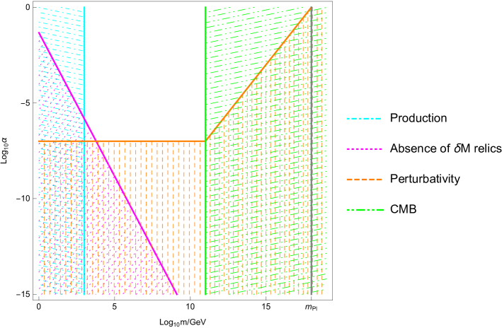
Figure 3: Excluded regions in the $m$-$\alpha$-plane for freeze-in production.

The allowed mass region for $m_{\chi}\simeq m$ is the same as in the bimetric case before imposing the constraints from indirect detection Babichev:2016bxi ,

$$1\,\mathrm{TeV}\lesssim m\lesssim 10^{11}\,\mathrm{GeV}\,.$$ (42)

The lower bound stems from demanding the observed DM abundance to be generated during either reheating or radiation domination. It is sensitive to the efficiency of the reheating process, $\epsilon_{\mathrm{rh}}=\frac{\pi^{2}g_{*}T^{4}_{\mathrm{rh}}}{90m_{\mathrm{Pl}}^{2}H_{e}^{2}}\leq 1$, with reheating temperature $T_{\mathrm{rh}}$, Hubble scale at the end of inflation $H_{e}$ and $g_{*}=106.75$ being the number of relativistic degrees of freedom during reheating. The displayed bound corresponds to maximal efficiency. For lower values of $\epsilon_{\mathrm{rh}}$, the bound on the mass moves to higher values. The upper bound is essentially a constraint on the scale of inflation from non-observation of tensor modes in the CMB.

The allowed values for $\alpha$ are obtained by demanding the absence of a relic density of $\delta M_{\mu\nu}$ particles and validity of the perturbative expansion. They can be read off from Figure 3. The perturbativity bound is a combination of demanding $m<\alpha m_{\mathrm{Pl}}$ and $T_{\mathrm{rh}}<\alpha m_{\mathrm{Pl}}$, where for the latter we have assumed the minimal value required for efficient production, $T_{\mathrm{rh}}\simeq 10^{-7}m_{\mathrm{Pl}}$ Tang:2016vch .

5.2.2 Scenario II: Gravitational production

Another possible origin of a relic density of stable, massive spin-2 particles is the non-adiabatic transition of the Universe out of its de-Sitter phase at the end of inflation. This change in the cosmological expansion induces a non-adiabatic change in the frequencies of the Fourier modes defining the particles. This in turn leads to mixing between modes with positive and negative frequency and thus to quantum creation of particles. The mechanism, known as gravitational particle production, is effective only for very heavy masses, for details see Chung:1998zb ; Kuzmin:1998uv ; Chung:2004nh .

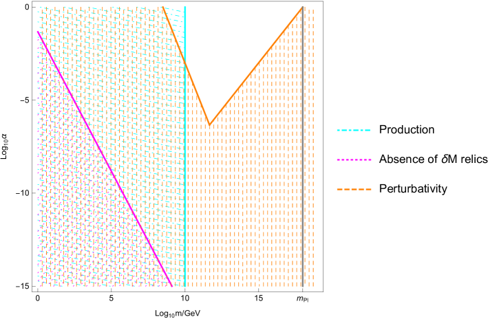
Figure 4: Excluded regions in the $m$-$\alpha$-plane for gravitational particle production.

The bimetric scenario of Babichev:2016bxi excluded it as a possible mechanism generating the non-thermal relic density by invoking constraints on isocurvature perturbations. Namely, these translated into a lower limit for the spin-2 mass,

$$m\gtrsim 10^{10}\,\mathrm{GeV}\,,$$ (43)

which together with constraints from indirect detection experiments resulted in a very low upper bound on the analogue of the parameter $\alpha$ in the bimetric case. Such a small $\alpha$ was inconsistent with perturbativity. In contrast, in the multimetric case, the DM particle does not decay and hence the constraints from indirect detection are irrelevant, provided that (40) holds. Together, (40) and (43) now give a very weak lower bound on $\alpha$ instead, namely $\alpha\gtrsim 10^{-16}$. The requirement of perturbativity, $m\simeq\mu_{M}<\alpha m_{\mathrm{Pl}}$ is of more relevance in this case, because it requires $\alpha\gtrsim 10^{-8}$ for the lowest possible spin-2 mass. The constraints on the scenario are summarised in Figure 4.

Note that the bound on the mass coming from isocurvature perturbations is in general sensitive to the Hubble scale at the end of inflation $H_{e}$. More precisely, it can be estimated as $m/H_{e}\gtrsim 5$ which, after using the value of the observed DM abundance, results in Babichev:2016bxi ,

$$m\gtrsim 10^{14}\left(\frac{10^{7}\mathrm{GeV}}{T_{\mathrm{rh}}}\right)^{1/2}\mathrm{GeV}\,.$$ (44)

The bound given in (43) then assumes a maximal value for the reheating temperature $T_{\mathrm{rh}}$ given by $T_{\mathrm{rh}}\simeq(H_{e}m_{\mathrm{Pl}})^{1/2}\simeq 10^{16}r_{s}^{1/4}$GeV with tensor-to-scalar ratio $r_{s}\lesssim 0.7$. The perturbativity bound in Figure 4 again corresponds to demanding both $m$ and $T_{\mathrm{rh}}$ to be smaller than $\alpha m_{\mathrm{Pl}}$.

In principle, both production mechanisms are of course expected to be at work simultaneously. However, in most of the parameter space, one mechanism dominates strongly over the other, which is why we treated them separately. Only in the region around masses of $10^{10}-10^{11}\,\mathrm{GeV}$, both mechanism could in principle deliver comparable contributions to the DM abundance. In this case, less DM needs to be produced by the individual mechanisms and taking this into account is expected to result in a shift of the respective bounds, making the allowed mass range slightly larger. The bounds that we provide are thus to be regarded as rather conservative in this respect.

5.3 Constraints from self-annihilation

Another constraint on both our scenarios comes from self-annihilation processes in DM halos. For large enough velocities, two DM particles can annihilate into a pair of heavier spin-2 modes which in turn may decay into SM fields. Such processes would predict signals in direct detection experiments and, if sufficiently strong, significantly reduce the DM abundance. We therefore need to make sure that they do not have a relevant impact.

The self-annihilation process is kinematically forbidden for kinetic energies that are smaller than the difference in the spin-2 masses, which for $\alpha\ll 1$ is given by $\mu_{M}-\mu_{\chi}\simeq\frac{1}{2}\alpha^{2}m$. The specific thermal energy in a halo of DM is estimated by its velocity dispersion $\sigma_{\mathrm{DM}}^{2}$. The biggest clusters have masses around $10^{15}\,M_{\odot}$ and a velocity dispersion $(\sigma_{\mathrm{DM}}/c)\sim 10^{-3}\,$ (see e.g. Evrard:2007py ). Hence for $\alpha\gtrsim 10^{-3}$ we do not expect self-annihilation to significantly decrease the DM abundance.

In fact, this is a very conservative bound on $\alpha$ because the two $\delta M_{\mu\nu}$ particles can also re-annihilate into a $\delta\chi_{\mu\nu}$ pair and in certain parameter regions this process may dominate over the decay. Determining the precise constraints on the parameters for the reverse process to be dominant requires making assumptions for the local DM density and the velocity distributions in DM halos. We leave these interesting investigations for future work.

Even if the direct annihilation of $\delta\chi$ into a $\delta M$ pair is kinematically forbidden, another relevant process could be via an on-shell and a virtual $\delta M$ with a pair of SM particles in the final state. For the fastest DM particles with kinetic energy $\frac{1}{2}\alpha^{2}m$ just at the bound, the virtual $\delta M$ can be only slightly off-shell such that its propagator contributes with a factor of maximally $\frac{1}{\alpha\mu_{\chi}^{2}}$ to the amplitude. The $\alpha^{2}$ enhancement counteracts the overall suppression by $1/m_{\mathrm{Pl}}^{6}$. It would be interesting to compute the precise rates for this process and investigate whether it could give rise to observable effects in indirect detection experiments. In general, observable signals from both processes mentioned here could be produced in the parameter regions where the self-annihilation of DM and subsequent decay of $\delta M_{\mu\nu}$ take place but are not efficient enough to significantly reduce the DM abundance.

Due to the gravitational coupling, the heaviest spin-2 mode decays universally into all SM particles and its decay products (e.g. photons or neutrinos) can be observed in indirect detection experiments. The decay rates are identical to those in the bimetric case, see Babichev:2016bxi . The corresponding spectra have been shown to possess distinct features Garcia-Cely:2016pse and would thus allow for an identification of the spin-2 parent.

6 Discussion

We have shown that the maximally symmetric trimetric theory contains a DM candidate that for $\alpha<1$ can be produced in two different ways. A scenario with more than three spin-2 fields essentially gives rise to the same phenomenology. This follows from the fact that all fluctuations $\delta\chi^{(i)}_{\mu\nu}$ have the same mass which is parametrically lower than that of $\delta M_{\mu\nu}$, see section 4.4. Consequently, the phenomenology of multimetric theory with maximal symmetry is identical for any number of different species $\delta\chi^{(i)}_{\mu\nu}$ and going beyond the trimetric case does not give rise to new observable phenomena.

From a theoretical perspective, it is interesting to compare the maximally symmetric multimetric theory in terms of mass eigenstates to bimetric theory. The latter contains one massless mode $\delta G_{\mu\nu}$ and one massive mode $\delta M_{\mu\nu}$ whose relation to $\delta g_{\mu\nu}$ is of exactly the same form as in the multimetric case, c.f. (39). The expanded multimetric action with $\delta\chi^{(i)}_{\mu\nu}$ formally set to zero, takes on a very similar form as in bimetric theory. We can thus view multimetric theory as an extension of bimetric theory including $(N-1)$ additional massive states $\delta\chi^{(i)}_{\mu\nu}$. It is possible to freeze out the dynamics of all massive states by taking $\alpha^{2}=\sum_{i}\alpha_{i}^{2}c_{i}^{2}$ and thus all $\alpha_{i}$ to zero.

The parameter region with small $\alpha$ is well understood in bimetric theory. From the bimetric results obtained in Babichev:2016bxi we expect that, in the parameter region with $\alpha\ll 1$ and $m^{2}\gg\Lambda$, also trimetric theory resembles GR to an extremely high precision. New effects in cosmological background solutions are typically suppressed by factors of $\alpha^{2}\frac{\Lambda}{m^{2}}$ which for heavy spin-2 particles require a large value for $\alpha$ in order to be observable. Furthermore, corrections to Newton’s law enter through an exponentially suppressed Yukawa potential. In this case new effects at radius $r$ typically appear with a factor $\alpha^{2}\exp(-mr)$. This shows that for $\alpha\ll 1$, there are basically no constraints on the spin-2 masses coming from cosmological observations or local tests of gravity. Moreover, the direct observation of a heavy spin-2 particle or its production in colliders is not possible because the couplings to matter are simply too weak. Thus for $\alpha<1$, the only possibility for an observable signal (in some parameter regions) is the one mentioned in section 5.3: The decay products of the heaviest spin-2 particle created through self-annihilation in DM halos may be seen in indirect detection experiments.

Since in both of our proposed scenarios the values for $\alpha$ are not as small as in the bimetric case, we have neglected the effects of enhanced spin-2 self-interactions. In bimetric theory they could be invoked to lower the bound on the DM mass Chu:2017msm and it would be interesting to see whether there exist parameter regions in multimetric theory which allow for similar scenarios.

The perturbative treatment (which we have implicitly applied in all estimations of bounds on the spin-2 mass) is proven to be valid only for energies $E$ of the spin-2 particle that satisfy $E<\alpha m_{\mathrm{Pl}}$. For energies that violate the perturbativity requirement, the theory becomes strongly coupled (just like QCD is at low energies) and non-perturbative methods are needed to derive precise results for scattering amplitudes. As Figures 3 and 4 indicate, this excludes the possibility to obtain straightforward results in a large region of parameter space. For instance, for energies $E\sim 10^{16}$ GeV, our results are completely trustable only if $\alpha\gtrsim 10^{-3}$. This estimated bound is comparable to the one obtained from forbidding all self-annihilation in DM halos and suggests to pay particular attention to not too small values of $\alpha$.

Larger values for $\alpha$

As we stated earlier, a combination of the parameter $\alpha$ and the spin-2 mass scale $m$ controls deviations from GR. The existing bounds on spin-2 masses are mostly obtained in the massive gravity limit $\alpha\rightarrow\infty$ of bimetric theory where the gravitational force mediator is purely massive. These bounds come from gravitational wave observations, for instance, which give $m\lesssim 10^{-22}$ eV Abbott:2016blz (for an $\alpha$-dependent bound see Max:2017flc ). Even stronger bounds are obtained from solar system tests and weak lensing which require at least $m\lesssim 10^{-32}$ eV Dvali:2002vf ; deRham:2016nuf . Bimetric theory with small spin-2 mass and $\alpha\gg 1$ has also been studied in the context of degravitation Platscher:2016adw .

In the bimetric DM scenario of Babichev:2016bxi , the constraints from indirect detection forced us to the region with $\alpha\lesssim 10^{-12}$. Multimetric theory, on the other hand, not only allows for spin-2 DM with $10^{-12}\lesssim\alpha\lesssim 1$, but also opens up the possibility for new scenarios in the parameter region with $\alpha>1$. We expect the DM phenomenology to significantly change in this case. For $\alpha<1$, the two spin-2 masses in trimetric theory were of the same order of magnitude but for $\alpha\gg 1$ the mode $\delta M_{\mu\nu}$ will become much heavier and decay into the lighter spin-2 particle. The analysis of production mechanisms in the previous subsections needs to be redone carefully because the vertices in the production diagrams will now be dominated by contributions with different dependences on $\alpha$. Moreover, large values for $\alpha$ will result in a new perturbativity bound. The interesting observation is that the lighter spin-2 field $\delta\chi_{\mu\nu}$ may now have a rather low mass since $\mu_{\chi}\simeq\alpha^{-2}\mu_{M}$ for $\alpha\gg 1$. The presence of a less heavy spin-2 field together with a larger value for $\alpha$ may give rise to observational effects in trimetric theory. It is therefore an important task for the future to explore the region $\alpha>1$ and determine the precise astrophysical and cosmological constraints on the lighter spin-2 mass $\mu_{\chi}$ and the parameter $\alpha^{2}=\frac{\mu_{M}^{2}}{\mu_{\chi}^{2}}-1$.

Appendix A Quadratic action and cubic vertices

A.1 Useful definitions

In order to facilitate the writing down of the action, in the following we will simply let $g_{\mu\nu}$ to stand for $\bar{g}_{\mu\nu}$ everywhere and define some useful quantities. First, the bilinear operator,

$$K^{(2)}_{\mu\nu}[h,\ell]\equiv \,\nabla_{\mu}h_{\rho\sigma}\nabla_{\nu}\ell^{\rho\sigma}-\nabla_{\mu}h\nabla_{\nu}\ell+\nabla^{\rho}h_{\rho\mu}\nabla_{\nu}\ell+\nabla_{\nu}h_{\mu\rho}\nabla^{\rho}\ell-\nabla_{\rho}h_{\mu\nu}\nabla^{\rho}\ell+\nabla_{\rho}h^{\rho\sigma}\nabla_{\sigma}\ell_{\mu\nu}$$

$$-2\nabla_{\mu}h^{\rho\sigma}\nabla_{\sigma}\ell_{\nu\rho}+\nabla_{\mu}h\nabla^{\rho}\ell_{\rho\nu}+\nabla^{\rho}h_{\mu\nu}\nabla^{\sigma}\ell_{\rho\sigma}-2\nabla_{\rho}h_{\mu\sigma}\nabla_{\nu}\ell^{\rho\sigma}-2\nabla^{\rho}h_{\mu\sigma}\nabla^{\sigma}\ell_{\nu\rho}$$

$$+2\nabla^{\rho}h_{\mu\sigma}\nabla_{\rho}\ell_{\nu}^{\phantom{\nu}\sigma}+\nabla^{\rho}h\nabla_{\nu}\ell_{\mu\rho}-\nabla^{\rho}h\nabla_{\rho}\ell_{\mu\nu}\,.$$ (45)

where $\nabla$ is the covariant derivative compatible with the background metric ${g}_{\mu\nu}$. Then the combinations,

$$C^{(1)}_{\mu\nu}[h] \equiv 2h_{\mu\nu}-g_{\mu\nu}h\,,$$ (46)

$$P^{(1)}_{\mu\nu}[h] \equiv h_{\mu\nu}-g_{\mu\nu}h\,.$$ (47)

and,

$$C^{(2)}_{\mu\nu}[h] \equiv 8h_{\mu\rho}h^{\rho}_{\phantom{\rho}\nu}-4hh_{\mu\nu}-2g_{\mu\nu}h_{\rho\sigma}h^{\rho\sigma}+g_{\mu\nu}h^{2}\,,$$ (48)

$$P^{(2)}_{\mu\nu}[h] \equiv 4h_{\mu\rho}h^{\rho}_{\phantom{\rho}\nu}-4hh_{\mu\nu}-g_{\mu\nu}h_{\rho\sigma}h^{\rho\sigma}+g_{\mu\nu}h^{2}\,.$$ (49)

Finally, we define,

$$Q^{(2)}_{\mu\nu}[h]\equiv 4h_{\mu\rho}h^{\rho}_{\phantom{\rho}\nu}-3hh_{\mu\nu}-2g_{\mu\nu}h_{\rho\sigma}h^{\rho\sigma}+g_{\mu\nu}h^{2}\,.$$ (50)

We note that in terms of the above operators the GR Lagrangian to cubic order in perturbations can be written quite succinctly as,

$$\mathcal{L}_{\mathrm{GR}}[h]=\sqrt{-g}\Biggl{[}-\frac{1}{12}g^{\mu\nu}K^{(2)}_{\mu\nu}[h,h] +\frac{1}{4m_{\mathrm{Pl}}}\left(h^{\mu\nu}-\frac{1}{6}h\,g^{\mu\nu}\right)K^{(2)}_{\mu\nu}[h,h]$$

$$+2\Lambda\,m_{\mathrm{Pl}}^{2}+\frac{\Lambda}{4}h^{\mu\nu}C^{(1)}_{\mu\nu}[h]-\frac{\Lambda}{12m_{\mathrm{Pl}}}h^{\mu\nu}C^{(2)}_{\mu\nu}[h]\Biggr{]}\,.$$ (51)

Here the first line contains the kinetic operators while the second line give all the non-derivative self-interactions up to cubic order.

For the maximally symmetric trimetric theory we have,

$$\beta_{n}\equiv\alpha_{f}^{-n}\beta_{n}^{f}=\alpha_{h}^{-n}\beta_{n}^{h}\,,\qquad\beta_{1}=\beta_{3}=0\,.$$ (52)

As explained in section 4.3, we can set,

$$c_{f}=\frac{\alpha}{\sqrt{2}\alpha_{f}}\,,\qquad c_{h}=\frac{\alpha}{\sqrt{2}\alpha_{h}}\,.$$ (53)

without loss of generality. Moreover we use (20) to trade any appearance of $\beta_{0}$ and $\beta_{4}$ for $\Lambda$ using,

$$\beta_{0}=\frac{1}{2}\left[\frac{\Lambda}{m^{2}}-3\alpha^{2}\beta_{2}\right]\,,\qquad\beta_{4}=\frac{2}{\alpha^{2}}\left[\frac{\Lambda}{m^{2}}-3\beta_{2}\right]$$ (54)

We will also need the expressions for the spin-2 masses in order to replace occurrences of $\beta_{2}$,

$$\mu_{\chi}^{2}=2\beta_{2}m^{2}\,,\qquad\mu_{M}^{2}=2(1+\alpha^{2})\beta_{2}m^{2}\,.$$ (55)

A.2 Trimetric action expanded to cubic order

We are now ready to write down the trimetric action (3) expanded to cubic order in the mass eigenstates. We write the Lagrangian on the form,

$$\mathcal{L}_{\mathrm{TM}}=\mathcal{L}_{\mathrm{TM}}^{(0)}+\mathcal{L}_{\mathrm{TM}}^{(1)}+\mathcal{L}_{\mathrm{TM}}^{(2)}+\mathcal{L}_{\mathrm{TM}}^{(3)}+\dots\,,$$ (56)

where the first terms in the expansion are just the trivial ones,

$$\mathcal{L}_{\mathrm{TM}}^{(0)}=2\Lambda m_{\mathrm{Pl}}^{2}\sqrt{|g|}\,,\qquad\mathcal{L}_{\mathrm{TM}}^{(1)}=0\,.$$ (57)

The first term here can be removed by adding a non-dynamical contribution to the action which essentially removes the background spacetime volume integration. The second of these terms vanishes due to the background equations. The quadratic (or free) Lagrangian terms are given by,

$$\frac{\mathcal{L}_{\mathrm{TM}}^{(2)}}{\sqrt{|g|}}= \,-\frac{1}{12}g^{\mu\nu}K^{(2)}_{\mu\nu}[\delta G,\delta G]-\frac{1}{12}g^{\mu\nu}K^{(2)}_{\mu\nu}[\delta M,\delta M]-\frac{1}{12}g^{\mu\nu}K^{(2)}_{\mu\nu}[\delta\chi,\delta\chi]$$

$$+\frac{\Lambda}{4}\delta G^{\mu\nu}C^{(1)}_{\mu\nu}[\delta G]+\frac{\Lambda}{4}\delta M^{\mu\nu}C^{(1)}_{\mu\nu}[\delta M]+\frac{\Lambda}{4}\delta\chi^{\mu\nu}C^{(1)}_{\mu\nu}[\delta\chi]$$

$$-\frac{\mu_{M}^{2}}{4}\delta M^{\mu\nu}P^{(1)}_{\mu\nu}[\delta M]-\frac{\mu_{\chi}^{2}}{4}\delta\chi^{\mu\nu}P^{(1)}_{\mu\nu}[\delta\chi]\,.$$ (58)

These manifestly correspond to one massless and two massive decoupled spin-2 fields propagating on a constant curvature background. The first line contains the canonical Fierz-Pauli kinetic terms for spin-2 fields while the second line provides the quadratic response to a constantly curved background for such fields, and the third line provides the self-interactions giving rise to masses of the fields.

The cubic interaction terms are given by,

$$\frac{\mathcal{L}_{\mathrm{TM}}^{(3)}m_{\mathrm{Pl}}}{\sqrt{|g|}} =\,\frac{1}{4}\left(\delta G^{\mu\nu}-\frac{1}{6}\delta Gg^{\mu\nu}\right)\Biggl{(}K^{(2)}_{\mu\nu}[\delta G,\delta G]+K^{(2)}_{\mu\nu}[\delta M,\delta M]+K^{(2)}_{\mu\nu}[\delta\chi,\delta\chi]\Biggr{)}$$

$$+\frac{1}{2}\left(\delta M^{\mu\nu}-\frac{1}{6}\delta Mg^{\mu\nu}\right)\Biggl{(}K^{(2)}_{\mu\nu}[\delta G,\delta M]+\frac{1}{2\alpha}K^{(2)}_{\mu\nu}[\delta\chi,\delta\chi]+\frac{1-\alpha^{2}}{2\alpha}K^{(2)}_{\mu\nu}[\delta M,\delta M]\Biggr{)}$$

$$+\frac{1}{2}\left(\delta\chi^{\mu\nu}-\frac{1}{6}\delta\chi g^{\mu\nu}\right)\Biggl{(}K^{(2)}_{\mu\nu}[\delta G,\delta\chi]+\frac{1}{\alpha}K^{(2)}_{\mu\nu}[\delta M,\delta\chi]\Biggr{)}$$

$$-\frac{\Lambda}{12}\delta G^{\mu\nu}\Biggl{(}C^{(2)}_{\mu\nu}[\delta G]+3C^{(2)}_{\mu\nu}[\delta M]+3C^{(2)}_{\mu\nu}[\delta\chi]\Biggr{)}$$

$$-\frac{\Lambda}{12\alpha}\delta M^{\mu\nu}\Biggl{(}(1-\alpha^{2})C^{(2)}_{\mu\nu}[\delta M]+3C^{(2)}_{\mu\nu}[\delta\chi]\Biggr{)}$$

$$-\frac{1}{4}\delta G^{\mu\nu}\Biggl{(}\mu_{M}^{2}P^{(2)}_{\mu\nu}[\delta M]+\mu_{\chi}^{2}P^{(2)}_{\mu\nu}[\delta\chi]\Biggr{)}-\frac{(1-\alpha^{2})}{8\alpha}\mu_{M}^{2}\,\delta M^{\mu\nu}P^{(2)}_{\mu\nu}[\delta M]$$

$$+\frac{1}{4\alpha}\delta M^{\mu\nu}\Biggl{(}\mu_{\chi}^{2}P^{(2)}_{\mu\nu}[\delta\chi]+\frac{\mu_{M}^{2}}{2}Q^{(2)}_{\mu\nu}[\delta\chi]\Biggr{)}\,.$$ (59)

The first three lines here correspond to the kinetic couplings, while the fourth and fifth line come from self-interactions due to the background curvature. The final two lines arise from interactions due to the mass terms.

References

- (1) K. Hinterbichler, Rev. Mod. Phys. 84 (2012) 671 doi:10.1103/RevModPhys.84.671 [arXiv:1105.3735 [hep-th]].
- (2) C. de Rham, Living Rev. Rel. 17 (2014) 7 doi:10.12942/lrr-2014-7 [arXiv:1401.4173 [hep-th]].
- (3) A. Schmidt-May and M. von Strauss, J. Phys. A 49 (2016) no.18, 183001 doi:10.1088/1751-8113/49/18/183001 [arXiv:1512.00021 [hep-th]].
- (4) M. Fierz and W. Pauli, Proc. Roy. Soc. Lond. A 173 (1939) 211. doi:10.1098/rspa.1939.0140
- (5) H. van Dam and M. J. G. Veltman, Nucl. Phys. B 22 (1970) 397. doi:10.1016/0550-3213(70)90416-5
- (6) V. I. Zakharov, JETP Lett. 12 (1970) 312 [Pisma Zh. Eksp. Teor. Fiz. 12 (1970) 447].
- (7) A. I. Vainshtein, Phys. Lett. 39B (1972) 393. doi:10.1016/0370-2693(72)90147-5
- (8) D. G. Boulware and S. Deser, Phys. Rev. D 6 (1972) 3368. doi:10.1103/PhysRevD.6.3368
- (9) C. de Rham and G. Gabadadze, Phys. Rev. D 82 (2010) 044020 doi:10.1103/PhysRevD.82.044020 [arXiv:1007.0443 [hep-th]].
- (10) C. de Rham, G. Gabadadze and A. J. Tolley, Phys. Rev. Lett. 106 (2011) 231101 doi:10.1103/PhysRevLett.106.231101 [arXiv:1011.1232 [hep-th]].
- (11) S. F. Hassan and R. A. Rosen, JHEP 1107 (2011) 009 doi:10.1007/JHEP07(2011)009 [arXiv:1103.6055 [hep-th]].
- (12) S. F. Hassan and R. A. Rosen, Phys. Rev. Lett. 108 (2012) 041101 doi:10.1103/PhysRevLett.108.041101 [arXiv:1106.3344 [hep-th]].
- (13) S. F. Hassan, R. A. Rosen and A. Schmidt-May, JHEP 1202 (2012) 026 doi:10.1007/JHEP02(2012)026 [arXiv:1109.3230 [hep-th]].
- (14) S. F. Hassan and R. A. Rosen, JHEP 1204 (2012) 123 doi:10.1007/JHEP04(2012)123 [arXiv:1111.2070 [hep-th]].
- (15) S. F. Hassan, A. Schmidt-May and M. von Strauss, Phys. Lett. B 715 (2012) 335 doi:10.1016/j.physletb.2012.07.018 [arXiv:1203.5283 [hep-th]].
- (16) S. F. Hassan, A. Schmidt-May and M. von Strauss, Universe 1 (2015) no.2, 92 doi:10.3390/universe1020092 [arXiv:1303.6940 [hep-th]].
- (17) L. Bernard, C. Deffayet and M. von Strauss, Phys. Rev. D 91 (2015) no.10, 104013 doi:10.1103/PhysRevD.91.104013 [arXiv:1410.8302 [hep-th]].
- (18) L. Bernard, C. Deffayet and M. von Strauss, JCAP 1506 (2015) 038 doi:10.1088/1475-7516/2015/06/038 [arXiv:1504.04382 [hep-th]].
- (19) L. Bernard, C. Deffayet, A. Schmidt-May and M. von Strauss, Phys. Rev. D 93 (2016) no.8, 084020 doi:10.1103/PhysRevD.93.084020 [arXiv:1512.03620 [hep-th]].
- (20) C. Mazuet and M. S. Volkov, arXiv:1708.03554 [hep-th].
- (21) S. F. Hassan and R. A. Rosen, JHEP 1202 (2012) 126 doi:10.1007/JHEP02(2012)126 [arXiv:1109.3515 [hep-th]].
- (22) S. F. Hassan, A. Schmidt-May and M. von Strauss, JHEP 1305 (2013) 086 doi:10.1007/JHEP05(2013)086 [arXiv:1208.1515 [hep-th]].
- (23) V. Baccetti, P. Martin-Moruno and M. Visser, Class. Quant. Grav. 30 (2013) 015004 doi:10.1088/0264-9381/30/1/015004 [arXiv:1205.2158 [gr-qc]].
- (24) S. F. Hassan, A. Schmidt-May and M. von Strauss, Int. J. Mod. Phys. D 23 (2014) no.13, 1443002 doi:10.1142/S0218271814430020 [arXiv:1407.2772 [hep-th]].
- (25) Y. Akrami, S. F. Hassan, F. Könnig, A. Schmidt-May and A. R. Solomon, Phys. Lett. B 748 (2015) 37 doi:10.1016/j.physletb.2015.06.062 [arXiv:1503.07521 [gr-qc]].
- (26) E. Babichev, L. Marzola, M. Raidal, A. Schmidt-May, F. Urban, H. Veermäe and M. von Strauss, JCAP 1609 (2016) no.09, 016 doi:10.1088/1475-7516/2016/09/016 [arXiv:1607.03497 [hep-th]].
- (27) M. Milgrom, Can. J. Phys. 93 (2015) no.2, 107 doi:10.1139/cjp-2014-0211 [arXiv:1404.7661 [astro-ph.CO]].
- (28) B. Carr, F. Kuhnel and M. Sandstad, Phys. Rev. D 94 (2016) no.8, 083504 doi:10.1103/PhysRevD.94.083504 [arXiv:1607.06077 [astro-ph.CO]].
- (29) K. A. Olive et al. [Particle Data Group], Chin. Phys. C 38 (2014) 090001. doi:10.1088/1674-1137/38/9/090001
- (30) M. Ackermann et al. [Fermi-LAT Collaboration], Phys. Rev. D 91 (2015) no.12, 122002 doi:10.1103/PhysRevD.91.122002 [arXiv:1506.00013 [astro-ph.HE]].
- (31) K. i. Maeda and M. S. Volkov, Phys. Rev. D 87 (2013) 104009 doi:10.1103/PhysRevD.87.104009 [arXiv:1302.6198 [hep-th]].
- (32) A. Schmidt-May, PoS CORFU 2015 (2016) 157 [arXiv:1602.07520 [gr-qc]].
- (33) E. Babichev, L. Marzola, M. Raidal, A. Schmidt-May, F. Urban, H. Veermäe and M. von Strauss, Phys. Rev. D 94 (2016) no.8, 084055 doi:10.1103/PhysRevD.94.084055 [arXiv:1604.08564 [hep-ph]].
- (34) K. Aoki and S. Mukohyama, Phys. Rev. D 94 (2016) no.2, 024001 doi:10.1103/PhysRevD.94.024001 [arXiv:1604.06704 [hep-th]].
- (35) N. Bernal, M. Heikinheimo, T. Tenkanen, K. Tuominen and V. Vaskonen, arXiv:1706.07442 [hep-ph].
- (36) X. Chu and C. Garcia-Cely, arXiv:1708.06764 [hep-ph].
- (37) L. Marzola, M. Raidal and F. R. Urban, arXiv:1708.04253 [hep-ph].
- (38) K. Aoki and S. Mukohyama, arXiv:1708.01969 [gr-qc].
- (39) K. Aoki and K. i. Maeda, arXiv:1707.05003 [hep-th].
- (40) K. Hinterbichler and R. A. Rosen, JHEP 1207 (2012) 047 doi:10.1007/JHEP07(2012)047 [arXiv:1203.5783 [hep-th]].
- (41) C. Deffayet, J. Mourad and G. Zahariade, JHEP 1303 (2013) 086 doi:10.1007/JHEP03(2013)086 [arXiv:1208.4493 [gr-qc]].
- (42) C. de Rham and A. J. Tolley, Phys. Rev. D 92 (2015) no.2, 024024 doi:10.1103/PhysRevD.92.024024 [arXiv:1505.01450 [hep-th]].
- (43) S. F. Hassan, A. Schmidt-May and M. von Strauss, arXiv:1204.5202 [hep-th].
- (44) K. Nomura and J. Soda, Phys. Rev. D 86 (2012) 084052 doi:10.1103/PhysRevD.86.084052 [arXiv:1207.3637 [hep-th]].
- (45) O. Baldacchino and A. Schmidt-May, J. Phys. A 50 (2017) no.17, 175401 doi:10.1088/1751-8121/aa649d [arXiv:1604.04354 [gr-qc]].
- (46) M. Lüben, Y. Akrami, L. Amendola and A. R. Solomon, Phys. Rev. D 94 (2016) no.4, 043530 doi:10.1103/PhysRevD.94.043530 [arXiv:1604.04285 [astro-ph.CO]].
- (47) J. Noller, J. H. C. Scargill and P. G. Ferreira, JCAP 1402 (2014) 007 doi:10.1088/1475-7516/2014/02/007 [arXiv:1311.7009 [hep-th]].
- (48) J. Noller and J. H. C. Scargill, JHEP 1505 (2015) 034 doi:10.1007/JHEP05(2015)034 [arXiv:1503.02700 [hep-th]].
- (49) J. H. C. Scargill and J. Noller, JHEP 1601 (2016) 029 doi:10.1007/JHEP01(2016)029 [arXiv:1511.02877 [hep-th]].
- (50) S. F. Hassan and M. Kocic, arXiv:1706.07806 [hep-th].
- (51) Y. Yamashita, A. De Felice and T. Tanaka, Int. J. Mod. Phys. D 23 (2014) 1443003 doi:10.1142/S0218271814430032 [arXiv:1408.0487 [hep-th]].
- (52) C. de Rham, L. Heisenberg and R. H. Ribeiro, Class. Quant. Grav. 32 (2015) 035022 doi:10.1088/0264-9381/32/3/035022 [arXiv:1408.1678 [hep-th]].
- (53) M. Leclerc, Int. J. Mod. Phys. D 15 (2006) 959 doi:10.1142/S0218271806008693 [gr-qc/0510044].
- (54) L. J. Hall, K. Jedamzik, J. March-Russell and S. M. West, JHEP 1003 (2010) 080 doi:10.1007/JHEP03(2010)080 [arXiv:0911.1120 [hep-ph]].
- (55) D. J. H. Chung, E. W. Kolb and A. Riotto, Phys. Rev. D 59 (1999) 023501 doi:10.1103/PhysRevD.59.023501 [hep-ph/9802238].
- (56) V. Kuzmin and I. Tkachev, JETP Lett. 68 (1998) 271 [Pisma Zh. Eksp. Teor. Fiz. 68 (1998) 255] doi:10.1134/1.567858 [hep-ph/9802304].
- (57) D. J. H. Chung, E. W. Kolb, A. Riotto and L. Senatore, Phys. Rev. D 72 (2005) 023511 doi:10.1103/PhysRevD.72.023511 [astro-ph/0411468].
- (58) M. Garny, M. Sandora and M. S. Sloth, Phys. Rev. Lett. 116 (2016) no.10, 101302 doi:10.1103/PhysRevLett.116.101302 [arXiv:1511.03278 [hep-ph]].
- (59) Y. Tang and Y. L. Wu, Phys. Lett. B 758 (2016) 402 doi:10.1016/j.physletb.2016.05.045 [arXiv:1604.04701 [hep-ph]].
- (60) A. E. Evrard et al., Astrophys. J. 672 (2008) 122 doi:10.1086/521616 [astro-ph/0702241 [ASTRO-PH]].
- (61) C. Garcia-Cely and J. Heeck, JCAP 1608 (2016) 023 doi:10.1088/1475-7516/2016/08/023 [arXiv:1605.08049 [hep-ph]].
- (62) B. P. Abbott et al. [LIGO Scientific and Virgo Collaborations], Phys. Rev. Lett. 116 (2016) no.6, 061102 doi:10.1103/PhysRevLett.116.061102 [arXiv:1602.03837 [gr-qc]].
- (63) K. Max, M. Platscher and J. Smirnov, Phys. Rev. Lett. 119 (2017) no.11, 111101 doi:10.1103/PhysRevLett.119.111101 [arXiv:1703.07785 [gr-qc]].
- (64) G. Dvali, A. Gruzinov and M. Zaldarriaga, Phys. Rev. D 68 (2003) 024012 doi:10.1103/PhysRevD.68.024012 [hep-ph/0212069].
- (65) C. de Rham, J. T. Deskins, A. J. Tolley and S. Y. Zhou, Rev. Mod. Phys. 89 (2017) no.2, 025004 doi:10.1103/RevModPhys.89.025004 [arXiv:1606.08462 [astro-ph.CO]].
- (66) M. Platscher and J. Smirnov, JCAP 1703 (2017) no.03, 051 doi:10.1088/1475-7516/2017/03/051 [arXiv:1611.09385 [gr-qc]].
- (67) J. Ellis, Comput. Phys. Commun. 210 (2017) 103 doi:10.1016/j.cpc.2016.08.019 [arXiv:1601.05437 [hep-ph]].
- (68) D. Brizuela, J. M. Martin-Garcia and G. A. Mena Marugan, Gen. Rel. Grav. 41 (2009) 2415 doi:10.1007/s10714-009-0773-2 [arXiv:0807.0824 [gr-qc]].