Numerical investigation of supersonic shock-wave/boundary-layer interaction in transitional and turbulent regime

Abstract

We perform direct numerical simulations of shock-wave/boundary-layer interactions (SBLI) at Mach number $M_{\infty}=1.7$ to investigate the influence of the state of the incoming boundary layer on the interaction properties. We reproduce and extend the flow conditions of the experiments performed by Giepman et al. (2016), in which a spatially evolving laminar boundary layer over a flat plate is initially tripped by an array of distributed roughness elements and impinged further downstream by an oblique shock wave. Four SBLI cases are considered, based on two different shock impingement locations along the streamwise direction, corresponding to transitional and turbulent interactions, and two different shock strengths, corresponding to flow deflection angles $\phi=3^{o}$ and $\phi=6^{o}$. We find that, for all flow cases, shock induced separation is not observed, the boundary layer remains attached at $\phi=3^{\circ}$ and close to incipient separation at $\phi=6^{\circ}$, independent of the state of the incoming boundary layer. We characterize the regions of instantaneous separation by computing the statistical probability ($\overline{\gamma}$) of the wall points with local flow reversal. The analysis shows that the turbulent interactions are characterized by a higher peak of $\overline{\gamma}$, although the region of separation is slightly wider in the transitional interaction cases. The extent of the interaction zone is mainly determined by the strength of the shock wave, and the state of the incoming boundary layer has little influence on the interaction length scale $L$. The scaling analysis for $L$ and the separation criterion developed by Souverein et al. (2013) for turbulent interactions are found to be equally applicable for the transitional interactions. The findings of this work suggest that a transitional interaction might be the optimal solution for practical SBLI applications, as it removes the large separation bubble typical of laminar interactions and reduces the extent of the high-friction region associated with an incoming turbulent boundary layer.

Nomenclature

$M_{\infty}$	=	freestream Mach number
$c_{f}$	=	skin friction coefficient
$c_{p}$	=	specific heat at constant pressure
$k_{c}$	=	thermal conductivity
$G_{3}$	=	scaling parameter for the interaction lengthscale
$k$	=	height of roughness elements
$L$	=	interaction length scale
$L_{x}$	=	domain length in streamwise direction
$L_{y}$	=	domain length in wall-normal direction
$L_{x},L_{y},L_{z}$	=	size of the computational domain in the streamwise, wall-normal and spanwise directions
$P$	=	mean pressure
$Pr$	=	molecular Prandtl number
$p_{w_{rms}}$	=	rms value of wall pressure fluctuation
$q_{\infty}$	=	freestream dynamic pressure
$Re_{\theta}$	=	Reynolds number based on momentum thickness
$Re_{x_{t}}$	=	Reynolds number based on the inlet-trip distance
$R$	=	specific gas constant
$S_{e}^{*}$	=	separation criterion
$T$	=	mean temperature
$U$	=	mean velocity
$x,y,z$	=	Cartesian coordinates in the streamwise, wall-normal and spanwise directions
$x_{s}$	=	distance from the domain inlet to the shock impingement location
$x_{t}$	=	distance from the domain inlet to the trip location
$\beta$	=	shock angle
$\delta_{v}$	=	viscous length scale
$\delta_{in}$	=	inlet boundary-layer thickness
$\delta_{95}$	=	boundary-layer thickness based on 95 % of the external velocity
$\delta^{*}_{i}$	=	incompressible displacement thickness
$\theta_{i}$	=	incompressible momentum thickness
$H_{i}$	=	incompressible shape factor
$\gamma$	=	specific heat ratio
$\mu$	=	molecular viscosity
$\overline{\gamma}$	=	statistical probability of reverse flow
$\phi$	=	flow deflection angle
$\rho$	=	density
$\tau$	=	wall shear stress

subscripts

$\infty$	=	evaluated in the freestream
$k$	=	evaluated at roughness edge
$w$	=	evaluated at wall

superscripts

$+$	=	normalization in wall units

I Introduction

Shock-wave/boundary-layer interactions (SBLI) are commonly observed in high speed engineering applications such as air intakes, turbo-machinery cascades, helicopter blades, supersonic nozzles, and launch vehicles. Shock waves can be useful for compressing the incoming flow, enhancing the turbulence mixing and increasing the internal energy of the flow. However, their interaction with an incoming boundary layer could result in boundary-layer separation, high-wall heat flux and surface pressure, and induction of large scale instabilities (Dolling, 2001; Dupont et al., 2006; Touber and Sandham, 2009; Souverein et al., 2010; Clemens and Narayanaswamy, 2014). SBLI is also responsible for unsteady vortex shedding and shock/vortex interaction, which are the major reasons for broadband noise emission.

The nature of the incoming boundary layer which interacts with the shock has a significant impact on the flow topology and on the aerodynamic performance of the aerospace vehicle. A laminar boundary layer is more susceptible to separation when it encounters a shock wave because of its low resistance to the adverse pressure gradient created by the impinging shock (Adamson and Messiter, 1980; Delery, 1985). Such a boundary-layer separation could be a greater challenge in hypersonic intakes, where strong interactions occur leading to a reduced mass flow rate (Babinsky et al., 2009). This laminar interaction has been studied in detail through experiments (Hakkinen et al., 1959; Giepman et al., 2015), numerical simulations (Degrez et al., 1987; Katzer, 1989; Yao et al., 2007) and theory (Gadd, 1957). Katzer (1989) showed that the separation size has a linear growth with the impinging shock strength and that, in agreement with the free interaction concept (Chapman et al., 1957), at low Reynolds numbers the separation size increases with Reynolds number and decreases with Mach number.

A possible strategy to reduce the separation size is to energize the incoming boundary layer to make it turbulent. A turbulent boundary layer better sustains the adverse pressure gradient created by shock impingement, minimizing and in some cases suppressing the flow separation (Greene, 1970; Stollery, 1975; Delery and Marvin, 1986). Various techniques have been used in the past to energize the incoming boundary layer, which include suction and injection (Gai, 1977; Krogmann et al., 1985), slots (Holden and Babinsky, 2005; Smith et al., 2004; Raghunathan and Mabey, 1987) and vortex generators (Mccormick, 1993; Anderson et al., 2006). Although a turbulent boundary layer could reduce the shock-induced separation size, an early onset of turbulence has the disadvantage of increasing the skin friction and the associated drag.

In recent years, there has been a renewed interest in studying the interaction of a transitional boundary layer with a shock wave, motivated by the hope that a transitional interaction could bridge the gap between the large separation size obtained in a laminar interaction and the high friction drag associated with a turbulent interaction. Some of the recent studies that have experimentally investigated the interaction of a shock with a transitional boundary layer include those by Sandham et al. (2014); Davidson and Babinsky (2014, 2015); Giepman et al. (2015).  Giepman et al. (2015) studied the influence of the boundary-layer state (laminar, transitional and turbulent) on the properties of the interaction with an oblique impinging shock wave. The incoming laminar boundary layer transitioned to turbulence due to acoustic disturbances in the flow, and the oblique shock was impinged at varying locations based on the type of interaction desired. The shock-impingement point in the transitional interaction case was selected at a location with intermittency of about 50 %, and it resulted in a small boundary-layer separation. In a follow-up work, Giepman et al. (2016) used tripping devices to promote the boundary-layer transition ahead of the interaction. They analyzed the effectiveness of three tripping devices namely stepwise trip, zigzag strip and a patch of distributed roughness. The zigzag strip and the distributed-roughness patch were found to be more effective in energizing the boundary layer and suppressing the separation region, mainly due to their three-dimensional shape.

There has been a limited number of numerical studies on transitional SBLI in the literature, and the only prominent one pertains to the hypersonic regime. Sandham et al. (2014) carried out direct numerical simulations of an oblique shock impinging on a transitional boundary layer at $M_{\infty}=6$, and compared the numerical results with available experimental data. They triggered the boundary-layer transition by adding disturbances to the density field at the domain inlet. The shock was impinged at various locations for varying intermittencies, and they observed higher values of wall heat transfer for the transitional interactions as compared to the fully turbulent cases.

The objective of the present work is to numerically investigate the flow physics of transitional supersonic shock/boundary-layer interaction. In our simulations we use hemispherical roughness elements to trip an incoming laminar boundary layer which is impinged by an oblique shock at varying locations corresponding to transitional or turbulent conditions. The flow configuration is chosen to match some of the experiments of Giepman et al. (2016). We also analyze the effect of varying the shock strength on the transitional interaction by increasing the shock generator angle. The main aim is to highlight the advantages (if any) of a transitional interaction on the suppression of mean and instantaneous shock-induced separation, and also to bring out the key properties of the interaction in terms of boundary-layer growth and interaction length scales.

The paper is organized as follows. The numerical set up and the methodology are described in section II. Results pertaining to the case of the tripped boundary layer without any impinging shock are presented in section III along with a comparison with available experimental data. The effect of shock impingement on the transitional and turbulent boundary layers is described in section IV. Conclusions are finally provided in section V.

II Methodology

II.1 Flow configuration

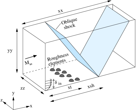
Figure 1: Schematic overview of the computational setup for the DNS cases.

A schematic view of the flow configuration investigated is shown in figure 1. The overall size of the computational domain is $L_{x}\times L_{y}\times L_{z}=120\delta_{in}\times 35\delta_{in}\times 10\delta_{in}$ in the streamwise (x), wall-normal (y) and spanwise (z) directions, respectively, $\delta_{in}$ being the thickness (based on 99 % of the external velocity) of the laminar boundary layer imposed at the inflow station. At the domain inlet, the Reynolds number based on the momentum thickness is $Re_{\theta}=6424$ and the freestream Mach number is $M_{\infty}=1.7$. A strip of roughness elements of width $4.5\delta_{in}$ is centered around a streamwise distance $x_{t}=31\delta_{in}$ from the domain inlet. Ten hemispherical elements of height $k=0.5\,\delta_{95}$ are randomly distributed along the entire spanwise width. Here, $\delta_{95}$ is the thickness (based on 95 % of the external velocity) of the boundary layer at the trip location. The Reynolds number at the trip is $Re_{x_{t}}=1.4\times 10^{6}$, which coincides with the experimental value considered by Giepman et al. (2016). The corresponding roughness Reynolds number, i.e. the Reynolds number associated with the element height $k$ and quantities evaluated at the roughness edge, is $Re_{k}=3.1\times 10^{3}$, a value sufficiently high to trigger roughness-induced transition (Tani, 1969; Bernardini et al., 2014).

We run a total of five DNS, whose parameters are listed in table 1. Case BL-TRIP corresponds to the simulation of a boundary layer tripped by roughness elements without any impinging shock. The other cases include shock/boundary-layer interactions for varying impingement location and shock strength. We choose two values of shock strength, corresponding to flow deviations $\phi=3^{o}$ and $\phi=6^{o}$. For a given shock strength, we choose two points of shock impingement, $x_{s}/\delta_{in}=48$ and $x_{s}/\delta_{in}=83.8$, corresponding to (see section III) a transitional- and a turbulent boundary layer, respectively. For two of the DNS cases (BL-TRIP and SH3-TU), experimental data from Giepman et al. (2016) are available for comparison.

Test case	$M_{\infty}$	$Re_{\theta}$	$\phi$	$x_{t}/\delta_{in}$	$x_{s}/\delta_{in}$	Grid	Interaction
BL-TRIP	1.7	6424	-	31	-	$4096\times 592\times 384$	No shock
SH3-TR	1.7	6424	3∘	31	48	$4096\times 592\times 384$	transitional
SH3-TU	1.7	6424	3∘	31	83.8	$4096\times 592\times 384$	turbulent
SH6-TR	1.7	6424	6∘	31	48	$4096\times 592\times 384$	transitional
SH6-TU	1.7	6424	6∘	31	83.8	$4096\times 592\times 384$	turbulent

Table 1: Details of the parameters for the DNS cases. $M_{\infty}$ is the freestream Mach number, $Re_{\theta}$ is the Reynolds number based on the momentum thickness at the inlet of the computational domain, and $\phi$ is the flow deflection angle. The distances from the leading edge to the roughness elements ($x_{t}$) and the shock impingement point ($x_{s}$) are also specified.

II.2 Numerical Method

We discretize the flow domain using a Cartesian grid and solve the three-dimensional compressible Navier-Stokes equations for a perfect gas with Fourier heat law and Newtonian viscous terms. The fluid under consideration is air with a value of specific heat ratio $\gamma=1.4$, specific gas constant $R=287$ $KJ/kg^{o}K$ and molecular Prandtl number $\mbox{{Pr}}=0.72$. We assume the molecular viscosity $\mu$ to depend on the temperature $T$ through the Sutherland’s law and compute the thermal conductivity as $k_{c}=c_{p}\mu/\mbox{{Pr}}$, where $c_{p}$ is the specific heat at constant pressure. We employ $4096\times 592\times 384$ points for discretization along the streamwise, wall-normal and spanwise directions, respectively, and generate a uniform grid spacing in the wall-parallel directions. In the wall-normal direction we cluster the grid nodes towards the wall by adopting a hyperbolic sine mapping ranging from $y=0$ up to $y=5\delta_{in}$, which is succeeded by a uniform mesh spacing using a suitable smoothing in the connecting zone. We ensure sufficient grid refinement by evaluating the wall units at $x/\delta_{in}=83.8$ (turbulent regime) for case BL-TRIP. The wall units are obtained by normalizing the grid spacing in terms of the viscous length scale $\delta_{v}$, and take the value of $\Delta x^{+}=4.63$ and $\Delta z^{+}=4.12$ along the streamwise and spanwise directions, respectively. Along the wall-normal direction, the value ranges from $\Delta y^{+}=1.02$ at the wall to $\Delta y^{+}=21.4$ at the edge of the boundary layer.

The boundary conditions are specified as follows. At the inlet, a laminar boundary layer is imposed, whose profile is determined from the solution of the generalized Blasius equations (White, 1974). An oblique shock wave is introduced at the top of the domain by locally enforcing the inviscid jump relations so as to mimic the effect of the shock generator. Non-reflecting boundary conditions are enforced at the top wall and at the outlet of the domain to avoid spurious wave reflections. A characteristic wave decomposition is also applied at the adiabatic no-slip wall to ensure perfect reflection of acoustic waves.

The governing equations are solved using an in-house finite-difference flow solver, widely validated for wall-bounded flows and SBLI in the transonic and supersonic regimes (Pirozzoli et al., 2010; Bernardini et al., 2016a). The solver is based on state-of-the-art numerical algorithms designed to tackle the challenging problems associated with high-speed turbulent flow solutions, allowing to accurately resolve a wide spectrum of turbulent scales and to capture steep gradients without unwanted numerical oscillations. We discretize the convective terms of the governing equations using a sixth-order central differencing scheme, and in the shock regions, identified through the Ducros sensor (Ducros et al., 1999), we use a fifth-order WENO scheme. To improve the numerical stability, the convective terms are arranged in skew-symmetric form (Reiss and Sesterhenn, 2014) and the triple split proposed by Kennedy and Gruber (2008) is applied in a locally conservative formulation. The viscous terms are expanded to Laplacian form and discretized using a sixth-order central differencing scheme, which guarantees physical dissipation at the smallest scales resolved by the computational mesh. The solution is advanced in time using a third-order, low-storage, explicit Runge-Kutta algorithm (Bernardini and Pirozzoli, 2009). The presence of the roughness elements is managed by means of the immersed-boundary (IB) method, that allows to deal with embedded geometries of arbitrary shape on a Cartesian grid. In the present study, the IB method is implemented following the approach proposed by de Tullio et al. (2007) for compressible flows. Additional details on the implementation can be found in Bernardini et al. (2016b).

We carry out the simulations using 2048 cores on the Lenovo NeXtScale platform at the Italian computing center CINECA, using a total budget of 2.25 Mio. CPU hours. The flow statistics were computed over a time period of about $327\delta_{in}/U_{\infty}$ using around 1200 flow fields. In the present work, we normalize the streamwise distance either using the trip location i.e. $x_{t}^{*}=(x-x_{t})/\delta_{95}$, or by the inviscid shock impingement point, i.e. $x_{s}^{*}=(x-x_{s})/\delta_{in}$.

III Boundary-layer transition

In this section, we look at the effect of the transition device on the incoming boundary layer in the absence of the impinging shock, and we provide a characterization of the boundary-layer evolution along the streamwise direction.

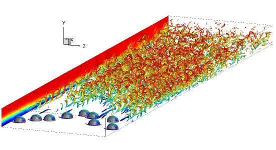
Figure 2: Three-dimensional visualization of vortical structures past the roughness elements for the case BL-TRIP obtained as isosurfaces of the swirling strength, colored by the mean streamwise velocity using sixty contour levels ranging from $-0.125\leq U/U_{\infty}\leq 1$.

The incoming laminar boundary layer is perturbed after encountering the roughness elements at $x_{t}^{*}=0$, and since the roughness height is above the critical value (Bernardini et al., 2012), transition to turbulence occurs further downstream. Figure 2, where isosurfaces of the swirling strength criterion are reported, shows the typical pattern to transition observed in previous studies of roughness-induced transition (Acarlar and Smith, 1987; Redford et al., 2010), with the formation and shedding of hairpin vortical structures past the roughness elements, which evolve in the streamwise direction leading to the flow breakdown. This behavior is associated to the instability of the detached shear layer on the top of roughness edge and has been observed across a wide range of Mach numbers (Bernardini et al., 2014).

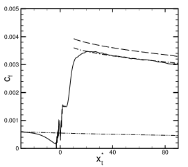
Figure 3: Distribution of the mean skin friction coefficient along the streamwise direction from DNS (solid line) for the case BL-TRIP. Also shown are the laminar $c_{f}$ values (dash dot dot) and the turbulent $c_{f}$ values from the Kármán-Schoenherr (dash dot; see Eq. (1)) and Blasius (dashed;see Eq. (2)) relations.

We report the distribution of the time- and spanwise-averaged skin friction coefficient $c_{f}=\tau_{w}/q_{\infty}$ along the streamwise direction in figure 3, $\tau_{w}$ and $q_{\infty}$ being the wall-shear stress and free-stream dynamic pressure, respectively. Upstream of the roughness elements, the skin friction is lower than the corresponding laminar solution, as a consequence of the perturbation induced by the tripping device. Beyond the roughness strip, $c_{f}$ increases rapidly to about seven times the corresponding laminar value and gradually decreases further, attaining values typical of a turbulent boundary layer. For reference purpose, we also include in the figure the $c_{f}$ predictions obtained from two theoretical expressions for turbulent flows, the incompressible skin-friction correlation of Kármán-Schoenherr,

$$c_{fi}=1/(17.08(\log_{10}Re_{\theta_{i}})^{2}+25.11\log_{10}Re_{\theta_{i}}+6.012),$$ (1)

and the Blasius correlation,

$$c_{fi}=0.026/Re_{\theta_{i}}^{1/4},$$ (2)

where the subscript ‘i’ refers to the incompressible regime. These relations are extended to compressible flows via the van Driest II transformation (for adiabatic wall) given by

$$c_{f_{i}}=F_{c}c_{f},\hskip 28.45274ptRe_{\theta_{i}}=F_{\theta}Re_{\theta},$$ (3)

where

$$F_{c}=\frac{T_{w}/T_{\infty}-1}{\arcsin^{2}\alpha},\hskip 28.45274ptF_{\theta}=\frac{\mu_{\infty}}{\mu_{w}},\hskip 28.45274pt\alpha=\frac{T_{w}/T_{\infty}-1}{\sqrt{T_{w}/T_{\infty}(T_{w}/T_{\infty}-1)}}.$$ (4)

We observe a good match between the $c_{f}$ distribution obtained from the DNS and the Kármán-Schoenherr prediction for $x_{t}^{*}>40$, whereas the Blasius expression overpredicts the DNS result by about ten percent.

Figure 4: Mean velocity profiles ($U/U_{e}$) along the wall-normal direction at various streamwise locations for the case BL-TRIP. Lines denote the DNS results and symbols represent the experimental data of Giepman et al. (2016).

A comparison of the DNS data with the experiments of Giepman et al. (2016) is reported in figure 4, where mean velocity profiles at various stations along the streamwise direction are shown. The first location ($x_{t}^{*}=-25$) corresponds to the region upstream of the tripping elements, and the velocity profile is characterized by an extended linear behavior typical of a laminar boundary layer. A strongly perturbed profile is observed at $x_{t}^{*}=0$, with the presence of two inflection points, which indicates the onset of the instabilities due to the flow interaction with the tripping elements. As a consequence of the transition process, the mean velocity profiles at subsequent stations ($x_{t}^{*}=25$ and $x_{t}^{*}=50$) become fuller, with a steeper velocity gradient at the wall. We obtain a very good agreement with the experimental data, which demonstrates the capability of the simulation in accurately predicting the streamwise evolution of the flow and capturing the length-scale of the transition process.

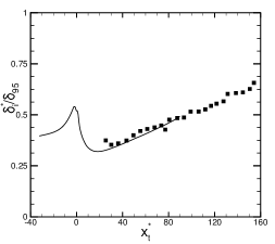
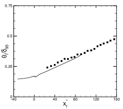
a)    b) c)

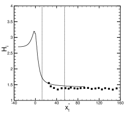
Figure 5: Distribution of the incompressible (a) displacement thickness, (b) momentum thickness and (c) shape factor for the case BL-TRIP. Lines denote the DNS results and symbols represent the experimental data of Giepman et al. (2016). The two vertical dotted lines reported in panel (c) denote the location of shock impingment for the SBLI flow cases discussed in the later sections.

A further comparison between the DNS and the experiment is provided in figure 5, where the evolution of the boundary layer is described in terms of incompressible displacement thickness ($\delta^{*}_{i}$), momentum thickness ($\theta_{i}$) and shape factor ($H_{i}$),

$$\delta^{*}_{i}=\int_{0}^{\delta_{e}}\left(1-\frac{U}{U_{e}}\right)\mathrm{d}y,\qquad\theta_{i}=\int_{0}^{\delta_{e}}\frac{U}{U_{e}}\left(1-\frac{U}{U_{e}}\right)\mathrm{d}y,\qquad H_{i}=\frac{\delta_{i}^{*}}{\theta_{i}}.$$ (5)

The agreement between the DNS results and the experimental data is very satisfactory, also considering the challenges of performing PIV measurements in extremely thin transitional boundary layers with non-uniform seeding distributions. Past the tripping elements the displacement thickness initially decreases as a consequence of the transition process that fills-up the velocity profile, it achieves a minimum at $x^{*}_{t}\approx 15$ and then it starts to rise. On the other hand the momentum thickness is characterized by a steady growth and its post-trip value is always larger than the value computed at the trip location. The distribution of the shape factor reflects the transition process undergone by the boundary layer. It has an initial value of about 2.7, typical of a laminar boundary layer and attains a peak of about 3.2 at the roughness location. Past the interaction, the shape factor displays a drastic drop to about 1.4, which is a value typical of a turbulent boundary layer (Smits and Dussauge, 2006), achieved approximately for $x_{t}^{*}>40$.

IV Effect of impinging shock

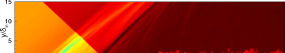
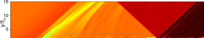
a) b) c) d)

Figure 6: Contours of instantaneous density for the four cases of shock impingement, a) SHK3-TR, b) SH3-TU, c) SH6-TR and d) SH6-TU. Fifty contour levels are shown in the range of $0.56<\rho/\rho_{\infty}<1.33$ for the $\phi=3^{o}$ cases and $0.56<\rho/\rho_{\infty}<1.83$ for the $\phi=6^{o}$ cases.

In this section we investigate the interaction of an impinging shock with the spatially evolving boundary layer discussed in the previous section, with the main aim of characterizing the effect of the incoming boundary-layer state (transitional or turbulent) on the properties of the interaction. To that purpose, we analyze the results of the four DNS listed in table 1, performed for two values of shock strength ($\phi=3^{o}$ and $\phi=6^{o}$) and two shock impingement locations $x_{s}/\delta_{in}=48$ and $83.8$ ($x_{t}^{*}=17.7$ and $55$), corresponding to transitional and turbulent SBLI, respectively. This classification is supported by the results discussed in the previous section (see in particular figure 5c).

To provide a qualitative overview of the flow organization, we report in figure 6 contours of the instantaneous density in a longitudinal $x-y$ plane. The density field highlights very well the wave system originated as a consequence of the interaction process, mainly consisting of the impinging and the reflected shock, as well as a series of waves (compression-expansion-compression) radiating in the freestream, arising from the perturbation of the boundary layer induced by the tripping device. We point out that the other feature typically observed in a strong SBLI involving a separation bubble, a fan of expansion waves associated with the reattachment of the boundary layer, is not observed in figure 6 and both the transitional and turbulent interaction cases share the same qualitative behavior. This reveals that the present interactions do not involve a massive separation of the flow, contrary to the case of an untripped laminar oblique shock-wave reflection at $\phi=3^{\circ}$, considered under the same flow conditions (Mach- and Reynolds numbers) in the experimental work by Giepman et al. (2015), who highlighted the presence of a large separation bubble. A major role is played by the strength of the impinging shock, which determines the extent of the interaction zone, that significantly increases with the deflection angle $\phi$.

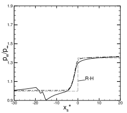
a)    b)

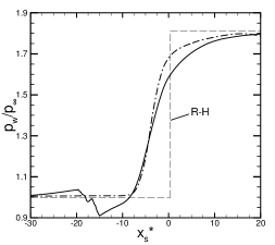
Figure 7: Streamwise distribution of mean wall pressure for (a) $\phi=3^{o}$ and (b) $\phi=6^{o}$. Solid lines refer to transitional interactions and dash-dot lines denote turbulent interactions. $R-H$ denotes the inviscid distribution resulting from the Rankine-Hugoniot jump conditions (dashed).

The distribution of the mean wall pressure is shown in figure 7, together with the inviscid pressure jumps predicted by the Rankine-Hugoniot relations. In all cases, the wall pressure exhibits a sharp rise upstream of the nominal shock impingement point, followed by a slower increase further downstream, which is more gradual in the case of the transitional SBLI. On the other hand, we observe that the beginning of the interaction is rather independent of the nature of the incoming boundary layer (transitional or turbulent), and the extent of the upstream influence region is determined by the shock strength.

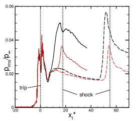
Figure 8: The streamwise variation of the rms wall pressure for the $\phi=3^{o}$ (red) and the $\phi=6^{o}$ (black) cases with the transitional (solid) and turbulent (dashed) interactions.

Figure 8 shows the root-mean-square of wall pressure fluctuations ($p_{w_{rms}}$) for all shock-impingement cases. The $p_{w_{rms}}$ rise across the interaction region is sligthly higher for the turbulent interactions as compared to the corresponding transitional cases, for both the incident shock angles. The post-shock decay for the two types of interaction also varies, with the turbulent cases displaying a steeper decline past the interaction region compared to the corresponding transitional case. The transitional interactions have a broader post-shock decay region, with the $\phi=6^{\circ}$ case also displaying a local minimum at the nominal shock impingement point.

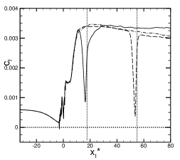
a)    b)

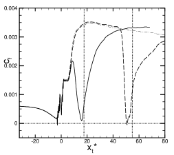
Figure 9: Distribution of skin friction coefficient along the streamwise direction for the shock impingement cases at (a) $\phi=3^{o}$ and (b) $\phi=6^{o}$. Solid lines refer to the transitional interactions and dashed lines denote the turbulent interactions. The skin friction coefficient for the case without shock impingement is also shown (dash-dot). The vertical dotted lines the nominal shock impingment location.

The effectiveness of boundary-layer tripping in suppressing a shock-induced separation can be identified by the distribution of the skin friction coefficient $c_{f}$, displayed in Fig 9 for all the shock impingement cases. In the interaction region the wall shear stress is characterized by a remarkable drop, associated with the lift off of the boundary layer, followed by a gradual recovery. The $c_{f}$ curves show that in all the cases, even those at higher shock strength, mean separation is not observed, and tripping the boundary layer eliminates the large separation bubble found in a laminar interaction. This quantitatively confirms our expectations drawn from the inspection of figure 6. The skin friction levels remain well above the zero line for the cases SH3-TR and SH3-TU, whereas they are almost tangent for the cases SH6-TR and SH6-TU, which can be classified as cases with incipient separation. Quite surprisingly, the minimum value of the skin friction is lower in the turbulent interaction than in the transitional cases, although the width of the region where the $c_{f}$ value drops due to the shock impingement is wider in the transitional interactions.

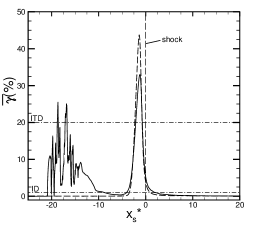
a)    b)

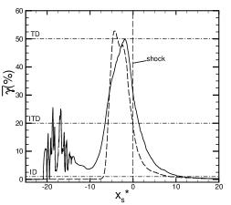
Figure 10: Distribution of statistical probability of wall points along the streamwise direction with $\partial u/\partial y<0$ for (a) $\phi=3^{o}$ and (b) $\phi=6^{o}$, for the transitional interaction cases (solid lines) and the turbulent interaction cases (dashed lines). The horizontal lines denote the incipient detachment (ID), intermittent transitory detachment (ITD) and the transitory detachment (TD) levels.

The absence of a mean separation clearly does not preclude the possibility of instantaneous zones with locally reversed flow. We characterize the regions of instantaneous separation by plotting the statistical probability ($\overline{\gamma}$) of the the wall points with negative $\partial u/\partial y$, where $u$ is the instantaneous streamwise velocity. Simpson (1989) classified the boundary-layer detachment based on how frequently the backflow occurs. A statistical probability of backflow of 1% of the total sampling is denoted as incipient detachment (ID), while that amounting to 20 % is classified as intermittent transitory detachment (ITD). A 50 % probability of backflow is termed as transitory detachment (TD), which clearly indicates a separation in the mean.

Figure 10a shows the statistical probability of instantaneous separation for the interactions at $\phi=3^{o}$. In the region of shock impingement ($x_{s}^{*}=0$), both the flow cases (SH3-TR and SH3-TU) exceed the ITD level, and the peak probability of separation for the turbulent interaction is slightly higher than that of the transitional interaction. The same plot for the flow cases at higher angle of incidence $\phi=6^{o}$ is shown in figure 10b. As expected, we observe higher levels of instantaneous separation in comparison to the lower incidence cases, with the turbulent interaction exceeding the transitory detachment level. In the transitional interaction case, although the peak percentage of separation is not as high, the width of the separation region exceeds that of the turbulent interaction zone by about 36 % at the ITD level.

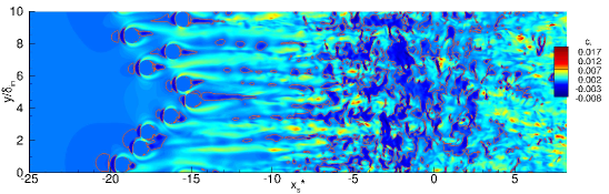
a) b)

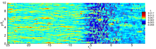
Figure 11: Contours of instantaneous skin friction for the flow cases (a) SH6-TR and (b) SH6-TU. The iso-line $c_{f}=0$ is denoted in orange.

The instantaneous flow separation can be clearly visualized by plotting the wall skin friction contour, as carried out for the $\phi=6^{o}$ shock impingement cases in figure 11. The isolines correspond to zero skin friction level indicating areas of reverse flow. In agreement with the statistical probability of instantaneous separation discussed previously, the region of separation is slightly wider in the transitional interaction case as compared to the turbulent one.

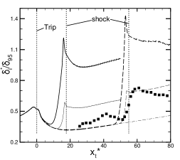
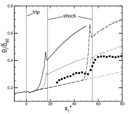
a)    b) c)

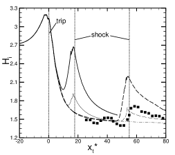
Figure 12: Distribution of the incompressible (a) displacement thickness, (b) momentum thickness and (c) shape factor for all the shock impingement cases. Lines denote DNS results. Symbols refer to experiments of Giepman et al. (2016).

The development of the boundary layer across the interaction is described in figure 12, where we provide distributions of the incompressible displacement thickness, momentum thickness and shape factor. As a reference, we also plot in the figure the DNS results for the transitional boundary layer without any shock and the experimental data corresponding to the flow case SH3-TU. For all the interactions, the boundary-layer thicknesses show a rapid increase in the region of shock impingement, which is remarkably higher for the flow cases at $\phi=6^{o}$ angle of incidence. While the shock strength plays an important role, the boundary-layer growth does not seem greatly affected by the state of the incoming boundary layer, the jump of the momentum and displacement thickness being approximately the same for the corresponding interactions. For the SH3-TU case, the agreement with the experimental data is fair, especially for the prediction of the location and amplitude of the jump of $\delta_{i}$ and $\theta_{i}$. The discrepancies observed upstream of the interaction, where the experiments exhibit a spurious peak, can be attributed to the aero-optical distortion in the measurement and does not reflect the actual flow field (Giepman et al., 2016). The distributions of $H_{i}$ match quite well and highlight the boundary-layer distortion in the interaction region, with the velocity profile becoming emptier due to the effect of the adverse pressure gradient, leading to higher values of the shape factor.

Test case	$M_{\infty}$	$\phi$	$\beta$	Interaction	$\delta^{*}/\delta_{in}$	$L/\delta_{in}$	$L^{*}$	$Re_{\theta}$	$\overline{k}$	$P_{3}/P_{1}$	$S_{e}^{*}$	Inference
SH3-TR	1.7	3	38.9	transitional	0.32	3.2	0.56	8150	3	1.35	0.51	attached
SH3-TU	1.7	3	38.9	turbulent	0.36	3.5	0.55	12450	2.5	1.35	0.44	attached
SH6-TR	1.7	6	42.1	transitional	0.41	6.1	1.74	7240	3	1.81	1.11	insipient Sep.
SH6-TU	1.7	6	42.1	turbulent	0.35	6.1	2.04	12140	2.5	1.81	1.02	insipient Sep.

Table 2: Scaling analysis of transitional and turbulent SBLI. $L^{*}$ is the dimensionless value of the interaction length scale, $\beta$ is the shock angle and $S_{e}^{*}$ the separation criterion proposed by Souverein et al. (2013).

We now look at some of the characteristics of the interaction in the transitional and turbulent regime at varying shock angles. An important defining parameter for any SBLI is the characteristic interaction length $L$, which is defined as the distance between the wall-extrapolated point of the reflected shock and the nominal impinging shock location.

Based on a mass-balance analysis, Souverein et al. (2013) proposed a non-dimensional form of the interaction length scale applicable for turbulent SBLI with adiabatic wall boundary conditions (both, oblique shock impingement and compression corner),

$$L^{*}=\frac{L}{\delta_{in}^{*}}G_{3},$$ (6)

where $G_{3}$ is $\sin(\beta)\sin(\phi)/\sin(\beta-\phi)$, $\beta$ is the shock angle. This new dimensionless interaction length also classifies the interactions as attached, incipiently separated or fully separated, based on its value. While a value of $L^{*}\downarrow 1$ corresponds to an attached flow, the cases with incipient separation have $1<L^{*}<2$, and the separated interactions have $L^{*}$ values larger than two.

We provide the values of $L^{*}$ for our cases with shock impingement in table 2. For the two cases at $\phi=3^{o}$ (SH3-TR and SH3-TU), the values of $L^{*}$ are less than unity, and correspond to attached flow, as shown by the skin-friction results presented in figure 9a. For the cases at $\phi=6^{o}$, $L^{*}=1.74$ associated with the transitional interaction (SH6-TR) correctly classifies it as an incipient separation case. The borderline value $L^{*}=2.04$ associated with the flow case SH6-TU, while strictly classifies it as a separated interaction, is indicative of of an incipient separation as displayed by figure 9b.

Souverein et al. (2013) also proposed an additional parameter to characterize the SBLI in terms of the ratio in the pressures before ($P_{1}$) and after ($P_{3}$) the shock system. This non-dimensional parameter is given by

$$S_{e}^{*}=\frac{2\overline{k}}{\gamma}\frac{\frac{P_{3}}{P_{1}}-1}{M_{\infty}^{2}},$$ (7)

and can be written as a function of free-stream Mach number $M_{\infty}$, flow deflection angle $\phi$ and specific heat ratio $\gamma$. The constant $\overline{k}$ as observed from the experimental data can either take a value of about 3 for $Re_{\theta}\leq 1\times 10^{4}$ or a value of about 2.5 for $Re_{\theta}>1\times 10^{4}$, where $Re_{\theta}$ is the Reynolds number based on the momentum thickness upstream of the interaction. The values of $Re_{\theta}$, and the associated values of $\overline{k}$ for each of the cases are listed in table 2.

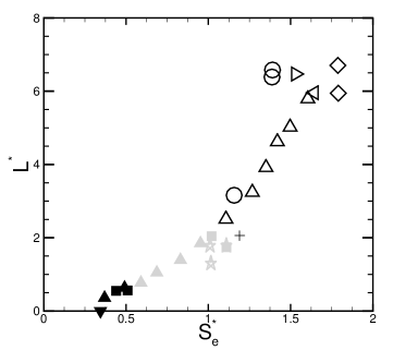
Figure 13: Scaling of the interaction length. Separation criterion $S_{e}^{*}$ plotted against the interaction length $L^{*}$ for the DNS flow cases (squares) compared with the available experimental data. Refer to Souverein et al. (2013) for the interpretation of symbols.

According to the classification of Souverein et al. (2013), a value of $S_{e}^{*}<1$ corresponds to attached interactions and $S_{e}^{*}>1$ represents interactions with boundary-layer separation. The values of $S_{e}^{*}$ for each of our cases is given in table 2. Souverein et al. (2013) suggested that the interaction length $L^{*}$ plotted in combination with the separation criterion $S_{e}^{*}$ would collapse the data along a single trend line irrespective of Reynolds number, Mach number and interaction type (oblique shock impingement and compression corner). This scaling is tested for our flow cases in figure 13, where DNS data are reported with available experiments, and colors are used to identify attached (black), incipiently separated (grey) or separated (white) interactions. We observe that, for all flow cases, our DNS data follow the experimental trend and fall within the acceptable range of scatter, suggesting that the scaling analysis proposed by Souverein et al. (2013) for turbulent SBLI, could be equally applied to describe transitional interactions.

V Conclusions

We have performed a series of direct numerical simulations to investigate the effect of an oblique shock wave impinging on transitional and turbulent boundary layers at $M_{\infty}=1.7$, with the main aim of evaluating the effectiveness of a transitional boundary layer to suppress shock-induced separation.

The incoming laminar boundary layer was tripped by a strip of distributed roughness elements, which enabled a rapid transition to turbulence. A single DNS carried out without the presence of any impinging shock wave helped to characterize the boundary-layer transition region and to validate the numerical approach by means of a favorable comparison with available experimental data in terms of mean velocity profiles, boundary layer thicknesses and shape factor.

Four DNS cases were considered in the present study based on varying shock impingement locations along the streamwise distance (corresponding to transitional or turbulent interactions), and also based on varying shock strength (flow deflection angles $\phi=3^{o}$ and $\phi=6^{o}$). We observed a clear suppression of shock-induced mean separation in both the transitional and turbulent interaction cases, inferred by the distribution of the skin friction coefficient. This observation applies to both the weak as well as the strong interaction cases considered in our study. A higher peak in the probability of the instantaneous separation was observed for the turbulent interactions, although the transitional cases exhibited wider regions of instantaneous separation.

The scaling analysis for the interaction length proposed by Souverein et al. (2013) for turbulent shock/boundary-layer interactions was tested for all the flow cases considered here and it was found to be applicable for our DNS, including the transitional interactions. Furthermore, the separation criterion $S^{*}_{e}$, only dependent on the Mach number and flow deflection angle, correctly classified the present interactions as attached or close to incipient separation.

Overall, our results provide numerical evidence that a transitional interaction retains the beneficial features of a turbulent interaction in terms of suppression of mean separation. Therefore, for practical SBLI applications, it seems to be reasonable to trip the boundary layer a short distance upstream of the impinging shock to remove the separation bubble, maximizing the region with a low skin friction coefficient. Obviously, such encouraging considerations are based on a DNS database of limited extent and further investigations are needed to completely characterize transitional SBLI. Future efforts will be devoted to include the effects of different tripping devices, as well as to expand the range of investigated Mach- and Reynolds numbers.

References

References

- Giepman et al. [2016] R. H. M. Giepman, R. Louman, F. F. J. Schrijer, and B. W. van Oudheusden. Experimental study into the effects of forced transition on a shock-wave/boundary-layer interaction. AIAA Journal, 54(4):1313–1325, 2016.
- Souverein et al. [2013] L. J. Souverein, P.G. Bakker, and P. Dupont. A scaling analysis for turbulent shock-wave/boundary-layer interactions. Journal of Fluid Mechanics, 714:505–535, 2013.
- Dolling [2001] D. S. Dolling. Fifty years of shock-wave/boundary layer interaction research: what next? AIAA J, 39:1517–1531, 2001.
- Dupont et al. [2006] P. Dupont, C. Haddad, and J.F. Debiève. Space and time organization in a shock-induced separated boundary layer. J. Fluid Mech., 559:255–277, 2006.
- Touber and Sandham [2009] E. Touber and N. D. Sandham. Large-eddy simulation of low-frequency unsteadiness in a turbulent shock-induced separation bubble. Theoretical and Computational Fluid Dynamics, 23:79–107, 2009.
- Souverein et al. [2010] L. Souverein, P. Dupont, J. F. Debiève, J. P. Dussauge, B. W. van Oudheusden, and F. Scarano. Effect of interaction strength on unsteadiness in turbulent shock-wave-induced separations. AIAA J., 48:1480–1493, 2010.
- Clemens and Narayanaswamy [2014] N.T. Clemens and V. Narayanaswamy. Low-frequency unsteadiness of shock wave/turbulent boundary layer interactions. Annu. Rev. Fluid Mech., 46:469–492, 2014.
- Adamson and Messiter [1980] T. C. Adamson and A. F. Messiter. Analysis of two-dimensional interactions between shock waves and boundary layers. Annu. Rev. Fluid Mech., 12:103–138, 1980.
- Delery [1985] J.M. Delery. Shock wave/turbulent boundary layer interaction and its control. Prog. Aerosp. Sci., 22:209–280, 1985.
- Babinsky et al. [2009] H Babinsky, Yl Li, and CW Pitt Ford. Microramp control of supersonic oblique shock-wave/boundary-layer interactions. AIAA journal, 47(3):668, 2009.
- Hakkinen et al. [1959] R. J. Hakkinen, I. Greber, L. Trilling, and S. S. Abarbanel. The interaction of an oblique shock wave with a laminar boundary layer. Technical Report 2-18-59W, NASA MEMO, 1959.
- Giepman et al. [2015] R. H. M. Giepman, F. F. J. Schrijer, and B.W. van Oudheusden. High-resolution piv measurements of a transitional shock wave–boundary layer interaction. Experiments in Fluids, 56(6):113, 2015.
- Degrez et al. [1987] G. Degrez, C. H. Boccadoro, and J. F. Wendt. The interaction of an oblique shock wave with a laminar boundary layer revisited. An experimental and numerical study. J. Fluid Mech., 177:247–263, 1987.
- Katzer [1989] E. Katzer. On the lengthscales of laminar shock/boundary-layer interaction. J. Fluid Mech., 206:477–496, 1989.
- Yao et al. [2007] Y. Yao, L. Krishnan, N. Sandham, and G. T. Roberts. The effect of Mach number on unstable disturbances in shock/boundary-layer interactions. Physics of Fluids, 19(5):054104, 2007.
- Gadd [1957] G. E. Gadd. A theoretical investigation of laminar separation in supersonic flow. Journal of the Aeronautical Sciences, 24(10):759–771, 1957.
- Chapman et al. [1957] D. R. Chapman, D. M. Kuehn, and H. K. Larson. Investigation of separated flow in supersonic and subsonic streams with emphasys on the effect of transition. Technical Report 3869, NACA TN, 1957.
- Greene [1970] J. E. Greene. Interactions between shock waves and turbulent boundary layers. Progress in Aerospace Science, 11:235–340, 1970.
- Stollery [1975] J. L. Stollery. Laminar and turbulent boundary layer separation at supersonic and hypersonic speeds. Technical report, AGARD, 1975.
- Delery and Marvin [1986] J. Delery and J. Marvin. Shock wave boundary layer interactions. Technical Report 280, AGARDograph, 1986.
- Gai [1977] S. L. Gai. Shock-wave/boundary-layer interaction with suction. Z. Flugwiss. Weltraumforsch, 1(2):97–101, 1977.
- Krogmann et al. [1985] P. Krogmann, E. Stansewsky, and P. Thiede. Effects of suction on shock/boundary-layer interaction and shock-induced separation. J. Aircr., 22(1):37–42, 1985.
- Holden and Babinsky [2005] H. A. Holden and H. Babinsky. Separated shock-boundary-layer interaction control using streamwise slots. J. Aircr., 42(1):166–171, 2005.
- Smith et al. [2004] A. Smith, H. Babinsky, J. L. Fulker, and P. R. Ashill. Shock-wave/boundary-layer interaction control using streamwise slots in transonic flows. J. Aircr., 41(3):540–546, 2004.
- Raghunathan and Mabey [1987] S. Raghunathan and D. G. Mabey. Passive shock-wave/boundary-layer control on a wall-mounted model. AIAA J., 25(2):275–278, 1987.
- Mccormick [1993] D. C. Mccormick. Shock/boundary-layer interaction control with vortex generators and passive cavity. AIAA J., 31(1):91–96, 1993.
- Anderson et al. [2006] B. H. Anderson, J. Tinapple, and L. Surber. Optimal control of shock-wave/turbulent boundary-layer interactions using micro-array actuation. In 3rd AIAA Flow Control Conference, San Francisco, California, 5-8 June, 2006.
- Sandham et al. [2014] N.D. Sandham, E. Schülein, A. Wagner, S. Willems, and J. Steelant. Transitional shock-wave/boundary-layer interactions in hypersonic flow. Journal of Fluid Mechanics, 752:349–382, 2014.
- Davidson and Babinsky [2014] T. S. Davidson and H. Babinsky. An investigation of interactions between normal shocks and transitional boundary layers. 44th AIAA Fluid Dynamics Conference, Atlanta, GA, 3334, 2014.
- Davidson and Babinsky [2015] T. S. Davidson and H. Babinsky. Transition location effects on normal shock wave/boundary layer interactions. 53rd AIAA Aerospace Sciences Meeting, Kissimmee, Florida, 1975, 2015.
- Tani [1969] I. Tani. Boundary-layer transition. Annual Review of Fluid Mechanics, 1(1):169–196, 1969.
- Bernardini et al. [2014] M. Bernardini, S. Pirozzoli, P. Orlandi, and S. K. Lele. Parameterization of boundary-layer transition induced by isolated roughness elements. AIAA Journal, 52(10):2261–2269, 2014.
- White [1974] F. M. White. In Viscous Fluid Flow. McGraw-Hill, New York, 1974.
- Pirozzoli et al. [2010] S. Pirozzoli, M. Bernardini, and F. Grasso. Direct numerical simulation of transonic shock/boundary layer interaction under conditions of incipient separation. Journal of Fluid Mechanics, 657:361–393, 2010.
- Bernardini et al. [2016a] M. Bernardini, I. Asproulias, J. Larsson, S. Pirozzoli, and F. Grasso. Heat transfer and wall temperature effects in shock wave turbulent boundary layer interactions. Phys. Rev. Fluids, 1:084403, 2016a.
- Ducros et al. [1999] F. Ducros, V. Ferrand, F. Nicoud, D. Darracq, C. Gacherieu, and T. Poinsot. Large-eddy simulation of the shock/turbulence interaction. J. Comput. Phys., 152(2):517–549, 1999.
- Reiss and Sesterhenn [2014] Julius Reiss and Jörn Sesterhenn. A conservative, skew-symmetric finite difference scheme for the compressible navier–stokes equations. Computers & Fluids, 101:208–219, 2014.
- Kennedy and Gruber [2008] C. A. Kennedy and A. Gruber. Reduced aliasing formulations of the convective terms within the navier-stokes equations. J. Comput. Phys., 227:1676, 2008.
- Bernardini and Pirozzoli [2009] M. Bernardini and S. Pirozzoli. A general strategy for the optimization of runge-kutta schemes for wave propagation phenomena. J. Comput. Phys., 228:4182, 2009.
- de Tullio et al. [2007] M.D. de Tullio, P. De Palma, G. Iaccarino, G. Pascazio, and M. Napolitano. An immersed boundary method for compressible flows using local grid refinement. J. Comput. Phys., 225(2):2098–2117, 2007.
- Bernardini et al. [2016b] Matteo Bernardini, Davide Modesti, and Sergio Pirozzoli. On the suitability of the immersed boundary method for the simulation of high-reynolds-number separated turbulent flows. Computers & Fluids, 130:84–93, 2016b.
- Bernardini et al. [2012] M. Bernardini, S. Pirozzoli, and P. Orlandi. Compressibility effects on roughness-induced boundary layer transition. International Journal of Heat and Fluid Flow, 35:45 – 51, 2012.
- Acarlar and Smith [1987] M.S. Acarlar and C. R. Smith. A study of hairpin vortices in a laminar boundary layer. part 1. hairpin vortices generated by a hemisphere protuberance. Journal of Fluid Mechanics, 175:1–41, 1987.
- Redford et al. [2010] J. A. Redford, N. D. Sandham, and G. T. Roberts. Compressibility effects on boundary-layer transition induced by an isolated roughness element. AIAA Journal, 48(12):2818 – 2830, 2010.
- Smits and Dussauge [2006] A. J. Smits and J. Dussauge. In Turbulent Shear Layers in Supersonic Flow. Springer-Verlag New York, 2006.
- Simpson [1989] R. L. Simpson. Turbulent boundary-layer separation. Annual Review of Fluid Mechanics, 21(1):205–232, 1989.