Modelling astronomical adaptive optics performance with temporally-filtered Wiener reconstruction of slope data
Abstract
We build on a long-standing tradition in Astronomical Adaptive Optics (AO) of specifying performance metrics and error budgets using linear systems modeling in the spatial-frequency domain.
Our goal is to provide a comprehensive tool for the calculation of error budgets in terms of residual temporally-filtered phase power-spectral-densities (PSDs) and variances. In addition, the fast simulation of AO-corrected PSFs provided by this method can be used as inputs for simulations of science observations with next-generation instruments and telescopes, in particular to predict post-coronagraphic constrast improvement for planet finder systems.
We extend the previous results presented in Correia et al correia14a to the closed-loop case with predictive controllers and generalise the analytical modelling of Rigaut et al rigaut98 , Flicker et al flicker07a and Jolissaint jolissaint10 . We follow closely the developments of Ellerbroek ellerbroek05 and propose the synthesis of a distributed Kalman filter to mitigate both aniso-servo-lag and aliasing errors whilst minimizing the overall residual variance. We discuss applications to (i) Analytic AO-corrected point-spread-function (PSF) modelling in the spatial-frequency domain; (ii) Post-coronagraphic contrast enhancement; (iii) Filter optimisation for real-time wave-front reconstruction; and (iv) PSF reconstruction from system telemetry.
Under perfect knowledge of wind-velocities we show that 60 nm rms error reduction can be achieved with the distributed Kalman Filter embodying anti-aliasing reconstructors on 10 m-class high-order AO systems, leading to contrast improvement factors of up to three orders of magnitude at few separations () for a 0-magnitude star and reaching close to 1 order of magnitude for a 12-magnitude star.
pacs:
(000.0000) General.I Introduction
Synthetic modelling of Adaptive Optics (AO) systems has been pursued over the years using linear approximations. These approximations allow a fast and accurate estimation of performance over a broad parameter range for both classical (single-conjugate) AO rigaut98 ; flicker07a ; jolissaint10 and multi-conjugate AO rigaut00 ; gavel04 ; ellerbroek05 . This is particularly relevant in the era of Extremely Large Telescopes (ELTs), where a high number of degrees of freedom incur high computational costs in full end-to-end simulations and likewise in real-time during on-sky observations.
In Correia et al correia14a post-facto spatial anti-aliasing filters were investigated. Here we generalize these results to the dynamic, temporally-filtered case, in particular for regular closed-loop operation. The temporal filtering of the loop is factored in by invoking, as elsewhere in the literature, the frozen-flow hypothesis, for which there is growing evidenceono16 ; poyneer09 .
A general state-space framework is employed to synthesise the closed-loop linear filters – a specific case being the commonly-used integrator controller – borrowing from the motivation and further developing the results of poyneer07 ; massioni11 on distributed filters. The latter relies on the hypothesis of phase spatial invariance. As such, the AO loop operations can all be approximated by convolutions with localised kernels which translate into filtering functions when a basis of complex exponentials is chosen. All parameters being equal, the two approaches above are equivalent but differ in how the controller is applied to the measurements. In direct space the data is convolved (after inverse Fourier-transforming the matrix of gains). In Fourier space, the Fourier transform of the wave-front measurements is taken, then each mode is weighted by a complex function (the filtering process) followed by an inverse Fourier transform to gather the reconstructed phase.
Although this is not a review paper we strive to generalise and provide further insight into previous work in this field. Our developments make extensive use of Fourier transforms, in both time and space over continuous and discrete supports (with the necessary adaptations), and the well-established relationships between the Laplace transform and Z-transforms oppenheim97 ; oppenheim99 .
The foreseeable applications of these results include
-
•
Analytic AO-corrected PSF modelling
-
•
Post-coronagraphic contrast enhancement
-
•
Filter optimisation for real-time wave-front reconstruction
-
•
Evaluation of error terms for post-processing system telemetry to reconstruct the AO-corrected PSF
Of particular interest for the analysis carried out here are cases where the use of an optical spatial filter poyneer04a is limited, such as in cases where the size of the sub-apertures compared to the turbulence coherent length makes it hard to reach a suitable trade-off between aliasing rejection (small spatial filter width) and robustness to changing seeing conditions (large spatial filter width) sauvage16 . In such cases a reconstruction process which can compensate for predicted aliasing errors is highly desirable, particularly in the case of high contrast imaging.
The formulation of the distributed Kalman filter (DKF) is motivated by physical and technological constraints. On the one hand complex-exponential (Fourier) modes are considered statistically independent (both spatially and temporally). On the other hand, if is the number of degrees of freedom, the runtime computation of modal coefficients can be accomplished using transforms that scale with , compared to operations required by standard linear-systems solvers (explicit vector-matrix multiplication). Thus such an approach has the potential to provide a much welcome improvement in runtime application. Moreover, since a distributed controller is obtained, the off-line computation of gains boils down to solving scalar (or small scale) algebraic equations in parallel for each Fourier mode.
Considering that Kalman filters are seamlessly obtained as the minimisers of the residual phase variance criterion (which is to say Strehl-ratio maximisers) they naturally achieve the best trade-off between aniso-servo-lag, spatial aliasing and propagated noise. Mitigation of these errors is crucial for achieving high post-coronagraphic contrast levels sufficiently close to the PSF core to enable the detection of Earth-mass companions orbiting nearby stars guyon05 .
Illustrative examples are given for two scenarios
-
1.
PSF modelling and performance optimisation for current general-purpose AO systems
-
2.
Post-coronagraphic raw constrast improvement in current 10m-class telescopes
using a distributed Kalman filter massioni11 ; poyneer08a with embedded temporal prediction of the atmosphere.
This paper is organised in the following way: Section II formulates the residual wave-front error statistics in the static and dynamic cases; Sec. III provides the distributed Kalman Filter formulation and reviews that of the integrator as a specific case covered by state-space models; Sec. IV outlines the modelling for Shack-Hartmann based AO; Sec.V and Sec. VI quantifies AO performance and raw contrast improvement when using optimal, time-predicive controllers; a summary is provided in Sec. VII.
II Residual wave-front error in the spatial-frequency domain
The errors present in an adaptive optics system can be separated into different categories according to their origin. Depending on the nature of the error they may be static or impacted by the AO loop. The specific errors considered in this paper are:
-
1.
Fitting error for modes beyond the AO correction region, i.e. spatial frequencies above , where is the deformable mirror pitch.
-
2.
Measurement noise due to photon and detector read noise.
-
3.
Aliasing due to spurious high-order frequencies which fold into the measurement during the discretisation process. correia14a .
-
4.
Aniso-servo-lag errors due to system delays and the angular separation between guide-stars and science objects.
We consider two cases – static and dynamic, i.e., with and without temporal filtering by an AO loop, in both open- and closed-loop mode.
The telescope aperture, which would break spatial stationarity is approximated by the general filtering functions for piston-removal correia14a ; ellerbroek05 . Therefore the final result is compatible with expressions in the spatial frequency domain using modal decompositions onto functions defined over an infinite plane. Tilde symbols are used to represent complex-valued variables in the spatial-frequency domain, each of which represent coefficients of harmonic functions whose relationship to spatial domain variables are given by standard Fourier transforms oppenheim97 .
II.1 Limiting static case: open-loop, ,
We start by providing suitable formulations for evaluating the individual AO error contributions in the highly idealised static case where any temporal aspects are momentarily set aside. This case is rather instructive as the limiting case when the WFS integration time is zero () and the delays are set to null () leading to simplifications when computing the instantaneous AO residual. Moreover, no time-dependence is associated to the wave-front sensor , spatial reconstruction and deformable mirror filtering functions. Spatial filters are indexed by the spatial frequency variable .
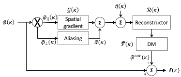
Figure 1 provides the general-case AO scenario in open-loop operation. Variables therein will be used throughout this document.
The (spatial) error functions, are described by the following relations
| (1) |
where represents the AO controllable region and its complement for a DM with regular actuator pitch matching the SH-WFS sub-aperture widths. refers to wave-fronts in the spatial-frequency domain. The upper-script represents the corrective phase applied by the DM. Note that in general but we include this term as the shape of the DM actuator functions can extend the controllable region beyond the limits stated above ellerbroek05 ; correia14a . In the following we drop the symbol when implicit and use interchangeably the notation for the power-spectral density (PSD) .
Let the piston-removed residual phase PSD be such that
| (2) |
in which is a Bessel function of the first kind. is the piston-removal filter within square brackets in Eq. (2) for a circular pupil of diameter .
Using the Parseval theorem, the residual (piston-removed) phase variance is defined by
| (3) |
which is a function of , the actuator pitch, the telescope diameter, the atmosphere coherence length, the outer scale and the measurement noise variance.
In the remainder we suppose that the DM corrects entirely for the estimated phase, i.e. when the anti-folding filter is applied correia14a and implying , for and 0 elsewhere. The folding term in 3.D of Correia et al (2014) correia14a is not to be confused with the aliasing term: it is related to the DM capability to correct for frequencies above the cut-off frequency due to the cyclic pattern of the DM actuators and shape of the influence functions ellerbroek05 ; correia14a .
Equation (3) is expanded using (the reconstructed phase) and the general-purpose measurement model in the Fourier domain
| (4) |
where is a linear filter relating the wave-front to the slope measurements (which may include at a later stage detector integration and delay), is the aliasing term (equation 17 from correia14a ) acting as a generalised measurement noise term and is an additive noise term correia14a .
Since the signal and noise processes are independent the cross terms are zero and we can write
| (5) |
with the PSD of the fitting error (where we approximate for ). The term
| (6) |
is the PSD of the static phase reconstruction error and
| (7) |
is the PSD of the static reconstructed aliasing error. Finally
| (8) |
is the PSD of the propagated noise.
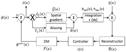
II.2 Dynamic case: closed-loop, ,
The dynamic case including loop filtering can now dealt with straightforwardly. The block diagram is depicted in Fig. 2.
Equation (1) is still valid but now is a temporally-filtered version of . Here we introduce the Laplace transform which provides a convenient treatment of the variables oppenheim97 .
We will explicitly target closed-loop systems but, as will become apparent, the formulation accommodates the open-loop as a special case.
The closed-loop transfer function between the corrective and input phase is given by madec99
| (9) |
where is the Laplace transform variable, with as the temporal frequency in , such that , i.e. each spatial mode is temporally-filtered by functions where we explicitly show the dependence on to include for instance a mode-by-mode loop gain. In Eq. (9), is the open-loop transfer function which includes pure loop time delays, WFS integration time and other filtering aspects such as the digital-to-analog conversion and the possible negative-feedback regulator for the closed-loop case. The mathematical form of these transfer functions is given in detail in Sec. II.3. At this point one can easily see that to obtain the open-loop filtering it suffices to replace by .
The transfer function of the noise relates the final phase error to the initial noise, and describes the propagation of the noise through the loop
| (10) |
where is the noise transfer function, obtained from by removing the WFS contribution (see Sec. II.3).
Therefore in closed-loop the term
| (11) |
is computed using the temporally-filtered wave-fronts
| (12) |
The spatial transfer function at every spatial frequency is evaluated from the temporal transfer function
| (13) |
where and the wind velocity vector for the layer of the atmosphere. The minus sign within the function brackets is due to the transformation from temporal to spatial variables using the frozen flow hypothesis, i.e. . Thus positive time-delay is factored in as which has a positive exponent.
For the general case with a stratified atmosphere, we now introduce the functions
| (14) |
and
| (15) |
as weighted averages over the atmospheric layers, , each with it’s own wind speed () and fractional strength (), insuring . Plugging Eq. (12) into Eq. (11) and further developing the terms yields the following relationships for the expected value of the filtered wave-fronts as
| (16) |
and
| (17) |
the cross-term between the unfiltered wave-front and its filtered version ellerbroek05 ; clare06 .
With these definitions we now have
| (18) |
The aliasing term is modified to account for the recursive filtering of the loop
| (19) |
as well as the noise propagation term:
| (20) |
where
| (21) |
is the noise transfer computed from similarly to the calculation for the wave-front; on the right-hand side of Eq. (20) is the measurement noise variance, the normalisation by comes from the 2D integration within the correctable band and is the noise propagation factor
| (22) |
which provide amore accurate numerical evaluation accounting for the loop rejection at very low temporal frequencies.
It may be convenient to include some degree of uncertainty on our knowledge of both the wind-speed and wind-direction ellerbroek05 ; clare06 taking an average over the range of possible values
| (23) |
In Eq. (23) , is the wind-speed variation during the integration and are the bounds for the wind direction and
| (24) |
to give further flexibility evaluating the final error budgets.
We further note that computing can also be achieved by computing directly the error functions . In such case the residual error is computed as the uncorrected wave-front filtered by the loop’s rejection transfer function. The closed-loop case is
| (25) |
leading as expected to a subtraction of a temporally-filtered version of the wave-front from its original value as done repeatedly throughout this presentation.
For off-axis observations, an anisoplanatic filter of the form
| (26) |
is multiplied out by Eq. (14), where is the direction vector of the off-axis star and is the altitude of the atmospheric layer.
II.3 Transfer-functions
We assume the loop transfer function can be simplified to three components, namely the WFSs, the digital-to-analog converters (DACs) and the controllers roddier99 . This by no means precludes the future inclusion of further transfer functions representative of other devices in the AO loop.
The time-delays in the loop relate to the WFS integration and to the RTC reconstruction and control (R&C) . The transfer functions for the WFS and DAC are
| (27) |
where is the integration time. If we now put together the DAC and WFS TFs, recalling the relationships and . we get
| (28) |
which effectively introduces a one-step delay. The term is customarily dropped out since at low-frequencies (compared to ) its magnitude is roughly equal to 1.
The open-loop transfer function is consequently
| (29) |
where is the controller’s transfer function for which several options are discussed further below.
A discrete-time model is conveniently expressed in the Z-domain oppenheim97
| (30) |
In a relatively standard case, the delays are taken to be equivalent to 2 frames roddier99 for which we set .
III Controller synthesis
III.1 State-space-based LQG controllers
The derivation of the Linear-Quadratic-Gaussian (LQG) controller for AO applications has been presented in detail elsewhere for both the infinitely fast DM response and otherwise correia10a . In this paper we take a shorter path and refer the reader to the bibliographic references on this particular subject for a more in-depth derivation.
The discrete-time LQG regulator minimises the cost function
| (31) |
where the weighting matrices are to be specified by developing an AO-specific Strehl-optimal quadratic criterion subject to the state-space model
| (32) |
where is the state vector that contains the wave-front coefficients (or any linearly related variables), are the noisy measurements provided by the WFS in the guide-star (GS) direction; and are spectrally white, Gaussian-distributed state excitation and measurement noise respectively. In the following we assume that , are known and that . The definition of the model parameters {} is obtained from physical modelling of the system dynamics and response functions correia10a .
We also take the case where is a delay operator that acts upon . For instance if , then with abuse of mathematical notation .
We next provide a model for a distributed Kalman-filter (DKF) that assumes a basis of complex exponential functions massioni11 ; poyneer05 , creating oscillatory modes
| (33) |
that when discretised are used to construct a mode-by-mode complex-valued state-space model as shown below. Note that this model is computed on mode-per-mode fashion, leading to many parellel calculations of small-scale, independent controllers (hence the designation distributed)
We define the state as a concatenation of complex-valued variables
| (34) |
| (35) |
with a diagonal matrix concatenating the -layers translation coefficients such that
| (36) |
where is a real-valued scalar smaller than unity that ensures overall controller stability correia10a and with the temporal frequency vector . The operation extracts and concatenates in a row-vector the diagonal coefficients of , representing the accumulation of wave-fronts at the telescope pupil-plane, i.e. .
Matrices
| (37) |
| (38) |
| (39) |
| (40) |
are chosen following the disturbance-rejection mode of the AO dynamical control problem correia10a .
The choice of model in Eqs. (39) and (40) where the Kalman filter takes into account the spatial filtering provided by gives us the possibility to chose spatial reconstructors to mitigate aliasing correia14a .
The treatment of the aliasing term provided here is formulated in its spatial dimension instead of temporal poyneer10 . The filter that is obtained is therefore more compact and lends itself more suitably to real-time implementation (in the discrete version). This choice is different from the one in Poyneer et al poyneer10 where an augmented state is suggested to accommodate the aliasing modes; this would have the downside of increasing the state dimensions considerably, by a factor of 5 if only the direct neighbours whose frequencies fold-in to the AO correctable band are considered (i.e. with , , , ) and by a factor of 9 if the cross terms where to be considered.
The implementation of the KF involves a real-time state update and prediction equations
| (41a) | ||||
| (41b) | ||||
where is the asymptotic Kalman gain computed from the solution of an estimation Riccati equation correia10a .
In order to evaluate the AO residuals with the DKF, its transfer function must be developed. This is accomplished next.
Property III.1
LQG transfer functions.
Let the general controller be a transfer function such that
| (42) |
where is the output (commands) and is the inputs (measurements).
For an LQG using the estimator version, the LQG controller transfer function is
| (43) |
where
| (44) |
Demonstration is provided in Appendix A.
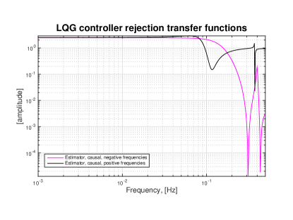
Figure 3 illustrates the rejection transfer function for a DKF controller encompassing a 3-layer atmosphere with , , , leading to 3 notches at temporal frequencies .
III.2 Integral action controllers
The commonly used integrator can be formulated from the state-space model kulcsar09 but we take a shorter path stating only the more convenient final formulation as follows
| (45) |
with the integrator gain chosen to ensure the best performance within the stability bounds.
IV Shack-Hartmann-based classical and extreme AO
A comprehensive presentation of the treatment that follows can be found in full in correia14a . Here we jump straight to the main result which is the filter formulation of the Shack-Hartmann gradients roddier99 ; rigaut98 ; hardy98 in the spatial-frequency domain.
Let the SH-WFS measurements be given by the geometrical-optics linear model
| (46) |
relating aperture-plane wave-fronts to measurements through , a phase-to-slopes linear operator over a bi-dimensional space indexed by at time ; represents white noise due to photon statistics, detector read noise and background photons. Both and are zero-mean functions of Gaussian probability distributions and known covariance matrices: and respectively. Additive, Gaussian-distributed noise is assumed both temporally and spatially uncorrelated. Variances are evaluated following formulae in thomas06 for shot photon and read noise on centre-of-gravity centroiding of SH spots
| (47) |
| (48) |
where
-
•
is the number of photons per sub-aperture and exposure
-
•
is the standard deviation of the read-out noise per pixel and per exposure
-
•
is the spot’s FWHM in number of pixels
-
•
is the sub-aperture’s FWHM in number of pixels
-
•
is the linear size of the window where the CoG is computed
The total number of photons is computed from , where is the number of photons//second emanating from the source with a zero-point of in the R band (). Furthermore we have taken .
Developing the linear operator , it can be shown that
| (49) |
where is a 2-dimensional convolution product, is a point-wise multiplication and is the unit rectangle separable function
| (50) |
is a comb function that represents the sampling process, i.e. picking sample measurements at the corners of each sub-aperture following the Fried measurement geometry.
Using common transform pairs for the individual operations (see e.g. oppenheim97 ), the Fourier representation of the measurement yields
| (51) |
where represents the continuous Fourier transform, is the frequency vector and . In Eq. (51) the gradient-taking part is
| (52) |
and the spatial averaging process is
| (53) |
The temporal integration function reads
| (54) |
on account of the frozen-flow assumption made earlier. We note that only acts as a filtering function for functions within the AO correctable band correia14a .
The Fourier-domain representation of Eq. (46) is then
| (55) |
where represents variables within a selection of frequencies , thus obtaining
| (56) |
and an aliasing term seen as the folded measurements beyond the AO cut-off frequency over spatial modes within the band
| (57) |
V Limiting post-coronagraphic contrast under predictive closed-loop control
With the previous developments, we can now investigate the impact of optimal time and spatial filtering when compared to standard least-squares, integrator-based controllers.
Using the Taylor expansion of the point-spread function (PSF) in perrin03 but including phase-only effects, for the sake of the discussion we assume that a coronagraph is capable of completely removing the two first terms (the diffraction and pinned-speckles term), leaving a halo term that is essentially the power spectrum of the wave-front aberrations macintosh05 .
Under these assumptions, the post-coronagraphic intensity relates to variance by
| (58) |
where is the variance of spatial mode indexed by frequency and is the post-coronagrahic intensity pattern (image) in the focal plane.
From Eq. (58) it can readily be seen that the post-coronagraphic image is proportional to the post-AO residual PSD. A more complete treatment can be found in herscovici17 , which provides an analytic expression for long-exposure post-coronagraphic images through turbulence but was not adopted here.
Post-coronagraphic long-exposure contrast is defined as
| (59) |
where is the AO-corrected PSF with is scaled by the long-exposure Strehl-ratio . It is computed as the ratio of the AO-corrected optical transfer function (OTF) integrated over all frequencies by the diffraction-limited OTF. PSFs are computed from the power-spectral density (PSD), using well-established relationships. First we compute covariance functions from the PSDs, using the Wiener–-Khintchine theorem. Computation of the spatial structure function ensues, from which the OTF is determined. The PSF is found from the Fourier transform of the OTF.
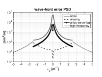
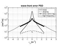
Figure 4 shows radial slabs of the residual spatial PSDs for the 4 individual error terms considered. One can see the enhanced rejection of errors close to the AO cut-off frequency for both aliasing and noise, leading to overall better performance in terms of wave-front residual and contrast across the AO-corrected field. The case considered is a 8 m telescope with 40 sub-apertures SH-WFS observing a magnitude 12 star in the R-band through a stratified atmosphere with 9 layers with and outer scale with AO cut-off .
In passing, we note that when properly scaling the residual PSDs according to (58) gives the limiting post-coronagraphic for the ideal coronagraph. We add to the work of guyon05 where the term accounts for the effect of WFS noise and time lag, the filtering of the closed-loop controller and the propagation of aliasing for the case of a stratified atmosphere.
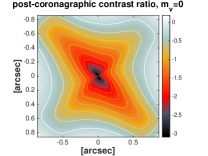
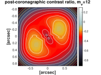
Figure 5 shows ratios of constrast obtained from Eq. (59) for the integrator controller with least-squares phase reconstruction against the DKF with minimum-variance reconstructor, i.e. . On the bright star end improvement of 2 orders of magnitude could be attained at 2-5 for existing high-contrast imagers on a 10 m-class telescope whereas one order of magnitude can still be achieved at separations closer to the AO control radius on a 12th magnitude star, on accound of better aliasing handling by the DKF.
VI Keck’s NIRC2 performance and post-coronagraphic contrast enhancement
In this section we have focused on the W. M. Keck–II NIRC2 AO system as a baseline configuration. Table 1 gathers the main parameters used to produce these results.
In Table 2 the error terms for different control systems are summarised, 3 instances of an integrator controller and a Discrete Kalman Filter (DKF).
| Telescope | |
|---|---|
| D | 11.25 m |
| throughput | 50% |
| Guide-star | |
| zenith angle | 0 deg |
| magnitude | 8 |
| Atmosphere | |
| 16 cm | |
| 75 m | |
| Fractional | [0.517, 0.119, 0.063, |
| 0.061, 0.105, 0.081, 0.054] | |
| Altitudes | [0,0.5, 1, 2, 4, 8, 16] km |
| wind speeds | [6.7, 13.9, 20.8, 29.0, |
| 29.0, 29.0, 29.0] m/s | |
| wind direction | [ |
| ] rad | |
| Wavefront Sensor | |
| Order | 2020 |
| RON | 4.5 e- |
| 12 | |
| 500 Hz | |
| 0.64 m | |
| Centroiding algorithm | thresholded CoG |
| DM | |
| Order | 2121 |
| AO loop | |
| pure delay | 4 ms |
| Imaging Wavelength | |
| (H-band) | 1.65 m |
| Error term | Int+LS | Int+MV | Int+AA | DKF+LS | DKF+Rigaut | DKF+AA |
|---|---|---|---|---|---|---|
| Aliasing | 55.4 | 55.1 | 43.7 | 56.0 | 55.7 | 44.1 |
| Aniso-servo-lag | 61.0 | 60.9 | 66.2 | 1.1 | 1.5 | 32.0 |
| WFS noise | 13.6 | 13.6 | 12.9 | 18.9 | 18.9 | 18.1 |
| Total | 83.5 | 83.3 | 80.4 | 59.1 | 58.8 | 57.4 |
| Total + Fitting | 141.2 | 141.0 | 139.4 | 128.3 | 128.2 | 127.5 |
| SR @1.65 | 77.2% | 77.2% | 77.9% | 81.1% | 81.1 % | 81.4% |
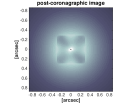
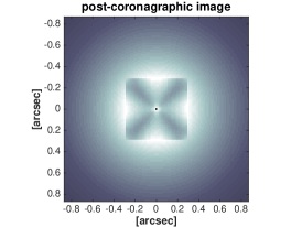
The use of the DKF results in a significant drop in the aniso-servo-lag error, as expected, becoming negligible compared to the other errors present in the system (under the assumption of perfect knowledge of wind parameters). Figure 6 shows the PSF obtained with a DKF with anti-aliasing reconstructor.
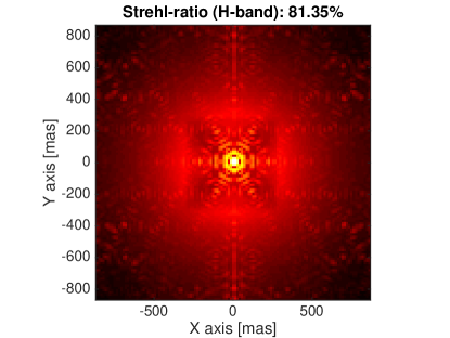
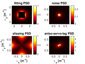
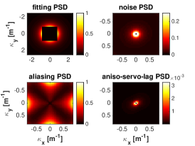
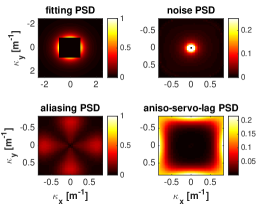
Figure 7 depicts the 2D PSDs for each error term, used here as a 1st-order approximation of an ideal post coronagraph image as per Eq. (58) for the different controllers considered sauvage16 . The fitting PSD depicts the high frequency error, or fitting error, and in all cases is zero within the correctable band and then follows the trend of the turbulent phase PSD, . All other errors affect only the correctable band () and only this region is depicted. The noise PSD follows a trend resulting from the spatial integration through .
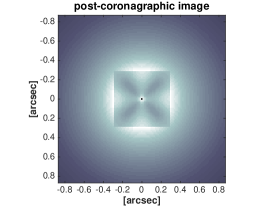
The aliasing PSD in Fig. 7 demonstrates the classic shape of an aliased post-coronagraphic image, with the largest errors towards the edges of the correctable band in a cross-like pattern. This can be somewhat mitigated by using an anti-aliasing filter (Fig. 7–right). Finally the servo-lag PSD shows two distinct lobes in the integrator case (Fig. 7-left), the direction of which is correlated with the predominant wind speed and direction weighted by the relative layer strength (typically the elongation will follow the wind at the ground), with the overall scale related to the wind speed compared with the AO system’s frame-rate. High wind-speeds or large time delays will incur larger errors here. The final images show the sum of these error as an estimation of the post-coronagraphic PSF.
Comparing the DKF to the integrator, one can readily observe the tremendous reduction in servo-lag error. With the DKF with perfect knowledge of the system and atmospheric parameters (see entry aniso-servo-lag in Table 2) it is practically reduced to null. The estimated PSF images show the AO-corrected PSF over a field 5 times larger than the AO-corrected field. For this example the strong winds at the lower layers induce a stretching of the PSF with an integrator controller (as seen in Fig. 7). The ideal case when the turbulence layer strengths, speeds and directions are known is shown as a limiting case. The image within the correction-band becomes much sharper when the DFK is utilised.
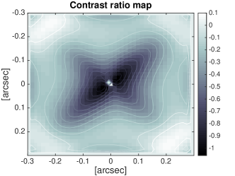
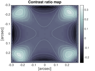
The improvement in contrast is illustrated in Fig. 8. This demonstrates the significant improvement of the DKF over an integrator controller, nearly a factor of 10 improvement in contrast close to the halo (see magnitude and noise levels on Table 2). When the DKF is coupled with the anti-aliasing reconstructor, it can still improve contrast in some areas, particularly so where aliasing is stronger at the edges of the AO control region at the expense of lower constrast in other regions.
The anti-aliasing filter used in this example does not include the effect of temporal filtering on the aliasing errors (only the open loop aliasing propagation) and hence does not improve performance over the entire correction band. Optimisation of the aliasing regularisation term would require iterative non-linear minimisation routines to chose the best term on both temporal and spatial frequencies; we leave these developments for a subsequent analysis.
 |
 |
 |
 |
 |
 |
 |
 |
VII Summary
We provide a general formulation for evaluating AO-related wave-front residuals in the spatial-frequency domain. We start by outlining how the spatio-temporal nature of the wave-front can be integrated on a controller for optimised rejection, developing power-spectral density formulae for four main error items: fitting, aliasing, noise and aniso-servo-lag. We show how any of these three errors can be rejected optimally using an anti-aliasing Wiener filter coupled to a predictive closed-loop controller. We provide a suitable formulation for the Distributed-Kalman-Filter (DKF) which is synthesised in parallel, mode-by-mode, under a flexible and convenient state-space framework for the stratified atmosphere case.
Assuming perfect knowledge of the wind at all heights, the DKF with anti-aliasing Wiener filter allows for Strehl-optimal performance, achieving the best trade-off between aliasing, noise and aniso-servo-lag errors. Post-facto aliasing rejection may be particularly useful when optical spatial filters are of little practical use and one relies therefore solely on numerical processing of signals.
We show that contrast improvements of up to three orders of magnitude can be achieved on 10 m-class telescopes with a 0-magnitude star at few separation, typically . For the Keck-II AO system, we show a wave-front error reduction of 60 nm rms leading to contrast enhancement of roughly one order of magnitude at separations , by removing the ”butterfly”-shaped servo-lag residual commonly observed in high-contrast imaging.
Finally, the developments herein can be straightforwardly used to obtaining the real-time optimal controller and the power-spectral densities used as filters when reconstructing the AO-corrected PSF from system telemetry.
VIII Software packages
All the simulations and analysis were done with the object- oriented Matlab AO simulator (OOMAO) conanr14 . The class
spatialFrequencyAdaptiveOptics implementing the analytics
developed in this paper as well as the results herein is packed with
the end-to-end library freely available from
\htmladdnormallinkhttps://github.com/cmcorreia/LAM-Publichttps://github.com/cmcorreia/LAM-Public.
Acknowledgements
The research leading to these results received the support of the A*MIDEX project (no. ANR-11-IDEX-0001- 02) funded by the ”Investissements d’Avenir” French Government program, managed by the French National Research Agency (ANR).
References
- (1) C. M. Correia and J. Teixeira, “Anti-aliasing Wiener filtering for wave-front reconstruction in the spatial-frequency domain for high-order astronomical adaptive-optics systems,” Journal of the Optical Society of America A 31, 2763 (2014).
- (2) F. J. Rigaut, J.-P. Véran, and O. Lai, “Analytical model for Shack-Hartmann-based adaptive optics systems,” in “Proc. of the SPIE,” , vol. 3353, D. Bonaccini and R. K. Tyson, eds. (SPIE, 1998), vol. 3353, pp. 1038–1048.
- (3) R. Flicker, “Analytical evaluations of closed-loop adaptive optics spatial power spectral densities,” Tech. rep., W. M. Keck Observatory (2007).
- (4) L. Jolissaint, “Synthetic modeling of astronomical closed loop adaptive optics,” Journal of the European Optical Society - Rapid publications, 5, 10055 5 (2010).
- (5) B. L. Ellerbroek, “Linear systems modeling of adaptive optics in the spatial-frequency domain,” J. Opt. Soc. Am. A 22, 310–322 (2005).
- (6) F. J. Rigaut, B. L. Ellerbroek, and R. Flicker, “Principles, limitations, and performance of multiconjugate adaptive optics,” in “Proc. of the SPIE,” , vol. 4007 (2000), vol. 4007, pp. 1022–1031.
- (7) D. T. Gavel, “Tomography for multiconjugate adaptive optics systems using laser guide stars,” in “Proc. of the SPIE,” , vol. 5490, pp. 1356–1373 (2004).
- (8) Y. H. Ono, C. M. Correia, D. R. Andersen, O. Lardière, S. Oya, M. Akiyama, K. Jackson, and C. Bradley, “Statistics of turbulence parameters at Maunakea using the multiple wavefront sensor data of RAVEN,” Monthly Notices of the Royal Astronomical Society,465, 4931–4941 (2017).
- (9) L. Poyneer, M. van Dam, and J.-P. Véran, “Experimental verification of the frozen flow atmospheric turbulence assumption with use of astronomical adaptive optics telemetry,” J. Opt. Soc. Am. A 26, 833–846 (2009).
- (10) L. A. Poyneer, B. A. Macintosh, and J.-P. Véran, “Fourier transform wavefront control with adaptive prediction of the atmosphere,” J. Opt. Soc. Am. A 24, 2645–2660 (2007).
- (11) P. Massioni, C. Kulcsár, H.-F. Raynaud, and J.-M. Conan, “Fast computation of an optimal controller for large-scale adaptive optics,” J. Opt. Soc. Am. A 28, 2298–2309 (2011).
- (12) A. V. Oppenheim and A. S. Willsky, Signals & Systems (Prentice-Hall,Inc., 1997), 2nd ed.
- (13) A. V. Oppenheim and R. W. Schafer, Discrete-time signal processing (Prentice-Hall,Inc., 1999), 2nd ed.
- (14) L. A. Poyneer and B. Macintosh, “Spatially filtered wave-front sensor for high-order adaptive optics,” J. Opt. Soc. Am. A 21, 810–819 (2004).
- (15) J.-F. Sauvage, T. Fusco, C. Petit, A. Costille, D. Mouillet, J.-L. Beuzit, K. Dohlen, M. Kasper, M. Suarez, C. Soenke, A. Baruffolo, B. Salasnich, S. Rochat, E. Fedrigo, P. Baudoz, E. Hugot, A. Sevin, D. Perret, F. Wildi, M. Downing, P. Feautrier, P. Puget, A. Vigan, J. O’Neal, J. Girard, D. Mawet, H. M. Schmid, and R. Roelfsema, “SAXO: the extreme adaptive optics system of SPHERE (I) system overview and global laboratory performance,” Journal of Astronomical Telescopes, Instruments, and Systems 2, 025003 (2016).
- (16) O. Guyon, “Limits of adaptive optics for high-contrast imaging,” The Astrophysical Journal 629, 592 (2005).
- (17) L. A. Poyneer and J.-P. Véran, “Toward feasible and effective predictive wavefront control for adaptive optics,” in “Proc. of the SPIE - Adaptive Optical Systems,” , vol. 7015, N. Hubin, C. E. Max, and P. L. Wizinowich, eds. (SPIE, 2008), vol. 7015, p. 70151E.
- (18) P.-Y. Madec, Adaptive Optics for Astronomy (Cambridge University Press, New York, 1999), chap. Control Techniques.
- (19) R. M. Clare, B. L. Ellerbroek, G. Herriot, and J.-P. Véran, “Adaptive optics sky coverage modeling for extremely large telescopes,” Appl. Opt. 45, 8964–8978 (2006).
- (20) F. Roddier, Adaptive Optics in Astronomy (Cambridge University Press, New York, 1999).
- (21) C. Correia, H.-F. Raynaud, C. Kulcsár, and J.-M. Conan, “On the optimal reconstruction and control of adaptive optical systems with mirroir dynamics,” J. Opt. Soc. Am. A 27, 333–349 (2010).
- (22) L. A. Poyneer and J.-P. Véran, “Optimal modal Fourier-transform wavefront control,” J. Opt. Soc. Am. A 22, 1515–1526 (2005).
- (23) L. A. Poyneer and J.-P. Véran, “Kalman filtering to suppress spurious signals in adaptive optics control,” J. Opt. Soc. Am. A 27, A223–A234 (2010).
- (24) C. Kulcsár, H.-F. Raynaud, J.-M. Conan, C. Correia, and C. Petit, “Control design and turbulent phase models in adaptive optics: A state-space interpretation,” in “Adaptive Optics: Methods, Analysis and Applications,” (Optical Society of America, 2009), p. AOWB1.
- (25) J.W.Hardy, Adaptive Optics for Astronomical Telescopes (Oxford, New York, 1998).
- (26) S. Thomas, T. Fusco, A. Tokovinin, M. Nicolle, V. Michau, and G. Rousset, “Comparison of centroid computation algorithms in a Shack-Hartmann sensor,” Monthly Notices of the Royal Astronomical Society, 371, 323–336 (2006).
- (27) M. D. Perrin, A. Sivaramakrishnan, R. B. Makidon, B. R. Oppenheimer, and J. R. Graham, “The structure of high strehl ratio point-spread functions,” The Astrophysical Journal 596, 702 (2003).
- (28) B. Macintosh, L. Poyneer, A. Sivaramakrishnan, and C. Marois, “Speckle lifetimes in high-contrast adaptive optics,” (2005).
- (29) O. Herscovici-Schiller, L. M. Mugnier, and J.-F. Sauvage, “An analytic expression for coronagraphic imaging through turbulence. Application to on-sky coronagraphic phase diversity,” Monthly Notices of the Royal Astronomical Society, 467, L105–L109 (2017).
- (30) R. Conan and C. Correia, “Object-oriented Matlab adaptive optics toolbox,” in “Society of Photo-Optical Instrumentation Engineers (SPIE) Conference Series,” , vol. 9148, p. 6 (2014).
Appendix A LQG transfer functions
-
Example
LQG transfer functions.
The state-update and state-estimate equations of the LQG are
(62) The second line of Eq. (62) can be likewise written, using and the -transforms of and respectively.
(63) Let’s start by assuming that the state cannot be attained by the controls, i.e. . It is generalized afterwards.
Multiplying out by on both sides, one gets
(64) With this result and the second line in Eq. (62)
(65) Using a command vector , i.e. a causal form for the controls, one gets
(66) where
(67) from which the controller transfer function writes
(68) If instead we were to compute then
(69) Grouping terms, one gets
(70) The controller transfer function is finally written as
(71) The general case in predictor form with an arbitrary delay and one gets
(72) For a command vector in estimator form , following an analogous reasoning
(73) yielding
(74) Grouping terms
(75) with
(76) The general case when and arbitrary delay equates to
(77)