$J/{\psi}$ ${\to}$ $D_{s,d}{\pi}$, $D_{s,d}K$ decays with perturbative QCD approach

Abstract

Besides the conventional strong and electromagnetic decay modes, the $J/{\psi}$ particle can also decay via the weak interaction in the standard model. In this paper, nonleptonic $J/{\psi}$ ${\to}$ $D_{s,d}{\pi}$, $D_{s,d}K$ weak decays, corresponding to the externally emitted virtual $W$ boson process, are investigated with the perturbative QCD approach. It is found that branching ratio for the Cabibbo-favored $J/{\psi}$ ${\to}$ $D_{s}{\pi}$ decay can reach up to ${\cal O}(10^{-10})$, which might be potentially measurable at the future high-luminosity experiments.

I Introduction

The discovery of the $J/{\psi}$ particle in 1974 at BNL in $p$-Be collisions bnl and at SLAC in $e^{+}e^{-}$ collisions slac provides evidence of the existence of the charm quark, and verifies that the quarks are physical elementary particles rather than purely mathematical entities gell . The $J/{\psi}$ meson consists of the charm quark and antiquark pair $c\bar{c}$, so it carries some given quantum numbers, such as spin, isospin, parity, and charge conjugation, i.e., $I^{G}J^{PC}$ $=$ $0^{-}1^{--}$ pdg . The mass of $J/{\psi}$ meson is about three times the proton mass, but the width of $J/{\psi}$ meson is extremely narrow, only about 30 ppm of its mass. One of the major reasons for the characteristic width is that $J/{\psi}$ ${\to}$ $D\overline{D}$ is forbidden inasmuch as the $J/{\psi}$ meson lies below the kinematic $D\bar{D}$ threshold, and it is required by the $C$-parity conservation and the sacrosanct spin-statistics theorem that the $J/{\psi}$ meson must strongly decay into light hadrons via the $c\bar{c}$ annihilation into three gluons, which is of higher order in the quark-gluon coupling ${\alpha}_{s}$ and is therefore suppressed by the phenomenological Okubo-Zweig-Iizuka (OZI) rules o ; z ; i .

The $J/{\psi}$ decay modes are usually partitioned into four categories: hadronic decay $J/{\psi}$ ${\to}$ $ggg$ with branching ratio ${\sim}$ $(64.1{\pm}1.0)\%$ pdg , electromagnetic decay $J/{\psi}$ ${\to}$ ${\gamma}^{\ast}$ with branching ratio ${\sim}$ $(2+R){\cal B}r_{ee}$, radiative decay $J/{\psi}$ ${\to}$ ${\gamma}gg$ with branching ratio ${\sim}$ $(8.8{\pm}1.1)\%$ pdg , and magnetic dipole transition decay $J/{\psi}$ ${\to}$ ${\gamma}{\eta}_{c}$ with branching ratio ${\sim}$ $(1.7{\pm}0.4)\%$ pdg , where the ratio of the production cross section $R$ $=$ ${\sigma}(e^{+}e^{-}{\to}X)/{\sigma}(e^{+}e^{-}{\to}{\mu}^{+}{\mu})$ and ${\cal B}r_{ee}$ is the branching ratio for the pure leptonic $J/{\psi}$ ${\to}$ $e^{+}e^{-}$ decay. Because of OZI rule violation, the electromagnetic $J/{\psi}$ decay can compete favorably with hadronic $J/{\psi}$ decay. The properties of gluons and the quark-gluon coupling can be collected in hadronic and radiative $J/{\psi}$ decay. In addition, the radiative $J/{\psi}$ decay offers an ideal plaza to search for possible glueballs. Besides, the $J/{\psi}$ decay via the weak interaction is permissible within the standard model. In this paper, we will investigate the charm-changing nonleptonic $J/{\psi}$ ${\to}$ $D_{s,d}{\pi}$, $D_{s,d}K$ weak decays with the perturbative QCD (pQCD) approach pqcd1 ; pqcd2 ; pqcd3 . Our motivation is listed as follows.

Experimentally, (1) thanks to the tremendous impetus from BES, CLEO-c, B-factories, LHCb, and so on, the $J/{\psi}$ particle attracts much persistent attention of experimentalists and theorists. A large amount of $J/{\psi}$ data samples have been accumulated. It is promisingly expected to produce about $10^{10}$ $J/{\psi}$ samples at BESIII per year with the designed luminosity cpc36 , and over $10^{10}$ prompt $J/{\psi}$ samples at LHCb per $fb^{-1}$ data epjc71 . It is not utopian to carefully scrutinize the $J/{\psi}$ weak decays at the high-luminosity dedicated experiments in the future. (2) The production and “flavor tag” of single charged $D$ meson from $J/{\psi}$ decay will single the potential signal out from massive and intricate background. Recently, the $J/{\psi}$ ${\to}$ $D_{s}{\rho}$, $D_{u}K^{\ast}$ decays have been investigated at BESIII using $2.25{\times}10^{8}$ $J/{\psi}$ data samples prd89.071101 , although no evidence is found due to tiny accident probabilities and insufficient available data samples. It is hard but interesting to hunt for $J/{\psi}$ weak decay experimentally. A deviant production rate of single $D$ meson from $J/{\psi}$ decay would be a hint of new physics.

Theoretically, the $J/{\psi}$ ${\to}$ $D_{q}P$ decay is induced by $c$ ${\to}$ $q$ $+$ $W^{+}$ transition, where $q$ $=$ $s$ and $d$, and the virtual $W^{+}$ boson materializes into a pair of quarks which then grows into a pseudoscalar meson $P$ $=$ ${\pi}$ and $K$. As it is well known, nonleptonic $J/{\psi}$ weak decay must be with the participation of the strong interaction, and the $c$ quark mass is between nonperturbative and perturbative domain. Recently, many QCD-inspired methods have been developed, such as the pQCD approach pqcd1 ; pqcd2 ; pqcd3 , the QCD factorization (QCDF) approach qcdf1 ; qcdf2 ; qcdf3 , the soft and collinear effective theory scet1 ; scet2 ; scet3 ; scet4 , and have been applied preferably to accommodate measurements on nonleptonic $B$ decays. Based on collinear approximation, the $J/{\psi}$ ${\to}$ $DP$ decays have been studied with naive factorization plb252 ; ijmpa14 ; ahep2013 and the QCDF approach ijmpa30 , where theoretical results differ mainly from hadronic input parameters. In this paper, the $J/{\psi}$ ${\to}$ $D_{s,d}P$ decays will be studied with the pQCD approach based on $k_{T}$ factorization. It is expected that with nonleptonic $J/{\psi}$ weak decay, one can glean new insights into the factorization mechanism, nonfactorizable contributions, nonperturbative dynamics, final state interactions, and so on.

This paper is organized as follows. In section II, we present the theoretical framework and the amplitudes for the $J/{\psi}$ ${\to}$ $D_{s,d}P$ decay with the pQCD approach. Section III is devoted to numerical results and discussion. The last section is our summary.

II theoretical framework

II.1 The effective Hamiltonian

Constructed by means of the operator product expansion and the renormalization group (RG) method, the effective Hamiltonian describing the $J/{\psi}$ ${\to}$ $D_{s,d}P$ weak decay could be written as a series of effective local operators $Q_{i}$ multiplied by effective Wilson coefficients $C_{i}$ and have the following structure 9512380 :

$${\cal H}_{\rm eff}\ =\ \frac{G_{F}}{\sqrt{2}}\,\sum\limits_{q_{1},q_{2}}V_{cq_{1}}V_{uq_{2}}^{\ast}\,\Big{\{}C_{1}({\mu})\,Q_{1}({\mu})+C_{2}({\mu})\,Q_{2}({\mu})\Big{\}}+{\rm h.c.},$$ (1)

where $G_{F}$ is the Fermi coupling constant and $q_{1,2}$ $=$ $d$, $s$.

Using the Wolfenstein parameterization prl51 , there are some hierarchy relations among the Cabibbo-Kobayashi-Maskawa prl10 ; ptp49 (CKM) factors, i.e.,

$$V_{cs}V_{ud}^{\ast} = 1-{\lambda}^{2}-\frac{1}{2}A^{2}{\lambda}^{4}+{\cal O}({\lambda}^{6}),$$ (2)

$$V_{cs}V_{us}^{\ast} = {\lambda}-\frac{1}{2}{\lambda}^{3}-\frac{1}{8}{\lambda}^{5}(1+4A^{2})+{\cal O}({\lambda}^{6}),$$ (3)

$$V_{cd}V_{ud}^{\ast} = -V_{cs}V_{us}^{\ast}-A^{2}{\lambda}^{5}({\rho}+i{\eta})+{\cal O}({\lambda}^{6}),$$ (4)

$$V_{cd}V_{us}^{\ast} = -{\lambda}^{2}+{\cal O}({\lambda}^{6}),$$ (5)

for $J/{\psi}$ ${\to}$ $D_{s}{\pi}$, $D_{s}K$, $D_{d}{\pi}$, $D_{d}K$ decays, respectively, where the Wolfenstein parameter ${\lambda}$ $=$ ${\sin}{\theta}_{c}$ ${\simeq}$ $0.2$ pdg and ${\theta}_{c}$ is the Cabibbo angle.

The auxiliary scale ${\mu}$ in Eq.(1) factorizes contributions into long- and short-distance dynamics. The Wilson coefficients $C_{1,2}(\mu)$ summarize the short-distance physical contributions above the scales of ${\mu}$. They are computable at the scale of the $W$ boson mass ${\mu}$ $=$ ${\cal O}(m_{W})$ with perturbation theory, and then evolved down to a characteristic scale for $c$ quark decay.

$$\vec{C}({\mu})=U_{4}({\mu},m_{b})U_{5}(m_{b},m_{W})\vec{C}(m_{W}),$$ (6)

where $U_{f}({\mu}_{f},{\mu}_{i})$ is the RG evolution matrix transforming the Wilson coefficients from scale ${\mu}_{i}$ to ${\mu}_{f}$. The explicit expression of $U_{f}({\mu}_{f},{\mu}_{i})$ can be found in Ref.9512380 . The Wilson coefficients have properly been evaluated to the next-to-leading order.

The penguin contributions are severely suppressed by the CKM factors $V_{cd}V_{ud}^{\ast}$ $+$ $V_{cs}V_{us}^{\ast}$ $=$ $-V_{cb}V_{ub}^{\ast}$ ${\sim}$ ${\cal O}({\lambda}^{5})$, which are negligible in our calculation. Only the tree operators related to $W$ emission contributions are considered. The expressions of tree operators are

$$Q_{1} = [\bar{q}_{1,{\alpha}}{\gamma}_{\mu}(1-{\gamma}_{5})c_{\alpha}][\bar{u}_{\beta}{\gamma}^{\mu}(1-{\gamma}_{5})q_{2,{\beta}}],$$ (7)

$$Q_{2} = [\bar{q}_{1,{\alpha}}{\gamma}_{\mu}(1-{\gamma}_{5})c_{\beta}][\bar{u}_{\beta}{\gamma}^{\mu}(1-{\gamma}_{5})q_{2,{\alpha}}],$$ (8)

where ${\alpha}$ and ${\beta}$ are color indices and the sum over repeated indices is understood. The physical contributions below scales of ${\mu}$ are included in hadronic matrix elements (HME), where the local operators are sandwiched between initial and final hadron states. Generally, HME is the most complicated and intractable part, where the perturbative and nonperturbative effects entangle with each other. In addition, nonfactorizable corrections to HME should be taken into account decently so that the ${\mu}$ dependences of HME could cancel and/or milden those of Wilson coefficients.

II.2 Hadronic matrix elements

With the Lepage-Brodsky approach for exclusive processes prd22 , HME could be expressed as the convolution of a hard scattering kernel with distribution amplitudes (DA) in parton momentum fractions, where DA reflecting the nonperturbative contributions is commonly assumed to be universal, which makes the structure simple. The hard part could be perturbatively computed in an expansion of strong coupling ${\alpha}_{s}$. Unfortunately, soft endpoint contributions do not admit self-consistent treatment with collinear factorization approximation qcdf1 ; qcdf2 ; qcdf3 . To settle the issue, in evaluation of potentially infrared contributions with the pQCD approach, the transverse momentum of quarks are kept explicitly and the Sudakov factors are introduced for each of mesonic DA pqcd1 ; pqcd2 ; pqcd3 . Finally, the decay amplitudes could be factorized into three parts pqcd2 ; pqcd3 : the hard effects enclosed by Wilson coefficients $C_{i}$, the heavy quark decay amplitudes ${\cal H}$, and process-independent wave functions ${\Phi}$,

$${\int}dk\,C_{i}(t)\,{\cal H}(t,k)\,{\Phi}(k)\,e^{-S},$$ (9)

where $t$ is a typical scale, $k$ is the momentum of valence quarks, and the Sudakov factor $e^{-S}$ is used to suppress the long-distance contributions and makes the hard scattering subprocess more perturbative.

II.3 Kinematic variables

In the rest frame of the $J/{\psi}$ meson, kinematic variables are defined as below:

$$p_{J/{\psi}}\,=\,p_{1}\,=\,\frac{m_{1}}{\sqrt{2}}(1,1,0),$$ (10)

$$p_{D}\,=\,p_{2}\,=\,(p_{2}^{+},p_{2}^{-},0),$$ (11)

$$p_{P}\,=\,p_{3}\,=\,(p_{3}^{-},p_{3}^{+},0),$$ (12)

$$k_{i}\,=\,x_{i}\,p_{i}+(0,0,\vec{k}_{iT}),$$ (13)

$${\epsilon}_{\psi}^{\parallel}\,=\,{\epsilon}_{1}^{\parallel}\,=\,\frac{1}{\sqrt{2}}(-1,1,0),$$ (14)

$$n_{+}=(1,0,0),$$ (15)

$$n_{-}=(0,1,0),$$ (16)

$$p_{i}^{\pm}\,=\,(E_{i}\,{\pm}\,p)/\sqrt{2},$$ (17)

$$t\,=\,2\,p_{1}{\cdot}p_{2}\,=\ 2\,m_{1}\,E_{2},$$ (18)

$$u\,=\,2\,p_{1}{\cdot}p_{3}\,=\ 2\,m_{1}\,E_{3},$$ (19)

$$s\,=\,2\,p_{2}{\cdot}p_{3},$$ (20)

$$p=\frac{\sqrt{[m_{1}^{2}-(m_{2}+m_{3})^{2}]\,[m_{1}^{2}-(m_{2}-m_{3})^{2}]}}{2\,m_{1}},$$ (21)

where the subscripts $i$ $=$ $1$, $2$, $3$ on variables $p_{i}$, $E_{i}$ and $m_{i}$ correspond to $J/{\psi}$, $D$, $P$ mesons, respectively; $p_{i}$ is a four-dimensional momentum abiding by the on-shell condition $p_{i}^{2}$ $=$ $m_{i}^{2}$; $x_{i}$ and $k_{i}$ ($\vec{k}_{iT}$) denote the longitudinal momentum fraction and (transverse) momentum of a relatively light valence quark in mesons, respectively; ${\epsilon}_{1}^{\parallel}$ denotes the longitudinal polarization vector satisfying with the relations ${\epsilon}_{1}^{\parallel}{\cdot}{\epsilon}_{1}^{\parallel}$ $=$ $-1$ and ${\epsilon}_{1}^{\parallel}{\cdot}p_{1}$ $=$ $0$; $n_{+}$ and $n_{-}$ are the plus and minus null vectors, respectively, complying with $n_{\pm}^{2}$ $=$ $0$ and $n_{+}{\cdot}n_{-}$ $=$ $1$; $t$, $u$, and $s$ are the Lorentz-invariant variables; and $p$ is the common momentum of the final states. The notation of momentum is displayed in Fig.2(a).

II.4 Wave functions

Taking the convention of Refs. prd65 ; npb529 , the HME of the diquark operators squeezed between the vacuum and meson state is defined as below:

$${\langle}0{|}c_{i}(z)\bar{c}_{j}(0){|}{\psi}(p_{1},{\epsilon}_{1}^{\parallel}){\rangle}=\frac{f_{\psi}}{4}{\int}d^{4}k_{1}\,e^{-ik_{1}{\cdot}z}\Big{\{}\!\!\not{\epsilon}_{1}^{\parallel}\Big{[}m_{1}\,{\Phi}_{\psi}^{v}(k_{1})-\!\!\not{p}_{1}\,{\Phi}_{\psi}^{t}(k_{1})\Big{]}\Big{\}}_{ji},$$ (22)

$${\langle}D_{q}(p_{2}){|}\bar{q}_{i}(z)c_{j}(0){|}0{\rangle}=\frac{if_{D_{q}}}{4}{\int}d^{4}k_{2}\,e^{ik_{2}{\cdot}z}\,\Big{\{}{\gamma}_{5}\Big{[}\!\!\not{p}_{2}\,{\Phi}_{D}^{a}(k_{2})+m_{2}\,{\Phi}_{D}^{p}(k_{2})\Big{]}\Big{\}}_{ji},$$ (23)

$${\langle}P(p_{3}){|}q_{i}(0)\bar{q}^{\prime}_{j}(z){|}0{\rangle}=\frac{if_{P}}{4}{\int}_{0}^{1}dk_{3}\,e^{ik_{3}{\cdot}z}\Big{\{}{\gamma}_{5}\Big{[}\!\!\not{p}_{3}\,{\Phi}_{P}^{a}(k_{3})+{\mu}_{P}\,{\Phi}_{P}^{p}(k_{3})+{\mu}_{P}\,(\!\not{n}_{-}\!\!\not{n}_{+}-1)\,{\Phi}_{P}^{t}(k_{3})\Big{]}\Big{\}}_{ji},$$ (24)

where $f_{\psi}$, $f_{D_{q}}$, and $f_{P}$ are decay constants; wave functions ${\Phi}_{\psi}^{v}$ and ${\Phi}_{D,P}^{a}$ are twist-2; wave functions ${\Phi}_{\psi}^{t}$ and ${\Phi}_{D,P}^{p,t}$ are twist-3. For the $J/{\psi}$ meson, the transverse polarization components contribute nothing to decay amplitudes in question.

The decay constant $f_{\psi}$ can be obtained from the experimental branching ratios of the electromagnetic $J/{\psi}$ decay into charged lepton pairs through the formula

$${\cal B}r(J/{\psi}{\to}{\ell}^{+}{\ell}^{-})=\frac{16{\pi}}{27}f_{\psi}^{2}\frac{{\alpha}_{\rm QED}^{2}}{m_{\psi}\,{\Gamma}_{\psi}}\sqrt{1-2\frac{m_{\ell}^{2}}{m_{\psi}^{2}}}\Big{\{}1+2\frac{m_{\ell}^{2}}{m_{\psi}^{2}}\Big{\}},$$ (25)

where ${\alpha}_{\rm QED}$ is the fine-structure constant, $m_{\ell}$ is the lepton mass and ${\ell}$ $=$ $e$, ${\mu}$. Here, we will use the weighted average decay constant $f_{\psi}$ $=$ $395.1{\pm}5.0$ MeV (see Table 1).

Table 1: Experimental branching ratios for leptonic $J/{\psi}$ decay and decay constant $f_{\psi}$, where ${\langle}f_{\psi}{\rangle}$ denotes the weighted average, and errors of decay constant arise from mass $m_{\psi}$, decay width ${\Gamma}_{\psi}$ and branching ratios.

decay mode	branching ratio	$f_{\psi}$	${\langle}f_{\psi}{\rangle}$
$J/{\psi}$ ${\to}$ $e^{+}e^{-}$	$(5.971{\pm}0.032)\%$	$395.4{\pm}7.0$ MeV	$395.1{\pm}5.0$ MeV
$J/{\psi}$ ${\to}$ ${\mu}^{+}{\mu}^{-}$	$(5.961{\pm}0.033)\%$	$394.8{\pm}7.1$ MeV

For the emitted pseudoscalar $P$ meson, only the twist-2 wave functions are involved in the actual calculation (see Appendix A). The twist-2 DA has the expansion npb529 :

$${\phi}_{P}^{a}(x)=6\,x\,\bar{x}\,\Big{\{}1+\sum\limits_{i=1}a_{i}^{P}\,C_{i}^{3/2}(t)\Big{\}},$$ (26)

where $\bar{x}$ $=$ $1$ $-$ $x$ and $t$ $=$ $1$ $-$ $2x$; Gegenbauer moments $a_{i}^{P}$ corresponding to Gegenbauer polynomials $C_{i}^{3/2}(t)$ could be determined experimentally or with nonperturbative methods (such as QCD sum rules). It follows that $a_{i}^{P}$ $=$ $0$ for odd $i$ due to the $G$-parity invariance of DA for ${\pi}$ and ${\eta}^{(\prime)}$ mesons. Gegenbauer polynomials $C_{i}^{3/2}(t)$ have the expression

$$C_{1}^{3/2}(t)=3\,t,\quad C_{2}^{3/2}(t)=\frac{3}{2}\,(5\,t^{2}-1),\quad{\cdots}$$ (27)

Because of $m_{J/{\psi}}$ ${\simeq}$ $2m_{c}$ and $m_{D_{q}}$ ${\simeq}$ $m_{c}$ $+$ $m_{q}$, it is commonly assumed that valence quarks in the charmonium $J/{\psi}$ and charmed mesons might be nearly nonrelativistic. Nonrelativistic quantum chromodynamics (NRQCD) prd46 ; prd51 ; rmp77 and the Schrödinger equation can be used to describe their spectrum. The ground state eigenfunction of the time-independent Schrödinger equation with an isotropic harmonic oscillator potential, corresponding to the quantum numbers $nL$ $=$ $1S$, has the form shown below in the momentum space,

$${\phi}_{1S}(\vec{k})\ {\sim}\ e^{-\vec{k}^{2}/2{\omega}^{2}},$$ (28)

where parameter ${\omega}$ determines the average transverse momentum, ${\langle}1S{|}k^{2}_{T}{|}1S{\rangle}$ $=$ ${\omega}^{2}$. According to the NRQCD power counting rules prd46 , the typical momentum is $k$ ${\sim}$ ${\omega}$ ${\sim}$ $mv$ ${\sim}$ $m{\alpha}_{s}$, and the quark velocity $v$ is approximately equal to the effective QCD coupling strength ${\alpha}_{s}$. Employing the substitution transformation xiao ,

$$\vec{k}^{2}\ {\to}\ \frac{1}{4}\Big{(}\frac{\vec{k}_{T}^{2}+m_{q_{1}}^{2}}{x_{1}}+\frac{\vec{k}_{T}^{2}+m_{q_{2}}^{2}}{x_{2}}\Big{)},$$ (29)

where $x_{i}$ fitting with $x_{1}$ $+$ $x_{2}$ $=$ $1$ is the longitudinal momentum fraction of valence quark with mass $m_{q_{i}}$, and then integrating out transverse momentum $k_{T}$ and combining with their asymptotic forms, one can obtain DA for $J/{\psi}$ and $D$ mesons,

$${\phi}_{\psi}^{v}(x)=A\,x\,\bar{x}\,{\exp}\Big{\{}-\frac{m_{c}^{2}}{8\,{\omega}_{1}^{2}\,x\,\bar{x}}\Big{\}},$$ (30)

$${\phi}_{\psi}^{t}(x)=B\,t^{2}\,{\exp}\Big{\{}-\frac{m_{c}^{2}}{8\,{\omega}_{1}^{2}\,x\,\bar{x}}\Big{\}},$$ (31)

$${\phi}_{D}^{a}(x)=C\,x\,\bar{x}\,{\exp}\Big{\{}-\frac{\bar{x}\,m_{q}^{2}+x\,m_{c}^{2}}{8\,{\omega}_{2}^{2}\,x\,\bar{x}}\Big{\}},$$ (32)

$${\phi}_{D}^{p}(x)=D\,{\exp}\Big{\{}-\frac{\bar{x}\,m_{q}^{2}+x\,m_{c}^{2}}{8\,{\omega}_{2}^{2}\,x\,\bar{x}}\Big{\}},$$ (33)

where parameter ${\omega}_{i}$ $=$ $m_{i}{\alpha}_{s}(m_{i})$, and coefficients of $A$, $B$, $C$, $D$ could be determined by the normalization conditions,

$${\int}_{0}^{1}dx\,{\phi}_{\psi}^{v,t}(x)=1,\quad{\int}_{0}^{1}dx\,{\phi}_{D}^{a,p}(x)=1.$$ (34)

Here, one may question the validity of the nonrelativistic treatment on wave functions of the $D$ mesons, because the motion of the light valence quark in the $D$ meson is generally assumed to be relativistic. In fact, there are several phenomenological models for $D$ meson wave functions, for example, Eq.(30) in Ref. prd78lv . The $D$ wave function, which is favored by Ref. prd78lv via fitting with measurements on the $B$ ${\to}$ $DP$ decays and often used within the pQCD framework, has the form

$${\phi}_{D}(x,b)=6\,x\bar{x}\,\Big{\{}1+C_{D}(1-2x)\Big{\}}{\exp}\Big{\{}-\frac{1}{2}w^{2}b^{2}\Big{\}},$$ (35)

where $C_{D}$ $=$ $0.4$ and $w$ $=$ $0.2$ GeV for the $D_{s}$ meson; $C_{D}$ $=$ $0.5$ and $w$ $=$ $0.1$ GeV for the $D_{d}$ meson. In addition, the same form of Eq.(35) is widely used in many practical calculation without a distinction between twist-2 and twist-3 DAs.

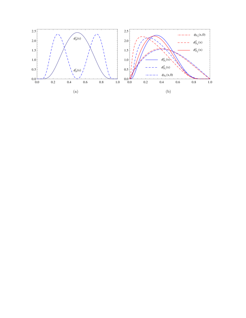
Figure 1: The shape lines of wave functions for the $J/{\psi}$ meson in (a) and the $D_{d,s}$ mesons in (b), where the expressions of ${\phi}_{\psi}^{v,t}(x)$, ${\phi}_{D}^{a,p}(x)$, and ${\phi}_{D}(x,b)$ are given in Eqs.(30—33) and Eq.(35).

The shape lines of DAs for $J/{\psi}$ and $D_{s,d}$ mesons are displayed in Fig. 1. It is clearly seen that (1) ${\phi}_{\psi}^{v,t}(x)$ for the $J/{\psi}$ meson is symmetric under the interchange of momentum fractions $x$ ${\leftrightarrow}$ $\bar{x}$, and a broad peak of ${\phi}_{D}^{a,p}(x)$ for $D$ mesons appears at the $x$ $<$ $0.5$ regions, which is basically consistent with the scenario that valence quarks in mesons might share longitudinal momentum fractions according to their masses. (2) Because of the suppression from exponential functions, DAs of Eqs.(30—33) fall quickly down to zero at endpoint $x$, $\bar{x}$ ${\to}$ $0$, which provides another effective cutoff for soft contributions. (3) The flavor symmetry breaking effects between $D_{d}$ and $D_{s}$ mesons, and the distinction between twist-2 and twist-3 DAs are apparent in Eqs.(32) and (33) rather than Eq.(35). Hence, in subsequent calculation, we will take Eqs.(32) and (33) as the twist-2 and twist-3 DA for the $D$ meson, respectively.

II.5 Decay amplitudes

The Feynman diagrams for the $J/{\psi}$ ${\to}$ $D_{s}{\pi}$ decay within the pQCD framework are shown in Fig.2, including factorizable emission topologies (a) and (b) where gluon connects $J/{\psi}$ with the $D_{s}$ meson, and nonfactorizable emission topologies (c) and (d) where gluon couples the spectator quark with the emitted pion.

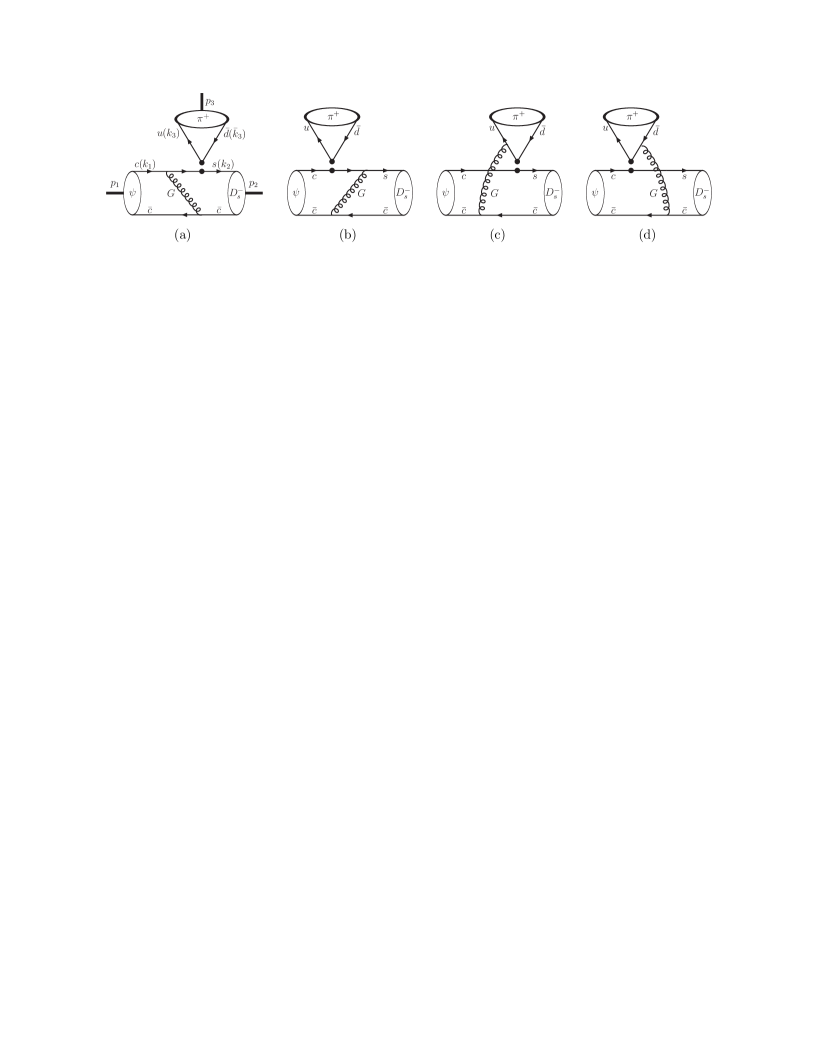
Figure 2: Feynman diagrams for the $J/{\psi}$ ${\to}$ $D_{s}{\pi}$ decay, where (a) and (b) are factorizable emission diagrams, (c) and (d) are nonfactorizable emission diagrams.

After calculation with the master pQCD formula, amplitude for $J/{\psi}$ ${\to}$ $D_{q}P$ decay is written as

$${\cal A}(J/{\psi}{\to}D_{q}P)=\frac{G_{F}}{\sqrt{2}}\,V_{cq_{1}}V_{uq_{2}}^{\ast}\,C_{{\cal A}}\sum\limits_{i}{\cal A}_{i},$$ (36)

$$C_{{\cal A}}=m_{\psi}\,({\epsilon}_{\psi}{\cdot}p_{D})\,f_{\psi}\,f_{D_{q}}\,f_{P}\,{\pi}\,C_{F}/{N_{c}},$$ (37)

where the color number $N_{c}$ $=$ $3$ and color factor $C_{F}$ $=$ $4/3$; the subscript $i$ on ${\cal A}_{i}$ corresponds to indices of Fig.2. The expressions of building blocks ${\cal A}_{i}$ can be found in Appendix A.

According to the modeling notation of Ref. zpc29 , the longitudinal axial-vector form factor $A_{0}$ for $J/{\psi}$ ${\to}$ $D_{q}$ transition is defined as

$${\langle}D(p_{2}){|}\,\bar{q}\,{\gamma}_{\mu}{\gamma}_{5}\,c\,{|}J/{\psi}(p_{1},{\epsilon}_{1}^{\parallel}){\rangle}=i\,2\,m_{\psi}\,\frac{{\epsilon}_{1}^{\parallel}{\cdot}q}{q^{2}}\,q_{\mu}\,A_{0}(q^{2}),$$ (38)

where the momentum transfer $q$ $=$ $p_{1}$ $-$ $p_{2}$. Form factor $A_{0}$ with the pQCD approach can be expressed as

$$A_{0}(q^{2})\,=\,-\frac{{\pi}\,C_{F}}{2\,N_{c}}f_{\psi}\,f_{D_{q}}\left.\Big{\{}{\cal A}_{a}+{\cal A}_{b}\Big{\}}\right|_{a_{1}=1}^{m_{3}^{2}=q^{2}}.$$ (39)

III Numerical results and discussion

In the rest frame of the $J/{\psi}$ meson, the branching ratio is defined as

$${\cal B}r(J/{\psi}{\to}DP)=\frac{1}{12{\pi}}\,\frac{p}{m_{\psi}^{2}{\Gamma}_{\psi}}\,{|}{\cal A}(J/{\psi}{\to}DP){|}^{2}.$$ (40)

Table 2: The numerical values of input parameters.

CKM parameters pdg	$A$ $=$ $0.814^{+0.023}_{-0.024}$,	${\lambda}$ $=$ $0.22537{\pm}0.00061$,
	$\bar{\rho}$ $=$ $0.117{\pm}0.021$,	$\bar{\eta}$ $=$ $0.353{\pm}0.013$,
mass and decay constants	$m_{\psi}$ $=$ $3096.916{\pm}0.011$ MeV pdg ,	$f_{\psi}$ $=$ $395.1{\pm}5.0$ MeV,
	$m_{D_{s}}$ $=$ $1968.30{\pm}0.11$ MeV pdg ,	$f_{D_{s}}$ $=$ $257.5{\pm}4.6$ MeV pdg ,
	$m_{D_{d}}$ $=$ $1869.61{\pm}0.10$ MeV pdg ,	$f_{D_{d}}$ $=$ $204.6{\pm}5.0$ MeV pdg ,
	$m_{c}$ $=$ $1.67{\pm}0.07$ GeV pdg ,	$f_{K}$ $=$ $156.2{\pm}0.7$ MeV pdg ,
	$m_{s}$ ${\approx}$ $510$ MeV uds ,	$f_{\pi}$ $=$ $130.41{\pm}0.20$ MeV pdg ,
	$m_{d}$ ${\approx}$ $310$ MeV uds ,	${\Gamma}_{\psi}$ $=$ $92.9{\pm}2.8$ keV pdg ,
Gegenbauer moments npb529	$a_{1}^{K}$ $=$ $-0.06{\pm}0.03$,	$a_{2}^{{\pi},K}$ $=$ $0.25{\pm}0.15$.

Table 3: Form factor $A_{0}^{J/{\psi}{\to}D_{q}}$ and branching ratios for $J/{\psi}$ ${\to}$ $D_{s}{\pi}$, $D_{s}K$, $D_{d}{\pi}$, $D_{d}K$ decays, where uncertainties of pQCD results come from scale $(1{\pm}0.1)t_{i}$, quark mass $m_{c}$, hadronic parameters and CKM parameters, respectively.

Reference	ijmpa14	ahep2013	ijmpa30	epjc55	pQCD
$A_{0}^{J/{\psi}{\to}D_{s}}(0)$	$0.66$	$0.71$	$0.55$	$0.37$	$0.62^{+0.07+0.03+0.01}_{-0.03-0.05-0.01}$
$A_{0}^{J/{\psi}{\to}D_{d}}(0)$	$0.61$	$0.55$	$0.50$	$0.27$	$0.53^{+0.06+0.04+0.01}_{-0.02-0.03-0.01}$
$10^{10}{\times}{\cal B}r(J/{\psi}{\to}D_{s}{\pi})$	$6.1$	$7.4$	$4.1$	$2.0$	$4.30^{+0.22+0.36+0.20+0.003}_{-2.08-0.62-0.19-0.003}$
$10^{11}{\times}{\cal B}r(J/{\psi}{\to}D_{s}K)$	$3.9$	$5.3$	$2.3$	$1.6$	$2.69^{+0.12+0.28+0.15+0.014}_{-2.07-0.73-0.15-0.014}$
$10^{11}{\times}{\cal B}r(J/{\psi}{\to}D_{d}{\pi})$	$3.9$	$2.9$	$2.2$	$0.8$	$2.09^{+0.13+0.21+0.13+0.011}_{-1.12-0.30-0.12-0.011}$
$10^{12}{\times}{\cal B}r(J/{\psi}{\to}D_{d}K)$	…	$2.3$	$1.3$	…	$1.34^{+0.07+0.16+0.09+0.015}_{-1.00-0.17-0.09-0.015}$

The numerical values of input parameters are listed in Table 2, where if not specified explicitly, their central values will be taken as the default inputs. Our numerical results are presented in Table 3, where the first uncertainty comes from the choice of the typical scale $(1{\pm}0.1)t_{i}$, and the expression of $t_{i}$ is given in Eq.(58) and Eq.(59); the second uncertainty is from quark mass $m_{c}$; the third uncertainty is from hadronic parameters including decay constants and Gegenbauer moments; and the fourth uncertainty of branching ratio comes from CKM parameters. The following are some comments:

(1) The different branching ratios arise mainly from values of form factor $A_{0}$ and various theoretical models. In Refs. ijmpa14 ; ahep2013 ; ijmpa30 , the form factor $A_{0}$ is evaluated with the Wirbel-Stech-Bauer model zpc29 . In Ref. epjc55 , the form factor $A_{0}$ is calculated with QCD sum rules. The results of Refs. ijmpa14 ; ahep2013 ; epjc55 are based on naive factorization approximation. Nonfactorizable effects from HME are considered with the QCDF scheme in Ref. ijmpa30 and with the pQCD approach in this paper. By and large, branching ratio for a given $J/{\psi}$ ${\to}$ $D_{s,d}P$ decay has the same order of magnitude with different phenomenological models. One of the important reasons is that the processes considered here are all color-favored, i.e., $a_{1}$-dominated, which is, in general, insensitive to nonfactorizable corrections to HME.

(2) There is a clear hierarchical pattern among branching ratios, mainly resulting from the hierarchical structure of CKM factors in Eqs.(2—5), i.e.,

$${\cal B}r(J/{\psi}{\to}D_{s}{\pi})\,{\gg}\,{\cal B}r(J/{\psi}{\to}D_{s}K)\,{\sim}\,{\cal B}r(J/{\psi}{\to}D_{d}{\pi})\,{\gg}\,{\cal B}r(J/{\psi}{\to}D_{d}K).$$ (41)

In addition, because of form factors $A_{0}^{J/{\psi}{\to}D_{s}}$ ${\gtrsim}$ $A_{0}^{J/{\psi}{\to}D_{d}}$ and decay constants $f_{K}$ ${\gtrsim}$ $f_{\pi}$, there is generally a relation ${\cal B}r(J/{\psi}{\to}D_{s}K)$ ${\gtrsim}$ ${\cal B}r(J/{\psi}{\to}D_{d}{\pi})$ with different models. Above all, the Cabibbo- and color-favored $J/{\psi}$ ${\to}$ $D_{s}{\pi}$ decay has a relatively large branching ratio among nonleptonic $J/{\psi}$ weak decays, about ${\sim}$ ${\cal O}(10^{-10})$, which might be potentially accessible at the future high-luminosity experiments, such as super tau-charm factory, LHC and SuperKEKB.

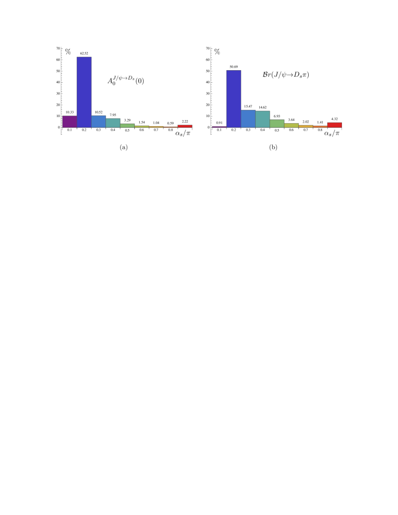
Figure 3: Contributions to form factor $A_{0}^{J/{\psi}{\to}D_{s}}$ in (a) and branching ratio ${\cal B}r(J/{\psi}{\to}D_{s}{\pi})$ in (b) from different regions of ${\alpha}_{s}/{\pi}$ (horizontal axes), where the numbers over the histograms denote the percentages of the corresponding contributions.

(3) It is usually thought that the scale of the $c$ quark mass is not large enough, besides the large mass of final states, maybe the momentum transferred in the $J/{\psi}$ ${\to}$ $D_{s,d}P$ decay is soft rather than hard. One might naturally question the validness of the pQCD approach and the reliability of the perturbative calculation. Hence, it is very necessary to check what percentage of contributions come from the (non)perturbative domain. Taking the $J/{\psi}$ ${\to}$ $D_{s}{\pi}$ decay as an example, contributions to form factor $A_{0}^{J/{\psi}{\to}D_{s}}$ and branching ratio ${\cal B}r(J/{\psi}{\to}D_{s}{\pi})$ from different ${\alpha}_{s}/{\pi}$ regions are plotted in Fig.3. It is easily seen that more than 90% [80%] of the contributions of $A_{0}^{J/{\psi}{\to}D_{s}}$ [${\cal B}r(J/{\psi}{\to}D_{s}{\pi})$] come from ${\alpha}_{s}/{\pi}$ ${\leq}$ 0.4 regions, which implies that the $J/{\psi}$ ${\to}$ $D_{s,d}P$ decays might be computable with the pQCD approach. Additionally, as it is well known that ${\cal B}r(J/{\psi}{\to}D_{s}{\pi})$ ${\propto}$ ${|}A_{0}^{J/{\psi}{\to}D_{s}}{|}^{2}$, however, the probability distribution of ${\cal B}r(J/{\psi}{\to}D_{s}{\pi})$ in Fig.3(b) is different from that of $A_{0}^{J/{\psi}{\to}D_{s}}$ in Fig.3(a). In the bin of ${\alpha}_{s}/{\pi}$ ${\in}$ $[0.1,0.2]$, the percentage in Fig.3(a) is larger than that in Fig.3(b), while the case is reversed in other bins. One of the critical factors is the Wilson coefficients $C_{1,2}$ or $a_{1}$ whose absolute values decrease along with the increase of renormalization scale ${\mu}$. As it is discussed pqcd1 ; pqcd2 ; pqcd3 , a perturbative calculation with the pQCD approach is influenced by many factors, for example, the choice of typical scale $t$, Sudakov factors, models of wave functions, etc., which deserve much attention and further study but are beyond the scope of this paper.

(4) There are many uncertainties on branching ratios, especially from scale $t$ and wave functions ($m_{c}$ and hadronic parameters). In addition, other factors, such as the final state interactions which are usually assumed to be important and necessary for $c$ quark decay, different phenomenological models for wave functions, and so on, are not properly considered here, but deserve massive dedicated study. Our results just provide an order of magnitude estimation on the branching ratio.

IV Summary

The nonleptonic $J/{\psi}$ weak decay is allowable within the standard model. In this paper, we investigated the charm-changing $J/{\psi}$ ${\to}$ $D_{s,d}{\pi}$, $D_{s,d}K$ weak decays with pQCD approach. It is found that the estimated branching ratio for the Cabibbo- and color-favored $J/{\psi}$ ${\to}$ $D_{s}{\pi}$ decay can reach up to ${\cal O}(10^{-10})$, which might be promisingly measurable in future experiments.

Appendix A Building blocks of decay amplitudes

The explicit expressions of building blocks ${\cal A}_{i}$ are collected as follows:

$${\cal A}_{a} = {\int}_{0}^{1}dx_{1}{\int}_{0}^{1}dx_{2}{\int}_{0}^{\infty}b_{1}db_{1}{\int}_{0}^{\infty}b_{2}db_{2}\,{\phi}_{\psi}^{v}(x_{1})\,E_{ab}(t_{a})\,H_{ab}({\alpha},{\beta}_{a},b_{1},b_{2})$$ (42)

$${\times} {\alpha}_{s}(t_{a})\,a_{1}(t_{a})\Big{\{}{\phi}_{D}^{a}(x_{2})\,\Big{[}(t+s)\,\bar{x}_{2}-(t+u)\Big{]}-2\,m_{2}\,m_{c}\,{\phi}_{D}^{p}(x_{2})\Big{\}},$$

$${\cal A}_{b} = {\int}_{0}^{1}dx_{1}{\int}_{0}^{1}dx_{2}{\int}_{0}^{\infty}b_{1}db_{1}{\int}_{0}^{\infty}b_{2}db_{2}\,E_{ab}(t_{b})\,H_{ab}({\alpha},{\beta}_{a},b_{2},b_{1})\,{\alpha}_{s}(t_{b})\,a_{1}(t_{b})$$ (43)

$${\times} \Big{\{}{\phi}_{\psi}^{v}(x_{1})\,{\phi}_{D}^{a}(x_{2})\,\Big{[}(t-s)-(t-u)\,\bar{x}_{1}\Big{]}-{\phi}_{\psi}^{t}(x_{1})\,{\phi}_{D}^{p}(x_{2})\,4\,m_{1}\,m_{2}\,x_{1}\Big{\}},$$

$${\cal A}_{c} = \frac{2}{N_{c}}{\int}_{0}^{1}dx_{1}{\int}_{0}^{1}dx_{2}{\int}_{0}^{1}dx_{3}{\int}_{0}^{\infty}db_{1}{\int}_{0}^{\infty}b_{2}db_{2}{\int}_{0}^{\infty}b_{3}db_{3}$$ (44)

$${\times} {\phi}_{P}^{a}(x_{3})\,E_{cd}(t_{c})\,H_{cd}({\alpha},{\beta}_{c},b_{2},b_{3})\,{\alpha}_{s}(t_{c})\,C_{2}(t_{c})$$

$${\times} \Big{\{}{\phi}_{\psi}^{v}(x_{1})\,{\phi}_{D}^{a}(x_{2})\,\Big{[}t\,(\bar{x}_{1}-\bar{x}_{2})+s\,(\bar{x}_{2}-x_{3})\Big{]}$$

$$+{\phi}_{\psi}^{t}(x_{1})\,{\phi}_{D}^{p}(x_{2})\,m_{1}\,m_{2}\,(\bar{x}_{2}-\bar{x}_{1})\Big{\}}\,{\delta}(b_{1}-b_{2}),$$

$${\cal A}_{d} = \frac{2}{N_{c}}{\int}_{0}^{1}dx_{1}{\int}_{0}^{1}dx_{2}{\int}_{0}^{1}dx_{3}{\int}_{0}^{\infty}db_{1}{\int}_{0}^{\infty}b_{2}db_{2}{\int}_{0}^{\infty}b_{3}db_{3}$$ (45)

$${\times} {\phi}_{P}^{a}(x_{3})\,E_{cd}(t_{d})\,H_{cd}({\alpha},{\beta}_{d},b_{2},b_{3})\,{\alpha}_{s}(t_{d})\,C_{2}(t_{d})$$

$${\times} {\delta}(b_{1}-b_{2})\,\Big{\{}{\phi}_{\psi}^{v}(x_{1})\,{\phi}_{D}^{a}(x_{2})\,s\,(x_{2}-x_{3})$$

$$+{\phi}_{\psi}^{t}(x_{1})\,{\phi}_{D}^{p}(x_{2})\,m_{1}\,m_{2}\,(x_{1}-x_{2})\Big{\}},$$

where $b_{i}$ is the conjugate variable of the transverse momentum $k_{iT}$; ${\alpha}_{s}$ is the QCD running coupling; $a_{1}$ $=$ $C_{1}$ $+$ $C_{2}/N_{c}$.

The hard scattering function $H_{i}$ and Sudakov factor $E_{i}$ are defined as follows.

$$H_{ab}({\alpha},{\beta},b_{i},b_{j})=K_{0}(b_{i}\sqrt{-{\alpha}})\Big{\{}{\theta}(b_{i}-b_{j})K_{0}(b_{i}\sqrt{-{\beta}})I_{0}(b_{j}\sqrt{-{\beta}})+(b_{i}{\leftrightarrow}b_{j})\Big{\}},$$ (46)

$$H_{cd}({\alpha},{\beta},b_{2},b_{3}) = \Big{\{}{\theta}(-{\beta})K_{0}(b_{3}\sqrt{-{\beta}})+\frac{{\pi}}{2}{\theta}({\beta})\Big{[}iJ_{0}(b_{3}\sqrt{{\beta}})-Y_{0}(b_{3}\sqrt{{\beta}})\Big{]}\Big{\}}$$ (47)

$${\times} \Big{\{}{\theta}(b_{2}-b_{3})K_{0}(b_{2}\sqrt{-{\alpha}})I_{0}(b_{3}\sqrt{-{\alpha}})+(b_{2}{\leftrightarrow}b_{3})\Big{\}},$$

$$E_{ab}(t)\ =\ {\exp}\{-S_{\psi}(t)-S_{D}(t)\},$$ (48)

$$E_{cd}(t)\ =\ {\exp}\{-S_{\psi}(t)-S_{D}(t)-S_{P}(t)\},$$ (49)

$$S_{\psi}(t)\ =\ s(x_{1},p_{1}^{+},1/b_{1})+2{\int}_{1/b_{1}}^{t}\frac{d{\mu}}{\mu}{\gamma}_{q},$$ (50)

$$S_{D}(t)\ =\ s(x_{2},p_{2}^{+},1/b_{2})+2{\int}_{1/b_{2}}^{t}\frac{d{\mu}}{\mu}{\gamma}_{q},$$ (51)

$$S_{P}(t)\ =\ s(x_{3},p_{3}^{+},1/b_{3})+s(\bar{x}_{3},p_{3}^{+},1/b_{3})+2{\int}_{1/b_{3}}^{t}\frac{d{\mu}}{\mu}{\gamma}_{q},$$ (52)

where $J_{0}$ and $Y_{0}$ ($I_{0}$ and $K_{0}$) are the (modified) Bessel function of the first and second kind, respectively; the expression of $s(x,Q,1/b)$ can be found in the appendix of Ref.pqcd1 ; ${\gamma}_{q}$ $=$ $-{\alpha}_{s}/{\pi}$ is the quark anomalous dimension; ${\alpha}$ and ${\beta}$ are gluon and quark virtuality, respectively, which are listed as follows.

$${\alpha} = \bar{x}_{1}^{2}m_{1}^{2}+\bar{x}_{2}^{2}m_{2}^{2}-\bar{x}_{1}\bar{x}_{2}t,$$ (53)

$${\beta}_{a} = m_{1}^{2}-m_{c}^{2}+\bar{x}_{2}^{2}m_{2}^{2}-\bar{x}_{2}t,$$ (54)

$${\beta}_{b} = m_{2}^{2}+\bar{x}_{1}^{2}m_{1}^{2}-\bar{x}_{1}t,$$ (55)

$${\beta}_{c} = \bar{x}_{1}^{2}m_{1}^{2}+\bar{x}_{2}^{2}m_{2}^{2}+x_{3}^{2}m_{3}^{2}$$ (56)

$$- \bar{x}_{1}\bar{x}_{2}t-\bar{x}_{1}x_{3}u+\bar{x}_{2}x_{3}s,$$

$${\beta}_{d} = x_{1}^{2}m_{1}^{2}+x_{2}^{2}m_{2}^{2}+x_{3}^{2}m_{3}^{2}$$ (57)

$$- x_{1}x_{2}t-x_{1}x_{3}u+x_{2}x_{3}s,$$

$$t_{a(b)} = {\max}(\sqrt{-{\alpha}},\sqrt{-{\beta}_{a(b)}},1/b_{1},1/b_{2}),$$ (58)

$$t_{c(d)} = {\max}(\sqrt{-{\alpha}},\sqrt{{|}{\beta}_{c(d)}{|}},1/b_{2},1/b_{3}).$$ (59)

References

• (1) J. Aubert et al., Phys. Rev. Lett. 33, 1404 (1974).
• (2) J. Augustin et al., Phys. Rev. Lett. 33, 1406 (1974).
• (3) M. Gell-Mann, Phys. Lett. 8, 214 (1964).
• (4) K. Olive et al. (Particle Data Group), Chin. Phys. C 38, 090001 (2014).
• (5) S. Okubo, Phys. Lett. 5, 165 (1963).
• (6) G. Zweig, CERN-TH-401, 402, 412 (1964).
• (7) J. Iizuka, Prog. Theor. Phys. Suppl. 37-38, 21 (1966).
• (8) H. Li, Phys. Rev. D 52, 3958 (1995).
• (9) C. Chang, H. Li, Phys. Rev. D 55, 5577 (1997).
• (10) T. Yeh, H. Li, Phys. Rev. D 56, 1615 (1997).
• (11) H. Li, S. Zhu, Chin. Phys. C 36, 932 (2012).
• (12) R. Aaij et al. (LHCb Collaboration), Eur. Phys. J. C 71, 1645 (2011).
• (13) M. Ablikim et al. (BESIII Collaboration), Phys. Rev. D 89, 071101 (2014).
• (14) M. Beneke et al., Phys. Rev. Lett. 83, 1914 (1999).
• (15) M. Beneke et al., Nucl. Phys. B 591, 313 (2000).
• (16) M. Beneke et al., Nucl. Phys. B 606, 245 (2001).
• (17) C. Bauer et al., Phys. Rev. D 63, 114020 (2001).
• (18) C. Bauer, D. Pirjol, I. Stewart, Phys. Rev. D 65, 054022 (2002).
• (19) C. Bauer et al., Phys. Rev. D 66, 014017 (2002).
• (20) M. Beneke et al., Nucl. Phys. B 643, 431 (2002).
• (21) R. Verma, A. Kamal and A. Czarnecki, Phys. Lett. B 252, 690 (1990).
• (22) K. Sharma and R. Verma, Int. J. Mod. Phys. A 14, 937 (1999).
• (23) R. Dhir, R. Verma and A. Sharma, Adv. High Energy Phys, 2013, 706543 (2013).
• (24) J. Sun et al., Int. J. Mod. Phys. A 30, 1550094 (2015).
• (25) G. Buchalla, A. Buras, M. Lautenbacher, Rev. Mod. Phys. 68, 1125, (1996).
• (26) L. Wolfenstein, Phys. Rev. Lett. 51, 1945 (1983).
• (27) N. Cabibbo, Phys. Rev. Lett. 10, 531 (1963).
• (28) M. Kobayashi and T. Maskawa, Prog. Theor. Phys. 49, 652 (1973).
• (29) G. Lepage, S. Brodsky, Phys. Rev. D 22, 2157 (1980).
• (30) T. Kurimoto, H. Li, A. Sanda, Phys. Rev. D 65, 014007 (2001).
• (31) P. Ball, V. Braun, A. Lenz, JHEP, 0605, 004, (2006).
• (32) G. Lepage et al., Phys. Rev. D 46, 4052 (1992).
• (33) G. Bodwin, E. Braaten, G. Lepage, Phys. Rev. D 51, 1125 (1995).
• (34) N. Brambilla et al., Rev. Mod. Phys. 77, 1423 (2005).
• (35) B. Xiao, X. Qin, B. Ma, Eur. Phys. J. A 15, 523 (2002).
• (36) E. Eichten and C. Quigg, Phys. Rev. D 52, 1726 (1995).
• (37) R. Li, C. LΓΌ, H. Zou, Phys. Rev. D 78, 014018 (2008).
• (38) M. Wirbel, B. Stech and M. Bauer, Z. Phys. C 29, 637 (1985).
• (39) A. Kamal, Particle Physics, Springer, 2014, p. 298.
• (40) Y. Wang et al., Eur. Phys. J. C 55, 607 (2008).