Compactons and their variational properties for degenerate KdV and NLS in dimension 1
Abstract.
We analyze the stationary and traveling wave solutions to a family of degenerate dispersive equations of KdV and NLS-type. In stark contrast to the standard soliton solutions for non-degenerate KdV and NLS equations, the degeneracy of the elliptic operators studied here allows for compactly supported steady or traveling states. As we work in dimension, ODE methods apply, however the models considered have formally conserved Hamiltonian, Mass and Momentum functionals, which allow for variational analysis as well.
1. Introduction
1.1. The classical theory
Before discussing the degenerate models that will be the focus of this article, it is good to have in mind the basic properties of the canonical one-dimensional models; classical references are [37, 38], see [2] for ground states of more general semilinear one-dimensional models.
Consider the Hamiltonian (defined on functions on the real line)
The associated Hamiltonian flows through the symplectic forms and are, respectively, the generalized Korteweg-de Vries and nonlinear Schrödinger equations
| (KdV) | |||
| (NLS) |
The profile of traveling waves of (KdV) of the form , or of stationary waves of (NLS) of the form solves
The only localized (decaying at infinity) solution of this equation is, up to translations,
Both (KdV) and (NLS) conserve the -mass of the solution, and the above solutions can be viewed as critical points of the Hamiltonian under the constraint that the -mass is fixed to some value. These critical points are actually global minimizers in the -subcritical case , which leads to the orbital stability of these stationary waves.
Making use of the pseudo-Galilean invariance gives translating solutions of the nonlinear Schrödinger equation of the form ; they can also be characterized as minimizers of the Hamiltonian for fixed mass and momentum.
1.2. A Hamiltonian leading to degenerate dispersion
The aim of the present paper is to examine the situation if the Hamiltonian becomes
making the equation quasilinear and degenerate close to . We will assume throughout that
We will see that a number of interesting phenomena occur:
-
•
Decaying stationary waves become compactly supported instead of exponentially decaying.
-
•
The family of stationary waves becomes two-dimensional (up to translations) instead of one-dimensional.
-
•
Out of these stationary waves, some, but not all, are energy minimizing for fixed mass.
-
•
The pseudo-Galilean symmetry has to be modified in a nonlinear way.
The degenerate KdV and NLS equations, obtained through the symplectic forms and respectively, read
| (dKdV) | ||||
| (dNLS) |
(where is real-valued for (dKdV) and complex-valued for (dNLS)). Both equations conserve the mass
and additional conservation laws are given by
Degenerate KdV-type equations were first introduced and studied by Rosenau and Hyman [32, 31]; their primary interest was the existence of compactons. A Hamiltonian version of the Rosenau-Hyman equations was then proposed by Cooper, Shepard and Sodano [11, 27]; a particular case of this family of equations is given by (dKdV). A Schrödinger version of the Rosenau-Hyman equations was proposed in [43], of which (dNLS) is a particular case.
The equations (dKdV) and (dNLS) are perhaps the simplest instances of degenerate dispersion; more elaborate models involving degenerate dispersion occur in the description of a variety of physical phenomena: to cite a few [3, 36, 29, 8, 19, 12, 4]. It is our hope that the analysis of the model equations (dKdV) and (dNLS) will be an interesting step in the development of the mathematical theory of degenerate nonlinear dispersive equations, which remains very primitive.
1.3. Obtained results
1.3.1. Compactons for (dKdV)
Traveling waves of (dKdV) are given by the ansatz and satisfy the ODE
The analysis of this ODE leads in particular to the following theorem:
Theorem 1.1.
For and , or and , there exist compactons solving the above ODE (in the sense of distributions) which are even, compactly supported on , decreasing on , and satisfy
These compactons can be combined to yield multi-compacton solutions
where , and the have non overlapping supports.
This theorem is proved in Section 2.
1.3.2. Variational properties
A classical idea to generate traveling waves is to consider the minimizing problem
where is a fixed, positive constant. Traveling waves obtained through this minimization procedure are orbitally stable (as long as the flow around them can be defined).
Theorem 1.2.
For , the above minimization problem admits a minimizer, which is (up to translation) one of the . For , the minimizer is with .
Remark 1.3.
While the proof of the above theorem relies on a concentration compactness result, we learned from Rupert Frank of the reference [28], where Sz. Nagy derives the same result from a very clever use of elementary inequalities. Sz. Nagy is also able to identify the minimizers as for any .
1.3.3. Compactons for (dNLS)
Traveling waves of (dNLS) are given by the ansatz ; they satisfy the equation
Theorem 1.4.
For and , or and , there exist compactons satisfying the above ODE. They are given by
where
This theorem is proved in Section 3.
1.3.4. The linearized problem for (dKdV)
Linearizing (dKdV) around one of the compacton traveling waves results in the equation
(in the moving frame). This equation has to be supplemented with appropriate boundary conditions.
We discuss in Section 4, in the case ,
-
•
The spectrum of the operators , which depends on the compacton considered
-
•
A local well-posedness theory for the linearized evolution problem above.
1.3.5. Numerical results
Numerical results on the traveling waves and their stability are given in Section 5.
2. Solitary waves for (dKdV)
2.1. The ODE
By definition, traveling waves at velocity are solutions of the form
Inserting this ansatz in the equation leads to
| (2.1) |
This is equivalent to
| (2.2) |
for an integration constant . Multiplying by , we get for a new integration constant
or equivalently
| (2.3) |
The following proposition classifies solutions of this ODE:
Proposition 2.1.
Assume . We will denote be the unique positive solution of , when it exists.
Consider a solution of (2.1), with speed and integration constants and , which is positive over the (maximal) interval . Up to translation, there are three possibilities
-
(i)
, and the solution is periodic. Such a solution exists in particular if , or and , and, if exists, .
-
(ii)
. This is the case if and only exists, satisfies ; if furthermore is positive on ; and if finally , or and , or and . Then
and the behavior of for is as in the following point.
-
(iii)
for some , and the solution is even. This is the case if and only if one of the two following conditions is satisfied:
-
(1)
and , or and , and furthermore if exists. Then, as ,
-
(2)
and , or , . Then, as ,
-
(1)
Remark 2.2.
The case behaves differently from , and has therefore not been included in the above. We refer to Section 2.3 for a description of compactons in this case.
Proof.
Recall that, once the integration constants are fixed, satisfies . Thus, for , and fixed, we think of the phase space as foliated by sets of the type .
If the set is bounded, we are in the situation of .
If it is unbounded, we are either in the situation , or . Situation corresponds to the case where the stable point satisfies . Notice that for , exists for , and satisfies then . Then
Simply comparing signs, we see that the above inequality cannot hold for , so that for , .
In order to establish the behavior close to in the case , (the other cases being similar), we need to integrate locally the ODE
Expanding , we obtain that
from which we deduce the desired expansion
We next consider the point at which vanishes first. If this point is also a stationary point of the phase portrait, i.e. , then we are in case . Otherwise, we can prolong the solution by symmetry to obtain case . ∎
2.2. The compactons
We will mostly focus on finite mass (or, equivalently, finite energy) traveling waves. We will denote for the maximal positive solution corresponding to in Proposition 2.1 with , , and ; or , and , prolonged by outside of its domain of positivity, which we denote . Recapitulating,
-
•
even.
-
•
and smooth on .
-
•
on .
-
•
decreasing on .
Let us check that satisfies (2.1) in the sense of distributions on . This is implied by the equality
in the sense of distributions. The only delicate points are of course ; more precisely, it is easy to see that is the sum of a bounded function and of . But since vanishes at , the product is a bounded function; from there it is easy to check that the above holds.
Notice that, defining in a similar way to , it does not satisfy (2.1) in the sense of distributions on but rather
This leads to the following proposition:
Corollary 2.3.
For a velocity , general solutions of finite mass of (2.1) (in the sense of distributions) are of the form
where , either or , , and the supports of the are disjoint.
2.3. Explicit formulas
If , , the equation (2.2) becomes
| (2.4) |
Setting , this becomes
| (2.5) |
Assuming that is even, this can be integrated to give that , where . This gives the compacton
If , , the equation for becomes linear:
It can easily be integrated to yield that with , which leads to three cases:
-
•
If and , then periodic solutions are given by
-
•
If and , then compactons are given by
(2.6) where is the least positive solution of .
-
•
If and , a compacton is given by
2.4. The energy and mass of compactons
Notice first the scaling property: for any ,
Next, we record how the Hamiltonian, Mass, and support of are related:
Proposition 2.4.
The compacton satisfies
Proof.
The desired formula follows by combining the energy identity
which can be obtained by multiplying (2.2) with by , and integrating by parts, making sure that the boundary terms vanish, with the Pohozaev identity
(which can be obtained by multiplying (2.2) with by , and integrating; or equivalently, by integrating over ).
∎
Proposition 2.5.
If , the minimum of given is reached for and . The value of the minimum is .
Proof.
From Proposition (2.4), we learn if that
This implies first that the minimum of is reached for , which we assume from now on; equivalently, . Next, since is fixed at , the above becomes
Thus our aim becomes: find the the compacton with mass and the largest speed . An easy computation using the formula (2.6) gives
Since the function is decreasing on , we find that the largest value of is reached when , or equivalently . ∎
Proposition 2.6.
If , there is no compacton which achieves the minimum of for fixed.
Proof.
A simple computation gives that
so that the infimum is achieved for ; but is not allowed for the compactons . ∎
2.5. Variational analysis for
Theorem 2.7 (Ground state).
If , then for any , , and this variational problem admits minimizers. Modulo translation, they are of the form with .
If , the minimizing compacton is
Remark 2.8.
It is probably the case that the minimizer is given by for any .
Proof.
Switching to the unknown function , the problem becomes that of minimizing
The Gagliardo-Nirenberg inequality
| (2.7) |
implies that
Furthermore, since, for any , , and any , we have while
Finally, observe the scaling law:
It suffices to show the existence of a minimizer for , so we consider a minimizing sequence for such that , . We now apply the following concentration compactness result
Proposition 2.9.
Consider a bounded sequence of nonnegative functions in . Then there exists a subsequence (still denoted ), a family of sequences , and functions such that, defining furthermore by
there holds
-
•
, as ;
-
•
, and ;
-
•
as for all ;
-
•
as ;
-
•
as for all .
The proof follows mutatis mutandis from the proof of Proposition 3.1. in [15] after the definition of has been changed to .
We apply this proposition to the minimizing sequence , implying first that
Letting first , and then , the above proposition implies that
Denoting , the above proposition gives that . Using the definition of , its scaling, its negativity, and convexity, the last inequality implies that
All the inequality signs above have to be equality signs; but this is only possible if (up to relabeling) while for . Then is the desired minimizer!
Since , it is continuous. Consider an interval where it is positive, choose , and let . Since and , we obtain that satisfies
for a Lagrange multiplier which might depend on . Coming back to , this implies that
where , , , and the are such that the supports of the are disjoint. Letting , we have . But then
Once again, this implies that all but one of the are zero, or in other words,
If , we learn from Proposition 2.5 that the minimizing compacton is such that . ∎
2.6. Variational analysis for
When , we must deal with the lack of compactness that occurs when traditionally trying to minimize energy with respect to fixed mass. One approach to this is to use the so-called Weinstein functional as introduced in [42].
For simplicity, take to start. In such a case, the optimization procedure is to maximize a functional built from the Gagliardo-Nirenberg inequality (2.7). The functional is of the form
| (2.8) |
with , . The existence proof works nearly identically to the existence arguments in [42] via scaling arguments with the appropriately modified scalings to deal with the degenerate -type norm. For , a similar strategy will work provided one correctly modifies the powers in Gagliardo-Nirenberg inequality from (2.7) to give
| (2.9) |
for and . We remark here that in a similar fashion the best constant in the Galgliardo-Nirenberg inequality (2.7) is given by a function of the norm of the ground state solution for each .
One could also propose an alternative constrained minimization given by finding the minimizer of
| (2.10) |
such that
| (2.11) |
Solutions of this minimization can be seen to solve the correct ODE equation after a suitable scaling argument is applied. For a fairly general treatment of these strategies in a general framework for semilinear operators, see for instance [9].
3. Solitary waves for (dNLS)
3.1. The ODE
By definition, traveling waves are solutions of the form
with . They satisfy the equation
| (3.1) |
For , a first class of solutions is obviously given by , defined in the previous section. Our aim, however, is to completely describe finite mass solutions. This is achieved in the following theorem
Theorem 3.1.
Proof.
A computation shows that the are indeed solutions in the sense of distributions. We now prove that they are the only ones.
Multiplying (3.1) by and taking the imaginary part, or multiplying the equation by and taking the real part leads to the identities
Therefore, there exist real constants and such that, as long as does not vanish,
| (3.3a) | ||||
| (3.3b) | ||||
If the traveling wave is to have finite mass, then necessarily as approaches some (which might be infinite). Letting , we learn from (3.3b) that is bounded. Turning to (3.3a), we learn that
To pursue the discussion, we split it into two cases
Case 1: . If , equation (3.3a) implies that . This in turn means that has a constant phase, so that we can assume, using the symmetries of the equation, that is real valued. It solves
which brings us back to the previous section.
3.2. Variational properties
It is clear that the results in Section 2.5 extend to the case of complex-valued functions: namely, the complex-valued minimizers of subject to constant coincide with the real-valued minimizers.
In analogy with the semilinear case, it would be natural to expect that the appear as the minimizers of
but we will see it is not the case. Adopting the polar decomposition , this becomes.
A non-compact minimizing sequence can be constructed as follows: consider in be radial, with support , , and let . Next, let solve . Finally, let be a minimizer of subject to and define
so that most of the mass and the energy lies in the first summand, while all the momentum is contained in the second, non compact, summand. To be more precise, a small computation reveals that
Letting and choosing for instance gives a minimizing sequence such that
Due to (3.2), this example shows that cannot be minimizers; it also illustrates the basic lack of compactness which explains the absence of minimizers.
3.3. Hydrodynamic formulation
The existence of traveling waves for (dNLS) can be read off most easily after switching to hydrodynamic coordinates: taking the Madelung transform leads to the equation
Defining as the designated flow velocity, the equation becomes
| (3.4) | ||||
Traveling waves now correspond to solutions of
which provides an alternative (and, in some respects, simpler) proof of the results of Subsection 3.1.
This can be contrasted with a related model derived by John Hunter [17, Section ] that arises as an asymptotic equation for a two-wave system in a compressible gas dynamics put forward by Majda-Rosales-Schonbek [22]. The degenerate NLS model is given by
| (3.5) |
This equation was introduced to the authors during a talk of John Hunter and is now being studied in significant detail by Hunter and graduate student Evan Smothers [18].
Naively taking the Madelung transformation of (3.5), , for this equation, we arrive at
for . The right hand side of the equation no longer quite so clearly supports coherent structures, but might be ideal for the study of shock-like solutions. It is unclear however whether the variational approach which we used for (dNLS) will yield useful results.
Remark 3.2.
One might also from Euler systems of this type attempt to derive a weakly dispersive KdV limit as in the study of dispersive shock waves a la Whitham theory. See for instance the review article of El-Hoefer-Shearer [13].
4. Linear Stability for Compactons of (dKdV) when
In this section, we study the operator stemming from linearizing (dKdV) with about solutions
both when and . When , but , a similar analysis should follow. However as is both the power in the original derivation and the most interesting algebraically, we focus on it primarily here. For simplicity of exposition, we will treat the following specific cases:
-
(1)
, ;
-
(2)
:
-
(a)
;
-
(b)
;
-
(c)
,
-
(a)
though other values of and appropriately related follow with small modifications.
We assume that our initial data is of the form
where the perturbation is sufficiently small, smooth and . For times we assume that our solution may be written in the form
In the moving frame, keeping only the linear terms in we obtain the equation
| (4.1) |
where linearized operator,
| (4.2) |
can be seen as a singular Sturm-Liouville operator and written in the form
Remark 4.1.
In order to better characterize the behavior of the eigenfunctions of we recall the Sturm comparison and oscillation theorems (see for example [40, Theorems 9.39, 9.40]):
Theorem 4.2 (Sturm comparison).
Let and be solutions to the ODE
on some open interval . Suppose that at each endpoint either or if the endpoint lies in the interior of the interval we have . Then the function has a zero in the interval .
Remark 4.3.
From standard ODE theory are smooth on the open interval and hence the Wronskian is well defined on . If then we define
provided such a limit exists. A similar definition holds when . A consequence of being limit point is that for all eigenfunctions of this limit exists and is equal to zero,
Theorem 4.4 (Sturm oscillation).
If has eigenvalues with corresponding eigenfunctions then has exactly zeros in the interval .
We consider to be a symmetric unbounded operator on with domain . For we may integrate by parts to obtain
We may then associate with the corresponding Friedrichs extension.
4.1. The case ,
We first consider the setting , where we recall the explicit expression
We then have the following properties of the operator :
Proposition 4.5.
The operator is limit point and satisfies the following:
-
(1)
The ground state energy is with positive ground state .
-
(2)
The first excited eigenvalue is with corresponding eigenfunction .
-
(3)
The operator has continuous spectrum .
First, let us observe that is limit point. Indeed, is equivalent, upon setting , to . Therefore, the general solution reads ; for , , this solution is not square integrable at either endpoint so by the Weyl alternative the operator is limit point at and the Friedrichs extension is the unique self-adjoint extension of (see for example [40, Theorems 9.6, 9.9]).
Under the (invertible) transformation
| (4.3) |
we can translate the operator to standard elliptic problem on all of . To see this, we will reformulate (4.2) as a simple -operator on . This is the strategy of the standard -calculus as developed by Melrose and many others, see e.g. [24, 25, 23, 26, 14].
We easily observe that we have
and as a result
where
From the asymptotics of near , we recognize that as . Conjugating by the integrating factor
we arrive at the simple elliptic operator
| (4.4) |
which must then have the same spectrum as the operator .
The operator is thus seen to be a relatively compact perturbation of and hence by Weyl’s Theorem has continuous spectrum . With regards to the discrete spectrum, note that and is a nice function in the variables, in fact, it is exponentially decaying. Plugging in , we observe that has a negative eigenvalue at . We also have , which turns into an eigenvalue for also at given that is exponentially decaying as . By Sturm oscillation theory for elliptic operators, we can see that there are no eigenvalues between and .
This is sufficient to set up elliptic estimates for and do the finite time modulation theory proposed in this work. For future work on long and/or global time scales, it is important to understand dispersive estimates for the linearized operator. In such a case, we will need to potentially rule out a resonance at the endpoint of the continuous spectrum , see [33].
4.1.1. Spectral Theory without the Nonlinear Transformation
It is possible to determine the spectrum without changing coordinates: first notice that, due to the ODE satisfied by ,
Since vanishes once on , we deduce, by the Sturm oscillation theorem [40], that is the first excited mode.
To determine the behavior at the endpoints of I of a solution of , which can also be written
We now apply Frobenius’ method [39]. Since both endpoints are symmetrical, it suffices to consider the left endpoint . Switching variable to , observe that . Only the top orders of the expansion of the coefficients matters for Frobenius’ method, so that we can consider the equation
The indicial equation (obtained by plugging in the above) reads , leading to the characteristic exponents
Frobenius’ method gives a basis of solutions behaving as . Observe that this leads to an infinite number of oscillations for . Thus, the continuous spectrum is , see [41, Page 220].
4.1.2. The solution operator for in general for ,
A calculation shows that linearly independent solutions to now correspond to and . The function since as . The function in either direction. Note, the modified Wronskian satisfies
| (4.5) |
If , the general solution is given by
| (4.6) | ||||
where .
To construct a semigroup for below for , , we need that is a reasonable operator where
We thus collect the following result:
Lemma 4.6.
The operator is continuous where
Proof.
This follows immediately from the spectral theory above. In particular, is bounded away from from below on , meaning that is a bounded operator on this space and hence continuous.
One can also prove this using directly the form of (4.6). ∎
4.2. The case
We now turn to the case and recall the explicit expression,
We summarize the properties of the operator as follows:
Proposition 4.7.
For the operator satisfies the following:
-
(1)
The operator limit point at
-
(2)
The operator has discrete spectrum and there exists an orthogonal basis of consisting of simple eigenfunctions of .
-
(3)
The ground state is given by with corresponding ground state energy .
-
(4)
The first eigenvalue is positive.
4.2.1. The operator is limit point
To show the operator is limit point we observe as before that the general solution to the homogeneous equation is given by .
When we may take , , to obtain two linearly independent solutions to given by
| (4.7) |
that satisfy the boundary conditions
As the length of the interval we have
so the operator is limit point.
When we have . However, we may construct a second solution to the homogeneous ODE by taking
and note that the operator is still limit point as .
4.2.2. The operator is Hilbert-Schmidt
We now consider solutions to the ODE
| (4.8) |
If and , the unique solution is given by
| (4.9) |
where the constant is given by the (modified) Wronskian of the functions ,
Using the formula (4.9), we may then show that operator extends to a compact operator on :
Lemma 4.8.
If the operator extends to a Hilbert-Schmidt operator on . In particular, the operator has discrete spectrum and there exists a basis of consisting of simple eigenfunctions of .
Proof.
The kernel of the operator is given by
Taking we may use the fact that near and the explicit expression (4.7) to obtain the bounds
In particular,
and hence
Integrating this in we see that the operator is Hilbert-Schmidt and hence compact. The fact that the eigenvalues of are simple follows from the fact that is limit point at . ∎
When we require an orthogonality condition to obtain a unique solution to the ODE (4.8). Thus we define the space
For satisfying we take to be the unique solution to the equation (4.8) given by
| (4.10) | ||||
An essentially identical proof to Lemma 4.8 yields the following:
Lemma 4.9.
If the operator extends to a Hilbert-Schmidt operator on the space . In particular, the operator has discrete spectrum and there exists a basis of consisting of simple eigenfunctions of .
4.2.3. The ground state and first harmonic
Recalling that has no zeros in the interval we see that this is the ground state. In particular, for we must have that the first harmonic has positive eigenvalue . In the case we have the following lemma:
Lemma 4.10.
When the first eigenvalue is positive.
Proof.
Suppose for a contradiction that . Let be the zero of the corresponding eigenfunction and, recalling that the length of the interval , we must either have or . Without loss of generality assume that . If lies in the domain of , then we must have that so recalling the Wronskian is given by
we see that . In particular, taking we may apply the Sturm comparison principle on the interval to show that must have a zero in the interval , which is a contradiction. Thus, . ∎
4.3. Energy spaces
The equation (4.1) has a formally conserved energy,
From Propositions 4.5, 4.7 we see that
and hence we may define a natural energy space associated to the equation (4.1) given by the completion of under the norm
As the -norm is not conserved by (4.1) it is natural to define the subset where we define
where we note that the orthogonality condition
is conserved by the flow of (4.1) for all choices of and that the orthogonality condition
is conserved when due to the fact that . A simple consequence of Propositions 4.5, 4.7 is that whenever we have the estimate
| (4.11) |
thus it is natural to define the norm
with associated inner product
We now consider the operator as an unbounded operator on with domain
We may endow with the norm
and then have the following lemma:
Lemma 4.11.
The embedding is compact.
Proof.
If then we may use the fact that and the estimate (4.11) to obtain
where is the usual Sobolev space on .
Now let be a bounded sequence. Then is also bounded so as the embedding is compact, passing to a subsequence there exists some so that
Next we define (or when or ) and by continuity of ,
Finally we observe that if and ,
where the integration by parts may be justified by observing that whenever we have and hence . Taking in this identity we then obtain
as required. ∎
4.4. The linear semigroup and local well-posedness of a linear equation
For all we have
| (4.12) |
and hence is dissipative. This then allows us to construct a semigroup :
Lemma 4.12.
The operator generates a contraction semigroup .
Proof.
It suffices to show that . By construction the inverse operator is well-defined. From Lemma 4.11 the embedding is compact and hence is a compact operator on . From the estimate (4.12) there does not exist a non-trivial solution to the homogeneous equation
so applying the Fredholm alternative to the operator we see that as required. ∎
We note that using the semigroup we may construct a mild solution to the linear equation
| (4.13) |
whenever and using the Duhamel formula
Further, the solution satisfies the energy estimate
where
This construction may then be straightforwardly extended to handle initial data in the energy space using a simple modulation argument.
Remark 4.13.
We remark that the solution to (4.13) does not quite extend to a solution to the linearized equation on in the sense of distributions. Indeed, if we take to be extension by zero, then taking and , as distributions on we obtain
4.5. The operators for Linearized (dNLS)
When , a somewhat tedious calculation reveals that linearizing about in the case of degenerate NLS results in an operator of the form
| (4.14) |
when acting on a perturbation , where is as above. Acting on , we have
| (4.15) |
When , the complexity of the phase in makes thing somewhat more complicated. In particular, taking with , we have the linearized equation for the system as
| (4.16) |
The underlying structure of these matrix non-self-adjoint will be a topic for future work, but results analogous to those in the works of for instance Schlag et al should be possible [30, 6, 20, 34, 35].
5. Some Numerical Analysis of the degenerate NLS and KDV equations
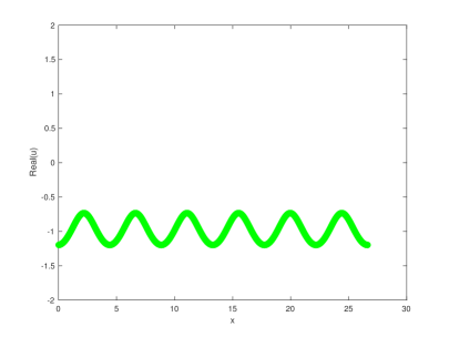
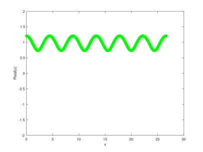
We consider a variation on (dNLS) with , which comes from [10]. In particular, we want to study compacton solutions for
| (5.1) |
Here we use viscosity-type methods as motivated by the work [1], but for prior numerical works on these types of models, see works such as the use of Pade Approximants from Mihaila-Cardenas-Cooper-Saxena [27] and Rosenau-Hyman [32].
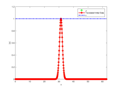
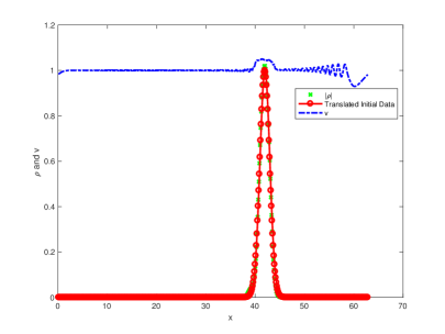
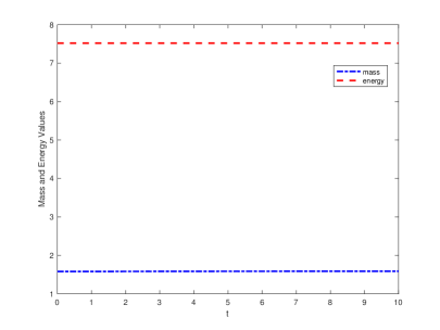
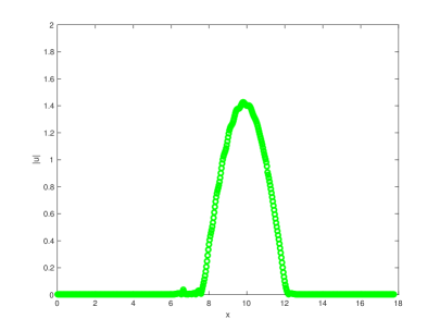
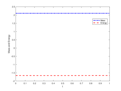
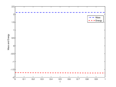
The stability of stationary solutions can be studied numerically in this equation for now in limited cases. To handle all the cases for which we have derived solutions above, more sophisticated numerical tools will need to be developed. Here, we treat only non-degenerate periodic solutions (when or , ) where the degeneracy of the elliptic operator does not arise generally. However, our methods of direct numerical simulation are relatively sensitive, hence for compactons we cannot treat the cases due to the strongly singular phase involved in generating traveling waves in the NLS setting. To discretize (5.1) in the non-degenerate case, motivated by the schemes used to solve degenerate equations in [21], we use a simple centered finite difference scheme with periodic boundary conditions. Once we have generated the finite difference spatial operator for (5.1), we integrate in time using the stiff solver ode15s in Matlab. The results are reported in Figure 3.

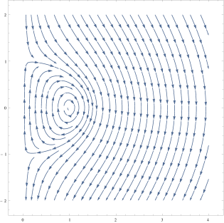
As an alternative, naively taking the Madelung transformation of (5.1), , for this equation, we arrive at
| (5.2) | |||
| (5.3) |
Defining as the designated flow velocity, we have
| (5.4) | ||||
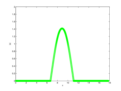
We can numerically solve (5.4) to observe transport with relative ease by using a standard centered finite difference approximation and stiff numerical time integration schemes in Matlab. The results are reported in Figure 4.
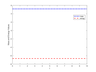
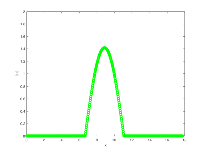
We consider a variation on (dKdV) with
| (5.5) |
which has been proposed and studied in the work of Cooper-Shepard-Sodano [11]. Similar style degenerate dispersion operators have been developed by for instance Hunter-Saxon [19], etc. To discretize (5.1), motivated by the schemes used in [1], we use a pseudospectral scheme with regularized derivatives of the form
| (5.6) |
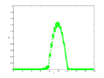
for chosen sufficiently small (generally unless otherwise stated). Once we have generated the regularized pseudospectral spatial operator for (5.1), we integrate in time using the stiff solver ode15s in Matlab. The results are reported in Figures 5 and 6.
References
- [1] D. M. Ambrose, G. Simpson, J. D. Wright, and D. G. Yang. Ill-posedness of degenerate dispersive equations. Nonlinearity, 25(9):2655–2680, 2012.
- [2] H. Berestycki and P.-L. Lions. Nonlinear scalar field equations. I. Existence of a ground state. Arch. Rational Mech. Anal., 82(4):313–345, 1983.
- [3] F. Betancourt, R. Bürger, K. H. Karlsen, and E. M. Tory. On nonlocal conservation laws modelling sedimentation. Nonlinearity, 24(3):855–885, 2011.
- [4] J. Biello and J. K. Hunter. Nonlinear Hamiltonian waves with constant frequency and surface waves on vorticity discontinuities. Comm. Pure Appl. Math., 63(3):303–336, 2010.
- [5] J. L. Bona, S. M. Sun, and B.-Y. Zhang. A nonhomogeneous boundary-value problem for the Korteweg-de Vries equation posed on a finite domain. Comm. Partial Differential Equations, 28(7-8):1391–1436, 2003.
- [6] M. Burak Erdoĝan and W. Schlag. Dispersive estimates for schrödinger operators in the presence of a resonance and/or an eigenvalue at zero energy in dimension three: Ii. Journal d’Analyse Mathématique, 99(1):199–248, 2006.
- [7] M. A. Caicedo and B.-Y. Zhang. Well-posedness of a nonlinear boundary value problem for the Korteweg–de Vries equation on a bounded domain. J. Math. Anal. Appl., 448(2):797–814, 2017.
- [8] R. Camassa and D. D. Holm. An integrable shallow water equation with peaked solitons. Phys. Rev. Lett., 71(11):1661–1664, 1993.
- [9] H. Christianson, J. Marzuola, J. Metcalfe, and M. Taylor. Nonlinear bound states on weakly homogeneous spaces. Communications in Partial Differential Equations, 39(1):34–97, 2014.
- [10] J. E. Colliander, J. L. Marzuola, T. Oh, and G. Simpson. Behavior of a model dynamical system with applications to weak turbulence. Experimental Mathematics, 22(3):250–264, 2013.
- [11] F. Cooper, H. Shepard, and P. Sodano. Solitary waves in a class of generalized Korteweg-de Vries equations. Phys. Rev. E (3), 48(5):4027–4032, 1993.
- [12] H.-H. Dai and Y. Huo. Solitary shock waves and other travelling waves in a general compressible hyperelastic rod. R. Soc. Lond. Proc. Ser. A Math. Phys. Eng. Sci., 456(1994):331–363, 2000.
- [13] G. El, M. Hoefer, and M. Shearer. Dispersive and diffusive-dispersive shock waves for nonconvex conservation laws. SIAM Review, 59(1):3–61, 2017.
- [14] D. Grieser. Basics of the b-calculus. In Approaches to singular analysis, pages 30–84. Springer, 2001.
- [15] T. Hmidi and S. Keraani. Blowup theory for the critical nonlinear Schrödinger equations revisited. Int. Math. Res. Not., (46):2815–2828, 2005.
- [16] J. Holmer. The initial-boundary value problem for the Korteweg-de Vries equation. Comm. Partial Differential Equations, 31(7-9):1151–1190, 2006.
- [17] J. K. Hunter. Asymptotic equations for nonlinear hyperbolic waves. In Surveys in applied mathematics, pages 167–276. Springer, 1995.
- [18] J. K. Hunter. Private communication. 2016.
- [19] J. K. Hunter and R. Saxton. Dynamics of director fields. SIAM J. Appl. Math., 51(6):1498–1521, 1991.
- [20] J. Krieger and W. Schlag. Stable manifolds for all monic supercritical focusing nonlinear schrödinger equations in one dimension. Journal of the American Mathematical Society, 19(4):815–920, 2006.
- [21] J.-G. Liu, J. Lu, D. Margetis, and J. L. Marzuola. Asymmetry in crystal facet dynamics of homoepitaxy by a continuum model. arXiv preprint arXiv:1704.01554, 2017.
- [22] A. Majda, R. Rosales, and M. Schonbek. A canonical system of lntegrodifferential equations arising in resonant nonlinear acoustics. Studies in Applied Mathematics, 79(3):205–262, 1988.
- [23] R. Mazzeo. Elliptic theory of differential edge operators i. Communications in Partial Differential Equations, 16(10):1615–1664, 1991.
- [24] R. B. Melrose. Pseudodifferential operators, corners and singular limits. American Mathematical Society, 1990.
- [25] R. B. Melrose. The Atiyah-Patodi-singer index theorem, volume 4. Citeseer, 1993.
- [26] R. B. Melrose. Differential analysis on manifolds with corners, 1996.
- [27] B. Mihaila, A. Cardenas, F. Cooper, and A. Saxena. Stability and dynamical properties of Cooper-Shepard-Sodano compactons. Phys. Rev. E (3), 82(6):066702, 11, 2010.
- [28] B. v. S. Nagy. Über integralungleichungen zwischen einer funktion und ihrer ableitung. Acta Univ. Szeged. Sect. Sci. Math, 10:64–74, 1941.
- [29] V. Nesterenko. Dynamics of heterogeneous materials. 2001.
- [30] I. Rodnianski, W. Schlag, and A. Soffer. Dispersive analysis of charge transfer models. Communications on pure and applied mathematics, 58(2):149–216, 2005.
- [31] P. Rosenau. Nonlinear dispersion and compact structures. Phys. Rev. Lett., 73(13):1737–1741, 1994.
- [32] P. Rosenau and J. M. Hyman. Compactons: solitons with finite wavelength. Physical Review Letters, 70(5):564, 1993.
- [33] W. Schlag. Dispersive estimates for schrödinger operators: a survey. Mathematical aspects of nonlinear dispersive equations, 163:255–285, 2007.
- [34] W. Schlag. Dispersive estimates for schrödinger operators: a survey. Mathematical aspects of nonlinear dispersive equations, 163:255–285, 2007.
- [35] W. Schlag. Stable manifolds for an orbitally unstable nonlinear schrödinger equation. Annals of mathematics, 169(1):139–227, 2009.
- [36] G. Simpson, M. Spiegelman, and M. I. Weinstein. Degenerate dispersive equations arising in the study of magma dynamics. Nonlinearity, 20(1):21–49, 2007.
- [37] C. Sulem and P.-L. Sulem. The nonlinear Schrödinger equation, volume 139 of Applied Mathematical Sciences. Springer-Verlag, New York, 1999. Self-focusing and wave collapse.
- [38] T. Tao. Nonlinear dispersive equations, volume 106 of CBMS Regional Conference Series in Mathematics. Published for the Conference Board of the Mathematical Sciences, Washington, DC; by the American Mathematical Society, Providence, RI, 2006. Local and global analysis.
- [39] G. Teschl. Ordinary differential equations and dynamical systems, volume 140 of Graduate Studies in Mathematics. American Mathematical Society, Providence, RI, 2012.
- [40] G. Teschl. Mathematical methods in quantum mechanics, volume 157 of Graduate Studies in Mathematics. American Mathematical Society, Providence, RI, second edition, 2014. With applications to Schrödinger operators.
- [41] J. Weidmann. Spectral theory of ordinary differential operators, volume 1258. Springer, 2006.
- [42] M. I. Weinstein. Nonlinear schrödinger equations and sharp interpolation estimates. Communications in Mathematical Physics, 87(4):567–576, 1983.
- [43] L. Zhang and L.-Q. Chen. Envelope compacton and solitary pattern solutions of a generalized nonlinear Schrödinger equation. Nonlinear Anal., 70(1):492–496, 2009.