Conley pairs in geometry – Lusternik-Schnirelmann theory and more

Abstract

Firstly, we wish to motivate that Conley pairs, realized via Salamon’s definition [17], are rather useful building blocks in geometry: Initially we met Conley pairs in an attempt to construct Morse filtrations of free loop spaces [21]. From this fell off quite naturally, firstly, an alternative proof [20] of the cell attachment theorem in Morse theory [13] and, secondly, some ideas [12] how to try to organize the closures of the unstable manifolds of a Morse-Smale gradient flow as a CW decomposition of the underlying manifold. Relaxing non-degeneracy of critical points to isolatedness we use these Conley pairs to implement the gradient flow proof of the Lusternik-Schnirelmann Theorem [10] proposed in Bott’s survey [3].

Secondly, we shall use this opportunity to provide an exposition of Lusternik-Schnirelmann (LS) theory based on thickenings of unstable manifolds via Conley pairs. We shall cover the Lusternik-Schnirelmann Theorem [10], cuplength, subordination, the LS refined minimax principle, and a variant of the LS category called ambient category.

1 Introduction and applications

Throughout let $\varphi$ be a downward gradient flow on a (smooth) closed manifold $M$, that is a one-parameter group $\{\varphi_{t}\}_{t\in{\mathbb{R}}}$ of diffeomorphisms of $M$ determined by

$$\frac{d}{dt}\varphi_{t}=-\left(\nabla f\right)\circ\varphi_{t},\qquad\varphi_{0}={\rm id},$$

for some function $f:M\to{\mathbb{R}}$ of class $C^{2}$ and where the gradient $\nabla f=\nabla^{g}f$ is determined by the identity $df=g(\nabla f,\cdot)$, given a Riemannian metric $g$ on $M$. By $\nabla$ we shall also denote the Levi-Civita connection associated to $g$.

While Conley theory [4] deals with rather general flow invariant sets, the present paper concentrates on the two simplest cases, that of only isolated and that of only non-degenerate critical points.

• Morse theory: All critical points $x\in{\rm Crit}f$ are non-degenerate in the sense that the Hessian of $f$ at $x$ is non-singular, that is zero is not an eigenvalue. The Morse index ${\rm ind}_{f}(x)$ of a critical point is the number $k$ of negative eigenvalues, counted with multiplicities. Such $f$ is called a Morse function and satisfies the (weak) Morse inequalities: There is a lower bound for the number of critical points of $f$ of Morse index $k$ in terms of the dimension of the $k^{\rm th}$ singular homology of $M$ with coefficients in a field ${\mathbb{F}}$. Namely,

  $$\left|{\rm Crit}_{k}f\right|=:c_{k}\geq\beta_{k}({\mathbb{F}}):=\dim{\rm H}_{k}(M;{\mathbb{F}})$$

  for every integer $k=0,\dots,n:=\dim M$; see e.g. [13]. For rational coefficients the integer $\beta_{k}({\mathbb{Q}})$ is the $k^{\rm th}$ Betti number $b_{k}(M)$ of $M$.

• Lusternik-Schnirelmann (LS) theory: All critical points of $f$ are isolated. Then their number is bounded below by another homotopy invariant, the Lusternik-Schnirelmann category $\mathrm{cat}(M)$. It is the least integer $\ell\geq 1$ such that there is an open cover $U_{1},\dots,U_{\ell}$ of $M$ by $\ell$ nullhomotopic sets.

Note that non-degenerate implies isolated by the inverse function theorem.

Theorem 1.1 (Lusternik-Schnirelmann [10]).

Suppose $f$ is a $C^{2}$ function on a closed manifold $M$, then

$$\left|{\rm Crit}f\right|\geq\mathrm{cat}(M).$$

Pick a Morse function to get finiteness of $\mathrm{cat}(M)$. Palais [14] generalized Theorem 1.1 to infinite dimensions replacing compactness of $M$ by the Palais-Smale condition, also called condition (C). In the present exposition we complete, with the help of Conley pairs, the following gradient flow proof of the Lusternik-Schnirelmann Theorem 1.1 proposed in Bott’s survey [3, p. 342].

Proof.

Assume ${\rm Crit}f$ is a finite set; otherwise, we are done. Pick a Riemannian metric on $M$ and consider the downward gradient flow $\varphi=\{\varphi_{t}\}_{t\in{\mathbb{R}}}$. The stable manifold $W^{s}(x)$ of a critical point $x$ is the set of all $q\in M$ for which the limit $\lim_{t\to\infty}\varphi_{t}q$ exists and is equal to $x$. The limit exists for every point $p$ of $M$ due to compactness of $M$ and isolatedness of the critical points (the set ${\rm Crit}f$ is finite). Therefore the stable manifolds cover $M$. While a stable manifold in general is not an open subset of $M$ and, without the non-degeneracy assumption on its critical point $x$, also not necessarily any more an embedded open disk, it still contracts onto $x$. The yet missing piece is Proposition 2.5 (i) which asserts that one can thicken each stable manifold to an open subset ${\mathcal{W}}_{x}^{*}$ of $M$ preserving contractibility. So $M$ is covered by $\ell=\mathopen{|}{\rm Crit}f\mathclose{|}$ open nullhomotopic sets. ∎

The proof of Proposition 2.5 (existence of thickening) rests on the notion of

Conley pairs

A basic notion in Conley theory is that of an index pair for an isolated invariant set $S$. In the Morse case an explicit construction for $S=\{x\}$ has been given by Salamon [17]: For $x\in{\rm Crit}f$ and reals ${\varepsilon},\tau>0$ define a pair of spaces $(N,L)$ by

$$\begin{split}N=N_{x}^{{\varepsilon},\tau}:&=\left\{p\in M\mid\text{$f(p)\leq c+{\varepsilon}$, $f(\varphi_{\tau}p)\geq c-{\varepsilon}$}\right\}_{x},\quad c:=f(x),\end{split}$$ (1.1)

where $\{\ldots\}_{x}$ denotes the path connected component that contains $x$, and

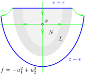
Figure 1: $(N,L)$ for isolated $x\in{\rm Crit}f$

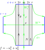
Figure 2: Non-degenerate $x$

$$L=L_{x}^{{\varepsilon},\tau}:=\{p\in N\mid f(\varphi_{2\tau}p)\leq c-{\varepsilon}\}.$$ (1.2)

By Sard’s theorem we may suppose that $c\pm{\varepsilon}$ are regular values of $f$; otherwise, perturb ${\varepsilon}$. Note that in case of a local minimum $x$ the set $N$ is a local sublevel set and $L$ is empty (any point near $x$ eventually gets stuck on the level $c$ of $x$, so none reaches the lower level $c-{\varepsilon}$).
In fact, for small ${\varepsilon}$ and large $\tau$ it holds that (i) the fixed point $x$ of $\varphi$ lies in the interior of $N$ but not in $L$, (ii) there are no other fixed points in $N$, (iii) the subset $L$ is positively invariant in $N$, and (iv) $L$ is an exit set of $N$ in the sense that every forward flow line which leaves $N$ runs through $L$ first; for details see Definition 2.1. For a proof of (i–iv) in the non-degenerate case see [19]; see [21] for an infinite dimensional context.

In the more general isolated case, meaning that $x$ is just required to be an isolated critical point of $f$, properties (i–iv) will be established in Theorem 2.3 below. Such $(N,L)$ is called a Conley pair, and $N$ a Conley block, for the isolated critical point $x$. Note that the part of the stable manifold $W^{s}=W^{s}(x)$ in $N$ is the ascending disk $W^{s}_{\varepsilon}=W^{s}_{\varepsilon}(x):=W^{s}(x)\cap\{f\leq f(x)+{\varepsilon}\}$.
By the Shrinking Lemma 2.2 one can fit $N$ into any given neighborhood of an isolated $x\in{\rm Crit}f$ by picking ${\varepsilon},\tau>0$ sufficiently small and large, respectively.

Dynamical thickening – non-degenerate case

For non-degenerate critical points $x$ much more can be shown for small ${\varepsilon}$ and large $\tau$: Firstly, the set $N=N_{x}^{{\varepsilon},\tau}$ contracts onto the ascending disk $W^{s}_{\varepsilon}$, as $\tau\to\infty$.

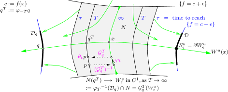
Figure 3: Dynamical thickening $(N,\theta)$ of $(W^{s}_{\varepsilon},\varphi_{\geq 0})$

Secondly, the set $N$ is fibered by diffeomorphic copies of $W^{s}_{\varepsilon}$, one copy for each point of the part $W^{u}_{{\varepsilon},\tau}:=N\cap W^{u}$ of the unstable manifold $W^{u}=W^{u}(x)$ in $N$; see Figure 3. The construction of the fiber bundle $W^{s}_{\varepsilon}\hookrightarrow N\to W^{u}_{{\varepsilon},\tau}$ starts with a choice of fibers in the lower level set: Endow some neighborhood ${\mathcal{D}}$ of the descending sphere $S^{u}_{\varepsilon}=S^{u}_{\varepsilon}(x):=W^{u}(x)\cap\{f=c-{\varepsilon}\}$ in the level set $\{f=c-{\varepsilon}\}$ with the structure of a disk bundle ${\mathbb{D}}\hookrightarrow{\mathcal{D}}\to S^{u}_{\varepsilon}$ where the codimension of the disk ${\mathbb{D}}$ is given by the Morse index $k={\rm ind}_{f}(x)$. For $q\in S^{u}_{\varepsilon}$ and $T\geq\tau$ the fiber $N(q^{T})$ over $q^{T}:=\varphi_{-T}q$ by definition is the part in $N$ of the pre-image ${\varphi_{T}}^{-1}{\mathcal{D}}_{q}$ of the fiber ${\mathcal{D}}_{q}$. Let the fiber over $x$ be those points that never reach ${\mathcal{D}}$, namely $N(x):=W^{s}_{\varepsilon}$. One shows [19, 21] that each fiber $N(q^{T})$ can be written as a $C^{1}$ graph over $W^{s}_{\varepsilon}$ or, in other words, as the image of a $C^{1}$ embedding ${\mathcal{G}}^{T}_{q}:W^{s}_{\varepsilon}\to M$. Transfer the forward semi-flow $\varphi_{\geq 0}$ on $W^{s}_{\varepsilon}$ to each fiber via conjugation by the graph maps; see Figure 3.

• Dynamical thickening $(N,\theta)$ of $(W^{s}_{\varepsilon},\varphi_{\geq 0})$. As just described $N$ carries the structure of a fiber bundle $W^{s}_{\varepsilon}\hookrightarrow N\to W^{u}_{{\varepsilon},\tau}$ equipped with a fiberwise forward semi-flow $\theta$. Fibers and flow are modeled on the ascending disk $W^{s}_{\varepsilon}$ equipped with $\varphi_{\geq 0}$ and defined as graphs over $W^{s}_{\varepsilon}$ and by conjugation. Hence $\theta$ deforms the total space $N$ into the base space $W^{u}_{{\varepsilon},\tau}:=N\cap W^{u}$; see Figures 2 and 3.

• Morse filtration. Dynamical thickening was introduced in [21] to construct a Morse filtration of a loop space in order to represent Morse homology for semi-flows in terms of singular homology. For an overview see [18].

• Flow selector. Dynamical thickening was applied in [20] to prove the cell attachment theorem in Morse theory [13, Thm. 3.1] through a basic two step deformation. Here entered crucially the construction of a flow selector ${\mathcal{S}}^{+}$, namely a hypersurface transverse to two flows, which came up in [12] in two flavors, via Conley pairs and via a carving technique. The point is that transversality allows to switch along ${\mathcal{S}}^{+}$ from one to the other flow in a continuous fashion.

• CW decomposition. It is an old believe that the closures of the unstable manifolds of a Morse-Smale gradient flow $\varphi$ of a Morse function $f$ on a closed manifold $M$ provide a CW decomposition of $M$. If the Riemannian metric is Euclidean near the critical points this is a result of Kalmbach [8]; see also Laudenbach in [2]. In the general cases two methods of proof have been proposed in [16] and [9].

  Here is a geometric approach via asymptotic extensions of dynamical thickenings arising from joint ideas in [11, 12]. But so far this only works in dimension two (where the problem of compatibly organizing fibers on overlaps is void). Whereas the flow $\varphi$ serves to identify diffeomorphically an unstable manifold with an open unit disk, this identification does not extend continuously to the boundary: In Figure 4 the endpoints of the $\color[rgb]{0,1,0}\varphi$ flow lines do not even fill the boundary $\Delta$ of the unstable manifold $W$.

  

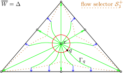
  Figure 4: Curves $\Gamma_{q}$ composed of flows $\varphi$ and $\theta^{1}$ partition $W=W^{u}(x)$

  Now extend each dynamical thickening $(N_{1},\theta^{1})$ of an index 1 point down to level $c_{1}-{\varepsilon}_{1}$ via $\varphi$ and then move the fibers that lie on level $c_{1}-{\varepsilon}_{1}$ further down all the way via the level preserving diffeomorphisms $\hat{\varphi}_{t}$ generated by the vector field $X=-\nabla f/\mathopen{\|}\nabla f\mathclose{\|}^{2}$ on $M\setminus{\rm Crit}f$. We get a fiber bundle ${\mathcal{U}}_{1}\to W$ that contains $N_{1}$ and carries a fiberwise forward flow defined via conjugation by the $\hat{\varphi}_{t}$ and still denoted by $\theta^{1}$.
  To make the dynamical thickening $({\mathcal{U}}_{1},\theta^{1})$ forward $\varphi$-attractive one constructs a flow selector ${\mathcal{S}}_{1}^{+}\subset{\mathcal{U}}_{1}$ and throws away from each fiber of ${\mathcal{U}}_{1}$ the part outside ${\mathcal{S}}_{1}^{+}$: Distribute the entrance hypersurface $N_{1}^{+}$, see (2.9) and Figure 6, utilizing a monotone smooth function, similar in spirit to [20], to obtain a flow selector ${\mathcal{S}}_{1}^{+}:=\Phi N_{1}^{+}\subset{\mathcal{U}}_{1}$ that bounds a $\varphi$-attractive fiber bundle ${\mathcal{S}}_{1}:=\Phi N_{1}\to W$. (A fiber of ${\mathcal{S}}_{1}\subset{\mathcal{U}}_{1}$ arises from a fiber of ${\mathcal{U}}_{1}$ by throwing away the part not enclosed by ${\mathcal{S}}_{1}^{+}$. The fibers of ${\mathcal{S}}_{1}$ are invariant under $\theta^{1}$.) This defines the $\varphi$-attractive dynamical thickening $({\mathcal{S}}_{1}:=\Phi N_{1},{\color[rgb]{0,0,1}\theta^{1}})$. The dotted line in Figure 4 shows the flow selector ${\mathcal{S}}_{1}^{+}$. The curves $\Gamma_{q}$ are composed of $\color[rgb]{0,1,0}\varphi$ trajectories followed by $\color[rgb]{0,0,1}\theta^{1}$ trajectories – transition taking place along the flow selector ${\mathcal{S}}_{1}^{+}$. The curves $\Gamma_{q}$ partition the unstable manifold $W$ of $x$ and its endpoints cover the boundary $\Delta$. The endpoints of the $\Gamma_{q}$ vary continuously in the elements $q$ of the descending sphere $\color[rgb]{1,0,0}S^{u}_{\varepsilon}$ as both $\color[rgb]{0,1,0}\varphi$ and $\color[rgb]{0,0,1}\theta^{1}$ are transverse to the hypersurface ${\mathcal{S}}_{1}^{+}$.

Organization of this paper. In Section 2 we prove the defining properties (i–iv) for Conley pairs $(N,L)$ associated to isolated critical points and construct the open contractible thickenings of the stable manifolds yet missing in the proof of the Lusternik-Schnirelmann Theorem 1.1. Section 3 reviews further tools to detect critical points: Cuplength in cohomology, its dual cousin the subordination number, and a variant $\mathrm{cat^{a}}(M)$ of the LS category called ambient LS category. For further reading, concerning LS theory, we recommend the comprehensive monograph [5] or the more elementary concise presentation in [22, IV.3].

Acknowledgements. The author would like to thank brazilian tax payers for excellent teaching and research conditions at UNICAMP.

For convenience of the reader we conclude the introduction by introducing these tools and summarize their interactions. Throughout $R$ is a commutative ring:

Cuplength

The $R$-cuplength $\mathrm{cup}_{R}(X)$ of a topological space $X$ is the largest integer $k\in{\mathbb{N}}$ such that there exist $k$ cohomology classes $\text{\boldmath$\alpha_{1}$},\dots,\text{\boldmath$\alpha_{k}$}$ of positive degree (grading) in the cohomology ring ${\rm H}^{*}={\rm H}^{*}(X;R)$ whose cup product is non-zero

$$\text{\boldmath$\alpha_{1}$}\mathop{\cup}\dots\mathop{\cup}\text{\boldmath$\alpha_{k}$}\not=0.$$ (1.3)

If no such classes exist (cohomology in positive degree is $0$), set $\mathrm{cup}_{R}(X)=0$. Recall that degrees add up under $\cup:{\rm H}^{k}\times{\rm H}^{\ell}\to{\rm H}^{k+\ell}$ and ${\rm H}^{k>\dim M}(M)=0$ for manifolds. So the positive degree assumption implies the finiteness estimate

$$\mathrm{cup}_{R}(M)\leq\dim M$$ (1.4)

for any connected manifold $M$. Many $R$-cuplengths of many common manifolds are known; see e.g. [5, §1.2]. This, together with the key estimate $\mathopen{|}{\rm Crit}f\mathclose{|}>\mathrm{cup}_{R}(M)$, see (1.5) below, makes $\mathrm{cup}_{R}$ a rather useful quantity.

Subordination

For non-trivial homology classes $\text{\boldmath$b_{1}$},\text{\boldmath$b_{2}$}\in{\rm H}_{*}(M;R)\setminus\{0\}$ of a closed manifold $M$ one writes $\text{\boldmath$b_{1}$}<\text{\boldmath$b_{2}$}$ and says $b_{1}$ is subordinated to $b_{2}$, if there is a cohomology class $\text{\boldmath$\omega$}\in{\rm H}^{p>0}$ of positive degree such that

$$\text{\boldmath$b_{1}$}=\text{\boldmath$\omega$}\mathop{\cap}\text{\boldmath$b_{2}$}$$

where $\mathop{\cap}:{\rm H}^{p}\times{\rm H}_{m}\to{\rm H}_{m-p}$ is the cap product. Subordination is transitive and the degree strictly increases. The $R$-subordination number $\mathrm{sub}_{R}(M)$ is the largest integer $k\in{\mathbb{N}}$ such that there is a chain of $k$ subordinated classes

$$\text{\boldmath$b_{1}$}<\text{\boldmath$b_{2}$}<\dots<\text{\boldmath$b_{k}$}<\text{\boldmath$b_{k+1}$}.$$

The significance of subordination lies in the fact that existence of classes $\text{\boldmath$b_{1}$}<\text{\boldmath$b_{2}$}$ guarantees existence of two different critical values, thus critical points, for any $C^{2}$ function $f$ whose critical points are all isolated; see Theorem 3.13 (Lusternik-Schnirelmann refined minimax principle).

Inequalities and comparisons

For a closed manifold $M$ equipped with a $C^{2}$ function $f$ there are the inequalities

$$\left|{\rm Crit}f\right|\geq\mathrm{cat^{a}}(M)\geq\mathrm{cat}(M)>\mathrm{cup}_{R}(M)=\mathrm{sub}_{R}(M)$$ (1.5)

where $R$ is any commutative ring. In the non-degenerate (Morse) case it holds

$$\left|{\rm Crit}f\right|\geq\dim{\rm H}_{*}(M;{\mathbb{F}})\geq 1+\mathrm{sub}_{\mathbb{F}}(M).$$ (1.6)

for any field ${\mathbb{F}}$. All these inequalities will be proved below.

For any given field ${\mathbb{F}}$ Morse theory gives by (1.6) stronger (or equal) critical point estimates than subordination/cuplength. In contrast, category can be superior to Morse theory, depending on the field. Indeed

$$\dim{\rm H}_{*}({\mathbb{R}}{\rm P}^{2};{\mathbb{Q}})=1+0+0<3=\mathrm{cat}({\mathbb{R}}{\rm P}^{2}).$$ (1.7)

But in case of ${\mathbb{R}}{\rm P}^{2}$ there still exists a field bringing back Morse theory, namely

$$\dim{\rm H}_{*}({\mathbb{R}}{\rm P}^{2};{\mathbb{Z}}_{2})=1+1+1=\mathrm{cat}({\mathbb{R}}{\rm P}^{2}).$$

Is this a general fact? For simply connected orientable manifolds the answer is yes: These satisfy $\dim{\rm H}_{*}(M;{\mathbb{Q}})\geq\mathrm{cat}(M)$ by [5, Ex. 1.33, cf. p. 291].

2 Conley pairs for isolated critical points

Definition 2.1.

Let $\phi=\{\phi_{t}\}$ be a continuous flow on a topological space $X$. A Conley pair $(N,L)$ for an isolated fixed point $x$ of $\phi$ consists of a pair of compact subspaces $(N,L)$ of $X$ which satisfy

1. $x\in\accentset{\circ}{N}\setminus L$

2. $N\cap{\rm Fix}\,\phi=\{x\}$

3. $p\in L$ and $\phi_{[0,t]}p\subset N\,\Rightarrow\,\phi_{t}p\in L$

4. $p\in N$ and $\phi_{T}p\notin N\;\Rightarrow\;\exists\sigma\in[0,T):\phi_{\sigma}p\in L$ and $\phi_{[0,\sigma]}p\subset N$

In particular, conditions (i) and (ii) tell that $N$ is a neighborhood of $x$ which contains no other critical points in its closure. Condition (iii) says that $L$ is positively invariant in $N$ and (iv) asserts that every semi-flow line which leaves $N$ goes through $L$ before exiting. Hence we say that $L$ is an exit set of $N$; cf. Figures 2 and 2. The set $N$ is also called a Conley block. Note that in this generality, as opposed to the realization (1.1) of $(N,L)$ for downward gradient flows, there is no obstruction that exiting points would re-enter $N$. For downward gradient flows the assumption in (iii) is equivalent to (2.8).

Coming back to gradient flows suppose from now on, throughout Section 2, that $f:M\to{\mathbb{R}}$ is a $C^{2}$ function on a closed Riemannian manifold $(M,g)$.

Preparing the next two proofs. Pick two regular values $a<b$ of $f$ such that there is only one critical value $c$ in between them which, moreover, is their mean $c=\frac{a+b}{2}$. By $f:f^{-1}[a,b]\to[a,b]$ we denote the restriction to the (compact) domain $f^{-1}[a,b]$. Let $\varphi$ be the corresponding (local downward) gradient flow. Furthermore, suppose that $x$ is an isolated critical point of $f$. Let $(N,L)$ be defined by (1.1) and (1.2) with constants ${\varepsilon}\in(0,\frac{b-a}{2}]$ and $\tau\geq 1$.

Lemma 2.2 (Shrink to critical point).

Let $U_{x}$ be a neighborhood in $f^{-1}[a,b]$ of the isolated critical point $x$ of $f$. Then there are constants ${\varepsilon}_{*}>0$ and $\tau_{*}\geq 1$ such that $N_{x}^{{\varepsilon}_{*},\tau_{*}}$ is contained in $U_{x}$.

Proof.

Write the set of critical points of $f:f^{-1}[a,b]\to[a,b]$ as disjoint union $\{x\}\mathop{\dot{\cup}}C$ of two (compact) subsets. Pick disjoint open neighborhoods $U$ of $x$ and $V$ of $C$. Suppose that $U\subset U_{x}$; otherwise, replace $U$ by $U\cap U_{x}$. Observe that the complement $K$ of $U\cup V$ is compact and contains no critical points.

Now suppose by contradiction that the set $N_{x}^{{\varepsilon},\tau}$ was not contained in $U$ for all ${\varepsilon},\tau$. Then there are sequences ${\varepsilon}_{\nu}\searrow 0$ and $\tau_{\nu}\nearrow\infty$ such that $N_{\nu}:=N_{x}^{{\varepsilon}_{\nu},\tau_{\nu}}\not\subseteq U$, that is $N_{\nu}\setminus U\not=\emptyset$, for every $\nu\in{\mathbb{N}}$. More is true, namely

$$N_{\nu}\setminus(U\cup V)\not=\emptyset.$$

Thus there is a sequence $p_{\nu}\in N_{\nu}\setminus(U\cup V)\subset K$ and a subsequence, still denoted by $p_{\nu}$, that converges to some point $p\in K$, as $\nu\to\infty$; see Figure 5.

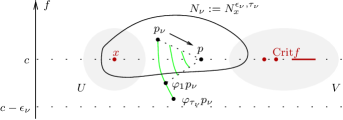
Figure 5: Proof of the shrinking Lemma 2.2

The fact that $p_{\nu}\in N_{\nu}$ implies firstly that $f(p)\leq c$, since $f(p_{\nu})\leq c+{\varepsilon}_{\nu}$, and secondly that $f(\varphi_{1}p)\geq c$, since $f(\varphi_{1}p_{\nu})\geq f(\varphi_{\tau_{\nu}}p_{\nu})\geq c-{\varepsilon}_{\nu}$. Since a downward gradient flow strictly decreases $f$, except at critical points, we get for $t\in[0,1]$ that

$$c\geq f(p)\geq f(\varphi_{t}p)\geq f(\varphi_{1}p)\geq c,$$

i.e. $f(\varphi_{t}p)\equiv c$, $\forall t\in[0,1]$. So $p\in K$ is a critical point of $f$. Contradiction. ∎

Theorem 2.3 (Conley pair).

The pair $(N,L)$ defined by (1.1–1.2) is a Conley pair for an isolated fixed point $x$ of $\varphi$ for all ${\varepsilon}>0$ small and $\tau\geq 1$ large.

Remark 2.4 (No re-entry).

Since we work with a downward gradient flow $\varphi$ the function $f$ decays along trajectories. Now observe that a point which leaves $N$ will precisely $\tau$ time units later run through the level $c-{\varepsilon}$. But $N$ itself sits strictly above that level. Therefore a point which exits $N$ cannot re-enter.

Proof of Theorem 2.3.

We need to verify properties (i–iv) in Definition 2.1.

(i) Because $f(x)=c$ and the critical point $x$ is a fixed point of $\varphi$ it is clear that $x\in N$ by definition (1.1). Since $f$ and $f\circ\varphi_{\tau}$ are continuous $x$ lies in the interior of $N$. One has $x\notin L$, because $f(\varphi_{2\tau}x)=f(x)=c$.

(ii) True by the shrinking Lemma 2.2. Here isolatedness of $x$ enters.

(iii) As $f$ decreases along $\varphi$, the assumption in (iii) is equivalent to

$$p\in L\quad\wedge\quad\varphi_{t}p\in N,$$ (2.8)

for some $t\geq 0$. This implies that $\varphi_{t}p\in L$: Indeed $\varphi_{t}p\in N$ by assumption and

$$f(\varphi_{2\tau}\varphi_{t}p)\leq f(\varphi_{2\tau}p)\leq c-{\varepsilon}.$$

Step one uses $t\geq 0$ and that $f$ decreases along $\varphi$. Step two holds since $p\in L$.

(iv) Suppose $p\in N$ and $\varphi_{T}p\notin N$ for some $T>0$. There are two cases. Case 1: $p\in L$. Pick $\sigma=0$.

Case 2: $p\in N\setminus L$. Note that $N\setminus L$ is open in $N$. We need to find a time $\sigma\in(0,T)$ such that $\varphi_{\sigma}p\in L$ and $\varphi_{[0,\sigma]}p\subset N$. By (ii) the only critical point in $N$ is $x$. The assumptions imply firstly that $p$ is not a critical point, but is connected to $x$ inside $N$ through a continuous path, and secondly that

$$f(p)\leq c+{\varepsilon},\qquad f(\varphi_{2\tau}p)>c-{\varepsilon},\qquad f(\varphi_{\tau+T}p)<c-{\varepsilon}.$$

We will show that these three inequalities imply that, firstly, there is a unique time $\alpha>0$ until which the trajectory through $p\in N\setminus L$ remains in $N$ and at which it enters $L$ and, secondly, that there is a unique time $\beta\in(\alpha,T)$ at which the trajectory leaves $L$, hence by (iii) simultaneously $N$, forever (Remark 2.4). Given $\alpha$ and $\beta$, any $\sigma\in[\alpha,\beta]\subset(0,T)$ satisfies the conclusion of (iv).

To define the entrance time $\alpha>0$ observe that by inequalities two and three, together with the fact that $f$ decays along $\varphi$, the trajectory through $p\in N\setminus L$ runs through the level set $\{f=c-{\varepsilon}\}$ at a unique time $\text{\boldmath$T_{*}$}\in(2\tau,\tau+T)$. Set

$$\alpha:=T_{*}-2\tau>0$$

to obtain $c-{\varepsilon}=f(\varphi_{T_{*}}p)=f(\varphi_{2\tau+\alpha}p)$. To get $T_{*}=2\tau+\alpha=\tau+\beta$ define

$$\beta:=\alpha+\tau\geq\alpha+1.$$

So the identity reads $c-{\varepsilon}=f(\varphi_{\tau+\beta}p)$. Thus $\beta<T$ by inequality three.

It remains to show, firstly, that $\alpha>0$ is the unique time at which the trajectory through $p\in N\setminus L$ enters $L$ and at least until which it lies in $N$ and, secondly, that $\beta$ is the unique time when the trajectory leaves $L$, thus $N$. More precisely, we show, firstly, that $\varphi_{s}p\in N$ for some $s\geq 0$ if and only if $s\in[0,\beta]$ and, secondly, that $\varphi_{s}p\in L$ for some $s>0$ if and only if $s\in[\alpha,\beta]$.
Assertion 1. Pick $s\in[0,\beta]$. Then $f(\varphi_{s}p)\leq f(p)\leq c+{\varepsilon}$ since $p\in N$. Furthermore, note that $\tau+s\leq\tau+\beta=T_{*}$. So $f(\varphi_{\tau}(\varphi_{s}p))\geq f(\varphi_{T_{*}}p)=c-{\varepsilon}.$ Moreover, via $[0,s]\ni t\mapsto\varphi_{t}p$, the point $\varphi_{s}p$ path-connects inside $N$ to $p$ which in turn path-connects inside $N$ to $x$ by definition of $p\in N$. This proves that $\varphi_{s}p\in N$. Vice versa, assume $\varphi_{s}p\in N$ for some $s\geq 0$. The desired inequality $s\leq\beta$ is equivalent to $s+\tau\leq T_{*}$. As $f(\varphi_{T_{*}}p)=c-{\varepsilon}$, the latter inequality follows from the consequence $f(\varphi_{\tau+s}p)\geq c-{\varepsilon}$ of the assumption $\varphi_{s}p\in N$ and the gradient flow property that $f$ decreases along the trajectory.
Assertion 2. Pick $s\in[\alpha,\beta]$. Then $\varphi_{s}p\in N$ by assertion 1. It remains to show $f(\varphi_{2\tau}(\varphi_{s}p))\leq c-{\varepsilon}$. This holds true since $c-{\varepsilon}=f(\varphi_{T_{*}}p)$ and $2\tau+s\geq 2\tau+\alpha=T_{*}$ by choice of $s$ and definition of $\alpha$. Vice versa, assume $\varphi_{s}p\in L$ for some $s>0$. Then we get the two inequalities $f(\varphi_{\tau}(\varphi_{s}p))\geq c-{\varepsilon}$ and $f(\varphi_{2\tau}(\varphi_{s}p))\leq c-{\varepsilon}$ by definition of $L$. If $s>\beta$, equivalently $s+\tau>\beta+\tau=T_{*}$, we get $f(\varphi_{s+\tau}p)<f(\varphi_{T_{*}}p)=c-{\varepsilon}$ contradicting inequality one. In the case $s\in(0,\alpha)$ we get $f(\varphi_{2\tau+s}p)>f(\varphi_{T_{*}}p)=c-{\varepsilon}$ contradicting inequality two. ∎

Thickenings of (un)stable manifolds via Conley pairs

Proposition 2.5.

Suppose $f$ is a $C^{2}$ function on a closed Riemannian manifold $(M,g)$ with isolated, thus finitely many, critical points, say $x_{1},\dots,x_{\ell}$. Then

• there is an open cover $\{{\mathcal{W}}_{i}\}_{i=1}^{\ell}$ of $M$ by nullhomotopic thickenings of the unstable manifolds, that is each ${\mathcal{W}}_{i}$ is open in $M$, contains the unstable manifold $W_{i}$ of $x_{i}$, and is nullhomotopic to $x_{i}$;

• there is an open cover $\{{\mathcal{U}}_{i}\}_{i=1}^{\ell}$ of $M$ where each ${\mathcal{U}}_{i}$ is ambient  nullhomotopic to $x_{i}$ (and covers ’large parts’ of the unstable manifold).

Thickenings corresponding to critical points on the same level set are pairwise disjoint. Furthermore, there are analogous open covers $\{{\mathcal{W}}_{i}^{*}\}_{i=1}^{\ell}$ and $\{{\mathcal{U}}_{i}^{*}\}_{i=1}^{\ell}$ corresponding to the stable manifolds.

Proof.

The proof takes three steps (0), (i), (ii). Step (0) is taken from [7].

(0) Each critical point $x_{i}$ has an ambient nullhomotopic open neighborhood $V_{i}$: As the critical points $x_{i}$ are isolated, there are pairwise disjoint local coordinate charts $\{(\psi_{i},U_{i})\}_{i=1}^{\ell}$ such that $U_{i}$ contains no critical point except $x_{i}$. Pick an open ball about $\tilde{x}_{i}:=\psi_{i}(x_{i})$ contained in $\tilde{U}_{i}:=\psi_{i}(U_{i})$ and another open ball $\tilde{V}_{i}$ about $\tilde{x}_{i}$ of, say, half the radius of ball one. There is a simple radial homotopy of smooth maps that deforms the closure of the smaller ball to its center $\tilde{x}_{i}$ while the points in the complement of the larger ball remain fixed; just stretch the annulus. Set $V_{i}:={\psi_{i}}^{-1}\tilde{V}_{i}$. Note that by construction the closures ${\macc@depth\char 1\relax\frozen@everymath{\macc@group}\macc@set@skewchar\macc@nested@a 111{V}}_{{\mspace{-5.0mu}i}}$ are pairwise disjoint and also ambient nullhomotopic.

(i) A way to control the problem of multiple entrance and exit times is to use a Conley pair $(N_{i},L_{i})$ for $x_{i}$ as provided by Theorem 2.3.

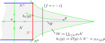
Figure 6: Thickening ${\mathcal{W}}$ of $W=W^{u}(x)$ as Conley block forward exhaustion

By isolatedness of $x_{i}$ the shrinking Lemma 2.2 applies and we may suppose that $N_{i}\subset V_{i}$. Since the $V_{i}$ are pairwise disjoint, so are the $N_{i}$. Actually we need here only the ’outmost’ points of the exit set $L_{i}$, namely, the so-called exit locus

$${\color[rgb]{1,0,0}N_{i}^{-}}:=\left(\{f<c_{i}+{\varepsilon}_{i}\}\cap{\varphi_{\tau_{i}}}^{-1}\{f=c_{i}-{\varepsilon}_{i}\}\right)_{N_{i}},\quad c_{i}:=f(x_{i}),$$

that consists of those points of $N_{i}=N^{{\varepsilon}_{i},\tau_{i}}_{x_{i}}$ which lie below the upper level set and reach the lower one precisely in time $\tau_{i}$. Here $(\dots)_{N_{i}}$ selects those connected components that lie in $N_{i}$. Similarly there is the entrance locus

$${\color[rgb]{0,0,1}N_{i}^{+}}:=\left\{p\in\{f=c_{i}+{\varepsilon}_{i}\}\mid f(\varphi_{\tau_{i}}p)>c_{i}-{\varepsilon}_{i}\right\}_{N_{i}}$$ (2.9)

and the bounce off locus

$$\begin{split}N_{i}^{0}&:=\left\{p\in N_{i}\cap\{f=c_{i}+{\varepsilon}_{i}\}\mid f(\varphi_{\tau_{i}}p)=c_{i}-{\varepsilon}_{i}\right\}\\ &\,\,=\left(\{f=c_{i}+{\varepsilon}_{i}\}\pitchfork{\varphi_{\tau_{i}}}^{-1}\{f=c_{i}-{\varepsilon}_{i}\}\right)_{N_{i}}.\end{split}$$

Note that $N_{i}^{-}$ and $N_{i}^{+}$ are open subsets of the hypersurfaces ${\varphi_{\tau_{i}}}^{-1}\{f=c_{i}-{\varepsilon}_{i}\}$ and $\{f=c_{i}+{\varepsilon}_{i}\}$, respectively, whereas $N_{i}^{0}$ consists of components of their transverse intersection. So the $N_{i}^{\pm}$ are non-compact hypersurfaces of $M$ and $N_{i}^{0}$ is a closed codimension 2 submanifold. Let ${\mathcal{N}}_{i}$ be the interior and $\dot{N}_{i}$ the topological boundary of the Conley block $N_{i}$. Figure 6 illustrates the partitions

$$\dot{N}_{i}={\color[rgb]{0,0,1}N_{i}^{+}}\mathop{\dot{\mathop{\cup}}}N_{i}^{0}\mathop{\dot{\mathop{\cup}}}{\color[rgb]{1,0,0}N_{i}^{-}},\qquad N_{i}={\mathcal{N}}_{i}\mathop{\dot{\mathop{\cup}}}\dot{N}_{i},\qquad{\mathcal{N}}_{i}:=\accentset{\circ}{N}_{i}.$$ (2.10)

Define the desired thickening to be the forward exhaustion of the interior ${\mathcal{N}}_{i}$ of the Conley block $N_{i}$, namely

$${\mathcal{W}}_{i}:=\varphi_{[0,\infty)}{\mathcal{N}}_{i}:=\bigcup_{t\geq 0}\varphi_{t}{\mathcal{N}}_{i}.$$

The set ${\mathcal{W}}_{i}$ is open in $M$ and contains the whole unstable manifold $W_{i}$ along which it extends. A homotopy $h_{\lambda}:{\mathcal{W}}_{i}\to M$, $\lambda\in[0,1]$, between the inclusion $h_{0}:{\mathcal{W}}_{i}\hookrightarrow M$ and a map $h_{1}:{\mathcal{W}}_{i}\to M$ whose image lies in $N_{i}$ is given by

$$\begin{split}h:{\rm I}\times{\mathcal{W}}_{i}\to M,\quad(\lambda,p)\mapsto\begin{cases}p&\text{, $p\in{\mathcal{W}}_{i}\cap N_{i}$,}\\ \varphi_{\lambda{\mathcal{T}}(p)}p&\text{, $p\in{\mathcal{W}}_{i}\setminus N_{i}$.}\end{cases}\end{split}$$

Here ${\mathcal{T}}(p)<0$ is the arrival time of $p\in{\mathcal{W}}_{i}\setminus N_{i}$ at the exit locus $N_{i}^{-}$. It is well defined since such $p$ comes from the interior of $N_{i}$ by definition of ${\mathcal{W}}_{i}$, so it must have left through the exit set $L_{i}$, thus through $N_{i}^{-}$, by property (iv) in Definition 2.1. This is illustrated by Figure 6 in terms of the orbit ${\mathcal{O}}(p)$ through $p$. That orbit is orthogonal to the lower level set $\{f=c_{i}-{\varepsilon}_{i}\}$, hence still transverse to the time $-\tau_{i}$ copy $N_{i}^{-}$. But this means that the arrival time ${\mathcal{T}}(p)$ varies continuously in $p$. The piecewise definition of $h$ also matches continuously: For a point $p\in{\mathcal{W}}_{i}\setminus N_{i}$ close to the other set ${\mathcal{W}}_{i}\cap N_{i}={\mathcal{N}}_{i}\cup N_{i}^{-}$, hence close to $N_{i}^{-}$, the arrival time approaches 0, so $\varphi_{{\mathcal{T}}(p)}p$ approaches $p$.

The desired contraction is then given by the homotopy $h$ from ${\mathcal{W}}_{i}$ to $N_{i}\subset V_{i}$ followed by the ambient nullhomotopy in Step (0) of $V_{i}$ onto the critical point $x_{i}$. The collection ${\mathcal{W}}_{1},\dots,{\mathcal{W}}_{\ell}$ covers $M$ since already the unstable manifolds do. Those ${\mathcal{W}}_{i}$ corresponding to critical points on the same level, say $c$, are pairwise disjoint: Indeed the $V_{i}$, thus the ${\mathcal{N}}_{i}$, are and every point $p$ of ${\mathcal{W}}_{i}$ outside ${\mathcal{N}}_{i}$ has left through the exit locus $N_{i}^{-}\subset L_{i}$. Thus $p$ has crossed or will cross level $c-{\varepsilon}_{i}$ by definition of $L_{i}$. But such flow line cannot enter any of the other ${\mathcal{W}}_{j}$’s since their entrance loci $N_{j}^{+}$ lie on the higher level $c+{\varepsilon}_{j}$.

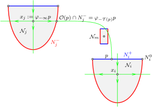
Figure 7: Backward entrance time ${\mathcal{T}}_{i}^{+}:N_{i}^{+}\to{\mathbb{R}}_{+}$ and $N_{i}$ for $f=-u_{1}^{2}+u_{2}^{3}$

(ii) After handy first tries we start from scratch and, for a change, emphasize stable manifolds and backward flow in order to construct ambient contractible sets ${\mathcal{U}}_{i}^{*}$ that crawl up the stable manifolds and are of the form $\varphi_{-T_{i}}{\mathcal{N}}_{i}$. (Replace $f$ by $-f$ to get ${\mathcal{U}}_{i}$.) For each of the $\ell$ critical points $x_{i}$ of $f$ pick a Conley pair $(N_{i},L_{i})$ as in Theorem 2.3. By finiteness of ${\rm Crit}f$ suppose that all of these pairs are defined with respect to the same constants ${\varepsilon}$ and $\tau$ chosen, in addition, such that $N_{i}\subset V_{i}$ by the Shrinking Lemma 2.2. By Step (0) the $N_{i}$ are pairwise disjoint. As earlier ${\mathcal{N}}_{i}$ denotes the interior of $N_{i}$.
For each critical point $x_{i}$ set $c_{i}:=f(x_{i})$ and consider the function

$${\mathcal{T}}_{i}^{+}:N_{i}^{+}\to(0,\infty),$$

as illustrated by Figure 7, that maps a point $p$ of the entrance locus ${\color[rgb]{0,0,1}N_{i}^{+}}\subset\{f=c_{i}+{\varepsilon}\}$ to the time ${\mathcal{T}}_{i}^{+}(p)$ at which the backward flow of $p$ meets the exit locus ${\color[rgb]{1,0,0}N_{j}^{-}}$ associated to $p$’s asymptotic origin $x_{j}:=\varphi_{-\infty}p$.

Remark. Note that $\varphi_{-{\mathcal{T}}_{i}^{+}(p)}p$ lies in the boundary of the descending disk $W^{u}_{\varepsilon}(x_{j})$, hence $\varphi_{-\mu-{\mathcal{T}}_{i}^{+}(p)}p$ lies in its interior, hence in ${\mathcal{N}}_{j}$, whenever $\mu>0$.

The number ${\mathcal{T}}_{i}^{+}(p)$ is well defined and finite, because the asymptotic backward limit $\varphi_{-\infty}p:=\lim_{t\to-\infty}\varphi_{t}p$ exists and is a critical point, say $x_{j}$, which sits inside the Conley block $N_{j}$. Since any two Conley blocks are disjoint the time ${\mathcal{T}}_{i}^{+}(p)>0$ is positive. Although the function ${\mathcal{T}}_{i}$ might be highly discontinuous (perturb $p$ in Figure 7 slightly to the right), it is bounded: The closures of $N_{i}^{+}$ and the finitely many higher lying $N_{j}^{-}$ are all compact and, most importantly, they contain no critical points by Theorem 2.3. For each critical point $x_{i}$ set

$${\mathcal{T}}_{i}:=1+\sup_{N_{i}^{+}}{\mathcal{T}}_{i}^{+}\in[0,\infty)$$

where the convention $\sup_{\emptyset}{\mathcal{T}}_{i}^{+}:=0$ takes care of local maxima.

Not a good idea. One might try for the required open ambient nullhomotopic cover of $M$ the sets ${\mathcal{U}}_{i}^{*\prime}:={\varphi_{{\mathcal{T}}_{i}}}^{-1}{\mathcal{N}}_{i}$ (or utilize some uniform time, say ${\mathcal{T}}_{*}:=\max_{i}{\mathcal{T}}_{i}$, and try ${\mathcal{U}}_{i}^{*\prime\prime}:={\varphi_{T_{*}}}^{-1}{\mathcal{N}}_{i}$). The proof below will work – except for the final argument, case 2 b). The problem will be that with this choice one does get back from $N_{i}^{+}$ to $N_{j}^{-}$, but the relevant set to backward-enter ${\mathcal{U}}_{j}$ is ${\varphi_{T_{j}}}^{-1}N_{j}^{-}$ which sits way further in the past. This indicates that one should define the sets ${\mathcal{U}}_{i}$ successively according to the level of $x_{i}$ starting with the highest one and adding ’extra backward time’ in the definition of the lower level ${\mathcal{U}}_{i}$’s.

Definition of ${\mathcal{U}}_{1}^{*},\dots,{\mathcal{U}}_{\ell}^{*}$. Suppose there are $\ell$ critical points of $f$ and these are enumerated such that $c_{1}=f(x_{1})\leq\dots\leq c_{\ell}=f(x_{\ell})$. Set $T_{\ell+1}=0$ and define

$$T_{i}:={\mathcal{T}}_{i}+T_{i+1}={\mathcal{T}}_{i}+\dots+{\mathcal{T}}_{\ell},\qquad{\mathcal{U}}_{i}^{*}:={\varphi_{T_{i}}}^{-1}{\mathcal{N}}_{i},$$

for every $i=1,\dots,\ell$.

We finish by verifying the required properties for the collection of sets ${\mathcal{U}}_{1}^{*},\dots,{\mathcal{U}}_{\ell}^{*}$. Any set ${\mathcal{U}}_{i}^{*}$ is open as the interior ${\mathcal{N}}_{i}$ of $N_{i}$ is open and the map $\varphi_{T_{i}}:M\to M$ is continuous. The family $h_{i}:=\{\varphi_{t}\}_{t\in[0,T_{i}]}$ applied to ${\mathcal{U}}^{*}_{i}$ is an ambient homotopy from ${\mathcal{U}}_{i}^{*}$ to ${\mathcal{N}}_{i}\subset V_{i}$, then apply Step (0) to $V_{i}$ to arrive at $x_{i}$. That those sets ${\mathcal{U}}_{i}^{*}$ which correspond to critical points on the same level set are pairwise disjoint follows as in Step (i). It remains to show that the sets ${\mathcal{U}}^{*}_{1},\dots,{\mathcal{U}}_{\ell}^{*}$ cover $M$. To see this pick a point $p\in M$. By closedness of $M$ and isolatedness of ${\rm Crit}f$ the backward and forward asymptotic limits $\varphi_{\mp\infty}p$ exist and are critical points of $f$, say $x_{j}$ and $x_{i}$, respectively. So

$$p\in W^{u}(x_{j})\cap W^{s}(x_{i}).$$

There are two cases.

Case 1 ($p\in{\mathcal{N}}_{i}$): As $p$, so by forward flow invariance $\varphi_{T_{i}}p$, lies in the interior of $W^{s}_{\varepsilon}=W^{s}(x_{i})\cap N_{i}$, it holds $\varphi_{T_{i}}p\in{\mathcal{N}}_{i}$. So $p={\varphi_{T_{i}}}^{-1}(\varphi_{T_{i}}p)\in\varphi_{-T_{i}}({\mathcal{N}}_{i})={\mathcal{U}}^{*}_{i}$.

Case 2 ($p\notin{\mathcal{N}}_{i}$): Let $t_{p}\geq 0$ be the time when $p$ arrives at the entrance locus $N_{i}^{+}$. There are two cases. a) If $T_{i}>t_{p}$, then

$$p={\varphi_{T_{i}}}^{-1}(\varphi_{T_{i}}p)\in{\varphi_{T_{i}}}^{-1}{\mathcal{N}}_{i}={\mathcal{U}}^{*}_{i}$$

and we are done. To see that $\varphi_{T_{i}}p\in{\mathcal{N}}_{i}$ notice that $\varphi_{t_{p}}p\in N_{i}^{+}\cap W^{s}(x_{i})={\partial}W^{s}_{\varepsilon}$. Hence at the larger time $T_{i}>t_{p}$ the point $\varphi_{T_{i}}p$ has moved from the boundary to the interior of the ascending disk ($-\nabla f$ is inward pointing), thus into ${\mathcal{N}}_{i}$. b) If $t_{p}\geq T_{i}$, i.e. $t_{p}=\delta+T_{i}=\delta+{\mathcal{T}}_{i}+\dots+{\mathcal{T}}_{j-1}+T_{j}$ with $\delta\geq 0$, then

$$p=\varphi_{-t_{p}}\underbrace{\varphi_{t_{p}}p}_{=:P}={\varphi_{T_{j}}}^{-1}\bigl{[}\varphi_{-(\underbrace{\delta+{\mathcal{T}}_{i}+\dots+{\mathcal{T}}_{j-1}}_{\geq 1+{\mathcal{T}}_{i}^{+}(p)})}\underbrace{P}_{\in N_{i}^{+}}\bigr{]}\in{\varphi_{T_{j}}}^{-1}{\mathcal{N}}_{j}={\mathcal{U}}_{j}^{*}.$$

Here we used the Remark above to conclude that the point in brackets $[\dots]$ lies in ${\mathcal{N}}_{j}$. This concludes the proof of Proposition 2.5. ∎

3 Lusternik-Schnirelmann theory

In this section we review proofs of the inequalities (1.5) relating various lower bounds for the number of critical points of a $C^{2}$ function $f$ on a closed manifold $M$. As a rule of thumb, Morse theory gives the strongest lower bound, the sum of Betti numbers. Exceptions confirming the rule include ${\mathbb{R}}{\rm P}^{2}$; see (1.7). But Morse theory is stronger (or equal) for simply connected orientable closed manifolds using rational or real homology coefficients, as detailed after (1.7).

3.1 Lusternik-Schnirelmann categories

Definition 3.1.

The Lusternik-Schnirelmann category of a non-trivial topological space $X\not=\emptyset$, denoted by $\mathrm{cat}(X)$, is the least integer $\ell\in{\mathbb{N}}$ such that there is an cover $U_{1},\dots,U_{\ell}$ of $X$ by $\ell$ open nullhomotopic subsets $U_{i}\subset X$. Such cover is called a categorical cover. If there is no such (finite) cover, set $\mathrm{cat}(X):=\infty$. The empty set is of category zero: By definition $\mathrm{cat}(\emptyset):=0$.

Remark 3.2 (Open versus closed covers).

If in the definition of the category one uses closed, as opposed to open, sets $U_{i}$ one obtains the closed category of $X$. For paracompact Banach manifolds, hence for finite dimensional manifolds, both definitions are equivalent; see e.g. [5, Prop. 1.10 & App. A].

Note that if $W_{1}$ and $W_{2}$ are two components of a manifold, then $\mathrm{cat}(W_{1}\mathop{\cup}W_{2})=\mathrm{cat}(W_{1})+\mathrm{cat}(W_{2})$. For connected topological manifolds $W$ there is the non-trivial finiteness estimate [5, Thm. 1.7]

$$\mathrm{cat}(W)\leq 1+\dim W.$$ (3.11)

The inequality is strict for all $n$-spheres with $n\geq 2$.

Ambient Lusternik-Schnirelmann category of manifolds

Definition 3.3.

Define the ambient Lusternik-Schnirelmann category $\mathrm{cat^{a}}(M)$ of a manifold $M$ the same way as $\mathrm{cat}(M)$, but with nullhomotopic replaced by ambient nullhomotopic: A subset $A\subset M$ is called ambient nullhomotopic if there is a differentiable map $h_{1}:M\to M$ homotopic through such to the identity $h_{0}={\rm id}_{M}:M\to M$ such that $h_{1}(A)=m$ for some $m\in M$.

Clearly $\mathrm{cat^{a}}(M)\geq\mathrm{cat}(M)$ as ambient nullhomotopic implies nullhomotopic.

Example 3.4 (Nullhomotopic, but not ambient nullhomotopic).

The open subset $U=\SS^{2}\setminus\{N\}$ of $\SS^{2}$, given by the $2$-sphere minus the north pole, is a nullhomotopic subset, but it is not ambient nullhomotopic.

In view of Proposition 2.5 (ii) the proof of Theorem 1.1 also establishes

Theorem 3.5.

Suppose $f$ is a $C^{2}$ function on a closed manifold $M$, then

$$\left|{\rm Crit}f\right|\geq\mathrm{cat^{a}}(M).$$

Cuplength

In order to warm up let us first consider the case of real coefficients.

Theorem 3.6.

There is the strict inequality $\mathrm{cup}_{\mathbb{R}}(W)<\mathrm{cat^{a}}(W)$ for every manifold $W$. The cuplength $\mathrm{cup}$ is defined by (1.3).

The following proof is based on the de Rham model of cohomology ${\rm H}^{*}(M;{\mathbb{R}})$ with real coefficients where the $k$-cochains are sums of differential forms $\omega$ of degree $k$ and exterior differentiation $d$ being the boundary operator. Cocycles are represented by closed differential forms $\omega$, that is $d\omega=0$, and coboundaries by exact forms, that is those of the form $d\theta$ for some $\theta$.

Proof.

We cite [7] almost literally, given its remarkable efficiency: “Assume that $M=U_{1}\mathop{\cup}\cdots\mathop{\cup}U_{\ell}$ where the $U_{i}$ are open and that $f_{i}:M\to M$ ($i=1,\dots,\ell$) is a smooth map, homotopic to the identity, such that $f(U_{i})$ is a point. We must show that $\omega_{1}\wedge\dots\wedge\omega_{\ell}$ is exact whenever $\omega_{1},\dots,\omega_{\ell}$ are closed forms of positive degree. Since $\omega_{i}$ has positive degree, $f_{i}^{*}\omega_{i}|U_{i}=0$. Since the sets $U_{i}$ cover $M$ we have $(f_{1}^{*}\omega_{1})\wedge\dots\wedge(f_{\ell}^{*}\omega_{\ell})=0$. Since $f_{i}$ is homotopic to the identity, there are forms $\theta_{i}$ with $\omega_{i}=f_{i}^{*}\omega_{i}+d\theta_{i}$. Hence $\omega_{1}\wedge\dots\wedge\omega_{\ell}$ is a sum of products $\beta_{1}\wedge\dots\wedge\beta_{\ell}$ where each $\beta_{i}$ is either $f_{i}^{*}\omega_{i}$ or $d\theta_{i}$ and at least one $\beta_{i}$ has the latter form. Each such product is exact so $\omega_{1}\wedge\dots\wedge\omega_{\ell}$ is exact as claimed.” ∎

Combining Theorems 3.5 and 3.6 shows that the ${\mathbb{R}}$-cuplength is a strict lower bound for the number of critical points of a $C^{2}$ function on a closed manifold. Let us now turn to the general case of coefficients in any commutative ring $R$. The following result completes the proof of the inequalities in (1.5).

Theorem 3.7.

Given a topological space $X$, there is the strict inequality $\mathrm{cup}_{R}(X)<\mathrm{cat}(X)$ whenever $R$ is a commutative ring.

Proof.

Denote cohomology with coefficients in $R$ by ${\rm H}^{*}$. Suppose $U_{1},\dots,U_{\ell}$ is a categorical cover of $X$ and $\text{\boldmath$\alpha_{1}$},\dots,\text{\boldmath$\alpha_{\ell}$}\in{\rm H}^{\geq 1}(X)$ are $\ell=\mathrm{cat}(X)$ cohomology classes of positive degree. For each $k=1,\dots,\ell$ consider the two inclusion maps $i_{k}:U_{k}\hookrightarrow X$ and $j_{k}:(X,\emptyset)\to(X,U_{k})$ and the associated exact cohomology sequence of the pair $(X,U_{k})$, namely

$$\dots\overset{\>\delta^{*}}{\longleftarrow}{\rm H}^{*}(U_{k})\overset{\text{\boldmath$\>i_{k}^{\#}$}}{\longleftarrow}{\rm H}^{*}(X)\overset{\text{\boldmath$\>j_{k}^{\#}$}}{\longleftarrow}{\rm H}^{*}(X,U_{k})\overset{\>\delta^{*}}{\longleftarrow}\dots\quad.$$

Observe that $\alpha_{k}$ lies in the kernel of the (degree preserving) homomorphism $i_{k}^{\#}$, because $\alpha_{k}$ is of positive degree $d_{k}>0$ while the target cohomology lives in degree zero since $U_{k}$ is nullhomotopic. Thus, by exactness, the class $\alpha_{k}$ is of the form $j_{k}^{\#}$$\beta_{k}$ for some relative class $\text{\boldmath$\beta_{k}$}\in{\rm H}^{d_{k}}(X,U_{k})$. For excisive couples in $X$ (here openess and the cover property of the $U_{i}$ enters, cf. [6, III 8.1]) the cup product descends to relative cohomology, cf. [6, VII (8.3’)], and we get that

$$\begin{split}\text{\boldmath$\alpha_{1}$}\mathop{\cup}\dots\mathop{\cup}\text{\boldmath$\alpha_{\ell}$}&=\text{\boldmath$j_{1}^{\#}$}\text{\boldmath$\beta_{1}$}\mathop{\cup}\dots\mathop{\cup}\text{\boldmath$j_{\ell}^{\#}$}\text{\boldmath$\beta_{\ell}$}\in{\rm H}^{d_{1}+\dots+d_{\ell}}(X,U_{1}\mathop{\cup}\dots\mathop{\cup}U_{\ell})=0\end{split}$$

Here the last identity uses that $U_{1}\mathop{\cup}\dots\mathop{\cup}U_{\ell}=X$ and ${\rm H}^{*}(X,X)=0$. ∎

3.2 Birkhoff minimax principle

The second of the two pillars of Morse theory is the cell attachment theorem [13, Thm. 3.1], the first one is

Theorem 3.8 (Regular interval theorem).

Assume $M$ is a manifold and $f:M\to{\mathbb{R}}$ is of class $C^{2}$ and the pre-image $f^{-1}[a,b]$ is compact and contains no critical points of $f$. Then $M^{b}:=\{f\leq b\}$ and $M^{a}$ are diffeomorphic Furthermore, the sublevel set $M^{a}$ is a strong deformation retract of $M^{b}$.

Corollary 3.9 (Existence of a critical point).

If two sublevel sets $M^{a}\subset M^{b}$ of a $C^{2}$ function $f:M\to{\mathbb{R}}$ are of different homotopy type and $f^{-1}[a,b]\subset M$ is compact, then there exists an intermediate critical level, hence a critical point.

The idea to prove the regular interval Theorem 3.8, namely, to exploit the absence of critical points to push things down also immediately implies the following version of the famous Birkhoff minimax principle [1].

Theorem 3.10 (Minimax principle).

Suppose $a$ and $b$ are regular values of a $C^{2}$ function $f$ on a manifold $M$ with compact pre-image $f^{-1}[a,b]\subset M$. For $s\in[a,b]$ consider the map of pairs $j^{s}:(M^{b},M^{a})\to(M^{b},M^{s})$ induced by inclusion. Then every non-trivial relative singular homology class $\text{\boldmath$c$}\in{\rm H}_{k}(M^{b},M^{a})\setminus\{0\}$ gives rise to a critical value of $f$. More precisely, the three infima

$$\begin{split}\kappa=\kappa(\text{\boldmath$c$},f):&=\inf\{s\in[a,b]\mid\text{\boldmath$j^{s}_{*}$}({\text{\boldmath$c$}})=0\}\\ &=\inf\{s\in[a,b]\mid\text{\rm${\text{\boldmath$c$}}$ comes from ${\rm H}_{*}(M^{s},M^{a})$}\}\\ &=\inf_{\sigma\in{\text{\boldmath$c$}}}\max f|_{{\rm im\,}\sigma\mathop{\cap}f^{-1}[a,b]}\\ &\in(a,b)\end{split}$$ (3.12)

exist and coincide and there is a critical point $x$ of $f$, non-degenerate or not, with $f(x)=\kappa$. If $f$ is Morse on $f^{-1}[a,b]$, then more is true: There is such $x$ whose Morse index is equal to the degree $k$ of the relative homology class $c$.

Note that Theorem 3.10 lacks any quantitative information, such as how many critical points to expect or, more modestly, if different homology classes would lead to different critical levels. For Morse functions these questions are answered by the Morse inequalities [13, §5] and for general functions by the Lusternik-Schnirelmann principle, Theorem 3.13 in Section 3 below, whose proof uses the thickenings constructed in Proposition 2.5 (i) via Conley pairs.

Some remarks concerning the definition of $\kappa({\text{\boldmath$c$}},f)$ and the exact sequence

$$\cdots\longrightarrow{\rm H}_{*}(M^{s},M^{a})\overset{\text{\boldmath$i^{s}_{*}$}}{\longrightarrow}\underbrace{{\rm H}_{*}(M^{b},M^{a})}_{\ni{\text{\boldmath$c$}}\not=0}\overset{\text{\boldmath$j^{s}_{*}$}}{\longrightarrow}{\rm H}_{*}(M^{b},M^{s})\longrightarrow\cdots$$

associated to the triple $(M^{b},M^{s},M^{a})$ are in order. By exactness $j^{s}_{*}{\text{\boldmath$c$}}=0$ is equivalent to ${\text{\boldmath$c$}}=\text{\boldmath$i^{s}_{*}$}(\text{\boldmath$c^{s}$})$ for some (non-trivial) class $\text{\boldmath$c^{s}$}\in{\rm H}_{*}(M^{s},M^{b})$. We shall informally abbreviate the latter situation by saying that $c$ comes from ${\rm H}_{*}(M^{s},M^{a})$. Observe that not only is ${\rm H}_{*}(M^{b},M^{b})=\{0\}$ trivial, but even ${\rm H}_{*}(M^{b},M^{s})=\{0\}$ for all $s$ near $b$ : Compactness of $f^{-1}[a,b]\subset M$ and continuity of $f$ imply that the set of critical values is a compact subset of $[a,b]$, hence of $(a,b)$, as $a,b$ are regular values. Hence any $s$ near $b$ is a regular value and the sublevel set $M^{s}$ is a strong deformation retract of $M^{b}$ by the regular interval Theorem 3.8. Thus the homomorphism $j^{s}_{*}$ is zero near $b$ and it is the identity near $a$ by a similar argument. Thus the infimum exists and lies in $(a,b)$.
A key property is that once $\text{\boldmath$j^{s}_{*}$}({\text{\boldmath$c$}})$ is zero for some value $s$ it remains zero for all larger values, that is there are no gaps in the set $I_{{\text{\boldmath$c$}}}$ of parameters $s$ such that $\text{\boldmath$j^{s}_{*}$}({\text{\boldmath$c$}})=0$. In other words, the zero set is an interval containing the end parameter $b$, but not the initial one $a$.

Lemma 3.11 (No gaps).

Under the assumptions of Theorem 3.10 the set of all $s\in[a,b]$ for which $\text{\boldmath$j^{s}_{*}$}({\text{\boldmath$c$}})=0$ is zero or, equivalently, for which $c$ comes from ${\rm H}_{*}(M^{s},M^{a})$, is an interval $I_{{\text{\boldmath$c$}}}$ of the form $(s_{0},b]$ or $[s_{0},b]$ for some $s_{0}>a$.

The proof is left as an exercise combining functoriality for the inclusions $j^{s}=j^{\tau s}j^{\tau}:(M^{b},M^{a})\to(M^{b},M^{\tau})\to(M^{b},M^{s})$ with the basic fact that a homomorphism maps zero to zero.

Idea of proof of Theorem 3.10..

We already saw that the first two infima coincide and lie in $(a,b)$. We leave the third identity in (3.12) as an exercise. It remains to show that $\kappa=\kappa({\text{\boldmath$c$}},f)$ is realized as the value of a critical point: Following [3] suppose $\sigma_{i}$ is a sequence of cycles approximating $\kappa$ in the sense that $\max f|_{{\rm im\,}\sigma_{i}\mathop{\cap}f^{-1}[a,b]}\to\kappa$, as $i\to\infty$. Assume by contradiction that $\kappa$ is not a critical value. Pick a Riemannian metric $g$ on $M$ and use the local flow $\varphi$ generated by $-\nabla^{g}f$, or the corresponding level preserving local flow $\tilde{\varphi}_{\varepsilon}$, to push down by a fixed level difference ${\varepsilon}>0$ each singular simplex appearing in $\sigma_{i}$. Let $\tilde{\sigma}_{i}$ denote the corresponding sum of the pushed down simplices. By the (Homotopy) axiom of singular homology $[\tilde{\sigma}_{i}]=[\sigma_{i}]=\text{\boldmath$c$}$. But $\max f|_{{\rm im\,}\tilde{\sigma}_{i}\mathop{\cap}f^{-1}[a,b]}\to\kappa-{\varepsilon}$, as $i\to\infty$, which contradicts minimality of $\kappa$.
The assertion in the Morse case holds by the Morse inequalities [13, §5]. ∎

Subordination – refined minimax principle

Definition 3.12.

Suppose $X$ is a topological space of finite cohomology type, for instance a compact manifold. Let $R$ be a commutative ring. Abbreviating ${\rm H}={\rm H}(X;R)$ the cap product is a map $\mathop{\cap}:{\rm H}^{p}\times{\rm H}_{m}\to{\rm H}_{m-p}$; see e.g. [6, VII (12.3)]. A non-trivial homology class $\text{\boldmath$b_{1}$}\in{\rm H}_{*}\setminus\{0\}$ is called subordinated to a homology class $b_{2}$, in symbols $\text{\boldmath$b_{1}$}<\text{\boldmath$b_{2}$}$, if there is an identity of the form

$$\text{\boldmath$b_{1}$}=\text{\boldmath$\omega$}\mathop{\cap}\text{\boldmath$b_{2}$}$$

for some cohomology class $\text{\boldmath$\omega$}\in{\rm H}^{p>0}$ of positive degree. Note that $b_{2}$ is non-trivial and of higher degree than $b_{1}$. Subordination is transitive. The $R$-subordination number $\mathrm{sub}_{R}(X)$ of $X$ is the largest integer $k\in{\mathbb{N}}_{0}$ such that there is a chain of subordinated classes of the form

$$\text{\boldmath$b_{1}$}<\text{\boldmath$b_{2}$}<\dots<\text{\boldmath$b_{k}$}<\text{\boldmath$b_{k+1}$}.$$

Note that in such a chain $k$, and not $k+1$, classes are subordinated to $b_{k+1}$. Set $\mathrm{sub}_{R}(X)=0$ in case there is no pair $\text{\boldmath$b_{1}$}<\text{\boldmath$b_{2}$}$ of subordinated classes.

Observe that $\mathrm{cup}_{R}(X)=\mathrm{sub}_{R}(X)$ by the compatibility formula $\left({\text{\boldmath$\alpha$}}\cup{\text{\boldmath$\beta$}}\right)\cap{\text{\boldmath$c$}}={\text{\boldmath$\alpha$}}\cap\left({\text{\boldmath$\beta$}}\cap{\text{\boldmath$c$}}\right)$; see e.g. [6, VII (12.7)]. For connected manifolds there is the obvious finiteness estimate $\mathrm{sub}_{R}(M)\leq\dim M$; cf. (1.4).

Subordinated classes detect different critical levels, thus different critical points. We shall formulate the result in terms of relative homology.

Theorem 3.13 (The Lusternik-Schnirelmann refined minimax principle).

Suppose $a$ and $b$ are regular values of a $C^{2}$ function f on a manifold $M$ and the pre-image $f^{-1}[a,b]$ is compact. Given a pair of subordinated relative homology classes $\text{\boldmath$a$}<\text{\boldmath$b$}\in{\rm H}_{*}(M^{b},M^{a}):={\rm H}_{*}(M^{b},M^{a};R)$ for some commutative ring $R$, then the minimax critical values from (3.12) satisfy the inequality $\kappa(\text{\boldmath$a$},f)\leq\kappa(\text{\boldmath$b$},f)$. If all critical points of $f$ are isolated, then the inequality

$$\kappa(\text{\boldmath$a$},f)<\kappa(\text{\boldmath$b$},f)$$

is strict and so the corresponding critical points are different.

Corollary 3.14.

Suppose $R$ is a commutative ring and $f$ is a $C^{2}$ function on a closed manifold $M$, then the number of critical points

$$\left|Critf\right|>\mathrm{sub}_{R}(M)$$

is strictly larger than the maximal number of consecutively subordinated classes.

Proof.

Suppose $\mathrm{sub}_{R}(M)=k$. Then there is a chain $\text{\boldmath$b_{1}$}<\text{\boldmath$b_{2}$}<\dots<\text{\boldmath$b_{k+1}$}$. Now the Lusternik-Schnirelmann principle, Theorem 3.13, provides corresponding critical values $c_{1}<c_{2}<\dots<c_{k+1}$. ∎

Remark 3.15 (Minimal number of critical points).

For any $C^{2}$ function on a closed manifold $M$ we can now estimate the number $\mathopen{|}{\rm Crit}f\mathclose{|}$ of critical points as follows: If not all critical points are isolated, there are infinitely many of them anyway. If they are isolated, the Lusternik-Schnirelmann refined minimax principle tells that their number is strictly bounded below by the subordination number of $M$. If all critical points are non-degenerate, the Morse inequalities bound $\mathopen{|}{\rm Crit}f\mathclose{|}$ from below by the dimension of the total homology of $M$ (suppose field coefficients for simplicity). In the non-degenerate case one has the estimates (1.6). Hence Morse theory is stronger than subordination.

Proof of Theorem 3.13.

The identity $\text{\boldmath$a$}=\text{\boldmath$\omega$}\mathop{\cap}\text{\boldmath$b$}$ for some $\text{\boldmath$\omega$}\in{\rm H}^{p>0}(M^{b})$ shows that the assumed non-triviality of $a$ implies non-triviality of $b$. So both minimax values are defined and the weak inequality $\kappa(\text{\boldmath$a$},f)\leq\kappa(\text{\boldmath$b$},f)$ follows by definition (3.12) of $\kappa$ and the functoriality property

$$\text{\boldmath$j^{s}_{*}$}(\text{\boldmath$a$})=\text{\boldmath$j^{s}_{*}$}(\text{\boldmath$\omega$}\mathop{\cap}\text{\boldmath$b$})=\text{\boldmath$j^{s}_{*}$}(\text{\boldmath${j^{s}}^{*}\omega$}\mathop{\cap}\text{\boldmath$b$})=\text{\boldmath$\omega$}\mathop{\cap}\text{\boldmath$j^{s}_{*}$}(\text{\boldmath$b$})$$

of the (relative) cap product under the inclusion induced triad maps

$$j^{s}:(M^{b};M^{a},\emptyset)\to(M^{b};M^{s},\emptyset),\quad s\in[a,b].$$

For functoriality see e.g. [6, VII 12.6] which applies since $(M^{b};M^{a},\emptyset)$ and $(M^{b};M^{s},\emptyset)$ are excisive triads by [6, III 8.1 (a)].

Assume that all critical points of $f$ are isolated in order to prove the strict inequality $c:=\kappa(\text{\boldmath$a$},f)<\kappa(\text{\boldmath$b$},f)=:C$ of the two critical values $c,C\in(a,b)$ of $f$. Since $f^{-1}[a,b]$ is compact and all critical points are isolated there are only finitely many of them, thus there is an ${\varepsilon}>0$ such that the interval $[c-{\varepsilon},c+{\varepsilon}]$ is a subset of $(a,b)$ and contains no critical values other than $c$ itself. We prove below that the projected class $\text{\boldmath$b^{+}$}:=\text{\boldmath$j_{*}^{{c+{\varepsilon}}}$}(\text{\boldmath$b$})\in{\rm H}_{*}(M^{b},M^{{c+{\varepsilon}}})$ is still non-trivial. Thus $b^{+}$ provides via (3.12) the critical value

$$C^{\prime}:=\kappa(\text{\boldmath$b^{+}$},f)\in({c+{\varepsilon}},b)\subset(c,b)\subset(a,b).$$

Thus $c<C^{\prime}$. But $C^{\prime}=C$ by the very definition (3.12) of $\kappa$ together with functoriality $\text{\boldmath$j_{*}^{s}$}\text{\boldmath$j_{*}^{{c+{\varepsilon}}}$}=\text{\boldmath$(j^{s}j^{{c+{\varepsilon}}})_{*}$}$. It also enters that, although the infimum $C^{\prime}$ arises from the subset $[c+{\varepsilon},b]$ of the set $[a,b]$ used to obtain the infimum $C$, the missing points are irrelevant since the zero condition for $j^{s}_{*}$ is not satisfied at $s=c+{\varepsilon}$. Thus by the no-gap Lemma 3.11 the zero condition holds in both cases precisely on one and the same interval that extends from some $s_{0}\in(c+{\varepsilon},b)$ all the way to and including $b$.

It remains to prove non-triviality $\text{\boldmath$b^{+}$}\not=0$, say by contradiction. For each critical point $x_{i}$ on level $c$ pick, according to Proposition 2.5 (i), an open thickening ${\mathcal{W}}_{i}$ of the unstable manifold $W_{i}$ of $x_{i}$ in such a way that the thickenings are pairwise disjoint. Let ${\mathcal{W}}$ by the union of the chosen thickenings. Consider the cohomology exact sequence associated to the inclusion induced maps $J\circ I:{\mathcal{W}}\to M^{b}\to(M^{b},{\mathcal{W}})$ and note that the restriction class $\text{\boldmath$I^{*}\omega$}=0$ is trivial, because ${\mathcal{W}}$ contracts to the critical points on level $c$, but the degree $p>0$ of $\omega$ is positive. Thus by exactness of the sequence the class $\text{\boldmath$\omega$}=\text{\boldmath$J^{*}\Omega$}$ has a representative $\Omega$ coming from ${\rm H}^{p}(M^{b},{\mathcal{W}})$.
Consider the inclusion induced map between excisive triads given by

$$f:(M^{b};M^{a},\emptyset)\to(M^{b};M^{c+{\varepsilon}},{\mathcal{W}})$$

and note that $\text{\boldmath$f^{*}\Omega$}=\text{\boldmath$J^{*}\Omega$}=\text{\boldmath$\omega$}$ and that the maps $f_{*}$ and $j^{c+{\varepsilon}}_{*}$ coincide on ${\rm H}_{*}(M^{b},M^{a})$, hence on $b$ and on $a$. Together with functoriality, see e.g. [6, VII 12.6], we get that

$$\begin{split}\text{\boldmath$j^{c+{\varepsilon}}_{*}$}({\text{\boldmath$a$}})&=\text{\boldmath$f_{*}$}({\text{\boldmath$a$}})\\ &=\text{\boldmath$f_{*}$}\left(\text{\boldmath$\omega$}\mathop{\cap}{\text{\boldmath$b$}}\right)\\ &=\text{\boldmath$f_{*}$}\left(\text{\boldmath$f^{*}$}\text{\boldmath$\Omega$}\mathop{\cap}{\text{\boldmath$b$}}\right)\\ &=\text{\boldmath$\Omega$}\mathop{\cap}\text{\boldmath$f_{*}$}{\text{\boldmath$b$}}\\ &=\text{\boldmath$\Omega$}\mathop{\cap}\text{\boldmath$b^{+}$}\in{\rm H}_{*}(M^{b},M^{c-{\varepsilon}})\end{split}$$ (3.13)

where the last cap product

$${\rm H}^{p}(M^{b},{\mathcal{W}})\times{\rm H}_{*}(M^{b},\underbrace{{\mathcal{W}}\cup M^{c-{\varepsilon}}}_{\sim M^{c+{\varepsilon}}})\overset{\cap\;}{\longrightarrow}{\rm H}_{*}(M^{b},M^{c-{\varepsilon}})$$

is the one associated to the excisive triad $(M^{b};{\mathcal{W}},M^{c+{\varepsilon}})$; cf. [6, VII 12.3]. Obviously a key step is the homotopy equivalence $\sim$ due to the fact that $M^{c-{\varepsilon}}\cup{\mathcal{W}}$ is a deformation retract of $M^{c+{\varepsilon}}$. The latter follows from an analogue for isolated critical points of the cell attachment theorem [13, Thm. 3.1] (which requires non-degenerate critical points); the way we defined ${\mathcal{W}}$ using Conley blocks with clear cut entrance loci helps nicely. The analogue is called the deformation Theorem and it is due to Palais [14, Thm. 5.11].
Now assume by contradiction that $\text{\boldmath$b^{+}$}=0$. Hence by (3.13) the projection $j_{*}^{c+{\varepsilon}}a$ of the class $a$ to ${\rm H}_{*}(M^{b},M^{c+{\varepsilon}})$ vanishes even in ${\rm H}_{*}(M^{b},M^{c-{\varepsilon}})$, that is ${\text{\boldmath$a$}}=0$ in ${\rm H}_{*}(M^{b},M^{c-{\varepsilon}})$ or likewise $\text{\boldmath$j_{*}^{c-{\varepsilon}}a$}=0$. So by the no-gaps Lemma 3.11 we get $c=\kappa(\text{\boldmath$a$},f)\leq c-{\varepsilon}$. Contradiction. ∎

References

- [1] G. D. Birkhoff and M. R. Hestenes. Generalized minimax principle in the calculus of variations. Duke Math. J., 1(4):413–432, 1935.
- [2] J.-M. Bismut and W. Zhang. An extension of a theorem by Cheeger and Müller. Astérisque, 205:235, 1992. With an appendix by François Laudenbach.
- [3] R. Bott. Lectures on Morse theory, old and new. Bull. Amer. Math. Soc. (N.S.), 7(2):331–358, 1982.
- [4] C. C. Conley. Isolated invariant sets and the Morse index, volume 38 of CBMS Regional Conference Series in Mathematics. American Mathematical Society, Providence, R.I., 1978.
- [5] O. Cornea, G. Lupton, J. Oprea, and D. Tanré. Lusternik-Schnirelmann category, volume 103 of Mathematical Surveys and Monographs. American Mathematical Society, Providence, RI, 2003.
- [6] A. Dold. Lectures on algebraic topology. Classics in Mathematics. Springer-Verlag, Berlin, 1995. Reprint of the 1972 edition.
- [7] JWR. Lusternik Schnirelman and Cup Length, last accessed 11/01/2017 on Webpage, preprint, December 2002.
- [8] G. Kalmbach. On some results in Morse theory. Canad. J. Math., 27:88–105, 1975.
- [9] H. C. King. Morse Cells. ArXiv e-prints, Oct. 2016.
- [10] L. Lusternik and L. Schnirelmann. Méthodes topologiques dans les problèmes variationnels. I. Pt. Espaces à un nombre fini de dimensions. Traduit du russe par J. Kravtchenko. Paris: Hermann & Cie. 51 S., 5 Fig., 1934.
- [11] P. Majer and J. Weber. Private communication during research visit of P. Majer at HU Berlin. Berlin, 24 October – 3 November 2006.
- [12] P. Majer and J. Weber. Private communication during research visit of P. Majer at UNICAMP. Campinas, 17 January – 27 February 2015.
- [13] J. Milnor. Morse theory. Based on lecture notes by M. Spivak and R. Wells. Annals of Mathematics Studies, No. 51. Princeton University Press, Princeton, N.J., 1963.
- [14] R. S. Palais. Lusternik-Schnirelman theory on Banach manifolds. Topology, 5:115–132, 1966.
- [15] J. Palis, Jr. and W. de Melo. Geometric theory of dynamical systems. Springer-Verlag, New York, 1982. An introduction, Translated from the Portuguese by A. K. Manning.
- [16] L. Qin. An application of topological equivalence to Morse theory. ArXiv e-prints, Feb. 2011.
- [17] D. Salamon. Morse theory, the Conley index and Floer homology. Bull. London Math. Soc., 22(2):113–140, 1990.
- [18] J. Weber. The Backward -Lemma and Morse Filtrations. In Analysis and topology in nonlinear differential equations, volume 85 of Progr. Nonlinear Differential Equations Appl., pages 457–466. Birkhäuser/Springer, Cham, 2014.
- [19] J. Weber. Contraction method and Lambda-Lemma. São Paulo Journal of Mathematical Sciences, 9(2):263–298, 2015.
- [20] J. Weber. Classical Morse theory revisited – I Backward -Lemma and homotopy type. Topol. Methods Nonlinear Anal., 47(2):641–646, 2016.
- [21] J. Weber. Stable foliations and semi-flow Morse homology. Ann. Sc. Norm. Super. Pisa Cl. Sci. (5), Vol. XVII(3):853–909, 2017.
- [22] E. Zehnder. Lectures on dynamical systems. EMS Textbooks in Mathematics. European Mathematical Society (EMS), Zürich, 2010.