Spontaneous symmetry breaking of charge-regulated surfaces

Abstract

The interaction between two chemically identical charge-regulated surfaces is studied using the classical density functional theory. In contrast to common expectations and assumptions, under certain realistic conditions we find a spontaneous emergence of disparate charge densities on the two surfaces. The surface charge densities can differ not only in their magnitude, but quite unexpectedly, even in their sign, implying that the electrostatic interaction between the two chemically identical surfaces can be attractive instead of repulsive. Moreover, an initial symmetry with equal charge densities on both surfaces can also be broken spontaneously upon decreasing the separation between the two surfaces. The origin of this phenomenon is a competition between the adsorption of ions from the solution to the surface and the interaction between the adsorbed ions already on the surface.These findings are fundamental for the understanding of the forces between colloidal objects and, in particular, they are bound to strongly influence the present picture of protein interaction.

I Introduction

Within the mean-field Poisson-Boltzmann (PB) paradigm of the electrostatic interaction between two charged surfaces immersed in an ionic solution, one usually assumes a constant surface charge density or a constant surface potential boundary conditions Saf18 . Although this simplifies the problem, most common naturally occurring nanoparticle and macromolecular surfaces of interest, e.g., hard colloidal particles, soft biological molecules including proteins, membranes, and lipid vesicles rarely satisfy either of them Pop10 ; Lun13 . They respond to their environment, especially to the presence of each other, in such a way that both the charge density and the surface potential vary and adjust themselves to the separation between the surfaces as well as to the bathing solution environment. This conceptual framework is formally referred to as the charge regulation mechanism and can be formalized either by invoking the chemical dissociation equilibrium of surface binding sites with the corresponding law of mass action, an approach pursued in the seminal work of Ninham and Parsegian Nin71 , or equivalently by adding a model surface free energy to the PB bulk free energy that via minimization then leads to the same basic self-consistent boundary conditions for surface dissociation equilibrium but without an explicit connection with the law of mass action diamant ; Hen04 ; Olvera2 ; maggs . The latter approach is to be preferred when the surface dissociation processes are more complicated, as discussed below, and can not be captured by a simple law of mass action.

Studies of the interaction between two charge-regulated surfaces have been performed for chemically identical surfaces with equal adsorption and desorption properties Beh99_JPCB ; Bie04 ; Bor08 ; Tre16 as well as for chemically non-identical surfaces Cha76 ; Mcc95 ; Beh99_PRE ; Cha06 ; Pop10 . In all of the former cases, a certain basic symmetry of the problem was assumed a priori Sad99 ; Neu99 ; Tri99 and the surface charge densities have been without exception constrained to be equal on both surfaces. However, the underlying physical reasoning for such an assumption is not generally applicable and is not based upon the detailed chemical nature of the surfaces bearing charge. The fact that the two interacting surfaces are chemically identical and, therefore, interact in the same way with the adjacent bathing solution, is not sufficient to infer the fundamental charge symmetry and to invoke equal surface charge densities in the application of the PB formalism. In fact, the charge distribution of the system should not be assumed a priori, but should follow from the minimization of the relevant total thermodynamic potential, yielding the equilibrium state in terms of the equilibrium electrostatic potential distribution between the surfaces as well as the equilibrium charge densities on the surfaces, without any additional assumptions. Whether this minimum implies an equal or unequal surface charge densities may and, as will be shown below, does depend on the parameters of the system under consideration.

Below we show that, depending on these parameters, a confined electrolyte in thermodynamic equilibrium with two chemically identical charge-regulated surfaces that can adsorb/desorb solution ions, can indeed adopt unequal surface charge densities, even at separations that are much larger than the Debye length. This happens due to an interplay of the adsorption of ions from the solution to the surface and the interaction between the already adsorbed ions at the surface. The model surface free energy is then related to the lattice fluid model and is composed of the surface entropy of mixing, the electrostatic energy of the adsorbed charges, the non-electrostatic energy penalty of adsorption and the change in the non-electrostatic interactions between the ions upon adsorption. The latter are assumed to be short-ranged, typically of the van der Walls type, hydrogen-bonding and/or of quantum-chemical origin, that allow for a nearest-neighbor-like description. Since in general the surface charge densities can differ in magnitude as well as in sign, an initial symmetry with equal charge densities on both surfaces can be spontaneously broken, and the surfaces can acquire different charge densities as they approach each other. At short separations, this implies surface charge densities differing even in their sign and consequently leading to an overall attractive interaction between the surfaces. An analytical treatment of the simpler system with only a single surface in contact with an electrolyte indicates that these findings are inherently related solely to the electrostatic interaction between the surfaces.

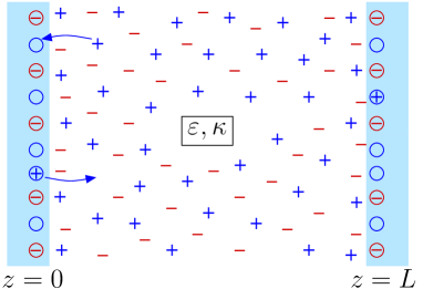
Figure 1: Schematic illustration of two chemically identical surfaces separated by a distance $L$ and interacting electrostatically across an electrolyte solution with permittivity $\varepsilon$ and inverse Debye length $\kappa$. Both surfaces contain fixed negative surface charges $\ominus$ and sites $\fullmoon$ where cations (+) from the solution can attach or from which adsorbed cations $\oplus$ can detach.

II Model

There are several models present in the literature, based on the surface free energy implementation of the charge regulation process, describing, e.g., of mineral surfaces Hie_89_1 ; Hie_89_2 ; Kos05 or lipid membranes Har06 ; Mar16 , and here we follow the latter. We consider two charge-regulated, chemically identical planar surfaces situated perpendicular to a $z$-axis at positions $z=0$ and $L$ with an electrolyte solution in between (see Fig. 1). Each surface contains a fixed number of negative charges per surface area, $N$, and a number of neutral sites per surface area, $\Theta N$, where adsorption and desorption of cations can take place, leading to charge regulation of the surfaces. The charge density on a surface is then given by $\sigma=-Ne+Ne\eta\Theta$ with $e>0$ being the elementary charge and $\eta$ denoting the fraction of occupied sites on a surface. Since by construction $\eta\in[0,1]$, for $\Theta=2$, i.e., when there are twice as many sites present compared to fixed negative charges Nat15 , the charge density varies within a symmetric interval $\sigma\in[-Ne,Ne]$. The area per site is $a^{2}=1/(\Theta N)$, and we define the dimensionless charge density as

$$\sigma^{*}=\frac{a^{2}\sigma}{e}=\eta-\frac{1}{\Theta}.$$ (1)

The parameter $\eta$ and therefore $\sigma^{*}$ are assumed to be uniform over the surface. The electrolyte is considered to be a structureless, linear dielectric medium with permittivity $\varepsilon=\varepsilon_{r}\varepsilon_{0}$, where $\varepsilon_{0}$ is the permittivity of the vacuum and $\varepsilon_{r}$ is the relative permittivity. The solute is a monovalent salt of bulk ionic strength $I$ and the corresponding Debye screening length is given by $\kappa^{-1}=\sqrt{\varepsilon/(2\beta e^{2}I)}$ with the inverse thermal energy $\beta=1/(k_{B}T)$.

III Density functional theory

Considering the bulk of the electrolyte as a reservoir for the ions, treating them as point-like particles, and ignoring ion-ion correlations within a mean-field formalism, the grand potential $\Omega\left[\sigma^{*},n_{\pm}\right]$ can be written in terms of the number density profiles of ions $n_{\pm}\left(\mathbf{r}\right)$ and surface charge density $\sigma^{*}(\mathbf{r})$. The Euler-Lagrange equation minimizing this grand potential with respect to $n_{\pm}$ leads to the PB equation $\nabla^{2}\psi=\kappa^{2}\sinh\psi$ subjected to Neumann boundary conditions at the surfaces set by $\sigma^{*}$. Here $\psi(\mathbf{r})$ is the dimensionless electrostatic potential expressed in units of $\beta e$. Hence the equilibrium ion number density profiles $n_{\pm}\left[\sigma^{*}\right]$ and the equilibrium electrostatic potential $\psi\left[\sigma^{*}\right]$ are functionals of $\sigma^{*}$. Inserting $n_{\pm}\left[\sigma^{*}\right]$ in the expression for $\Omega\left[\sigma^{*},n_{\pm}\right]$ one obtains the total grand potential functional in terms of the surface charge density profile $\sigma^{*}$. In the present work the surface charge density profile $\sigma^{*}$ is assumed to be laterally uniform on each surface, i.e., $\sigma^{*}\left(\mathbf{r}\right)$ and consequently, $\eta\left(\mathbf{r}\right)$ may depend at most on $z=0,L$. As a result, the electrostatic potential $\psi$ also depends on the $z$-coordinate only. With these, $\widetilde{\Omega}\left[\sigma^{*}\right]$, which is the grand potential functional $\Omega\left[\sigma^{*}\right]$ per unit surface area, corresponding to our system is given by

$$\beta\widetilde{\Omega}\left[\sigma^{*}\right]= \frac{-\varepsilon}{\beta e^{2}}\int\limits_{0}^{L}dz\Bigg{[}\kappa^{2}\cosh\left(\psi\left(z,\left[\sigma^{*}\right]\right)\right)+\frac{1}{2}\left(\psi^{\prime}\left(z,\left[\sigma^{*}\right]\right)\right)^{2}\Bigg{]}$$

$$+\frac{1}{a^{2}}\sum\limits_{z=0,L}\Bigg{[}\sigma^{*}\left(z\right)\psi\left(z,\left[\sigma^{*}\right]\right)$$

$$-\alpha\eta\left(z\right)-\frac{\chi}{2}\eta\left(z\right)^{2}$$

$$+\eta\left(z\right)\ln\eta\left(z\right)+\left(1-\eta\left(z\right)\right)\ln\left(1-\eta\left(z\right)\right)\Bigg{]},$$ (2)

where $\psi^{\prime}\equiv\partial_{z}\psi$ and $\eta\left(z\right)=\sigma^{*}\left(z\right)+1/\Theta$ according to Eq. (1). The first line of Eq. (2) represents the volume electrostatic contribution to the grand potential and is identical to the standard PB form Saf18 . The second line represents the standard surface electrostatic energy of the adsorbed charges. The third line describes the non-electrostatic free energy penalty of adsorption per ion, $\alpha$, being linear in the fraction of occupied sites on a surface, as well as the change in the non-electrostatic interactions between the ions upon adsorption, formalized by the Flory-Huggins parameter $\chi$ and therefore quadratic in the fraction of occupied sites on a surface Har06 ; Mar16 . The last line in Eq. (2) is describing the mixing entropy of the adsorbed cations at neutral sites with probability $\eta\left(z\right)$. The values of $\alpha$ and $\chi$ are related to the specific chemistry of the two surfaces and the dissociation processes responsible for the charge regulation. In the case of charge-regulation by $\text{H}^{+}$ dissociation, $\alpha\approx\left(\text{pK}-\text{pH}\right)\ln 10$ can be tuned by changing the pH of the solution; pK corresponds to the equilibrium constant of the surface dissociation process Saf18 . Increasing $\alpha$, then promotes a favorable adsorption of protons onto the surface, while an increase in $\chi$ lowers the free energy of the system, so that an already adsorbed proton prefers the filling of a neighboring site. The dimensionless parameters $\alpha$ and $\chi$ are phenomenological and their values are obtained from fitting the experimental data. Such an extension of the original charge regulation model by Ninham and Parsegian Nin71 was invoked in order to explain the details of an experimentally observed lamellar-lamellar phase transition in charged surfactant systems Dub98 ; Har06 . With both surfaces assumed to be chemically identical, and described by the same set $(\alpha,\chi)$ of phenomenological parameters, the equilibrium values for $\sigma^{*}\left(z\right)$ at the two surfaces are then determined by minimizing $\beta\widetilde{\Omega}\left[\sigma^{*}\right]$ in Eq. (2) with respect to $\sigma^{*}$.

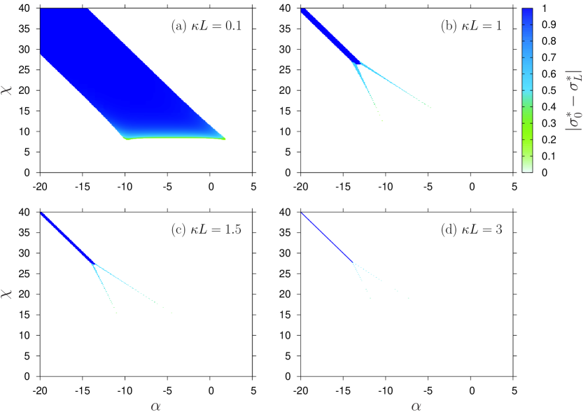
Figure 2: Absolute value of the difference of the dimensionless charge densities $\sigma^{*}=\frac{a^{2}\sigma}{e}\in\left[-\frac{1}{2},\frac{1}{2}\right]$ at the two surfaces, $\left|\sigma^{*}_{0}-\sigma^{*}_{L}\right|$, as function of $\alpha$ and $\chi$ (see Eq. (2)) for (a) $\kappa L=0.1$, (b) $1$, (c) $1.5$, and (d) $3$. The white regions in each figure correspond to a symmetric situation where $\sigma^{*}_{0}=\sigma^{*}_{L}$ whereas in the colored regions the equilibrium values of $\sigma^{*}_{0}$ and $\sigma^{*}_{L}$ differ from one another.

IV Results and discussion

As mentioned earlier, the surface charge density profile $\sigma^{*}$ is laterally uniform on each surface, i.e., it may depend at most on $z=0,L$. In the following we use the notation $\sigma^{*}(0)=\sigma^{*}_{0}$ and $\sigma^{*}(L)=\sigma^{*}_{L}$. Both $\eta(0)$ and $\eta(L)$ can vary in the interval $[0,1]$ and for $\Theta=2$, which is the case considered here, this corresponds to $\sigma^{*}\in\left[-\frac{1}{2},\frac{1}{2}\right]$ on each surface. Figure 2 shows the variation of the quantity $\left|\sigma^{*}_{0}-\sigma^{*}_{L}\right|$ with $\alpha$ and $\chi$ for gradually increasing separation $\kappa L$ between the surfaces. The parameters are varied in the intervals $\alpha\in[-20,5]$ and $\chi\in[0,40]$, which can be considered as within the experimentally relevant regime Har06 . Moreover realistic values $T=300\,\mathrm{K}$, $\varepsilon_{r}=80$ (water), and $a=1\,\mathrm{nm}$ are used. Note that under these conditions $\kappa^{-1}\approx 10\,\mathrm{nm}$ for an ionic strength $I=1\,\mathrm{mM}$. However, ionic strengths down to $\approx 0.01\,\mathrm{mM}$ are used for experimental studies in the present context Isr11 .

First, we consider the case $\kappa L=1$. As shown by Fig. 2(b), $\sigma^{*}_{0}$ and $\sigma^{*}_{L}$ are the same over a broad region (indicated by white) but not everywhere. In the dark blue region, the charge asymmetry is the highest and close to unity, implying that the two surfaces are oppositely charged. The line $\chi=-2\alpha$ passes through the middle of this region. Along this line, the solution is $\sigma^{*}_{0}=\sigma^{*}_{L}=0$ for $\alpha>\alpha_{0}$ ($\approx-13.2$ in this case) and for $\alpha\lesssim\alpha_{0}$ the dark blue region appears. For $\alpha\gtrsim\alpha_{0}$ there are two more regions (one below the line $\chi=-2\alpha$ and one above) where the charge asymmetry is present albeit with a lower contrast $\left|\sigma^{*}_{0}-\sigma^{*}_{L}\right|$. These two tails (light blue or greenish) are not inter-connected but with decreasing $\alpha$ they thicken, come close to each other, and finally merge with the dark blue region. The charge contrast in each of these two regions increases with decreasing $\alpha$. Below the dark blue region and the lower tail, the equilibrium states are symmetric with $\sigma^{*}_{0}=\sigma^{*}_{L}\gtrsim-\frac{1}{2}$ whereas above the dark blue region and the upper tail, they are symmetric with $\sigma^{*}_{0}=\sigma^{*}_{L}\lesssim\frac{1}{2}$. In between the two tails the states are $\sigma^{*}_{0}=\sigma^{*}_{L}\approx 0$. In other words, $(\sigma^{*}_{0},\sigma^{*}_{L})$ changes from $(\gtrsim-\frac{1}{2},\gtrsim-\frac{1}{2})$ to $(\lesssim\frac{1}{2},\lesssim\frac{1}{2})$ across the dark blue region, from $(\gtrsim-\frac{1}{2},\gtrsim-\frac{1}{2})$ to $(\approx 0,\approx 0)$ across the lower tail, and from $(\approx 0,\approx 0)$ to $(\lesssim\frac{1}{2},\lesssim\frac{1}{2})$ across the upper tail.

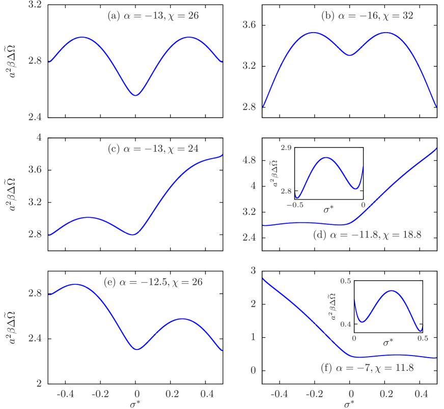
Figure 3: Variation of $\Delta\widetilde{\Omega}(\sigma^{*})$ (see Eq. (21) in the Appendix), which is obtained after subtracting the bulk contribution from the grand potential functional $\widetilde{\Omega}$ per unit surface area for a system consisting of a single charge-regulated surface in contact with an electrolyte and expressed in the units of $1/\left(a^{2}\beta\right)$, as function of $\sigma^{*}$ for different combinations of the parameters $\alpha$ and $\chi$. In all cases $\lambda=\beta e^{2}/\left(4\varepsilon\kappa a^{2}\right)\approx 21.3$ is used.

With decreasing separation $L$ between the two surfaces, the dark blue region in Fig. 2 broadens and starts to dominate over the tails, making them hardly visible (see Fig. 2(a)). With increasing separation all the regions shrink (see Figs. 2(c) and 2(d)) and the tails become increasingly difficult to be resolved numerically. In Fig. 2 both the interaction parameters $\alpha$ and $\chi$ are sampled with a tenth of the thermal energy $k_{B}T=1/\beta$ because ion adsorption is governed by a competition with the bulk solvation free energy, which can usually be measured within a similar accuracy Mar83 ; Ine94 . However, the dark blue region seems to be very stable and it remains present even at $\kappa L=10$. Upon increasing $\kappa L$ from $0.1$ to $3$ both $\alpha_{0}$ and the width of the dark blue region decrease relatively fast, whereas for $\kappa L$ between $3$ and $10$, they hardly change.

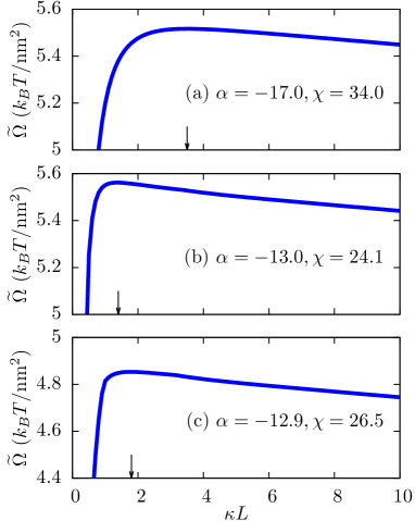
Figure 4: Variation of the effective interaction potential $\widetilde{\Omega}$ per unit surface area between two charge-regulated surfaces in the units of $k_{B}T/\mathrm{nm}^{2}$ as function of the scaled separation $\kappa L$ for three different state points in Fig. 2(b) from (a) the dark blue region, (b) the lower tail and (c) the upper tail. As shown by the plots, the interaction energy increases initially, shows a maximum, and ultimately decreases monotonically. The initial increase in the interaction energy corresponds to a negative effective force at short distances $L$, implying that the interaction is attractive there. The value of $\kappa L$ at the maximum of $\widetilde{\Omega}$ is indicated by arrows. As expected, the attraction in the dark blue region of Fig. 2 is stronger than in the other colored regions due to a larger contrast in the surface charge densities.

In order to explain these findings we consider a single surface in contact with an electrolyte. This problem is analytically solvable and the solution shows that on the line $\chi=-2\alpha$, there are two equally deep (local) minima of the grand potential $\Omega(\sigma^{*})$ at $\sigma^{*}_{1}$ and $\sigma^{*}_{2}=-\sigma^{*}_{1}$ (see the Appendix). For $\alpha\gtrsim-14$, $\sigma^{*}=0$ corresponds to the single global minimum of the grand potential; see Fig. 3(a). However, for $\alpha\lesssim-14$, the global minimum shifts to states with $\sigma^{*}_{1}\gtrsim-\frac{1}{2}$ and $\sigma^{*}_{2}=-\sigma^{*}_{1}\lesssim\frac{1}{2}$; see Fig. 3(b). For $\alpha\lesssim-14$, in the presence of a second surface, one surface acquires the charge density $\sigma^{*}=\sigma^{*}_{1}$ and the other $\sigma^{*}=\sigma^{*}_{2}=-\sigma^{*}_{1}$ because the electrostatic attraction of two oppositely charged surfaces leads to a decrease of the grand potential of the system. Similarly, the one-surface problem shows equally deep global minima of $\Omega(\sigma^{*})$ at $\sigma^{*}\gtrsim-\frac{1}{2}$ and $\sigma^{*}\lesssim 0$ for points in the upper part of the lower tail of Fig. 2(b) (e.g., see Fig. 3(c)). A second surface leads to charge densities of $\sigma^{*}\gtrsim-\frac{1}{2}$ on one surface and of $\sigma^{*}\gtrsim 0$ on the other such that the free energy cost in going upward the curve in Fig. 3(c) is balanced by a reduction of the free energy due to electrostatic attraction. As we go down the lower tail of Fig. 2(b), the one-surface problem shows two unequally deep minima at $\sigma^{*}\gtrsim-\frac{1}{2}$ and $\sigma^{*}\lesssim 0$ for these points; see Fig. 3(d). Although for a single surface the minimum at $\sigma^{*}\gtrsim-\frac{1}{2}$ is slightly deeper than the one at $\sigma^{*}\lesssim 0$, the combination $\sigma^{*}_{0}=\sigma^{*}_{L}\gtrsim-\frac{1}{2}$ for two surfaces would be too expensive due to strong electrostatic repulsion and $\sigma^{*}_{0}=\sigma^{*}_{L}\lesssim 0$ is also a state of higher free energy. The balance for two surfaces is obtained for the combination $(\gtrsim-\frac{1}{2},\lesssim 0)$ by avoiding the repulsive interaction energy. As is shown in Figs. 3(e) and (f), a similar phenomenon occurs for the upper tail in Fig. 2(b) except for the fact that there the equilibrium states are at $\sigma^{*}\gtrsim 0$ and $\lesssim\frac{1}{2}$. With increasing separation $\kappa L$, the regions with charge asymmetry shrink because of a weaker electrostatic interaction due to screening.

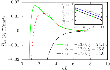
Figure 5: Electrostatic part $\widetilde{\Omega}_{\text{el}}$ of the effective interaction potential $\widetilde{\Omega}$ per unit surface area between two charge-regulated surfaces in units of $k_{B}T/\mathrm{nm}^{2}$ as function of the scaled separation $\kappa L$ for three different state points as in Fig. 4. For $\alpha=-17.0$ and $\chi=34.0$, the interaction is attractive everywhere implied by the opposite signs of the charge densities at the two surfaces. For the other two cases, the electrostatic interaction energies increase initially, show a maximum, and then decay to zero. Both the curves show kinks within the repulsive part of the interaction which are related to the discontinuities of the surface charge densities as functions of the wall separation $\kappa L$ (see Fig. 2). As expected, the interaction decays exponentially to zero which is confirmed by the semi-logarithmic plot in the inset.

Once $\sigma^{*}(\mathbf{r})$ is known, the grand potential per unit surface area of the system can be obtained by evaluating $\widetilde{\Omega}\left[\sigma^{*}\right]$; see Eq. (2). The dependence of $\widetilde{\Omega}$ as function of the separation $\kappa L$ describes an effective interaction potential between the surfaces and is shown in Fig. 4 for different combinations of the parameters $\alpha$ and $\chi$. In each case, $\widetilde{\Omega}$ increases initially with increasing $\kappa L$ and shows a maximum at some finite separation, typically well above the molecular length scale. Upon increasing $\kappa L$ further, the electrostatic interaction vanishes exponentially $\sim\exp(-\kappa L)$ (see Fig. 5) and the osmotic (or entropic) contribution ($=-2IL/\beta\sim L$) of the ions to $\widetilde{\Omega}$ dominates. The effective force per unit surface area $-\partial\widetilde{\Omega}/\partial L$ is negative up to the distance $L$ of the maximum in Fig. 4 and therefore, the interaction is attractive. This implies that the electrostatic attraction is sufficiently strong to overcome the repulsive osmotic pressure. At larger separations, however, the electrostatic interaction weakens and in the limit $L\rightarrow\infty$, the effective force per unit surface area equals the constant osmotic pressure $2I/\beta$. The occurrence of the maximum in Fig. 4(a) at a larger separation compared to the cases in Fig. 4(b) and (c) is related to enhanced electrostatic interactions due to the stronger asymmetry in the surface charge densities. Note that an effective interaction potential is a mesoscopic concept, which incorporates the energy and entropy balance of all microscopic degrees of freedom, e.g., the surface charge densities and the ion number density profiles, by minimization of the microscopic grand potential under the constraint of fixed mesoscopic degrees of freedom, e.g., the wall separation. In an even more microscopic (atomistic) approach, one could attempt to replace the parameters $\alpha$ and $\chi$ in favor of free energy contributions of the corresponding processes. In that sense an effective interaction energy always contains both energetic and entropic contributions.

The electrostatic part $\widetilde{\Omega}_{\text{el}}$ of the total interaction energy $\widetilde{\Omega}$ after subtracting the ideal osmotic (or entropic) contribution ($=-2IL/\beta\sim L$) of the ions and the surface tensions acting at the two solid-liquid interfaces, is shown as a function of the separation $\kappa L$ in Fig. 5 for the same values of the $\alpha$ and the $\chi$ parameters as in Fig. 4. For $\alpha=-17.0$ and $\chi=34.0$, which is a point on the line $\chi=-2\alpha$ in Fig. 2, the interaction is attractive due to the opposite charge densities at the two surfaces everywhere within the range of $\kappa L$ shown here. For the other two cases, the interactions are attractive at short distances $\kappa L$ and they become repulsive with increasing separation. These two curves show kinks corresponding to the discontinuities of the surface charge densities as functions of the wall separation $\kappa L$ (see Fig. 2). For example, if one considers the curve corresponding to $\alpha=-13.0$ and $\chi=24.1$, the two surfaces are oppositely charged up to $\kappa L\approx 1.5$, then, from $\kappa L\approx 1.5$ to $\kappa L\approx 1.9$, the two surfaces carry equal charge densities ($\sigma^{*}_{0}=\sigma^{*}_{L}\lesssim\frac{1}{2}$), from $\kappa L\approx 1.9$ to $\kappa L\approx 3.4$ the surfaces adopt charge densities which are different in magnitude but have equal signs ($\sigma^{*}_{0}\approx 0$, $\sigma^{*}_{L}\lesssim\frac{1}{2}$), and finally, beyond $\kappa L\approx 3.4$, both surfaces become equally charged ($\sigma^{*}_{0}=\sigma^{*}_{L}\approx 0$). A similar phenomenon occurs for $\alpha=-12.9$ and $\chi=26.5$ where the interaction changes from attractive to repulsive at $\kappa L\approx 2.9$, and at $\kappa L\approx 3.2$ the charge densities at the two surfaces become equal. As expected, at large separations, the electrostatic interaction in all cases decay exponentially $\sim\exp(-\kappa L)$; see the inset of Fig. 5. Please note that the equilibrium states are characterized by a minimum of the total interaction potential $\widetilde{\Omega}$ as function of the wall separation $L$. As $\widetilde{\Omega}(L)$ corresponds to the minimum of the grand potential functional $\Omega\left[\sigma^{*},n_{\pm}\right]$ under the constraint of a fixed wall separation $L$, it is necessarily continuous with respect to $L$, but its derivatives with respect to $L$ may be discontinuous at first-order phase transitions. In the present work no first-order bulk phase transitions are considered but the observed spontaneous symmetry breaking of the surface charge densities corresponds to first-order surface phase transitions. Hence, kinks can occur only in the surface contribution $\widetilde{\Omega}_{\text{el}}(L)$, and they are hardly visible in the total interaction $\widetilde{\Omega}(L)$ (note the widely different scales in Figs. 4 and 5).

The inter-surface force is usually measured by using a surface forces apparatus (SFA), atomic force microscopy (AFM), or optical tweezers Isr11 ; Tre17 . In order to observe the anomalous attraction discussed in the preceding paragraph for a surface with an appropriate charge regulation behavior, one can either fix the distance between the surfaces and change the ionic strength of the solution or fix the ionic strength and vary the separation between the surfaces. For relatively small separations compared to the Debye length, $L\lesssim 1/\kappa$, the system is expected to exhibit a broad parameter range of surface charge asymmetry (see, e.g., the colored region in Fig. 2(a)). Charge asymmetry is also present for larger separations $L$, but the corresponding parameter range is smaller and more difficult to find (see Fig. 2). In order to avoid possible additional effects occurring at short separations $L$ in a real experimental setup, it is advisable to use low ionic strengths, i.e., large Debye lengths $1/\kappa$. For example, $I=0.1\,\mathrm{mM}$ in water leads to $1/\kappa\approx 30\,\mathrm{nm}$, so that $\kappa L\approx 0.1$ for a separation length $L\approx 3\,\mathrm{nm}$, which is much larger than molecular dimensions and, therefore, a mean-field-like theory as the one presented here is expected to work well Tre17 . Moreover, it is not necessary to go to such small values of $\kappa L$: between $\kappa L=0.1$ and $1$ (e.g., $\kappa L=0.5$), one can expect to have a sufficiently broad parameter range of surface charge asymmetry (see the colored regions in Fig. 2). Possible candidates for the type of surfaces described here are biomolecules like lipids or proteins Isr11 or solid colloidal particles (e.g., made of silica) grafted with particular surface groups (e.g., $-\text{NH}_{2}$ or $-\text{COOH}$) (see Refs. Sol09 ; Yua17 ). The parameter $\chi$ can be adjusted by means of an appropriate arrangement and density of surface groups. On the other hand, the parameter $\alpha$ can be tuned by changing counterion concentration, e.g., the pH, in the solvent. As mentioned earlier, the parameters $\alpha$ and $\chi$ can be obtained, e.g., by fitting experimentally measured profiles of the effective force. For example, for the synthetic cationic double-chain surfactant didodecyldimethylammonium ($\text{DDA}^{+}$) the values $\alpha=-7.4,\chi=14.75$ for bromide ($\text{Br}^{-}$) and $\alpha=-3.4,\chi=14.75$ for chloride ($\text{Cl}^{-}$) counterions have been obtained in Ref. Har06 . This demonstrates that the parameter ranges for $\alpha$ and $\chi$, for which surface charge asymmetry is predicted here, are experimentally accessible, in particular in the case of low ionic strengths.

We finish our discussion by briefly commenting on the importance of the possible electrostatic attraction due to surface charge asymmetry in comparison with the van der Waals (vdW) attraction present in the system. The vdW interaction is usually estimated in terms of the Hamaker coefficient Ham37 . For a pair of parallel planar silica surfaces interacting across water, the Hamaker coefficient is $A\approx 4.8\times 10^{-21}\,\mathrm{J}$ (see Ref. Ber97 ), so that the vdW attraction energy per unit surface area $-A/\left(12\pi L^{2}\right)\approx 0.03\,k_{B}T/\mathrm{nm^{2}}$ for $L=1\,\mathrm{nm}$, which corresponds roughly to the thickness of the lines in Fig. 4. Hence the vdW interaction is qualitatively and quantitatively irrelevant for the effective interaction potentials considered in Fig. 4. The same can be expected for biological molecules, where the Hamaker coefficients are typically similar or smaller than $1\,k_{B}T$ (see Ref. Lec01 ).

It is important to note that our findings are not restricted to the case $\Theta=2$. For an asymmetric charge interval corresponding to $\Theta\neq 2$, the colored regions of Fig. 2 shift in the $\alpha$-$\chi$ plane but the qualitative features remain the same. In fact, we obtain asymmetric equilibrium states $\sigma^{*}_{0}\not=\sigma^{*}_{L}$ even for $\Theta=1$, where both surfaces can acquire only negative charges or remain uncharged; there the origin of asymmetry is similar to the greenish regions in Fig. 2.

V Conclusions

In conclusion, our results clearly indicate that chemically identical charge-regulated surfaces in an electrolyte are not necessarily equally charged and need not repel each other. Even if the surfaces are equally charged at larger separations, their symmetry can become spontaneously broken with decreasing inter-surface distance and they can assume charge densities differing in magnitude as well as in sign. At short separations, but well-above the molecular scale, the resulting electrostatic attraction dominates over the repulsive osmotic (or entropic) pressure due to the ions and the vdW attraction between the surfaces. These findings contradict one of the fundamental assumptions commonly made in the application of the PB theory to chemically identical surfaces and puts it into an entirely new perspective. Since charge regulation is prevalent in most synthetic as well as natural colloids, including biomolecules, our findings are indeed expected to be relevant for a wide range of systems.

Appendix A Single plate in contact with an electrolyte

A.1 Density functional

Let us consider a single charge-regulated wall placed at $z=0$ in contact with an electrolyte solution of bulk ionic strength $I$ and spanning the space $z>0$. The charge density at the wall is denoted by $\sigma$ and the dimensionless charge density is given by

$$\sigma^{*}=\frac{a^{2}\sigma}{e}=\eta-\frac{1}{\Theta}.$$ (3)

Please note that all variables used here and in the remainder have the same meaning as defined in the main text. After subtracting the bulk contribution from the grand potential functional $\Omega$ corresponding to Eq. (2) of the main text and afterwards dividing by the surface area $\mathcal{A}$ of the wall one obtains

$$\frac{\beta\Delta\Omega\left(\sigma^{*}\right)}{\mathcal{A}}= -\int\limits_{0}^{\infty}dz\Bigg{[}2I\left(\cosh\left(\psi\left(z\right)\right)-1\right)+\frac{\varepsilon}{2\beta e^{2}}\left(\psi^{\prime}\left(z\right)\right)^{2}\Bigg{]}+\frac{\sigma^{*}\psi\left(0\right)}{a^{2}}$$

$$+\frac{1}{a^{2}}\left(-\alpha\eta-\frac{\chi}{2}\eta^{2}+\eta\ln\eta+\left(1-\eta\right)\ln\left(1-\eta\right)\right),$$ (4)

where the dimensionless electrostatic potential $\psi$ satisfies the PB equation

$$\psi^{\prime\prime}\left(z\right)=\kappa^{2}\sinh\left(\psi\left(z\right)\right)$$ (5)

subjected to the Dirichlet boundary condition $\psi(\infty)=0$ and to the Neumann boundary condition

$$\psi^{\prime}(0)=-\frac{\beta e\sigma}{\varepsilon}=-\frac{\beta e^{2}}{\varepsilon a^{2}}\left(\eta-\frac{1}{\Theta}\right)=-\frac{\beta e^{2}\sigma^{*}}{\varepsilon a^{2}}.$$ (6)

As usual $\psi^{\prime}$ and $\psi^{\prime\prime}$ denote single and double derivatives with respect to $z$, respectively, and $\eta=\sigma^{*}+\frac{1}{\Theta}$ according to Eq. (3).

A.2 Grahame equation

Multiplying both sides of Eq. (5) by $\psi^{\prime}$ one obtains

$$\psi^{\prime}\psi^{\prime\prime}=\kappa^{2}\sinh\left(\psi\right)\psi^{\prime},$$

which can be rewritten as

$$\frac{1}{2}\left(\left(\psi^{\prime}\right)^{2}\right)^{\prime}=\kappa^{2}\left(\cosh\left(\psi\right)\right)^{\prime}.$$ (7)

Integrating Eq. (7) with respect to $z$ and using $\psi\left(\infty\right)=\psi^{\prime}\left(\infty\right)=0$ gives

$$\frac{1}{2}\left(\psi^{\prime}\right)^{2}=\kappa^{2}\left(\cosh\left(\psi\right)-1\right),$$ (8)

which leads to

$$2I\left(\cosh\left(\psi\right)-1\right)=\frac{\varepsilon}{2\beta e^{2}}\left(\psi^{\prime}\right)^{2}.$$ (9)

For $z=0$, i.e., at the wall, Eq. (8) gives the Grahame equation Gra47

$$\kappa^{2}\left(\cosh\left(\psi(0)\right)-1\right)=\frac{1}{2}\left(\psi^{\prime}(0)\right)^{2}=\frac{\beta^{2}e^{2}\sigma^{2}}{2\varepsilon^{2}},$$ (10)

and therefore,

$$\psi(0)=\mathrm{sign}\left(\sigma\right)\operatorname{arcosh}\left(1+\frac{\beta^{2}e^{2}\sigma^{2}}{2\varepsilon^{2}\kappa^{2}}\right).$$ (11)

The sign of $\sigma$ and $\sigma^{*}$ are the same according to Eq. (3) and for brevity we define the dimensionless parameter $\lambda=\frac{\beta e^{2}}{4\varepsilon\kappa a^{2}}$. With these, Eq. (11) can be rewritten as

$$\psi(0)=\mathrm{sign}\left(\sigma^{*}\right)\operatorname{arcosh}\left(1+8\lambda^{2}\left(\sigma^{*}\right)^{2}\right).$$ (12)

A.3 Electrostatic potential

The PB equation for our setup is analytically solvable and its solution is well know Hun89 ; Rus89 :

$$\psi(z)=4\operatorname{artanh}\left(\gamma\exp\left(-\kappa z\right)\right);~{}~{}~{}~{}~{}\gamma=\tanh\left(\frac{\psi(0)}{4}\right).$$ (13)

Taking the derivative with respect to $z$, one obtains

$$\psi^{\prime}(z)=-4\kappa\gamma\frac{\exp\left(-\kappa z\right)}{1-\gamma^{2}\exp\left(-2\kappa z\right)}.$$ (14)

Therefore,

$$\int\limits_{0}^{\infty}dz\left(\psi^{\prime}(z)\right)^{2} =16\kappa^{2}\gamma^{2}\int\limits_{0}^{\infty}dz\frac{\exp\left(-2\kappa z\right)}{\left(1-\gamma^{2}\exp\left(-2\kappa z\right)\right)^{2}}$$

$$=8\kappa\int\limits_{0}^{\infty}dz\frac{2\kappa\gamma^{2}\exp\left(-2\kappa z\right)}{\left(1-\gamma^{2}\exp\left(-2\kappa z\right)\right)^{2}}$$

$$=8\kappa\int\limits_{0}^{\infty}dz\left(\frac{d}{dz}\frac{-1}{1-\gamma^{2}\exp\left(-2\kappa z\right)}\right)$$

$$=8\kappa\left|\frac{-1}{1-\gamma^{2}\exp\left(-2\kappa z\right)}\right|_{z=0}^{\infty}$$

$$=8\kappa\left(-1+\frac{1}{1-\gamma^{2}}\right)$$

$$=\frac{8\kappa\gamma^{2}}{1-\gamma^{2}}.$$ (15)

The parameter $\gamma$ is determined by using the boundary condition relating the electric displacement vector to the charge density at the wall. Combining Eqs. (6) and (14), one obtains

$$\psi^{\prime}(0)=-4\kappa\frac{\gamma}{1-\gamma^{2}}=-\frac{\beta e\sigma}{\varepsilon},$$ (16)

which leads to

$$\frac{\gamma}{1-\gamma^{2}}=\frac{\beta e^{2}\sigma^{*}}{4\kappa\varepsilon a^{2}}=\lambda\sigma^{*}.$$ (17)

Solving Eq. (17) for $\gamma$ and inserting it in Eq. (15), one finally arrives at

$$\int\limits_{0}^{\infty}dz\left(\psi^{\prime}(z)\right)^{2}=4\kappa\left(-1+\sqrt{1+4\lambda^{2}\left(\sigma^{*}\right)^{2}}\right).$$ (18)

A.4 Grand potential

Using Eqs. (9) and (12) in Eq. (4), one can write

$$\frac{\beta\Delta\Omega\left(\sigma^{*}\right)}{\mathcal{A}}= -\int\limits_{0}^{\infty}dz\frac{\varepsilon}{\beta e^{2}}\left(\psi^{\prime}\right)^{2}+\frac{\sigma^{*}}{a^{2}}\mathrm{sign}\left(\sigma^{*}\right)\operatorname{arcosh}\left(1+8\lambda^{2}\left(\sigma^{*}\right)^{2}\right)$$

$$+\frac{1}{a^{2}}\left(-\alpha\eta-\frac{\chi}{2}\eta^{2}+\eta\ln\eta+\left(1-\eta\right)\ln\left(1-\eta\right)\right).$$ (19)

Further, using Eq. (18), Eq. (19) can be rewritten as

$$\frac{\beta\Delta\Omega\left(\sigma^{*}\right)}{\mathcal{A}}=\frac{1}{a^{2}}\Bigg{[} \frac{1}{\lambda}\left(1-\sqrt{1+4\lambda^{2}\left(\sigma^{*}\right)^{2}}\right)+\left|\sigma^{*}\right|\operatorname{arcosh}\left(1+8\lambda^{2}\left(\sigma^{*}\right)^{2}\right)$$

$$-\alpha\eta-\frac{\chi}{2}\eta^{2}+\eta\ln\eta+\left(1-\eta\right)\ln\left(1-\eta\right)\Bigg{]},$$ (20)

where the relation $\frac{4\kappa\varepsilon a^{2}}{\beta e^{2}}=\frac{1}{\lambda}$ is used.

A.5 Symmetric charge interval ($\Theta=2$)

As mentioned in the main text, $\Theta=2$ corresponds to a symmetric charge interval. For this case, $\eta=\sigma^{*}+\frac{1}{2}$ according to Eq. (3) and using this, Eq. (20) can be written as:

$$\beta\Delta\widetilde{\Omega}\left(\sigma^{*}\right)=\frac{1}{a^{2}}\Bigg{[} \frac{1}{\lambda}\left(1-\sqrt{1+4\lambda^{2}\left(\sigma^{*}\right)^{2}}\right)+\left|\sigma^{*}\right|\operatorname{arcosh}\left(1+8\lambda^{2}\left(\sigma^{*}\right)^{2}\right)$$

$$-\alpha\left(\frac{1}{2}+\sigma^{*}\right)-\frac{\chi}{2}\left(\frac{1}{2}+\sigma^{*}\right)^{2}$$

$$+\left(\frac{1}{2}+\sigma^{*}\right)\ln\left(\frac{1}{2}+\sigma^{*}\right)+\left(\frac{1}{2}-\sigma^{*}\right)\ln\left(\frac{1}{2}-\sigma^{*}\right)\Bigg{]},$$ (21)

where $\Delta\widetilde{\Omega}\left(\sigma^{*}\right)=\frac{\Delta\Omega\left(\sigma^{*}\right)}{\mathcal{A}}$ is the free energy per unit surface area. Clearly, $\beta\Delta\widetilde{\Omega}\left(\sigma^{*}\right)$ in Eq. (21) is symmetric about $\sigma^{*}=0$, i.e., $\beta\Delta\widetilde{\Omega}\left(-\sigma^{*}\right)=\beta\Delta\widetilde{\Omega}\left(\sigma^{*}\right)$, provided the condition

$$\left(2\alpha+\chi\right)\sigma^{*}=0$$ (22)

is fulfilled. According to this condition, on the line $\chi=-2\alpha$ two states with $\sigma^{*}_{1}$ and $\sigma^{*}_{2}=-\sigma^{*}_{1}$ correspond to the same value of $\beta\Delta\widetilde{\Omega}(\sigma^{*})$. Therefore, if a state with $\sigma^{*}_{1}$ corresponds to the global minimum of $\beta\Delta\widetilde{\Omega}(\sigma^{*})$, there will be another state with $\sigma^{*}_{2}=-\sigma^{*}_{1}$ with the same minimum, i.e., the two states with $\sigma^{*}_{1}$ and $\sigma^{*}_{2}$ coexist. As shown in Fig. 3 of the main text, for $\alpha\gtrsim-14$ and $\chi=-2\alpha$ the global minimum corresponds to $\sigma^{*}=-\sigma^{*}=0$ (see Fig. 3(a)) whereas for $\alpha\lesssim-14$, it shifts to $\sigma^{*}_{1}\gtrsim-\frac{1}{2}$ and $\sigma^{*}_{2}=-\sigma^{*}_{1}\lesssim\frac{1}{2}$ (see Fig. 3(b)).

References

- (1) T. Markovich, D. Andelman, and R. Podgornik, Charged Membranes: Poisson-Boltzmann theory, DLVO paradigm and beyond, Handbook of Lipid Membranes, Safynia, C., Raedler, J., Eds. (Taylor & Francis, 2018).
- (2) I. Popa, P. Sinha, M. Finessi, P. Maroni, G. Papastavrou, and M. Borkovec, Phys. Rev. Lett. 104, 228301 (2010).
- (3) M. Lund and B. Jönsson, Q. Rev. Biophys. 46, 265 (2013).
- (4) B. W. Ninham and V. A. Parsegian, J. Theor. Biol. 31, 405 (1971).
- (5) H. Diamant and D. Andelman, J. Phys. Chem. 100, 13732 (1996).
- (6) M. L. Henle, C. D. Santangelo, D. M. Patel, and P. A. Pincus, Europhys. Letts. 66 284 (2004).
- (7) G. S. Longo, M. Olvera de la Cruz, and I. Szleifer, ACS Nano 7, 2693 (2013).
- (8) A. C. Maggs and R. Podgornik, Europhys. Letts. 108 68003 (2014).
- (9) S. H. Behrens and M. Borkovec, J. Phys. Chem. B 103, 2918 (1999).
- (10) P. M. Biesheuvel, J. Colloid Interface Sci. 275, 514 (2004).
- (11) M. Borkovec and S. H. Behrens, J. Phys. Chem. B 112 10796 (2008).
- (12) G. Trefalt, S. H. Behrens, and M. Borkovec, Langmuir 32, 380 (2016).
- (13) D. Chan, T. W. Healy, and L. R. White, J. Chem. Soc., Faraday Trans. 72, 2844 (1976).
- (14) D. McCormack, S. L. Carnie, and D. Y. C. Chan, J. Colloid Interface Sci. 169, 177 (1995).
- (15) S. H. Behrens and M. Borkovec, Phys. Rev. E 60, 7040 (1999).
- (16) D. Y. C. Chan, T. W. Healy, T. Supasiti, and S. Usui, J. Colloid Interface Sci. 296, 150 (2006).
- (17) J. E. Sader and D. Y. C. Chan, J. Colloid Interface Sci. 213 268 (1999).
- (18) J. C. Neu, Phys. Rev. Lett. 82 1072 (1999).
- (19) E. Trizac and J.-L. Raimbault, Phys. Rev. E 60, 6530 (1999).
- (20) T. Hiemstra, W. H. V. Riemsdijk, and G. H. Bolt, J. Colloid Interface Sci. 133, 91 (1989).
- (21) T. Hiemstra, J. C. M. D. Wit, and W. H. V. Riemsdijk, J. Colloid Interface Sci. 133, 105 (1989).
- (22) M. Kosmulski, Langmuir 21, 7421 (2005).
- (23) D. Harries, R. Podgornik, V. A. Parsegian, E. Mar-Or, and D. Andelman, J. Chem. Phys. 124, 224702 (2006).
- (24) T. Markovich, D. Andelman, and R. Podgornik, Europhys. Letts. 113 26004 (2016).
- (25) N. Adžić and R. Podgornik, Phys. Rev. E 91 022715 (2015).
- (26) M. Dubois, Th. Zemb, N. Fuller, R. P. Rand, and V. A. Parsegian, J. Chem. Phys. 108, 7855 (1998).
- (27) J. N. Israelachvili, Intermolecular and Surface Forces (Academic Press, Amsterdam, 2011).
- (28) Y. Marcus, Pure Appl. Chem. 55, 977 (1983).
- (29) H. D. Inerowicz, W. Li, and I. Persson, J. Chem. Soc., Faraday Trans. 90, 2223 (1994).
- (30) G. Trefalt, T. Palberg, and M. Borkovec, Curr. Opin. Colloid Interface Sci. 27, 9 (2017).
- (31) N. Solin, L. Han, S. Che, and O. Terasaki, Catal. Commun. 10, 1386 (2009).
- (32) L. Yuan, L. Chen, X. Chen, R. Liu, and G. Ge, Langmuir 33, 8724 (2017).
- (33) H. C. Hamaker, Physica 4, 1058 (1937).
- (34) L. Bergström, Adv. Colloid Interface Sci. 70, 125 (1997).
- (35) D. Leckband and J. Israelachvili, Q. Rev. of Biophys. 34, 105 (2001).
- (36) D. C. Grahame, Chem. Rev. 41, 441 (1947).
- (37) R. J. Hunter, Foundations of colloid science (Clarendon Press, Oxford, 1989).
- (38) W. B. Russel, D. A. Saville, W. R. Schowalter, Colloidal dispersions (Cambridge University Press, 1989).