Photon sector analysis of Super and Lorentz symmetry breaking: effective photon mass, bi-refringence and dissipation

Abstract

Within the Standard Model Extension (SME), we expand our previous findings on four classes of violations of Super-Symmetry (SuSy) and Lorentz Symmetry (LoSy), differing in the handedness of the Charge conjugation-Parity-Time reversal (CPT) symmetry and in whether considering the impact of photinos on photon propagation. The violations, occurring at the early universe high energies, show visible traces at present in the Dispersion Relations (DRs). For the CPT-odd classes ($V_{\mu}$ breaking vector) associated with the Carroll-Field-Jackiw (CFJ) model, the DRs and the Lagrangian show for the photon an effective mass, gauge invariant, proportional to $|{\vec{V}}|$. The group velocity exhibits a classic dependency on the inverse of the frequency squared. For the CPT-even classes ($k_{F}$ breaking tensor), when the photino is considered, the DRs display also a massive behaviour inversely proportional to a coefficient in the Lagrangian and to a term linearly dependent on $k_{F}$. All DRs display an angular dependence and lack LoSy invariance. In describing our results, we also point out the following properties: i) the appearance of complex or simply imaginary frequencies and super-luminal speeds and ii) the emergence of bi-refringence. Finally, we point out the circumstances for which SuSy and LoSy breakings, possibly in presence of an external field, lead to the non-conservation of the photon energy-momentum tensor. We do so for both CPT sectors.

1 Introduction, motivation and structure of the work

For the most part, we base our understanding of particle physics on the Standard Model (SM). The SM proposes the Lagrangian of particle physics and summarises three interactions among fundamental particles, accounting for electromagnetic (EM), weak and strong nuclear forces. The model has been completed theoretically in the mid seventies, and has found several experimental confirmations ever since. In 1995, the top quark was found Abetal95 ; in 2000, the tau neutrino was directly measured koetal00 . Last, but not least, in 2012 the most elusive particle, the Higgs Boson, was found Aad2015 . The associated Higgs field induces the spontaneous symmetry breaking mechanism, responsible for all the masses of the SM particles. Neutrinos and the photon remain massless, for they do not have a direct interaction with the Higgs field. Remarkably, massive neutrinos are not accounted for by the SM.

All ordinary hadronic and leptonic matter is made of Fermions, while Bosons are the interaction carriers in the SM. The force carrier for the electromagnetism is the photon. Strong nuclear interactions are mediated by eight gluons, massless but not free particles, described by Quantum Chromo-Dynamics (QCD). Instead, the $W^{+}$, $W^{-}$ and $Z$ massive Bosons, are the mediators of the weak interaction. The charge of the W-mediators has suggested that the EM and weak nuclear forces can be unified into a single interaction called electroweak interaction.

We finally notice that the photon is the only massless non-confined Boson; the reason for this must at least be questioned by fundamental physics.

SM considers all particles being massless, before the Higgs field intervenes. Of course, masslessness of particles would be in contrast with every day experience. In 1964, Higgs and others higgs1964 ; englertbrout1964 ; guralnikhagenkibble1964 came up with a mechanism that, thanks to the introduction of a new field - the Higgs field - is able to explain why the elementary particles in the spectrum of the SM, namely, the charged leptons and quarks, become massive. But the detected mass of the Higgs Boson is too light: in 2015 the ATLAS and CMS experiments showed that the Higgs Boson mass is $125.09\pm 0.32\$ GeV/c² Aad2015 . Between the GeV scale of the electroweak interactions and the Grand Unification Theory (GUT) scale ($10^{16}$ GeV), it is widely believed that new physics should appear at the TeV scale, which is now the experimental limit up to which the SM was tested Lykken2010 . Consequently, we need a fundamental theory that reproduces the phenomenology at the electroweak scale and, at the same time, accounts for effects beyond the TeV scale.

An interesting attempt to go beyond the SM is for sure Super-Symmetry (SuSy); see martin2016 for a review. This theory predicts the existence of new particles that are not included in the SM. The interaction between the Higgs and these new SuSy particles would cancel out some SM contributions to the Higgs Boson mass, ensuring its lightness. This is the solution to the so-called gauge hierarchy problem. The SM is assumed to be Lorentz Symmetry (LoSy) invariant. Anyway, it is reasonable to expect that this prediction is valid only up to certain energy scales kosteleckysamuel1989a ; kosteleckysamuel1989b ; kosteleckysamuel1989c ; kosteleckysamuel1991 ; kosteleckypotting1991 ; kosteleckypotting1995 ; kosteleckypotting1996 , beyond which a LoSy Violation (LSV) might occur. The LSV would take place following the condensation of tensor fields in the context of open Bosonic strings.

The aforementioned facts show that there are valid reasons to undertake an investigation of physics beyond the SM and also consider LSV. There is a general framework where we can test the low-energy manifestations of LSV, the so-called Standard Model Extension (SME) colladaykostelecky1997 ; colladaykostelecky1998 ; myerspospelov2003 ; liberati2013 . Its effective Lagrangian is given by the usual SM Lagrangian, modified by a combination of SM operators of any dimensionality contracted with Lorentz breaking tensors of suitable rank to get a scalar expression for the Lagrangian.

For the Charge conjugation-Parity-Time reversal (CPT) odd classes the breaking factor is the $V_{\mu}$ vector associated with the Carroll-Field-Jackiw (CFJ) model cafija90 , while for the CPT-even classes it is the $k_{F}$ tensor.

In this context, LSV has been thoroughly investigated phenomenologically. Studies include electron, photon, muon, meson, baryon, neutrino and Higgs sectors kosteleckyrussell2011 . Limits on the parameters associated to the breaking of relativistic covariance are set by quite a few experiments kosteleckyrussell2011 ; kosteleckytasson2009 ; baileykostelecky2004 . LSV has also been tested in the context of EM cavities and optical systems russell2005 ; phhumastvewa2001 ; bestwakola2000 ; huphmavest2003 ; mubrhepela2003 ; muhesapela2003 ; muller2005 . Also Fermionic models in presence of LSV have been proposed: spinless and/or neutral particles with a non-minimal coupling to a LSV background, magnetic properties in relation to Fermionic matter or gauge Bosons besifeor2011 ; bakkebelichsilva2011a ; bakkebelichsilva2011b ; bakkebelich2012 ; casanaferreirasantos2008a ; casanaferreirasantos2008b ; casanaferreiragomespinheiro2009a ; casanaferreiragomespinheiro2009b ; casanaferreirarodriguessilva2009 ; limabelichbakke2013 ; cvdshobe2014 ; hernaskibelich2014 .

More recently, fu-lehnert-2016 ; colladay-noordmans-potting-2017 present interesting results involving the electroweak sector of the SME.

Following colladaymcdonald2011 ; bergerkostelecky2002 ; falenape2012 ; bolokhovnibbelinkpospelov2005 ; katzshadmi2006 ; nibbelinkpospelov2005 ; redigolo2012 ; golenapeds2013 ; lenapeds2013 ; hnbedilesp2010 , LSV is stemmed from a more fundamental physics because it concerns higher energy levels of those obtained in particle accelerators. In Fig. 1, we show the energy scales at which the symmetries are supposed to break, referring to the model described in bebegahnle2015 . At Planck scale, $10^{19}$ GeV, all symmetries are exact, unless LoSy breaking occurs. This latter may intervene at a lower scale of $10^{17}$ GeV, but anyway above GUT. Between $10^{11}$ and $10^{19}$ GeV, we place the breaking of SuSy. In our analysis, we assume that the four cases of SuSy breaking occur only when LoSy has already being violated. Interestingly, at our energy levels, we can detect the reminiscences of these symmetry breakings.

Indeed, we adopt the point of view that the LSV background is part of a SuSy multiplet; see for instance bebegahnle2015 .

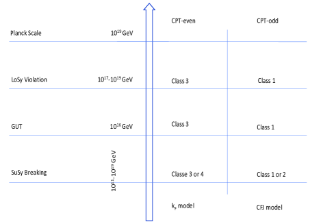
Figure 1: We show the energy scales at which the symmetries are supposed to break, referring to the model described in bebegahnle2015 . At Planck scale, $10^{19}$ GeV, all symmetries are exact, unless LoSy breaking occurs. This latter may intervene at a lower scale of $10^{17}$ GeV, but anyway above GUT. Between $10^{11}$ and $10^{19}$ GeV, we place the breaking of SuSy. In our analysis, we assume that the four cases of SuSy breaking occur only when LoSy has already being violated. Interestingly, at our energy levels, we can detect the reminiscences of these symmetry breakings.

Since gravitational wave astronomy is at its infancy, EM wave astronomy remains the main detecting tool for unveiling the universe. Thereby, testing the properties of the photons is essential to fundamental physics and astrophysics has just to interpret the universe accordingly.

A legitimate question addresses which mechanism could provide mass to the photon and thereby how the SM should be extended to accommodate such a conjecture. We have set up a possible scenario to reply to these two questions with a single answer.

Non-Maxwellian massive photon theories have been proposed over the course of the last century. If the photon is massive, propagation is affected in terms of group velocity and polarisation.

This work is structured as follows. In Sect. 2, we summarise, complement and detail the results obtained in our letter bodshnsp2017 , with some reminders to the appendix. Within the unique SME model, we consider four classes of models that exhibit LoSy and SuSy violations, varying in CPT handedness and in incorporating - or not - the effect of photino on the photon propagation. The violation occurs at very high energies, but we search for traces in the DRs visible at our energy scales. In the same Section, we confirm that a massive photon term emerges from the CPT-odd Lagrangian. We discover that a massive photon emerges also for the CPT-even sector when the photino is considered. We also point out when i) complex or simply imaginary frequencies and super-luminal speeds arise. In Sect. 3, we look for multi-fringence. In Sect. 4, we wonder if dissipation is conceivable for wave propagation in vacuum and find an affirmative answer. In Sect. 5, we propose our conclusions, discussion and perspectives. The appendix gives some auxiliary technical details.

1.1 Reminders and conventions

We shall encounter real frequencies sub- and luminal velocities but also imaginary and complex frequencies, and super-luminal velocities.

In this work, see the title, we intend photon mass as an effective mass. The photon is dressed of an effective mass, that we shall see, depends on the perturbation vector or tensor. Nevertheless, we are cautious in differentiating an effective from a real mass. The Higgs mechanism gives masses to the charged leptons and quarks, the W and Z bosons, while the composite hadrons (baryons and mesons), built up from the massive quarks, have most of their masses from the mechanism of Chiral Symmetry (Dynamical) Breaking (CSB). It would be epistemologically legitimate to consider such mechanisms as producing an effective mass to particles which, without such dressing mechanisms, would be otherwise massless. What is then real or effective? The feature of being frame dependent renders surely the concept of mass unusual, but still acceptable to our eyes, being the dimension indeed that of a mass.

We adopt natural units for which $c=\hbar=1/4\pi\epsilon_{0}=\mu=1$, unless otherwise stated. We adopt the metric signature as (+, -, -, -). Although more recent literature adopts $k_{AF}^{\mu}$ and $k_{F}^{\mu\nu\rho\sigma}$ for LSV vector and tensor, respectively, we drop the former in favour of $V^{\mu}$ for simplicity of notation especially when addressing time or space components and normalised units.

Finally, we omit to use the adjective angular, when addressing the angular frequency $\omega$.

1.2 Upper limits on $V_{\mu}$ vector and photon mass $m_{\gamma}$

Ground based experiments indicate that $|{\vec{V}}|$, the space components, must be smaller than $10^{-10}$ eV $=1.6\times 10^{-29}$ J from the bounds given by the energy shifts in the spectrum of the hydrogen atom gomesmalta2016 ; else smaller than $8\times 10^{-14}$ eV $=1,3\times 10^{-32}$ J from measurements of the rotation in the polarisation of light in resonant cavities gomesmalta2016 . The time component of $V_{\mu}$ is smaller than $10^{-16}$ eV $=1.6\times 10^{-35}$ J gomesmalta2016 Instead, astrophysical observations lead to $|{\vec{V}}|<10^{-34}$ eV $=1.6\times 10^{-53}$ J. We cannot refrain to remark that such estimate is equivalent to the Heisenberg limit ($\Delta m\Delta t>1$) on the smallest measurable energy or mass for a given time t, set equal to the Universe age. The actual Particle Data Group (PDG) limit on photon mass tanabashietal2018 refers to values obtained in Ryutov1997 ; Ryutov2007 of $10^{-54}$ kg or $5.6\times 10^{-19}$ eV/c², to be taken with some care, as motivated in retinospalliccivaivads2016 ; boelmasasgsp2016 ; boelmasasgsp2017 .

2 LSV and two classes of SuSy breaking for each CPT sector

We summarise and complement in this section the results obtained in bodshnsp2017 .

2.1 CPT-odd sector and the $V_{\mu}$ vector: classes 1 and 2

The CFJ proposition cafija90 introduced LSV by means of a Chern-Simons (CS) chernsimons1974 term in the Lagrangian that represents the EM interaction. It was conceived and developed outside any SuSy scenario. The works baetaetal2004 and later bebegahnle2015 framed the CFJ model in a SuSy scenario. The LSV is obtained through the breaking vector $V_{\mu}$, the observational limits of which are considered in the CFJ framework. For the origin, the microscopic justification was traced in the fundamental Fermionic condesates present in SuSy bebegahnle2015 . In other words, the Fermionic fields present in the in SuSy background may condensate (that is, take a vacuum expectation value), thereby inducing LSV.

In the following, the implications of the CS term on the propagation and DR of the photon are presented.

2.1.1 Class 1: CFJ model

The Lagrangian reads

$$L_{1}=-\frac{1}{4}F^{\mu\nu}F_{\mu\nu}-\frac{1}{2}\epsilon^{\mu\nu\sigma\rho}V_{\mu}A_{\nu}F_{\sigma\rho}~{}.$$ (3)

where $F_{\mu\nu}=\partial_{\mu}A_{\nu}-\partial_{\nu}A_{\mu}$ and $F^{\mu\nu}=\partial^{\mu}A^{\nu}-\partial^{\nu}A^{\mu}$ are the covariant and contravariant forms, respectively, of the EM tensor; $\epsilon^{\mu\nu\sigma\rho}$ is the contravariant form of the Levi-Civita pseudo-tensor, and $A_{\mu}$ the potential covariant four-vector.

We observe the coupling between the EM field and the breaking vector $V_{\mu}$. The Euler-Lagrange variational principle applied to Eq. (3) leads to

$$\vec{\nabla}\times\vec{B}+V_{0}\vec{B}-\vec{V}\times\vec{E}=\partial_{t}\vec{E}~{}.$$ (4)

where the three-vector $\vec{V}$ represents the space components of $V_{\mu}$, and $\vec{B}$ and $\vec{E}$ the magnetic and electric fields.

From the Fourier transformation of the curl of the electric field $(\vec{\nabla}\times\vec{E})$ equation, we obtain $\tilde{\vec{B}}$ in terms of $\tilde{\vec{E}}$, magnetic and electric field in Fourier domain, respectively

$$\vec{\tilde{B}}={\frac{\vec{k}}{\omega}}\times\vec{\tilde{E}}~{},$$ (5)

where the four-momentum is $k^{\mu}=\left(\omega,\vec{k}\right)$ and where $k^{2}=(\omega^{2}-{\bf k^{2}})$. Inserting Eq. (5) into the Fourier transform of Eq. (4), we get

$$\left(\omega^{2}-\vec{k}^{2}\right)\vec{\tilde{E}}+\left(\vec{k}\cdot\vec{\tilde{E}}\right)\vec{k}=i\left(V_{0}\vec{k}\times\vec{\tilde{E}}-\omega\vec{V}\times\vec{\tilde{E}}\right)~{}.$$ (6)

Equation (9) can be arranged in the form

$$R_{ij}\tilde{E}_{j}=0~{},$$ (7)

where $R_{ij}$ is the matrix

$$R_{ij}=i\vec{k}^{2}\delta_{ij}+ik_{i}k_{j}-V_{0}\epsilon_{ijk}k_{k}+\epsilon_{ijk}\omega V_{k}~{}.$$ (8)

Imposing $\mbox{det}~{}R_{ij}=0$, we derive the DR, Eq. (3) in bodshnsp2017 , known since the appearance of cafija90

$$\left(k^{\mu}k_{\mu}\right)^{2}+\left(V^{\mu}V_{\mu}\right)\left(k^{\nu}k_{\nu}\right)-\left(V^{\mu}k_{\mu}\right)^{2}=0~{}.$$ (9)

2.1.2 Class 2: Supersymmetrised CFJ model and SuSy breaking

We can study the effect of the photino on the photon propagation. For accounting for the effects of the photino, according to bebegahnle2015 , we have to work with the Lagrangian that follows below

$$L_{2}=-\frac{1}{4}F+\frac{1}{4}\epsilon^{\mu\nu\rho\sigma}V_{\mu}A_{\nu}F_{\rho\sigma}+\frac{1}{4}HF+M_{\mu\nu}F^{\mu\lambda}{F^{\nu}_{\lambda}}~{},$$ (10)

where $F=F_{\mu\nu}F^{\mu\nu}$; furthermore, $H$ is a scalar defined in bebegahnle2015 , the tensor $M_{\mu\nu}=\hat{M}_{\mu\nu}+{\displaystyle\frac{1}{4}}~{}\eta_{\mu\nu}M$, and $\hat{M}_{\mu\nu}$ depends on the background Fermionic condensate, originated by SuSy; $\hat{M}_{\mu\nu}$ is traceless, $M$ the trace of $M_{\mu\nu}$, and $\eta_{\mu\nu}$ the Minkowski metric. The Lagrangian, Eq. (10), is rewritten as bebegahnle2015

$$L_{2}=-\frac{1}{4}\left(1-H-M\right)F+\frac{1}{4}\epsilon^{\mu\nu\rho\sigma}V_{\mu}A_{\nu}F_{\rho\sigma}+\hat{M}_{\mu\nu}F^{\mu\lambda}F_{\lambda}^{\nu}~{}.$$ (11)

In bebegahn2013 it is shown that the DR is equivalent to Eq. (9), but for a rescaling of the breaking vector. The latter is obtained by integrating out the Fermionic SuSy partner, the photino. The following DR comes out (Eq. (6) in bodshnsp2017 )

$$\left(k^{\mu}k_{\mu}\right)^{2}+\frac{\left(V^{\mu}V_{\mu}\right)\left(k^{\nu}k_{\nu}\right)}{\left(1-H-M\right)^{2}}-\frac{\left(V^{\mu}k_{\mu}\right)^{2}}{\left(1-H-M\right)^{2}}=0~{}.$$ (12)

The background parameters are very small, being suppressed by powers of the Planck energy; they render the denominator in Eq. (12) close to unity, implying similar numerical outcomes for the two dispersion relations of Classes 1 and 2. Consequently, we shall derive and work with group velocities and time delays, for Classes 1 and 2 in a single treatment.

2.1.3 Group velocities and time delays for Classes 1 and 2

Zero time component of the breaking vector.

We pose $V_{0}=0$ and rewrite Eq. (9) as

$$\omega^{4}-{{\cal A}}\omega^{2}+{{\cal B}}=0~{},$$ (13)

having defined

$${{\cal A}}=2|\vec{k}|^{2}+|\vec{V}|^{2}~{}~{}~{}~{}~{}~{}~{}~{}~{}~{}{{\cal B}}=|\vec{k}|^{4}+|\vec{k}|^{2}|\vec{V}|^{2}-\left(\vec{V}\cdot\vec{k}\right)^{2}~{}.$$

The dispersion relation yields

$$\omega^{2}-|{\vec{k}}|^{2}=k^{\mu}k_{\mu}=\frac{|{\vec{V}}|^{2}}{2}+{p}|{\vec{V}}|\left(\frac{|{\vec{V}}|^{2}}{4}+|{\vec{k}}|^{2}\cos^{2}\theta~{}\right)^{1/2}~{},$$ (14)

where ${p}=\pm 1$ and $\theta$ is the angle between ${\vec{V}}$ and ${\vec{k}}$.

For ${p}=-1$ and $\cos\theta\neq 0$, we get $k^{\mu}k_{\mu}<0$, that is $k_{\mu}$ space-like and tachyonic velocities. Still for ${p}=-1$, but $\cos\theta=0$, that is the wave propagating orthogonally to $\vec{V}$, we obtain $\omega^{2}=|{\vec{k}}|^{2}$ and thus a Maxwellian propagation, luxonic velocities, in this specific direction.

Instead, ${p}=1$ leads to $k^{\mu}k_{\mu}=m_{\gamma}^{2}$, that is $k_{\mu}$ time-like and bradyonic velocities associated to a massive photon.

Specifically in the massive photon rest frame, $\vec{k}=0$, we get $m_{\gamma}^{2}=|{\vec{V}}|^{2}$. Rearranging Eq. (13,) we get $|{\vec{k}}|$ in terms of $\omega^{2}$

$$|{\vec{k}}|^{2}-\omega^{2}=-\frac{1}{2}|{\vec{V}}|^{2}\sin^{2}\theta\pm|{\vec{V}}|\left(\frac{|{\vec{V}}|^{2}}{4}+\omega^{2}\cos^{2}\theta\right)^{1/2}~{}.$$ (15)

Now the plus sign yields $\omega^{2}-|{\vec{k}}|^{2}=k^{\mu}k_{\mu}<0$, whereas the minus sign is compatible with causal propagation. We rewrite Eq. (15) as

$$\frac{|{\vec{k}}|^{2}}{\omega^{2}}=1-\frac{|{\vec{V}}|^{2}}{2\omega^{2}}\sin^{2}\theta+{q}\left(\frac{|{\vec{V}}|^{4}}{4\omega^{4}}\sin^{4}\theta+\frac{|{\vec{V}}|^{2}}{\omega^{2}}\cos^{2}\theta\right)^{1/2},$$ (16)

with ${q}=\pm 1$. If ${q}=1$, we recover the case associated with ${p}=-1$, while for ${q}=-1$ the case associated with ${p}=1$. Given the anisotropy introduced by $|{\vec{V}}|$, we no longer identify the group velocity as

$$v_{g}=\frac{\partial\omega}{\partial|{\vec{k}}|}~{},$$ (17)

and instead compute the components of $v_{g}$

$$v_{gi}=\frac{\partial\omega}{\partial k_{i}}~{},$$ (18)

and thereby have

$$|\vec{v}_{g}|^{2}=v_{gi}v_{gi}~{}.$$ (19)

having used summation on the $i$ index. Deriving Eq. (13) with respect to $k_{i}$, we get

$$v_{gi}=\frac{k_{i}}{\omega}+\frac{{\vec{V}}\cdot{\vec{k}}}{2\omega^{2}-2|{\vec{k}}|^{2}-|{\vec{V}}|^{2}}\frac{V_{i}}{\omega}~{},$$ (20)

and using Eq. (14), we are finally able to write

$${\vec{v}}_{g}=\frac{\vec{k}}{\omega}+{p}\frac{|{\vec{k}}|}{\omega}\frac{\cos\theta}{(|{\vec{V}}|^{2}+4|{\vec{k}}|^{2}\cos^{2}\theta)^{1/2}}{\vec{V}}~{},$$ (21)

and

$$|{\vec{v}}_{g}|=\frac{|{\vec{k}}|}{\omega} \left[1+2{p}|{\vec{V}}|\frac{\cos^{2}\theta}{(|{\vec{V}}|^{2}+4|{\vec{k}}|^{2}\cos^{2}\theta)^{1/2}}+\right.$$ (22)

$$\left.|{\vec{V}}|^{2}\frac{\cos^{2}\theta}{|{\vec{V}}|^{2}+4|{\vec{k}}|^{2}\cos^{2}\theta}\right]^{1/2}~{}.$$

Through Eq. (16), and recalling the conditions ${p}=1$ or ${q}=-1$ for $k_{\mu}$ time-likeness ($k^{2}>0$), Eq. (22) may be cast as function of $\omega^{2}$. We consider special cases, starting with $\cos\theta=0$ and have after some computation

$$|{\vec{v}}_{g}|=\left[1-\left(\frac{|{\vec{V}}|}{\omega}\right)^{2}\right]^{1/2}=1-\frac{1}{2}\left(\frac{|{\vec{V}}|}{\omega}\right)^{2}+\mathcal{O}\left(\frac{|{\vec{V}}|}{\omega}\right)^{4}~{},$$ (23)

while for a parallel or anti-parallel propagation to the LSV vector, we get

$$|{\vec{v}}_{g}|=1-\frac{1}{8}\left(\frac{|{\vec{V}}|}{\omega}\right)^{2}+\mathcal{O}\left(\frac{|{\vec{V}}|}{\omega}\right)^{4}~{}.$$ (24)

If we consider experiment based limits on $|{\vec{V}}|$, see Sect. 2.1.3, they determine that the ratio $|{\vec{V}}|/\omega$ is around unity at 1 MHz. Instead, for observation based limits, the ratio is around $10^{-24}$ still at 1 MHz.

Exploring the general DRs.

Having caught a glimpse of what might happen, we now look at a more general DR. When ${V}_{0}\neq 0$, for convenience and without loss of generality, we impose light propagating along the z axis ($k_{1}=k_{2}=0$) that is along the line of sight of the source. Incidentally, the group velocity has only a single component, and thus being unidimensional, there is no need to determine $|{\vec{v}_{g}}|$. We get from Eq. (9)

$$\omega^{4}-\left(2k_{3}^{2}+V_{1}^{2}+V_{2}^{2}+V_{3}^{2}\right)\omega^{2}+2V_{0}V_{3}k_{3}\omega+$$

$$\qquad k_{3}^{4}+\left(V_{1}^{2}+V_{2}^{2}-V_{0}^{2}\right)k_{3}^{2}=0~{}.$$ (25)

There are some interesting combinations of parameters to consider. The linear term impedes reduction to a quadratic equation. Hence, the components $V_{0}$ and $V_{3}$ will be inspected closely.

Non-zero time component of the breaking vector.

We pose $V_{0}$, $V_{1}$ and $V_{2}$, different from zero, while $V_{3}=0$. In this case, we have

$$\bar{\omega}^{2}=\frac{2\bar{k}_{3}^{2}+1\pm\sqrt{1+4\bar{V}_{0}^{2}\bar{k}_{3}^{2}}}{2}~{},$$ (27)

where we have rescaled the quantities as

$$\bar{\omega}=\frac{\omega}{|\vec{V}|}~{},~{}~{}~{}~{}~{}~{}~{}~{}~{}~{}~{}~{}~{}~{}~{}~{}~{}\bar{V}_{0}=\frac{V_{0}}{|\vec{V}|}~{},~{}~{}~{}~{}~{}~{}~{}~{}~{}~{}~{}~{}~{}~{}~{}~{}~{}|\bar{k}_{3}|=\frac{k_{3}}{|\vec{V}|}~{},$$ (28)

and where

$${|{\vec{V}}|=(V_{1}^{2}+V_{2}^{2})^{1/2}}~{}.$$ (29)

For the plus sign, the right-hand side of Eq. (27) is always positive, and thus we take the square root of this expression, derive and obtain the group velocity

$$v_{g+}=\frac{\bar{k_{3}}\left(1+{\displaystyle\frac{\bar{V}_{0}^{2}}{\sqrt{1+4\bar{V}_{0}^{2}\bar{k}_{3}^{2}}}}\right)}{{\displaystyle\sqrt{\bar{k}_{3}^{2}+\frac{1+\sqrt{1+4\bar{V}_{0}^{2}\bar{k}_{3}^{2}}}{2}}}}~{},$$ (30)

Under the same positive sign condition on Eq. (27), the group velocity $v_{g+}$ is never super-luminal, and frequencies are always real.

For the minus sign, the group velocity is

$$v_{g-}=\frac{\bar{k_{3}}\left(1-{\displaystyle\frac{{\bar{V}_{0}^{2}}}{\sqrt{1+4\bar{V}_{0}^{2}\bar{k}_{3}^{2}}}}\right)}{{\displaystyle\sqrt{\bar{k}_{3}^{2}+\frac{1-\sqrt{1+4\bar{V}_{0}^{2}\bar{k}_{3}^{2}}}{2}}}}~{}.$$ (31)

Under the minus sign condition in Eq. (27), care is to be exerted. For a time-like breaking vector

$$V_{0}^{2}>|{\vec{V}}|^{2}\Rightarrow\frac{V_{0}^{2}}{|{\vec{V}}|^{2}}=\bar{V}_{0}^{2}>1~{},$$ (32)

imaginary frequencies arise, from Eq. (27), if

$$\bar{k}_{3}^{2}<\bar{V}_{0}^{2}-1~{},$$ (33)

and real frequencies occur, from Eq. (27), for

$$\bar{k}_{3}^{2}\geq\bar{V}_{0}^{2}-1~{}.$$ (34)

When $\bar{k}_{3}$ is real, then $\bar{k}_{3}^{2}$ is positive; thus, for a space-like or light-like breaking vector, frequencies stay always real.

Still for the minus sign in Eq. (27), we work out the group velocity in terms of $\omega$, keeping $V_{3}=0$. Using Eq. (25), we write

$$2\omega_{\pm}^{2}=2k_{3}^{2}+|{\vec{V}}|^{2}\pm|{\vec{V}}|^{2}\sqrt{1+4\frac{V_{0}^{2}}{|{\vec{V}}|^{4}}k_{3}^{2}}~{}.$$ (35)

However, $k_{3}$ is small if we are interested in the low frequency regime and ${\displaystyle\frac{V_{0}^{2}}{|{\vec{V}}|^{2}}}\ll 1$ can be assumed for a space-like $V^{\mu}$; thus

$$2\omega_{\pm}^{2}\sim 2k_{3}^{2}+|{\vec{V}}|^{2}\pm|{\vec{V}}|^{2}\left(1+2\frac{V_{0}^{2}}{|{\vec{V}}|^{4}}k_{3}^{2}\right)~{},$$ (36)

and so

$$\omega_{\pm} = \left[k_{3}^{2}+\frac{|{\vec{V}}|^{2}}{2}\pm\left(\frac{|{\vec{V}}|^{2}}{2}+\frac{V_{0}^{2}}{|{\vec{V}}|^{2}}k_{3}^{2}\right)\right]^{\frac{1}{2}}=$$ (37)

$$\left[\left(1\pm\frac{V_{0}^{2}}{|{\vec{V}}|^{2}}\right)k_{3}^{2}+\frac{|{\vec{V}}|^{2}}{2}\pm\frac{|{\vec{V}}|^{2}}{2}\right]^{\frac{1}{2}}~{}.$$

Therefore, one root is

$$\omega_{+}=\left({\alpha}k_{3}^{2}+|{\vec{V}}|^{2}\right)^{\frac{1}{2}}~{},\qquad\alpha=1+\frac{V_{0}^{2}}{|{\vec{V}}|^{2}},$$ (38)

where we have a dispersive behaviour with the parameter $|{\vec{V}}|$ acting once more as the mass of the photon, or else

$$\omega_{-}=\left(1-\frac{V_{0}^{2}}{|{\vec{V}}|^{2}}\right)^{1/2}|k_{3}|~{},$$ (39)

that is a dispersionless behaviour. When setting $V_{0}=0$, such that the parameter $\alpha$ reduces to unity, we recover the Maxwellian behaviour.

For the group velocities, from Eq. (38), $k_{3}$ can be explicitly written as

$$k_{3}=\frac{\omega_{+}}{\alpha^{1/2}}\left(1-\frac{|{\vec{V}}|^{2}}{\omega_{+}^{2}}\right)^{1/2},$$ (40)

thus

$$v_{g+}=\frac{d\omega_{+}}{dk_{3}}=\frac{\alpha k_{3}}{\omega_{+}} = \alpha^{\frac{1}{2}}\left(1-\frac{|{\vec{V}}|^{2}}{\omega_{+}^{2}}\right)^{\frac{1}{2}}=$$ (41)

$$\alpha^{\frac{1}{2}}\left(1-\frac{|{\vec{V}}|^{2}}{2\omega_{+}^{2}}\right)+\mathcal{O}\left(\frac{|{\vec{V}}|}{\omega}\right)^{4}~{}.$$

The other solution yields

$$v_{g-}=1-\frac{V_{0}^{2}}{|{\vec{V}}|^{2}}~{}.$$ (42)

We emphasise the domain of Eqs. (41,42) cease when high frequencies and a time-like LSV vector are both considered.

Here we obtain similar solutions to Eqs. (23,24), differing by a factor depending on the time component of the CFJ breaking vector. However, this coefficient is not trivial, and it offers some quite interesting features.

The group velocity from Eq. (42) is never super-luminal if $V_{\mu}$ is space-like. However, since $\alpha=1+{\displaystyle\frac{V_{0}^{2}}{|{\vec{V}}|^{2}}}$, there is such a chance for the group velocity associated with Eq. (41). It occurs for

$$\sqrt{2}\omega_{+}>\frac{|{\vec{V}}|^{2}}{|V_{0}|}\left(1+{\displaystyle\frac{V_{0}^{2}}{|{\vec{V}}|^{2}}}\right)^{1/2}~{}.$$ (43)

This is not surprising since it has been shown that $V_{0}$ might be associated to super-luminal modes. Setting $V_{0}=0$, we enforce luminal or sub-luminal speeds.

Presence of all breaking vector components and $V^{\mu}$ light-like.

When all parameters differ from zero in Eq. (25), it is obviously the most complex case. Nevertheless, we can comment specific solutions.

We suppose the vector $V^{\mu}$ being light-like.

Thereby, we have $V^{2}=0\Rightarrow\left(V^{0}\right)^{2}=|\vec{V}|^{2}\Rightarrow|V^{0}|=|\vec{V}|\Rightarrow V^{0}=\pm|\vec{V}|$ (we choose $V^{0}=|\vec{V}|$, without loss of generality). The DR from Eq. (9) and from Eq. (12) for $H,M\rightarrow 0$ reads

$$k^{4}+V^{2}k^{2}-\left(V\cdot k\right)^{2}=\left(k^{2}\right)^{2}-\left(V\cdot k\right)^{2}=0\Rightarrow|k^{2}|=|V\cdot k|~{}.$$ (44)

When considering $k^{2}\geq 0$, thus $|k^{2}|=k^{2}$, part of the tachyonic modes are excluded, but others survive, as shown below. We have

$$k^{2}=\omega^{2}-|\vec{k}|^{2}=|V\cdot k|=|V^{0}\omega-\vec{V}\cdot\vec{k}|~{}.$$ (45)

Hence, two cases arise, for the positiveness of $k^{2}\geq 0$:

• Case 1: $V^{0}\omega-\vec{V}\cdot\vec{k}\geq 0\Rightarrow\omega^{2}-|\vec{k}|^{2}=V^{0}\omega-\vec{V}\cdot\vec{k}$ ,

• Case 2: $V^{0}\omega-\vec{V}\cdot\vec{k}\leq 0\Rightarrow\omega^{2}-|\vec{k}|^{2}=-V^{0}\omega+\vec{V}\cdot\vec{k}$ .

For case 1, we have

$$\omega^{2}-V^{0}\omega -\left(\vec{k}^{2}-\vec{V}\cdot\vec{k}\right)=$$

$$\omega^{2}-V^{0}\omega -|\vec{k}|\left(|\vec{k}|-|\vec{V}|\cos\theta\right)=0~{},$$ (46)

the solutions of which are

$$\omega_{1}=\frac{V^{0}}{2}\pm\sqrt{\left(\frac{V^{0}}{2}\right)^{2}+|\vec{k}|\left(|\vec{k}|-|\vec{V}|\cos\theta\right)}~{},$$ (47)

and since $V^{0}=|\vec{V}|$, we finally get

$$\omega_{1}=\frac{|\vec{V}|}{2}\pm\sqrt{\left(\frac{|\vec{V}|}{2}\right)^{2}+|\vec{k}|\left(|\vec{k}|-|\vec{V}|\cos\theta\right)}~{}.$$ (48)

We consider only a positive radicand and exclude negative frequencies.

Similarly for case 2, we have the following equation and solutions

$$\omega^{2}+V^{0}\omega -\left(\vec{k}^{2}+\vec{V}\cdot\vec{k}\right)=$$

$$\omega^{2}+V^{0}\omega -|\vec{k}|\left(|\vec{k}|+|\vec{V}|\cos\theta\right)=0~{},$$ (49)

$$\omega_{2}=-\frac{|\vec{V}|}{2}+\sqrt{\left(\frac{|\vec{V}|}{2}\right)^{2}+|\vec{k}|\left(|\vec{k}|+|\vec{V}|\cos\theta\right)}~{},$$ (50)

having excluded negative frequencies.

We now discuss the current bounds on the value of the breaking vector in Sect. 1.2 in SI units. In the yet unexplored low radio frequency spectrum bebosp2017 , a frequency of $10^{5}$ Hz and a wavelength $\lambda$ of $3\times 10^{3}$ m results in $|\vec{k}|\hbar c={\displaystyle\frac{2\pi}{\lambda}}\hbar c\sim 6.3\times 10^{-30}$ J, while in the gamma-ray regime, a wavelength $\lambda$ of $3\times 10^{-11}$ m results in $|\vec{k}|\hbar c={\displaystyle\frac{2\pi}{\lambda}}\hbar c\sim 6.310^{-16}$ J. Spanning the domains of the parameters $\vec{V}$ and ${\vec{k}}$, we cannot assure the positiviness of the factor $|\vec{k}|-|\vec{V}|\cos\theta$ in Eq. (48). Moving toward smaller but somewhat less reliable astrophysical upper limits, we insure such positiveness. The non-negligible price to pay is that the photon effective mass and the perturbation vector decrease and their measurements could be confronted with the Heisenberg limit, see Sect. 1.2. This holds especially for low frequencies around and below $10^{5}$ Hz.

For case 1, for a positive radicand, we have

$$\sqrt{\left(\frac{\vec{V}}{2}\right)^{2}+\vec{k}^{2}-\vec{V}\cdot\vec{k}}=\sqrt{\left(\frac{\vec{V}}{2}-\vec{k}\right)^{2}}=\left|\frac{\vec{V}}{2}-\vec{k}\right|~{},$$ (51)

and the allowed solutions for $\omega_{1}$ are

$$\omega_{1a}=\frac{|\vec{V}|}{2}-\left|\frac{\vec{V}}{2}-\vec{k}\right|~{};~{}~{}~{}~{}~{}~{}~{}~{}~{}~{}~{}~{}~{}~{}~{}~{}~{}\omega_{1b}=\frac{|\vec{V}|}{2}+\left|\frac{\vec{V}}{2}-\vec{k}\right|~{}.$$ (52)

For case 2 the allowed solutions for $\omega_{2}$ is only

$$\omega_{2}=-\frac{|\vec{V}|}{2}+\left|\frac{\vec{V}}{2}+\vec{k}\right|~{}.$$ (53)

For Case 1 group velocity, by Eq. (46) we get

$$2\omega d\omega-V^{0}d\omega-2k_{i}dk_{i}+V_{i}dk_{i}=0$$ (54)

and thereby

$$v_{gi}=\frac{d\omega}{dk_{i}}=\frac{k_{i}-{\displaystyle\frac{V_{i}}{2}}}{\omega-{\displaystyle\frac{V^{0}}{2}}}~{};$$ (55)

$${\vec{v}}_{g}=\frac{{\vec{k}}-{\displaystyle\frac{{\vec{V}}}{2}}}{\omega-{\displaystyle\frac{V^{0}}{2}}}=\frac{{\vec{k}}-{\displaystyle\frac{{\vec{V}}}{2}}}{\omega-{\displaystyle\frac{|\vec{V}|}{2}}}~{}.$$ (56)

From the expressions of $\omega_{1a,b}$ we write

$$\omega_{1a,b}-\frac{|\vec{V}|}{2}=\pm\left|\frac{\vec{V}}{2}-\vec{k}\right|~{},$$ (57)

and evince that the absolute value of the group velocity is equal to unity. For Case 2 group velocity, by Eq. (49) we get

$$2\omega d\omega+V^{0}d\omega-2k_{i}dk_{i}-V_{i}dk_{i}=0$$ (58)

and thereby

$$v_{gi}=\frac{d\omega}{dk_{i}}=\frac{k_{i}+{\displaystyle\frac{V_{i}}{2}}}{\omega+{\displaystyle\frac{V^{0}}{2}}}~{};$$ (59)

$${\vec{v}}_{g}=\frac{{\vec{k}}+{\displaystyle\frac{{\vec{V}}}{2}}}{\omega+{\displaystyle\frac{V^{0}}{2}}}=\frac{{\vec{k}}+{\displaystyle\frac{{\vec{V}}}{2}}}{\omega+{\displaystyle\frac{|\vec{V}|}{2}}}~{}.$$ (60)

From the expressions of $\omega_{2}$ we write

$$\omega_{2}+\frac{|\vec{V}|}{2}=\left|\frac{\vec{V}}{2}+\vec{k}\right|~{},$$ (61)

and evince once more that the absolute value of the group velocity is equal to unity. We thereby conclude that even when the frequency differs from $|\vec{k}|$, the group velocity is Maxwellian, for a light-like $V^{\mu}$.

The most general case represented by Eq. (25) should be possibly dealt with a numerical treatment.

Time delays.

For better displaying the physical consequences of these results, we compute the time delay between two waves of different frequencies db40 . In SI units, for a source at distance $l$ (Eq. (16) in bodshnsp2017 )

$$\Delta t_{CFJ}=\frac{l|\vec{V}|^{2}}{2c\hbar^{2}}\left(\frac{1}{\omega_{1}^{2}}-\frac{1}{\omega_{2}^{2}}\right)x~{}.$$ (62)

where $\hbar$ is the reduced Planck constant (also Dirac constant) and $x$ takes the value $1$ for Eq. (23), $1/4$ for Eq. (24) or $\alpha^{1/2}$ for Eq. (41). Obviously, other values of $x$ are possible, when considering more general cases.

As time delays are inversely proportional to the square of the frequency, we perceive the existence of a massive photon, in presence of gauge invariance, emerging from the CFJ theory. Its mass value is proportional to the breaking parameter $|{\vec{V}}|$. The comparison of Eq. (62) with the corresponding expression for the de Broglie-Proca (dBP) photon db40

$$\Delta t_{DBP}=\frac{l\ m_{\gamma}^{2}c^{3}}{2h^{2}}\left(\frac{1}{\omega_{1}^{2}}-\frac{1}{\omega_{2}^{2}}\right)~{},$$ (63)

leads to the identity (Eq. (18) in bodshnsp2017 )

$$m_{\gamma}=\frac{|{\vec{V}}|}{c^{2}}x~{}.$$ (64)

We recall that Class 2 is just a rescaling of Class 1, where the correcting factor $1/(1-H-M)^{2}$ is extremely close to unity.

Finally, given the prominence of the delays of massive photon dispersion, either of dBP or CFJ type, at low frequencies, a swarm of nano-satellites operating in the sub-MHz region bebosp2017 appears a promising avenue for improving upper limits through the analysis of plasma dispersion.

2.1.4 A quasi-de Broglie-Proca-like massive term.

A quasi-dBP-like term from the CPT-odd Lagrangian has been extracted bodshnsp2017 , but without giving details. Indeed, the interaction of the photon with the background gives rise to an effective mass for the photon, depending on the breaking vector $V^{\mu}$. As we will show, this can be linked to the results we obtained from the DR applied to polarised fields.

We cast the CPT-odd Lagrangian, Eq. (3) in terms of the potentials

$$L = \frac{1}{2}\left(\vec{\nabla}\phi+\dot{\vec{A}}\right)^{2}-\frac{1}{2}\left(\vec{\nabla}\times\vec{A}\right)^{2}+V_{0}\vec{A}\cdot\left(\vec{\nabla}\times\vec{A}\right)$$ (65)

$$\qquad-\phi\vec{v}\cdot\left(\vec{\nabla}\times\vec{A}\right)-\vec{v}\cdot\left(\vec{A}\times\dot{\vec{A}}\right)-\left(\vec{V}\times\vec{A}\right)\cdot\vec{\nabla}\phi=$$

$$\frac{1}{2}\left(\vec{\nabla}\phi+\dot{\vec{A}}\right)^{2}-\frac{1}{2}\left(\vec{\nabla}\times\vec{A}\right)^{2}+V_{0}\vec{A}\cdot\left(\vec{\nabla}\times\vec{A}\right)-$$

$$~{}~{}~{}~{}~{}~{}~{}2\vec{\nabla}\phi\cdot\left(\vec{V}\times\vec{A}\right)-\vec{V}\cdot\left(\vec{A}\times\dot{\vec{A}}\right)~{}.$$

The scalar potential $\phi$ always appears through its gradient, implying that $\vec{\nabla}\phi$ is the true degree of freedom. Further, in absence of time derivatives of this field, there isn’t dynamics. In other words, $\phi$ plays the role of an auxiliary field, which can be eliminated from the Lagrangian. We call

$$\vec{\nabla}\phi=\vec{S}~{},$$ (66)

and rewrite the CPT-odd Lagrangian as

$$L = \frac{1}{2}\left(\vec{S}+\dot{\vec{A}}-2\vec{V}\times\vec{A}\right)^{2}-2\left(\vec{V}\times\vec{A}\right)^{2}+2\dot{\vec{A}}\cdot\left(\vec{V}\cdot\vec{A}\right)-$$ (67)

$$\qquad\frac{1}{2}\left(\vec{\nabla}\times\vec{A}\right)^{2}+V_{0}\vec{A}\cdot\left(\vec{\nabla}\times\vec{A}\right)-\vec{V}\cdot\left(\vec{A}\times\dot{\vec{A}}\right)~{}.$$

Defining $\chi$ as

$$\chi=\vec{S}+\dot{\vec{A}}-2\vec{V}\times\vec{A}~{},$$ (68)

we get

$$L=\frac{1}{2}\chi^{2}-2\left(\vec{V}\times\vec{A}\right)^{2}+\vec{V}\cdot\left(\vec{A}\times\dot{\vec{A}}\right)-\frac{1}{2}\left(\vec{\nabla}\times\vec{A}\right)^{2}+$$

$$\qquad\qquad V_{0}\vec{A}\cdot\left(\vec{\nabla}\times\vec{A}\right)~{}.$$ (69)

Passing through the Euler-Lagrange equations, we derive $\chi=0$. Therefore $\chi$ is cancelled out, and we are left with

$$L=\vec{V}\cdot\left(\vec{A}\times\dot{\vec{A}}\right)-2\left(\vec{V}\times\vec{A}\right)^{2}-\frac{1}{2}\left(\vec{\nabla}\times\vec{A}\right)^{2}+V_{0}\vec{A}\cdot\left(\vec{\nabla}\times\vec{A}\right).$$ (70)

Since the vector potential $\vec{A}$ does not appear with derivatives, further elaboration leads to

$$L = \vec{V}\cdot\left(\vec{A}\times\dot{\vec{A}}\right)-2M_{kn}\left(\vec{V}\right)A_{k}A_{n}-\frac{1}{2}\left(\vec{\nabla}\times\vec{A}\right)^{2}+$$ (71)

$$V_{0}\vec{A}\cdot\left(\vec{\nabla}\times\vec{A}\right)~{},$$

where

$$M_{kn}\left(\vec{V}\right)=|\vec{V}|^{2}\delta_{kn}-V_{k}V_{n}~{}.$$ (72)

which is a symmetric matrix, thereby diagonalisable

$$-2M_{kn}\left(\vec{V}\right)A_{k}A_{n}=-2A^{T}MA=-2A^{T}R^{T}RMR^{T}RA~{},$$ (73)

where $R\in SO\left(3\right)$ diagonalises $M$ and $A^{T}$ being the latter the transposed potential vector. We label

$$\tilde{M}=RMR^{T}=\left(\begin{array}[]{ccc}m_{1}&0&0\\ 0&m_{2}&0\\ 0&0&m_{3}\end{array}\right)~{}.$$ (74)

and get

$$\mbox{det}~{}\tilde{M}=0\Rightarrow m_{1}=0~{},$$ (75)

$$\mbox{Tr}~{}\tilde{M}=m_{1}+m_{2}+m_{3}\Rightarrow{m_{2}=m_{3}}=|\vec{V}|^{2}~{}.$$ (76)

Therefore the term

$$\tilde{A}_{i}\tilde{M}_{ij}\tilde{A}_{j}=|\vec{V}|^{2}\tilde{A}_{2}^{2}+|\vec{V}|^{2}\tilde{A}_{3}^{2}~{},$$ (77)

is a dBP term as we wanted (Eq. 21 in bodshnsp2017 . The role of the mass is played by the modulus of the vector $\vec{V}$. A remarkable difference lies in the gauge independency of the CFJ massive term.

2.2 The CPT-even sector and the $k_{F}$ tensor: classes 3 and 4

For the CPT-even sector, in bebegahnle2015 the authors investigate the $k_{F}$-term from SME, focusing on how the Fermionic condensates affect the physics of photons and photinos.

In the $k_{F}$ tensor model Lagrangian, the LSV term is

$$L_{3}=\left(k_{F}\right)_{\mu\nu\alpha\beta}F^{\mu\nu}F^{\alpha\beta},$$ (78)

where $\left(k_{F}\right)_{\mu\nu\alpha\beta}$ is double traceless. The $k_{F}$ tensor, see A, is written in terms of a single Bosonic vector $\xi_{\mu}$ which signals LSV

$$\left(k_{F}\right)_{\mu\nu\alpha\beta}=\frac{1}{2}\left(\eta_{\mu\alpha}{\kappa}_{\nu\beta}-\eta_{\mu\beta}{\kappa}_{\nu\alpha}+\eta_{\nu\beta}{\kappa}_{\mu\alpha}-\eta_{\nu\alpha}{\kappa}_{\mu\beta}\right)~{},$$ (79)

being

$${\kappa}_{\alpha\beta}=\xi_{\alpha}\xi_{\beta}-\eta_{\alpha\beta}\frac{\xi_{\rho}\xi^{\rho}}{4}~{}.$$ (80)

As it is mentioned in A, in Eqs. (173,174), we choose $k_{F}$ to be given according to the non-birefringent Ansatz, as discussed in bekakl2009 ; baileykostelecky2004 .

2.2.1 Class 3: $k_{F}$ model

Following bebegahnle2015 ; bebegahn2013 , the DR for the photon reads (Eq. (8) in bodshnsp2017 )

$$\omega^{2}-\left(1+\rho+\sigma\right)^{2}|{\vec{k}}|^{2}=0~{},$$ (81)

where

$$\rho = \frac{1}{2}\bar{K}_{\alpha}^{\alpha}~{},$$ (82)

$$\sigma = \frac{1}{2}\bar{K}_{\alpha\beta}\bar{K}^{\alpha\beta}-\rho^{2}~{},$$ (83)

$$\bar{K}^{\alpha\beta} = t^{\alpha\beta}t^{\mu\nu}\frac{k_{\mu}k_{\nu}}{|{\vec{k}}|^{2}}.~{},$$ (84)

being $t^{\mu\nu}$ a constant symmetric tensor corresponding to the condensation of the background scalar present in the background super-multiplet that describes $k_{F}$-LoSy breaking. This tensor is related to the $k_{F}$ term of Eq. (78) in a SuSy scenario; its origin is explained in bebegahnle2015 . It is worthwhile recalling that for such a tensor, the absence of the time component excludes the appearance of tachyons and ghosts. Therefore, in Eq. (84) we take only the $ij$ components

$$\bar{K}^{ij}=t^{ij}t^{mn}\frac{k_{m}k_{n}}{|{\vec{k}}|^{2}}~{},$$ (85)

Moreover, the tensor $t$ is always symmetric, hence we can always diagonalise it.

The simplest case occurs when the breaking tensor is a multiple of the identity. Then, Eq. (85) becomes

$$\bar{K}^{ij}=t^{2}\delta^{ij}\delta^{mn}\frac{k_{m}k_{n}}{|{\vec{k}}|^{2}}=t^{2}\delta^{ij}~{}.$$ (86)

This means that both $\rho$ and $\sigma$ are independent of $\vec{k}$ or $\omega$ and that the factor in front of ${\vec{k}}^{2}$ in Eq. (81) carries no functional dependence. Therefore, we have a situation where the vacuum acts like a medium, whose refraction index is given by

$$n=\left(1+\rho+\sigma\right)^{-1}~{}.$$ (87)

The most general case occurs when $t^{ij}$ is diagonal and not traceless. Then, we have

$$t^{ij}=t_{i}\delta^{ij}~{},$$ (88)

where we have left aside the Einstein summation rule. Equation (85) is rewritten as

$$\bar{K}^{ij}=t_{i}\delta^{ij}\left(t_{m}\delta^{mn}\frac{k_{m}k_{n}}{|{\vec{k}}|^{2}}\right)~{},$$ (89)

where the term within the round brackets is

$$\frac{1}{|{\vec{k}}|^{2}}tr\left[\left(\begin{array}[]{ccc}t_{1}&0&0\\ 0&t_{2}&0\\ 0&0&t_{3}\end{array}\right)\left(\begin{array}[]{ccc}k_{1}^{2}&k_{1}k_{2}&k_{1}k_{3}\\ k_{2}k_{1}&k_{2}^{2}&k_{2}k_{3}\\ k_{3}k_{1}&k_{3}k_{2}&k_{3}^{2}\end{array}\right)\right]$$ (96)

$$\qquad\qquad\qquad=\frac{t_{1}k_{1}^{2}}{|{\vec{k}}|^{2}}+\frac{t_{2}k_{2}^{2}}{|{\vec{k}}|^{2}}+\frac{t_{3}k_{3}^{2}}{|{\vec{k}}|^{2}}:=P{({\vec{k}})}=t_{i}\frac{k_{i}^{2}}{|{\vec{k}|}^{2}}~{}.$$ (97)

Now, using Eq. (82), Eq. (83) is transformed into

$$\sigma = \frac{1}{2}\mbox{tr}\left(\bar{K}^{2}\right)-\left(\frac{1}{2}\mbox{tr}\bar{K}\right)^{2}~{}.$$ (98)

Since

$$\frac{1}{2}\mbox{tr}\bar{K}=\frac{1}{2}P{({\vec{k}})}\left(t_{1}+t_{2}+t_{3}\right)~{},$$ (99)

and

$$\text{tr}\left(\bar{K}^{2}\right)=P^{2}\left(t_{1}^{2}+t_{2}^{2}+t_{3}^{2}\right):=P^{2}{({\vec{k}})}F^{2}~{},$$ (100)

Eq. (98) becomes

$$\sigma=\left[\frac{F^{2}}{2}-\frac{\left(t_{1}+t_{2}+t_{3}\right)^{2}}{4}\right]P^{2}{({\vec{k}})}~{}.$$ (101)

Discarding the negative frequency solution, from Eq. (81), we are left with

$$\omega=\left(1+\rho+\sigma\right)|{\vec{k}}|~{},$$ (102)

which explicitly becomes

$$\omega = \left\{1+\left[\frac{1}{2}\left(t_{1}+t_{2}+t_{3}\right)+\frac{F^{2}}{2}-\frac{\left(t_{1}+t_{2}+t_{3}\right)^{2}}{4}\right]P\right\}|{\vec{k}}|$$ (103)

$$:= \left(1+C\ P\right)|{\vec{k}}|~{},$$

where $C$ depends exclusively on the $t_{i}$ parameters. The dependency on $\vec{k}$ goes through $P$, Eq. (97). Considering the anisotropy represented by the eigenvalues $t_{i}$ of Eq. (88), we compute the group velocity along the i^th space direction

$$v_{gi}=\frac{\partial\omega}{\partial k_{i}}~{},$$ (104)

and thereby, we find

$$v_{gi}=\frac{k_{i}}{|{\vec{k}}|}\left(1+2Ct_{i}+Ct_{j}\frac{k_{i}^{2}}{|{\vec{k}}|}\right)~{},$$ (105)

where summation does not run over $i$ ($i$ fixed), but over $j$.

Finally, we get the group velocity

$$|{\vec{v}}_{g}|^{2}=1+6Ct_{i}\frac{k_{i}^{2}}{|{\vec{k}}|^{2}}+{\mathcal{O}}(t^{2})~{},$$ (106)

where summation runs over the index $i$.

This shows a non-Maxwellian behaviour, $|{\vec{v}}_{g}|\neq 1$, whenever the second left-hand side term differs from zero. We observe that there is a frequency dependency, but absence of mass since, Eq. (103), $|{\vec{k}}|=0$ implies $\omega=0$. The frequency never becomes complex, while super-luminal velocities may appear if $Ct_{i}k_{i}^{2}$ in Eq. (106) is positive. The parameters $t$ are suppressed by powers of the Planck energy, so they are very small. This justifies the truncation in Eq. (106). The value depends on the constraints of such parameters.

2.2.2 Class 4: $k_{F}$ model and SuSy breaking

As we did for Class 2, we proceed towards an effective photonic Lagrangian for Class 4, by integrating out the photino sector. The resulting Lagrangian reads bebegahnle2015

$$L_{4}=-\frac{1}{4}F_{\mu\nu}F^{\mu\nu}+\frac{{r}}{2}\chi_{\mu\nu}F_{\kappa}^{\mu}F^{\nu\kappa}+\frac{{s}}{2}\chi_{\mu\nu}\partial_{\alpha}F^{\alpha\mu}\partial_{\beta}F^{\beta\nu}~{},$$ (107)

The $\chi^{\alpha\beta}$ tensor is linearly related to the breaking tensor $k_{F}$, as it has been shown in the Appendix B of bebegahnle2015 . Also, according to the results of Sects. 2, 4 of the same reference, the - mass^-2 - parameter s corresponds to the (scalar) condensate of the Fermions present in the background SuSy multiplet responsible for the LoSy violation, where $r$ is a dimensionless coefficient, estimated as $r=-32$ bebegahnle2015 . The term with coefficient $s$ in $L_{4}$ corresponds to a dimension-6 operator and, in a context without SuSy, it appears in the photon sector of the non-minimal SME kome09 ; kosteleckyrussell2011 . More recently casana-ferreira-lisboasantos-dossantos-schreck-2018 , an analysis of causality and propagation properties stemming from the dimension-6 term above was carried out.

The DR reads (Eq. 10 in bodshnsp2017 , see A

$$s\chi k^{4}-(1-r\chi+s\chi^{\alpha\beta}k_{\alpha}k_{\beta})k^{2}+3r\chi^{\alpha\beta}k_{\alpha}k_{\beta}=0~{},$$ (108)

where $\chi=\chi_{\mu}^{\mu}$.

Similarly to Class 2, the tensor $\chi_{\alpha\beta}$ is symmetric and thus diagonalisable. If the temporal components linked to super-luminal and ghost solutions are suppressed ($\chi^{00}=\chi^{0i}=0$), we get

$$\chi=\chi^{1}_{~{}1}+\chi^{2}_{~{}2}+\chi^{3}_{~{}3}:=\chi_{1}+\chi_{2}+\chi_{3}$$ (109)

where again, we disregard Einstein summation rule for the $i$ index. For

$$\chi^{\alpha\beta}k_{\alpha}k_{\beta}={-}\chi_{1}k_{1}^{2}{-}\chi_{2}k_{2}^{2}{-}\chi_{3}k_{3}^{2}:=D{(k)}~{},$$ (110)

we get

$$s\chi\left(\omega^{2}-|{\vec{k}}|^{2}\right)^{2}-\left(1-r\chi+sD\right)\left(\omega^{2}-|{\vec{k}}|^{2}\right)+3rD=0~{}.$$ (111)

Expanding for $\omega$

$$s\chi\omega^{4}-\left(1-r\chi+2s\chi|{\vec{k}}|^{2}+sD\right)\omega^{2}+$$

$$s\chi|{\vec{k}}|^{4}+\left(1-r\chi+sD\right)|{\vec{k}}|^{2}+3rD=0~{}.$$ (112)

Rather than solving the fourth order equation, we derive the group velocity at first order in $\chi_{i}$

$$v_{gi}=\frac{k_{i}}{\omega}-(3{r}+{s}|{\vec{k}}|^{2})\chi_{i}\frac{k_{i}}{\omega}+{s}\omega\chi_{i}k_{i}+{\mathcal{O}}(\chi^{2})~{},$$ (113)

where there isn’t summation over the index $i$. Finally, we get

$$|{\vec{v}}_{g}|^{2}=\frac{|{\vec{k}}|^{2}}{\omega^{2}}+\frac{2(3r+s|{\vec{k}}|^{2})D}{\omega^{2}}-2sD+{\mathcal{O}}(\chi^{2})~{},$$ (114)

The behaviour with frequency of the group velocity is also proportional to the inverse of the frequency squared, as for the dBP massive photon.

Conversely to Class 3, here the integration of the photino leads to a massive photon, evinced from $\omega\neq 0$ for $k=0$, Eq. (112). This was undetected in our previous work bodshnsp2017 . The photon mass comes out as

$$m_{\gamma}=\left(\frac{1-r\chi}{s\chi}\right)^{1/2}~{}.$$ (115)

In kome09 ; casana-ferreira-lisboasantos-dossantos-schreck-2018 , there isn’t any estimate on the s-parameter. In kosteleckyrussell2011 , besides assessing the dimensionless $k_{F}$ as $10^{-18}$, the authors present Table XV of the estimates on the parameters associated to dimension-6 operators. They are based on observations of astrophysical dispersion and bi-refringence. Considering our DR of Eq. (108), the PDG tanabashietal2018 photon mass limit of $5.6\times 10^{-19}$ eV/c² and the estimate in Appendix B of bebegahnle2015 , for $\chi=\sqrt{k_{F}}10^{-9})$, $\sqrt{1/s}$ is evaluated as $1.8\times 10^{-24}$ eV/c².

Super-luminal velocities may be generated and $\omega^{2}$ becomes complex if, referring to Eq. (113)

$$\left(1-r\chi+sD\right)^{2}-12rs\chi D<0~{}.$$ (116)

3 Bi-refringence in CPT-odd classes

For CPT-odd classes, the determination of the DRs in terms of the fields provides a fruitful outcome, since it relates the solutions to the physical polarisations of the fields themselves. This approach must obviously reproduce compatible results with those obtained with the potentials. However, the physical interpretation of said results should be clearer in this new approach.

We consider the wave propagating along one space component of the breaking vector $V^{\mu}$. Without loss of generality, we pose $\vec{V}=V\hat{\vec{z}}$ and $\vec{k}=k\hat{\vec{z}}$. The fields ($\vec{e}$, $\vec{b}$ of the photon) are then written as

$${\vec{e}} = {\vec{e}}_{0}e^{i\left(kz-\omega t\right)}~{},$$ (117)

$${{\vec{b}}} = {{\vec{b}}}_{0}e^{i\left(kz-\omega t\right)}~{},$$ (118)

where ${\vec{e}}_{0}$ and ${{\vec{b}}}_{0}$ are complex vectors

$${\vec{e}}_{0} = {\vec{e}}_{0R}+i{\vec{e}}_{0I}~{},$$ (119)

$${{\vec{b}}}_{0} = {{\vec{b}}}_{0R}+i{{\vec{b}}}_{0I}~{},$$ (120)

the subscripts $R$ and $I$ standing for the real and imaginary parts, respectively. The actual fields are the real parts of ${\vec{e}}$ and ${\vec{b}}$

$${\vec{e}} = {\vec{e}}_{0R}\cos\left(kz-\omega t\right)-{\vec{e}}_{0I}\sin\left(kz-\omega t\right)~{},$$ (121)

$${{\vec{b}}} = {{\vec{b}}}_{0R}\cos\left(kz-\omega t\right)-{{\vec{b}}}_{0I}\sin\left(kz-\omega t\right)~{}.$$ (122)

From the field equations cafija90 , the following relations emerge

$$\vec{k}\cdot{\vec{e}}_{0R}+\vec{V}\cdot{{\vec{b}}}_{0I}=0~{},$$ (123)

$$\vec{k}\cdot{\vec{e}}_{0I}-\vec{V}\cdot{{\vec{b}}}_{0R}=0~{},$$ (124)

$$\vec{k}\times{\vec{e}}_{0R}=\omega{{\vec{b}}}_{0R}~{},$$ (125)

$$\vec{k}\times{\vec{e}}_{0I}=\omega{{\vec{b}}}_{0I}~{},$$ (126)

$$\vec{k}\cdot{{\vec{b}}}_{0R}=\vec{k}\cdot{{\vec{b}}}_{0I}=0~{},$$ (127)

$$-\vec{k}\times{{\vec{b}}}_{0R}-V_{0}{{\vec{b}}}_{0I}+\vec{V}\times{\vec{e}}_{0I}=\omega{\vec{e}}_{0R}~{},$$ (128)

$$-\vec{k}\times{{\vec{b}}}_{0I}+V_{0}{{\vec{b}}}_{0R}-\vec{V}\times{\vec{e}}_{0R}=\omega{\vec{e}}_{0I}.~{}.$$ (129)

From the above relations, recalling that both $\vec{k}$ and $\vec{V}$ are along the $\hat{\vec{z}}$ axis, we obtain that ${\vec{e}}_{0R}$ and ${\vec{e}}_{0I}$ are transverse. They develop longitudinal components only if $\vec{V}\cdot{{\vec{b}}}_{0R}$ and $\vec{V}\cdot{{\vec{b}}}_{0I}$ are non vanishing.

Dealing with a transverse ${\vec{e}}_{0}$, we consider a circularly polarised wave

$${\vec{e}}_{0R} = {e}_{0}\hat{{\vec{x}}}~{},$$ (130)

$${\vec{e}}_{0I} = \xi{e}_{0}\hat{{\vec{y}}}~{},$$ (131)

implying

$${\vec{e}}_{0}={e}_{0}{\left(\hat{{\vec{x}}}+i\xi\hat{{\vec{y}}}\right)}~{},$$ (132)

with $\xi=\pm 1$ indicating right- ($+1$) or left-handed ($-1$) polarisation. Using Eqs. (125, 126, 128-131), the following dispersion is written

$$\omega^{2}+\xi V\omega-k^{2}-\xi V_{0}k=0~{},$$ (133)

from which a polarisation dependent group velocity can be attained

$$v_{g}=\frac{1}{2\omega+\xi|{\vec{V}}|}\sqrt{\left(2\omega+\xi|{\vec{V}}|\right)^{2}+V_{0}^{2}-|{\vec{V}}|^{2}}.$$ (134)

Up to Eq, (133), we have not specified the space-time character of the background vector $V_{\mu}$. However, Eq. (134) shows $v_{g}>1$, if $V_{\mu}$ is time-like. So, to avoid super-luminal effects, we restrict $V_{\mu}$ to be a space- or light-like four-vector. In the former case $v_{g}<1$, in the latter $v_{g}=1$.

The group velocity dependency on the two value-handedness is known as bi-refringence. Incidentally, the group velocity from Eq. (134) can be expressed in terms of the wave number $k$

$$v_{g}\left(k\right)=\left(2k+\xi V_{0}\right)\left[\left(2k+\xi V_{0}\right)^{2}-V_{0}^{2}+V^{2}\right]~{}.$$ (135)

For a situation of linear polarisation (${\vec{k}}$ and ${\vec{V}}$ being parallel), if we consider $V^{\mu}$ light-like, we have

$${\vec{e}}_{0R} = {e}_{0}\hat{{\vec{x}}}~{},$$ (136)

$${\vec{e}}_{0I} = 0~{}.$$ (137)

In this case, Eqs. (123-129) lead to

$${{\vec{b}}}_{0I} = 0~{},$$ (138)

$${{\vec{b}}}_{0R} = \frac{k}{\omega}{e}_{0}\hat{{\vec{y}}}~{},$$ (139)

and the group velocity turns out to be

$$v_{g}=1~{},$$ (140)

showing that to the linear polarisation is associated a different $v_{g}$.

One might be persuaded, as we initially were, that this result entails the property of tri-refringence, because with the same wave vector as in the case of circular polarization, we get a different $v_{g}$, namely, $v_{g}=1$. And tri-refringence actually means three distinct refraction indices for the same wave vector. However, the linear polarisation and the result $v_{g}=1$ correspond to a light-like $V_{\mu}$, whereas for the circular polarization and bi-refringence, we have considered $V_{\mu}$ space-like. We then conclude that, since we are dealing with different space-time classes of $V_{\mu}$, triple refraction is not actually taking place.

4 Wave energy loss

4.1 CPT-odd classes

In the CFJ scenario, we now study an EM excitation of a photon propagating in a constant external field. The total field is given by

$${\vec{E}} = {\vec{E}}_{B}+{\vec{e}}~{},$$ (141)

$$\vec{B} = \vec{B}_{B}+\vec{b}~{},$$ (142)

where $\vec{E}_{B}$ ($\vec{B}_{B}$) is the external electric (magnetic) field. We first take the external field as uniform and constant, and thus

$$\vec{\nabla}\cdot\vec{e}-\vec{V}\cdot\vec{b} = \mathrm{P}~{},$$ (143)

$$\vec{\nabla}\times\vec{e} = -\partial_{t}\vec{b}~{},$$ (144)

$$\vec{\nabla}\cdot\vec{b} = 0~{},$$ (145)

$$\vec{\nabla}\times\vec{b}-V_{0}\vec{b}+\vec{V}\times\vec{e} = \partial_{t}\vec{e}+\vec{J}~{},$$ (146)

where

$$\mathrm{P}=\rho-\vec{V}\cdot\vec{B}_{B}~{},$$ (147)

being $\rho$ the external charge density, and the other term the effective charge due to the coupling between background and external field. Similarly $\vec{J}$ is the total current given by

$$\vec{J}=\vec{j}+V_{0}\vec{B}_{B}-\vec{V}\times\vec{E}_{B}~{},$$ (148)

in which $\vec{j}$ is the external current density and the other terms are the effective currents due to the field coupling. From these equations, we get

$$\begin{cases}\left(\vec{\nabla}\times\vec{e}\right)\cdot\vec{b}=-\partial_{t}\left(\frac{1}{2}\vec{b}^{2}\right)\\ \left(\vec{\nabla}\times\vec{b}\right)\cdot\vec{e}-V_{0}\vec{e}\cdot\vec{b}=\partial_{t}\left(\frac{1}{2}\vec{e}^{2}\right)+\vec{J}\cdot\vec{e}~{}.\end{cases}$$ (149)

Subtracting the first to the second, we obtain

$$\left(\vec{\nabla}\times\vec{b}\right)\cdot\vec{e}-\left(\vec{\nabla}\times\vec{e}\right)\cdot\vec{b}-V_{0}\vec{e}\cdot\vec{b}$$

$$\qquad=\partial_{t}\left(\frac{1}{2}\vec{e}^{2}+\frac{1}{2}\vec{b}^{2}\right)+\vec{J}\cdot\vec{e}~{}.$$ (150)

The first two terms can be rewritten as

$$\left(\vec{\nabla}\times\vec{b}\right)\cdot\vec{e}-\left(\vec{\nabla}\times\vec{e}\right)\cdot\vec{b}=\vec{\nabla}\cdot\left(\vec{b}\times\vec{e}\right)=-\vec{\nabla}\cdot\left(\vec{e}\times\vec{b}\right)~{}.$$ (151)

Rewriting $\vec{e}\cdot\vec{b}$ as

$$\vec{e}\cdot\vec{b}=-\frac{1}{2}\partial_{t}\left(\vec{a}\cdot\vec{b}\right)+\vec{\nabla}\cdot\left(\frac{1}{2}\vec{a}\times\vec{e}-\frac{1}{2}\phi\vec{b}\right)~{},$$ (152)

where $\vec{a}$ ($\phi$) is the magnetic (electric) potential of the excitation, it yields the non-conservation of the energy-momentum tensor

$$\vec{\nabla}\cdot\left(\vec{e}\times\vec{b}-V_{0}\phi\vec{b}+\frac{1}{2}V_{0}\vec{a}\times\dot{\vec{e}}\right)+\partial_{t}\left(\frac{1}{2}\vec{e}^{2}+\frac{1}{2}\vec{b}^{2}-\frac{1}{2}V_{0}\vec{a}\cdot\vec{b}\right)$$

$$=-\left(\vec{j}+V_{0}\vec{B}_{B}-\vec{V}\times\vec{E}_{B}\right)\cdot\vec{e}~{}.$$ (153)

We observe that even when $\vec{j}=0$, there is dissipation, due to the coupling between the LSV background and the external field. Thereby, in the CFJ scenario accompanied by an external field, the propagating wave $\left(\vec{e},\vec{b}\right)$ loses energy.

Since in Eq. (153) the background vector $V_{\mu}$, and the external field, which is treated non-dynamically, are both space-time-independent, they are not expected to contribute to the non-conservation of the energy-momentum tensor, for they do not introduce any explicit $x_{\mu}$ dependence in the CFJ Lagrangian, Eq. (3). However, there is here a subtlety. The LSV term, which is of the CS type, depends on the four-potential, $A_{\mu}$. By introducing the constant external fields, $E_{B}$ and $B_{B}$, and performing the splittings of Eqs. (141,142), an explicit dependence on the background potentials, $\phi_{B}$ and ${\vec{A}}_{B}$, appear now in the Lagrangian. But, if the background fields are constant, the background potentials must necessarily display linear dependence on $x_{\mu}$ ($A^{\mu}_{B}={\displaystyle\frac{1}{2}}F_{B}^{\mu\nu}x_{\nu}$); the translation invariance of the Lagrangian is thereby lost. Then the LSV term triggers the appearance of the term $V_{0}\vec{B}_{B}-\vec{V}\times\vec{E}_{B}$ in the right-hand side of Eq. (153).

The above results may also be presented in the covariant formulation. We profit to include a non-constant external field in our setting, generalising the results above. On the other hand, we retain $V^{\mu}$ constant over space-time, to appreciate whether dissipation emerges with a minimal set of requirements on the LSV vector. We start off from

$$\partial_{\mu}F^{\mu\nu}+V_{\mu}\ ^{*}F^{\mu\nu}=j^{\nu}~{},$$ (154)

where ${}^{*}F^{\mu\nu}$ is the dual EM tensor field. We note the splitting

$$F^{\mu\nu}=F_{B}^{\mu\nu}+f^{\mu\nu}~{},$$ (155)

where $F_{B}^{\mu\nu}$ stands for the background electromagnetic field tensor and $f_{\mu\nu}$ corresponds to the propagating wave ($\vec{e}$,$\vec{b}$), both being $x_{\mu}$ dependent. We write the energy-momentum for the photon field ($f^{\mu\nu})$ as

$$\left(\theta_{f}\right)_{\ \rho}^{\mu}=f^{\mu\nu}f_{\nu\rho}+\frac{1}{4}\delta_{\rho}^{\mu}f^{2}-\frac{1}{2}\ ^{*}f^{\mu\nu}a_{\nu}v_{\rho}~{},$$ (156)

where ${}^{*}f^{\mu\nu}$ is the dual EM tensor photon field. The first two terms of Eq. (156) are Maxwellian, whereas the third originates from the CFJ model. The photon energy-momentum tensor continuity equation reads as

$$\partial_{\mu}\left(\theta_{f}\right)_{\ \rho}^{\mu}= j^{\mu}f_{\mu\rho}-V_{\mu}F_{B}^{\mu\nu}f_{\nu\rho}-\left(\partial_{\mu}F_{B}^{\mu\nu}\right)f_{\nu\rho}$$

$$-\frac{1}{2}\ ^{*}f^{\mu\nu}a_{\nu}\partial_{\mu}v_{\rho}~{}.$$ (157)

Equation (156) shows that the energy-momentum tensor, in presence of LSV terms, is no longer symmetric, as it had been long ago pointed out cafija90 ; colladaykostelecky1998 . In this situation, $\theta^{00}$ describes the field energy density; $\theta^{i0}$ represents the components of a generalised Poynting vector, while $\theta^{0i}$ is the true field momentum density.

If we denote the energy density by $u$ and the generalised Poynting vector as $\vec{S}$, it follows that

$$\partial_{t}u+\vec{\nabla}\cdot\vec{S} =-\vec{j}\cdot\vec{e}-V^{0}\vec{E}_{B}\cdot\vec{e}-\left(\partial_{t}\vec{E}_{B}\right)\cdot\vec{e}+$$

$$\ \ \left(\vec{\nabla}\times\vec{B}_{B}\right)\cdot\vec{e}-\left(\vec{B}_{B}\times\vec{e}\right)\cdot\vec{V}~{}.$$ (158)

Besides the external current $j^{\mu}$, external electric and magnetic fields (space-time constant or not) are sources for the exchange of energy with the propagating ${\vec{e}}-$ and ${\vec{b}}-$ waves. In the special case the external ${\vec{E}_{B}}-$ and ${\vec{B}_{B}}-$ fields are constant over space-time, their coupling to the components of the LSV vector are still responsible for the energy exchange with the electromagnetic signals.

4.2 CPT-odd and CPT-even classes

Let us consider the field equation with both $V_{\mu}$ and $k_{F}$ space-time dependent; the Lagrangians Eqs. (3,78) yield the field equations

$$\partial_{\mu}F^{\mu\nu}+V_{\mu}\ ^{*}F^{\mu\nu}+\left(\partial_{\mu}k_{F}^{\mu\nu\kappa\lambda}\right)F_{\kappa\lambda}+k_{F}^{\mu\nu\kappa\lambda}\partial_{\mu}F_{\kappa\lambda}=j^{\nu}~{}.$$ (159)

We perform the same splitting as above

$$F_{\mu\nu}=\left(F_{B}\right)_{\mu\nu}+f_{\mu\nu}\ .$$ (160)

We compute the energy-momentum tensor $\theta_{\ \rho}^{\mu}$ and its conservation equation for the propagating signal $f_{\mu\nu}$

$$\theta_{\ \rho}^{\mu}= f^{\mu\nu}f_{\nu\rho}+\frac{1}{4}\delta_{\rho}^{\mu}f^{2}-\frac{1}{2}{{}^{*}\!}f^{\mu\nu}a_{\nu}V_{\rho}$$

$$+k_{F}^{\mu\nu\kappa\lambda}f_{\kappa\lambda}f_{\nu\rho}+\frac{1}{4}\delta_{\rho}^{\mu}k_{F}^{\kappa\lambda\alpha\beta}f_{\kappa\lambda}f_{\alpha\beta}~{},$$ (161)

and

$$\partial_{\mu}\theta_{\ \rho}^{\mu}= j^{\nu}f_{\nu\rho}-\left(\partial_{\rho}F_{B}^{\mu\nu}\right)f_{\nu\rho}-V_{\mu}{{}^{*}\!}F_{B}^{\mu\nu}f_{\nu\rho}$$

$$-\frac{1}{2}\left(\partial_{\mu}V_{\rho}\right){{}^{*}\!}f^{\mu\nu}a_{\nu}+\frac{1}{4}\left(\partial_{\rho}k_{F}^{\mu\nu\kappa\lambda}\right)f_{\mu\nu}f_{\kappa\lambda}$$

$$-\left(\partial_{\mu}k_{F}^{\mu\nu\kappa\lambda}\right)F_{B\kappa\lambda}f_{\nu\rho}-k_{F}^{\mu\nu\kappa\lambda}\left(\partial_{\mu}F_{B\kappa\lambda}\right)f_{\nu\rho}~{}.$$ (162)

The conservation equation of the energy-momentum corresponds to taking the $\theta_{\ 0}^{\mu}$ component of the continuity equation, Eq. (162).

The background time derivative terms $\left(\partial_{t}F_{B}^{\mu\nu}\right)f_{\mu\nu}$ and $k_{F}^{\mu\nu\kappa\lambda}\left(\partial_{t}F_{B\kappa\lambda}\right)f_{\mu\nu}$ may account for a deviation from the conservation of the energy-momentum tensor of the propagating wave, whenever one of the fields $\vec{E}_{B}$, $\vec{B}_{B}$ is not constant.

4.2.1 Varying breaking vector $V_{\mu}$ and tensor $k_{F}$ without an external EM field

We deal with both CPT sectors at once. Indeed, we start off from the Lagrangian

$$L=-\frac{1}{4}\left(F^{\mu\nu}\right)^{2}+\frac{1}{4}\epsilon^{\mu\nu\kappa\lambda}V_{\mu}A_{\nu}F_{\kappa\lambda}-\frac{1}{4}(k_{F})_{\mu\nu\kappa\lambda}F^{\mu\nu}F^{\kappa\lambda}~{},$$ (163)

with $V_{\mu}$ and $k_{F}$ both $x^{\mu}$ dependent, and $n_{\mu}$ a constant four-vector. This Lagrangian is a combination of contributions from the breaking terms $V_{\mu}$ and $k_{F}$. The resulting field equation is

$$\partial_{\mu}F^{\mu\nu}+V_{\mu}{}{{}^{*}\!}{F}^{\mu\nu}+\partial_{\mu}[(k_{F})^{\kappa\lambda\mu\nu}F_{\kappa\lambda}]=0~{}.$$ (164)

From Eq. (164), the equation on energy-momentum follows

$$\theta^{\mu}_{~{}\rho}=F^{\mu\nu}F_{\nu\rho}+\frac{1}{4}\delta^{\mu}_{\rho}F^{2}-\frac{1}{2}({}{{}^{*}\!}{F}^{\mu\alpha}A_{\alpha}V_{\rho})+$$

$$(k_{F})^{\kappa\lambda\mu\nu}F_{\kappa\lambda}F_{\nu\rho}+\frac{1}{4}\delta^{\mu}_{\rho}(k_{F})^{\kappa\lambda\alpha\beta}F_{\kappa\lambda}F_{\alpha\beta}~{},$$

as well as its non-conservation

$$\partial_{\mu}\theta^{\mu}_{~{}\nu}=-\frac{1}{2}(\partial_{\mu}V_{\nu}){}{{}^{*}\!}{F}^{\mu\rho}A_{\rho}+\frac{1}{4}\left(\partial_{\nu}k_{F}^{\mu\rho\kappa\lambda}\right)F_{\mu\rho}F_{\kappa\lambda}~{}.$$ (165)

Equation (165) confirms that, if $V_{\mu}$ and $k_{F}$ are coordinate dependent, there is energy and momentum exchange, and thereby dissipation even in absence of an external EM field. The LSV background introduces an explicit space-time dependency in the Lagrangian so that the energy and momentum of the propagating electromagnetic field are not conserved.

If we take the energy density $\theta_{\ 0}^{0}:=u$ and the generalised Poynting vector $\theta^{0i}=\vec{S}$, we write, from Eq. (165)

$$\partial_{t}u+\vec{\nabla}\cdot\vec{S} = -\frac{1}{2}\left(\partial_{t}V_{0}\right)\vec{E}\cdot\vec{A}-\frac{1}{2}\left(\vec{\nabla}V_{0}\cdot\vec{B}\right)\Phi-$$

$$\frac{1}{2}\left(\vec{\nabla}V_{0}\times\vec{E}\right)\cdot\vec{A}+\frac{1}{4}\left(\partial_{t}k_{F}^{\mu\rho\kappa\lambda}\right)F_{\mu\rho}F_{\kappa\lambda}\ .$$

Therefore, it becomes clear that the CPT-odd term contributes to the breaking of the energy-momentum conservation through the $V_{0}$ component; on the other hand, the CPT-even $k_{F}$ tensor affects the energy continuity equation only if its components exhibit time dependency. If $k_{F}^{\mu\rho\kappa\lambda}$ are only space dependent, then there is no contribution to the right-hand side of Eq. (4.2.1).

Recalling that $\theta^{\mu\nu}$ is no longer symmetric in presence of a LSV background, if we consider the continuity equation for the momentum density of the field, described by $\theta^{0i}$, it can be readily checked that the space component of $V_{\mu}$, ${\vec{V}}$, through its space and time dependencies, and the space dependency of the $k_{F}$ components will be also responsible for the non-conservation of the momentum density carried by the electromagnetic signals.

4.2.2 The most general situation: LSV background and external field $x_{\mu}$-dependent

In this Section, we present the most general case to describe the energy-momentum continuity equation for the photon field ($f^{\mu\nu}$). By starting off from the field equation

$$\partial_{\mu}F^{\mu\nu}+V_{\mu}\ ^{*}F^{\mu\nu}+\left(\partial_{\mu}k_{F}^{\mu\nu\kappa\lambda}\right)F_{\kappa\lambda}+k_{F}^{\mu\nu\kappa\lambda}\partial_{\mu}F_{\kappa\lambda}=j^{\nu}~{},$$ (167)

and using

$${}^{*}f^{\mu\rho}f_{\rho\nu}=-\frac{1}{4}\delta_{\nu}^{\mu}\ {}^{*}f\cdot f=-\frac{1}{2}\delta_{\nu}^{\mu}\partial_{\rho}\left({}^{*}f^{\rho\lambda}a_{\lambda}\right)~{},$$ (168)

$$\left(\partial_{\mu}{}^{*}f^{\kappa\lambda}\right)f_{\kappa\lambda}=^{*}f^{\kappa\lambda}\left(\partial_{\mu}f_{\kappa\lambda}\right)=\partial_{\mu}\partial_{\kappa}\left({}^{*}f^{\kappa\lambda}a_{\lambda}\right)~{},$$ (169)

$$k_{F}^{\mu\nu\kappa\lambda}f_{\kappa\lambda}\partial_{\nu}f_{\mu\rho}= -\partial_{\rho}\left(\frac{1}{4}k_{F}^{\mu\nu\kappa\lambda}f_{\mu\nu}f_{\kappa\lambda}\right)+$$

$$\frac{1}{4}\left(\partial_{\rho}k_{F}^{\mu\nu\kappa\lambda}\right)f_{\mu\nu}f_{\kappa\lambda}\ ,$$ (170)

we present the photon energy-momentum tensor

$$\theta_{\ \rho}^{\mu} =f^{\mu\nu}f_{\nu\rho}+\frac{1}{4}\delta_{\rho}^{\mu}f^{2}-\frac{1}{2}V_{\rho}\ ^{*}f^{\mu\nu}a_{\nu}+$$

$$\ \ k_{F}^{\mu\nu\kappa\lambda}f_{\kappa\lambda}f_{\nu\rho}+\frac{1}{4}\delta_{\rho}^{\mu}k_{F}^{\kappa\lambda\alpha\beta}f_{\kappa\lambda}f_{\alpha\beta}~{},$$ (171)

and its non-conservation

$$\partial_{\mu}\theta_{\ \rho}^{\mu} =j^{\nu}f_{\nu\rho}-\left(\partial_{\mu}F_{B}^{\mu\nu}\right)f_{\nu\rho}-V_{\mu}\ ^{*}F_{B}^{\mu\nu}f_{\nu\rho}-$$

$$\ \ \frac{1}{2}\left(\partial_{\mu}V_{\rho}\right)\ ^{*}f^{\mu\nu}a_{\nu}+\frac{1}{4}\left(\partial_{\rho}k_{F}^{\mu\nu\kappa\lambda}\right)f_{\mu\nu}f_{\kappa\lambda}-$$

$$\ \ \left(\partial_{\mu}k_{F}^{\mu\nu\kappa\lambda}\right)F_{B\kappa\lambda}f_{\nu\rho}-k_{F}^{\mu\nu\kappa\lambda}\left(\partial_{\mu}F_{B\kappa\lambda}\right)f_{\nu\rho}~{}.$$ (172)

The right hand-side of Eq.(172) displays all types of terms that describe the exchange of energy between the photon, the LSV background and the external field, taking into account an $x^{\mu}$-dependence of the LSV background and the external field.

In Eq. (172), the first two right-hand side terms are purely Maxwellian. Further, since $\theta^{\mu}_{~{}~{}\nu}$ is not symmetric in presence of LSV terms, when taking its four-divergence with respect to its second index, namely $\partial^{\nu}\theta^{\mu}_{~{}~{}\nu}$, contributions of the forms $\partial^{\nu}k_{F\kappa\lambda\nu\rho}F^{\kappa\lambda}f^{\rho\mu}$ and $\partial^{\nu}k_{F}^{\kappa\lambda\mu\rho}F_{\kappa\lambda}f_{\rho\nu}$ appear. Thus, even when $k_{F}^{\kappa\lambda\mu\rho}$ is only space dependent, though not contributing to $\partial_{\nu}\theta^{\nu 0}$, it does contribute to $\partial_{\nu}\theta^{0\nu}$. We observe that the roles of the perturbation vector and tensor differ, the latter demanding a space-time dependence of the tensor or of the external field, conversely to the former.

As final remark, the energy losses would presumably translate into frequency damping if the excitation were a photon. Whether such losses could be perceived as ’tired light’ needs an analysis of the wave-particle relation.

5 Conclusions, discussion and perspectives

We have approached the question of non-Maxwellian photons from a more fundamental perspective, linking their appearance to the breaking of the Lorentz symmetry. Despite massive photons have been proposed in several works, few hypothesis on the mass origin have been published, see for instance addvgr07 , and surely there is no comprehensive discussion taking form of a review on such origin, see for instance goni10 . It is our belief that answering this question is a crucial task in order to truly understand the nature of the electromagnetic interaction carrier and the potential implications in interpreting signals from the Universe. Given the complexity of the subject, we intend to carry on our research in future works.

The chosen approach concerns well established SuSy theories that go beyond the Standard Model. Some models originated from SuSy: see for instance baetaetal2004 ; kome02 ; bebegahnle2015 determined dispersion relations, but the analysis of the latter was unachieved. We also derived the dispersion relations for those cases not present in the literature and also for those we charged ourselves with the task of studying the consequences in some detail. We did not intend to cover all physical cases, and we do not have any pretense of having done so. Nevertheless, we have explored quite a range of both odd and even CPT sectors.

We stand on the conviction that a fundamental theory describing nature should include both CPT sectors. The understanding of the interaction between the two sectors is far from being unfolded and one major question remains open. If we are confronted with a non-Maxwellian behaviour for one sector, or worse for two sectors, how would a two-sector theory narrate the propagation? Would the two contributions be simply additive or would there be more interwoven relations? The answers to these questions would prompt other stimulating future avenues of research.

Starting from the actions representing odd and even CPT sector, for both we have analysed whether the photon propagation is impacted by its SuSy partner, the photino. Though the SuSy partners have not been experimentally detected yet, it is possible to assess their impact. Indeed, the actions of Eqs. (10,107), describe effective photonic models for which the effects of the photino have been summed up at the classical level, that is without loop corrections. Thus, the corresponding DRs include SuSy through the background of the Fermionic sector accompanying the $V^{\mu}$ and $k_{F}$ breaking vector and tensor, respectively. It would be worth to draw from the constraints on the SME coefficients the estimates of the background SuSy condensates. The latter when related to the SuSy breaking scale and thereby to the masses of the SuSy partners, and specifically the photino. This is a relevant issue for investigating the connection between the SuSy breaking scale, associated to the condensates of the Fermionic partners in the LSV background, and the constraints on the SME.

For the CPT-odd case, we study the super-symmetrised baetaetal2004 ; bebegahnle2015 Carroll-Field-Jackiw model cafija90 , where the Lorentz-Poincaré symmetry violation is determined by the $V_{\mu}$ four-vector. The resulting dispersion relation is of the fourth order.

For the next conclusions, we do not distinguish between classes with respect to photino integration.

In short, the major findings can be summarised as follows. For the effective photon mass:

• Whenever an explicit solution is determined, at least one solution shows a massive photon behaviour. It is characterised by a frequency dependency of the type $\omega^{-2}$ like the classic de Broglie-Proca photon.

• The mass is effective and proportional to the absolute value of the Lorentz symmetry breaking vector. The ground based upper limits gomesmalta2016 are compatible with state of the art experimental findings on photon mass tanabashietal2018 .

• The group velocity is almost always sub-luminal. Super-luminal speeds may appear if the time component of the breaking vector differs from zero. They appear beyond a frequency threshold.

• The photon mass is gauge invariant as drawn by the Carroll-Field-Jackiw model, conversely to the de Broglie-Proca photon.

• Bi-refringence accompanies the CPT-odd sector.

Other notable features are

• When the time component of the LSV breaking vector differs from zero, imaginary and complex frequencies may arise.

• We have determined group velocities in the following cases: when the time component or the along the line of sight component of the breaking vector vanishes. The most general case, all components being present, was analysed for $V^{\mu}$ light-like.

• The solutions feature anisotropy and lack of Lorentz invariance, due to the dependency on the angle between the breaking vector and the propagation direction, or else on the chosen reference frame.

• Since two group velocities for the CPT-odd handedness were found except for $V^{\mu}$ light-like, we pursued an analysis of the dispersion relation in terms of the fields, in well defined polarisations. We have determined the existence of bi-refringence.

Having recorded for almost all CPT-odd cases, a massive-like behaviour, we have explained this phenomenology tracing its origin back to the Carroll-Field-Jackiw Lagrangian. We have recast it in a non-explicit but still covariant form, introducing the photon field components. The electric potential is not a dynamical variable and we eliminated it from the Lagrangian. In the latter, a term that has the classic structure of the de Broglie-Proca photon mass arises, where the breaking vector playing the role of the mass. This is consistent with what we had previously seen in the dispersion relations. It gives us a more fundamental reason for which the mass of the photon would be linked to the breaking vector.

For the CPT-even sector, we adopt the $k_{F}$ breaking tensor model bebegahnle2015 . From the dispersion relations, we evince

• Generally, being the propagation of the photon affected by the action of the breaking tensor, we have a tensorial anisotropy and thereby a patent lack of Lorentz invariance. The main consequence is that the speed of light depends on the direction. The correction goes like the breaking components squared. As the components are tiny, since they represent the deviation from the Lorentz invariance, also the correction to $c$ will be limited to small values.

• Nevertheless, if the breaking tensor is proportional to the Kroeneker’s delta, the dispersion relation looks as a light ray propagating through a medium. The vacuum assumes an effective refraction index due to the interaction of the photon with the background.

• From the Class 3 Lagrangian, it follows that no mass can be generated for the photon. Indeed, the dispersion relation yields $\omega=0$ whenever ${\vec{k}}=0$. Instead, for Class 4, there may take place a photon mass generation, due to the b-term which represents higher derivatives in the Lagrangian. Thus, the DR includes the possibility of a non-trivial $\omega$-solution even if we take a trivial wave vector.

Possibly, the most remarkable result concerns energy dissipation for both odd and even CPT sectors.

• In the odd sector, the coupling of a constant external field, with a constant breaking vector, determines an energy loss even in absence of an external current. This is revealed by the breaking of the continuity equation (or conservation) of the photon energy-momentum tensor. If the photon is coupled to the LSV background and/or an EM external field which explicitly depend on the space-time coordinates, then translational symmetry is broken and the energy-momentum tensor is no longer conserved. This means that the system under consideration is exchanging energy (loosing or even receiving) with the environment.

• Still in the odd sector, in absence of an external field, but in presence of a space and/or time dependency of the time component of the breaking vector, energy loss occurs.

• Finally, we have considered odd and even CPT sectors together. We found if $V_{\mu}$ and $k_{F}$ are coordinate dependent, there is dissipation in absence of an external EM field.

The relation between dissipation and complex, or simply imaginary, frequencies naturally arises. Perspectives in research stem from the issues below.

Dissipation occurs in both odd and even CPT sectors when the associated breaking factors are not constant over space-time (for the following considerations, we neglect any external field). However, in the odd sector, even if $V_{\mu}$ is constant, complex frequencies may arise since the dispersion relation is quartic in frequency. This is due to the Carroll-Field-Jackiw model which does not ensure a positive-definite energy, and thereby we may have unstable configurations. This leads to complex frequencies. Imaginary frequencies imply damping which is associated to dissipation, and we don’t feel having cleared the issue sufficiently.

The CPT-even sector does not get in trouble with the positiveness of the energy, and thereby complex frequencies associated to unstable excitations are absent. So, the CPT-even sector may yield dissipation, when $k_{F}$ is non-constant, even if it does not exhibit complex frequencies.

In short, future analysis of dissipation will have to tackle and possibly set boundaries towards imaginary frequencies and super-luminal velocities, knowing that dissipation might very well occur for sub-luminal propagation.

We shall be analysing these and related issues, in connection with the conjectures of tired light in forthcoming works, also in the frame of a classic non-linear formulation of electromagnetism. We take note of different but otherwise possibly converging efforts partanenetal2017 .

Appendix A On CPT-even classes

We intend to write the $k_{F}$ tensor in terms of a single Bosonic vector $\xi_{\mu}$ which signals LSV. This field is supposed to be part of a chiral field of which the Fermionic condensates generate the LSV. For achieving this purpose, we start by neglecting the fully anti-symmetric part in $\left(k_{F}\right)_{\mu\nu\alpha\beta}$, since it would only account to a total derivative in the action (we exclude the component yielding bi-refringence, in this manner). Exploiting the Ansatz in bekakl2009 ; baileykostelecky2004 , we write for

$${\kappa}_{\alpha\beta}=\xi_{\alpha}\xi_{\beta}-\eta_{\alpha\beta}\frac{\xi_{\rho}\xi^{\rho}}{4}~{},$$ (173)

we have

$$\left(k_{F}\right)_{\mu\nu\alpha\beta} = -\left(k_{F}\right)_{\nu\mu\alpha\beta}=-\left(k_{F}\right)_{\mu\nu\beta\alpha}=\left(k_{F}\right)_{\alpha\beta\mu\nu}$$ (174)

$$= \frac{1}{2}\left(\eta_{\mu\alpha}{\kappa}_{\nu\beta}-\eta_{\mu\beta}{\kappa}_{\nu\alpha}+\eta_{\nu\beta}{\kappa}_{\mu\alpha}-\eta_{\nu\alpha}{\kappa}_{\mu\beta}\right)$$

$$:= K_{\mu\nu\alpha\beta}~{},$$

$$\bar{K}_{\alpha\beta} = K_{\mu\nu\alpha\beta}{\bar{k}_{\mu}\bar{k}_{\nu}}~{},$$ (175)

$${\bar{k}^{\mu}} = \frac{k^{\mu}}{|\vec{k}|}~{}.$$ (176)

This, in turn, implies a Lagrangian in the form

$$L_{3}=\frac{1}{4}\left(\frac{1}{2}\xi_{\mu}\xi_{\nu}F_{\alpha}^{\mu}F^{\alpha\nu}+\frac{1}{8}\xi_{\rho}\xi^{\rho}F_{\mu\nu}F^{\mu\nu}\right)~{}.$$ (177)

These simplifications are legitimate. In fact, had we taken into account the full complexity of the $k_{F}$ term, then we would have had to deal with a higher spin super-field. Its appearance is instead avoided thanks to transferring the effects to the $\xi^{\mu}$ vector.

The Lagrangian in Eq. (107) is obtained carrying out the super-symmetrisation of Eq. (177) taking into account that $\xi^{\mu}$ defines the SuSy breaking field.

We are interested in obtaining an effective photonic Lagrangian by integrating out the photino sector (and all others SuSy sectors as well). The resulting Lagrangian reads bebegahnle2015 as Eq. (107). Since the DR for this theory is not present in literature, we proceed to its derivation. The steps are as usual the following: i) write the Lagrangian in terms of the fields; ii) get the Euler-Lagrange equations; iii) perform the Fourier transform.

The Lagrangian in terms of the potential is bebegahnle2015

$$L_{4} =\frac{1}{2}A^{\mu}\left[\left(\square-r\chi^{\alpha\beta}\partial_{\alpha}\partial_{\beta}\right)\eta_{\mu\nu}-\left(\partial_{\nu}-r\chi_{\nu\alpha}\partial^{\alpha}\right)\partial_{\mu}+\right.$$ (178)

$$r\chi_{\mu\alpha}\partial^{\alpha}\partial_{\nu}+\chi_{\mu\nu}\square(-r+s\square)-s(\chi_{\nu}^{~{}\alpha}\partial_{\mu}+\chi_{\mu}^{~{}\alpha}\partial_{\nu})\square\partial_{\alpha}+$$

$$\left.s\chi_{\alpha\beta}\partial^{\alpha}\partial^{\beta}\partial_{\mu}\partial_{\nu}\right]A^{\nu}~{}.$$

Varying with respect to $A^{\mu}$ and performing the Fourier transform, we obtain

$$\left[k^{2}\delta_{\mu}^{\nu}-r\chi^{\alpha\beta}k_{\alpha}k_{\beta}+r\chi_{\mu\alpha}k^{\alpha}k^{\nu}-\chi^{\nu}_{~{}\mu}k^{2}(r+sk^{2})+\right.$$

$$\left.s\chi_{\mu}^{~{}\alpha}k^{2}k_{\alpha}k^{\mu}\right]\tilde{A}^{\mu}=0~{}.$$ (179)

having chosen the Lorenz gauge

$$k_{\nu}\tilde{A}^{\nu}=0~{}.$$ (180)

This shows that we have a matricial equation in the form

$$M_{\mu\nu}\tilde{A}^{\nu}=0~{},$$ (181)

which has non-trivial solutions only if

$$\mbox{det}M_{\mu\nu}=0~{}.$$ (182)

By rearranging the terms, we see that

$$M^{\nu}_{~{}\mu}=k^{2}\left[\delta^{\nu}_{\mu}-r\left(\chi^{\alpha\beta}\frac{k_{\alpha}k_{\beta}}{k^{2}}\delta^{\nu}_{\mu}-\chi_{\mu\alpha}\frac{k^{\alpha}k^{\nu}}{k^{2}}\right)-\right.$$

$$\left.\chi^{\nu}_{~{}\mu}(r+sk^{2})+s\chi_{\mu}^{~{}\alpha}k_{\alpha}k^{\nu}\right]$$ (183)

has the structure of the identity plus something small, since the parameters $r$ and $s$ are dependent upon the symmetries violating terms which are extremely small. Therefore

$$\mbox{det}M_{\mu}^{\nu}=\mbox{det}\left(\mathbb{I}+X\right)=e^{\mbox{tr}\left[\mbox{ln}\left(\mathbb{I}+X\right)\right]}~{},$$ (184)

with $X$ small. Expanding the logarithm,

$$\mbox{det}\left(\mathbb{I}+X\right) \sim e^{\mbox{tr}\left[X-\frac{X^{2}}{2}\right]}$$ (185)

$$= e^{\mbox{tr}X-\frac{1}{2}\mbox{tr}X^{2}}$$

$$\sim 1+\mbox{tr}X-\frac{1}{2}\mbox{tr}X^{2}+\frac{1}{2}\left(\mbox{tr}X\right)^{2}+O\left(X^{3}\right)~{}.$$

Using Eq. (183) we finally obtain, at first order

$$s\chi k^{4}-\left(1-r\chi+s\chi^{\alpha\beta}k_{\alpha}k_{\beta}\right)k^{2}+3r\chi^{\alpha\beta}k_{\alpha}k_{\beta}=0~{},$$ (186)

where $\chi=\chi_{\mu}^{~{}\mu}=\chi^{0}_{~{}0}+\chi^{i}_{~{}i}$. If we consider $\chi^{00}=\chi^{0i}=0$, then $\chi=\chi^{1}_{~{}1}+\chi^{2}_{~{}2}+\chi^{3}_{~{}3}=\chi_{1}+\chi_{2}+\chi_{3}$. We point out here that Eq. (186), taken with $r=0,s=2\eta^{2}$ and $X_{\mu\nu}=D_{\mu\nu}$ reproduces the DR given in Eq. (29) of casana-ferreira-lisboasantos-dossantos-schreck-2018 , once the latter is linearised in the tensor $D_{\mu\nu}$ and taken with $\theta=0$.

References

- [1] F. Abe and the CDF Collaboration. Observation of the top quark production in collisions with the collider detector at Fermilab. Phys. Rev. Lett., 74:2626, 1995.
- [2] K. Kodama and the DONUT Collaboration. Observation of tau neutrino interactions. Phys. Lett. B, 504:218, 2000.
- [3] G. Aad and the ATLAS and CMS Collaborations. Combined measurements of the Higgs boson mass in collisions at and 8 TeV with ATLAS and CMS experiments. Phys. Rev. Lett., 114:191803, 2015.
- [4] P. W. Higgs. Broken symmetries and the masses of gauge bosons. Phys. Rev. Lett., 13:508, 1964.
- [5] F. Englert and R. Brout. Broken symmetry and the mass of gauge vector mesons. Phys. Rev. Lett., 13:321, 1964.
- [6] G. S. Guralnik, C. R. Hagen, and T. W. B. Kibble. Global conservation laws and massless particles. Phys. Rev. Lett., 13:585, 1964.
- [7] J. D. Lykken. Beyond the standard model. In C. Grojean and M. Spiropulu, editors, Proc. of the European school of high energy physics, Yellow Report CERN-2010-002, page 101, Genéve, 2010. CERN. arXiv:1005.1676 [hep-ph], 14-27 June 2009 Bautzen.
- [8] S. P. Martin. A supersymmetry primer, 2016. arXiv:hep-ph/9709356v7.
- [9] V. A. Kostelecký and S. Samuel. Phenomenological gravitational constraints on strings and higher-dimensional theories. Phys. Rev. Lett., 63:224, 1989.
- [10] V. A. Kostelecký and S. Samuel. Spontaneous breaking of Lorentz symmetry in string theory. Phys. Rev. D, 39:683, 1989.
- [11] V. A. Kostelecký and S. Samuel. Gravitational phenomenology in higher-dimensional theories and strings. Phys. Rev. D, 40:1886, 1989.
- [12] V. A. Kostelecký and S. Samuel. Photon and graviton masses in string theories. Phys. Rev. Lett., 66:1811, 1991.
- [13] V. A. Kostelecký and R. Potting. CPT and strings. Nucl. Phys. B, 359:545, 1991.
- [14] V. A. Kostelecký and R. Potting. CPT, strings, and meson factories. Phys. Rev. D, 51:3923, 1995.
- [15] V. A. Kostelecký and R. Potting. Expectation values, Lorentz invariance, and CPT in the open bosonic string. Phys. Lett. B, 381:89, 1996.
- [16] D. Colladay and V. A. Kostelecký. CPT violation and the standard model. Phys. Rev. D, 55:6760, 1997.
- [17] D. Colladay and V. A. Kostelecký. Lorentz-violating extension of the standard model. Phys. Rev. D, 85:116002, 1998.
- [18] R. C. Meyers and M. Pospelov. Ultraviolet modifications of dispersion relations in effective field theory. Phys. Rev. Lett, 90:211601, 2003.
- [19] S. Liberati. Tests of Lorentz invariance: a 2013 update. Class. Q. Grav., 30:133001, 2013.
- [20] S. M. Carroll, G. B. Field, and R. Jackiw. Limits on a Lorentz- and parity-violating modification of electrodynamics. Phys. Rev. D, 41:1231, 1990.
- [21] V. A. Kostelecký and N. Russell. Data tables for Lorentz and CPT violation. Rev. Mod. Phys., 83:11, 2011.
- [22] V. A. Kostelecký and J. D. Tasson. Prospects for large relativity violations in matter-gravity couplings. Phys. Rev. Lett., 102:010402, 2009.
- [23] Q. G. Bailey and V. A. Kostelecký. Lorentz-violating electrostatics and magnetostatics. Phys. Rev. D, 70:076006, 2004.
- [24] N. Russell. Tests of Lorentz violation in atomic and optical physics. Phys. Scripta, 72:C38, 2005.
- [25] D. F. Phillips, M. A. Humphrey, E. M. Mattison, R. E. Stoner, R. F. C. Vessot, and R. L. Walsworth. Limit on Lorentz and CPT violation of the proton using a hydrogen maser. Phys. Rev. D, 63:111101, 2001.
- [26] D. Bear, R. E. Stoner, R. L. Walsworth, V. A. Kostelecký, and C. D. Lane. Limit on Lorentz and CPT violation of the neutron using a two-species noble-gas maser. Phys. Rev. Lett., 85:5038, 2000. Erratum, ibid., 89, 209902 (2002).
- [27] M. A. Humphrey, D. F. Phillips, E. M. Mattison, R. F. C. Vessot, R. E. Stoner, and R. L. Walsworth. Testing CPT and Lorentz symmetry with hydrogen masers. Phys. Rev. A, 68:063807, 2003.
- [28] H. Müller, C. Braxmaier, S. Herrmann, A. Peters, and C. Lämmerzahl. Electromagnetic cavities and Lorentz invariance violation. Phys. Rev. D, 67:056006, 2003.
- [29] H. Müller, S. Herrmann, A. Saenz, A. Peters, and C. Lämmerzahl. Optical cavity tests of Lorentz invariance for the electron. Phys. Rev. D, 68:116006, 2003.
- [30] H. Müller. Testing Lorentz invariance by use of vacuum and matter filled cavity resonators. Phys. Rev. D, 71:045004, 2005.
- [31] H. Belich, E. O. Silva, M. M. Ferreira Jr., and M. T. D. Orlando. Aharonov-bohm-casher problem with a nonminimal Lorentz-violating coupling. Phys. Rev. D, 83:125025, 2011.
- [32] K. Bakke, H. Belich, and E. O. Silva. Relativistic Landau-Aharonov-Casher quantization based on the Lorentz symmetry violation background. J. Math. Phys., 52:063505, 2011.
- [33] K. Bakke, H. Belich, and E. O. Silva. Relativistic anandan quantum phase in the Lorentz violation background. Ann. Phys. (Berlin), 523:910, 2011.
- [34] K. Bakke and H. Belich. On the influence of a Coulomb-like potential induced by the Lorentz symmetry breaking effects on the harmonic oscillator. Eur. Phys. J. Plus, 127:102, 2012.
- [35] R. Casana, M. M. Ferreira Jr., and C. E. H. Santos. Classical solutions for the Carroll-Field-Jackiw-Proca electrodynamics. Phys. Rev. D, 78:025030, 2008.
- [36] R. Casana, M. M. Ferreira Jr., and C. E. H. Santos. Classical solutions for the Lorentz-violating and CPT-even term of the standard model extension. Phys. Rev. D, 78:105014, 2008.
- [37] R. Casana, M. M. Ferreira Jr., A. R. Gomes, and P. R. D. Pinheiro. Stationary solutions for the parity-even sector of the CPT-even and Lorentz-covariance-violating term of the standard model extension. Eur. Phys. J. C, 62:573, 2009.
- [38] R. Casana, M. M. Ferreira Jr., A. R. Gomes, and P. R. D. Pinheiro. Gauge propagator and physical consistency of the CPT-even part of the standard mmodel extension. Phys. Rev. D, 80:125040, 2009.
- [39] R. Casana, M. M. Ferreira Jr., J. S. Rodrigues, and M. R. O. Silva. Finite temperature behavior of the CPT-even and parity-even electrodynamics of the standard model extension. Phys. Rev. D, 80:085026, 2009.
- [40] A. G. Lima, H. Belich, and K. Bakke. Anandan quantum phase and quantum holonomies induced by the effects of the Lorentz symmetry violation background in the CPT-even gauge sector of the standard model extension. Eur. Phys. J. Plus, 128:154, 2013.
- [41] C. H. Coronado Villalobos, J. M. Hoff da Silva, M. B. Hott, and H. Belich. Aspects of semilocal bps vortex in systems with Lorentz symmetry breaking. Eur. Phys. J. C, 74:2799, 2014.
- [42] C. A. Hernaski and H. Belich. Lorentz violation and higher-derivative gravity. Phys. Rev. D, 89:104027, 2014.
- [43] H. Fu and R. Lehnert. Møller scattering and Lorentz-violating z bosons. Phys. Lett. B, 762:33, 2016.
- [44] D. Colladay, J. P. Noordmans, and R. Potting. CPT and Lorentz violation in the photon and Z-boson sector. Symm., 9:248, 2017.
- [45] D. Colladay and P. McDonald. Vector superfields and Lorentz violation. Phys. Rev. D, 83:025021, 2011.
- [46] M. S. Berger and V. A. Kostelecký. Supersymmetry and Lorentz violation. Phys. Rev. D, 65:091701, 2002.
- [47] C. F. Farias, A. C. Lehum, J. R. Nascimento, and A. Yu. Petrov. Superfield supersymmetric aetherlike Lorentz-breaking models. Phys. Rev. D, 86:065035, 2012.
- [48] P. A. Bolokhov, S. G. Nibbelink, and M. Pospelov. Lorentz violating supersymmetric quantum electrodynamics. Phys. Rev. D, 72:015013, 2005.
- [49] A. Katz and Y. Shadmi. Lorentz violation and superpartner masses. Phys. Rev. D, 74:115021, 2006.
- [50] S. G. Nibbelink and M. Pospelov. Lorentz violation in supersymmetric field theories. Phys. Rev. Lett., 94:081601, 2005.
- [51] D. Redigolo. On Lorentz-violating supersymmetric quantum field theories. Phys. Rev. D, 85:085009, 2012.
- [52] M. Gomes, A. C. Lehum, J. R. Nascimento, A. Yu. Petrov, and A. J. da Silva. Effective superpotential in the supersymmetric Chern-Simons theory with matter. Phys. Rev. D, 87:027701, 2013.
- [53] A. C. Lehum, J. R. Nascimento, A. Yu. Petrov, and A. J. da Silva. Supergauge theories in aether superspace. Phys. Rev. D, 88:045022, 2013.
- [54] J. A. Helayël-Neto, H. Belich, G. S. Dias, F. J. L. Leal, and W. Spalenza. A discussion on fermionic supersymmetric partners in Lorentz-symmetry breaking. Proc. Science, 032, 2010.
- [55] H. Belich, L. D. Bernald, P. Gaete, J. A. Helayël-Neto, and F. J. L. Leal. Aspects of CPT-even Lorentz-symmetry violating physics in a supersymmetric scenario. Eur. Phys. J. C, 75:291, 2015.
- [56] L. Bonetti, L. R. dos Santos Filho, J. A. Helayël-Neto, and A. D. A. M. Spallicci. Effective photon mass from Super and Lorentz symmetry breaking. Phys. Lett. B, 764:203, 2017.
- [57] E. Recami. Classical tachyons and possible applications. Riv. N. Cim., 9:1, 1986.
- [58] E. Recami, F. Fontana, and R. Garavaglia. About superluminal motions and special relativity: a discussion of some recent experiments, and the solution of the causal paradoxes. Int. J. Mod. Phys. A, 15:2793, 2000.
- [59] Y. Aharonov, A. Komar, and L. C. Susskind. Superluminal behavior, causality, and instability. Phys. Rev., 182:1400, 1969.
- [60] E. Recami. How tachyons do not violate causality: an answer to edmunds. Lett. N. Cim., 18:501, 1977.
- [61] S. W. Hawking. Who’s afraid of (higher derivatives) ghosts? In I. A. Batalin, editor, Quantum field theory and quantum statistics vol. 2, page 129. Cambridge, 1985. Print 086-124.
- [62] J. C. Garrison, M. W. Mitchell, R. Y. Chiao, and E. L. Bolda. Superluminal signals: causal loop paradoxes revisited. Phys. Lett. A, 245:19, 2010.
- [63] S. W. Hawking and T. Hertog. Living with ghosts. Phys. Rev. D, 65:103515, 2002.
- [64] S. Liberati, S. Sonego, and M. Visser. Faster-than-c signals, special relativity, and causality. Ann. Phys. (NY), 298:167, 2002.
- [65] A. E. Shabad and V. V. Usov. Effective lagrangian in nonlinear electrodynamics and its properties of causality and unitarity. Phys. Rev. D, 31:1650041, 1951.
- [66] C. Schwartz. Toward a quantum theory of tachyons. Int. J. Mod. Phys. A, 31:1650041, 1951.
- [67] Y. M. P. Gomes and P. C. Malta. Lab-based limits on the Carroll-Field-Jackiw Lorentz violating electroynamics. Phys. Rev. D, 94:025031, 2016.
- [68] M. Tanabashi and the Particle Data Group. Review of particle physics. Phys. Rev. D, 98:030001, 2018.
- [69] D. D. Ryutov. The role of finite photon mass in magnetohydrodynamics of space plasmas. Plasma Phys. Contr. Fus., 39:A73, 1997.
- [70] D. D. Ryutov. Using plasma physics to weigh the photon. Plasma Phys. Contr. Fus., 49:B429, 2007.
- [71] A. Retinò, A. D. A. M. Spallicci, and A. Vaivads. Solar wind test of the de Broglie-Proca’s massive photon with Cluster multi-spacecraft data. Astropart. Phys., 82:49, 2016. Reference 2 in this report.
- [72] L. Bonetti, J. Ellis, N. E. Mavromatos, A. S. Sakharov, E. K. Sarkisian-Grinbaum, and A. D. A. M. Spallicci. Photon mass limits from fast radio bursts. Phys. Lett. B, 757:548, 2016.
- [73] L. Bonetti, J. Ellis, N. E. Mavromatos, A. S. Sakharov, E. K. Sarkisian-Grinbaum, and A. D. A. M. Spallicci. Photon mass limits from fast radio bursts. Phys. Lett. B, 768:326, 2017.
- [74] S.-S. Chern and J. Simons. Characteristic forms and geometric invariants. Ann. Math., 99:48, 1974.
- [75] A. P. Baêta Scarpelli, H. Belich, L. P. Boldo, L. P. Colatto, J. A. Helayël-Neto, and A. L. M. A. Nogueira. Remarks on the causality, unitarity and supersymmetric extension of the Lorentz and CPT-violating Maxwell-Chern-Simons model. Nucl. Phys. B, 127:105, 2004.
- [76] H. Belich, L. D. Bernald, P. Gaete, and J. A. Helayël-Neto. The photino sector and a confining potential in a supersymmetric Lorentz-symmetry-violating model. Eur. Phys. J. C, 73:2632, 2013.
- [77] M. J. Bentum, L. Bonetti, and A. D. A. M. Spallicci. Dispersion by pulsars, magnetars, fast radio bursts and massive electromagnetism at very low radio frequencies. Adv. Space Res., 59:736, 2017.
- [78] L. de Broglie. La Mécanique Ondulatoire du Photon. Une Novelle Théorie de la Lumière. Hermann, Paris, 1940.
- [79] G. Betschart, E. Kant, and F. R. Klinkhamer. Lorentz violation and black-hole thermodynamics. Nucl. Phys. B, 815:198, 2009.
- [80] V. A. Kostelecký and M. Mewes. Electrodynamics with Lorentz-violating operators of arbitrary dimension. Phys. Rev. D, 80:015020, 2009.
- [81] R. Casana, M. M. Ferreira Jr., L. Lisboa-Santos, F. E. P. dos Santos, and M. Schreck. Maxwell electrodynamics modified by CPT-even and Lorentz-violating dimension-6 higher-derivative terms. Phys. Rev. D, 97:115043, 2018.
- [82] E. Adelberger, G. Dvali, and A. Gruzinov. Photon-mass bound destroyed by vortices. Phys. Rev. Lett., 98:010402, 2007.
- [83] A. S. Goldhaber and M. M. Nieto. Photon and graviton mass limits. Rev. Mod. Phys., 82:939, 2010.
- [84] C. Adam and F. R. Klinkhamer. Causality and CPT violation from an Abelian Chern-Simons-like term. Nucl. Phys. B, 607:247, 2001.
- [85] A. P. Baêta Scarpelli, H. Belich, J. L. Boldo, and J. A. Helayël-Neto. Aspects of causality and unitarity and comments on vortex-like configurations in an Abelian model with a Lorentz-breaking term. Phys. Rev. D, 67:085021, 2003.
- [86] V. A. Kostelecký and M. Mewes. Signals for Lorentz violation in electrodynamics. Phys. Rev. D, 66:056005, 2002.
- [87] M. Partanen, T. Häyrynen, J. Oksanen, and J. E. Tulkki. Photon mass drag and the momentum of light in a medium. Phys. Rev. A., 95:063850, 2017.