Do Planets Remember How They Formed?

Abstract

One of the most directly observable features of a transiting multi-planet system is their size-ordering when ranked in orbital separation. Kepler has revealed a rich diversity of outcomes, from perfectly ordered systems, like Kepler-80, to ostensibly disordered systems, like Kepler-20. Under the hypothesis that systems are born via preferred formation pathways, one might reasonably expect non-random size-orderings reflecting these processes. However, subsequent dynamical evolution, often chaotic and turbulent in nature, may erode this information and so here we ask - do systems remember how they formed? To address this, we devise a model to define the entropy of a planetary system’s size-ordering, by first comparing differences between neighboring planets and then extending to accommodate differences across the chain. We derive closed-form solutions for many of the microstate occupancies and provide public code with look-up tables to compute entropy for up to ten-planet systems. All three proposed entropy definitions exhibit the expected property that their credible interval increases with respect to a proxy for time. We find that the observed Kepler multis display a highly significant deficit in entropy compared to a randomly generated population. Incorporating a filter for systems deemed likely to be dynamically packed, we show that this result is robust against the possibility of missing planets too. Put together, our work establishes that Kepler systems do indeed remember something of their younger years and highlights the value of information theory for exoplanetary science.

1 INTRODUCTION

Extrasolar planetary systems reveal a rich diversity of architectures, most of which do not directly resemble our own (e.g. see NEA, Akeson et al. 2013, and exoplanets.org, Han et al. 2014). The ensemble properties of exoplanetary systems has been frequently exploited as a window into the mechanisms guiding their formation and evolution, for example by analyzing planet-metallicity trends (Gonzalez, 1997; Fischer & Valenti, 2005; Buchhave et al., 2012; Dawson & Murray-Clay, 2013), mutual inclinations (Tremaine & Dong, 2012; Fang & Margot, 2012; Fabrycky et al., 2014; Ballard & Johnson, 2016), orbital eccentricities (Shen & Turner, 2008; Wang & Ford, 2011; Kipping, 2013; Van Eylen & Albrecht, 2015; Shabram et al., 2016) and host star correlations (Johnson et al., 2010; Sliski & Kipping, 2014; Burke et al., 2015).

As the majority of exoplanets discovered have come from the Kepler Mission via the transit method (Basri et al., 2005), these systems are particularly useful for such studies since they provide a homogeneous sample for analysis with well-known biases (Kipping & Sandford, 2016a). Using transits, the two most robust observables are the orbital period of the planet (from the timing between consecutive transits) and the planet-to-star radius ratio (from the depth of the transits). The relative sizes of planets, ordered from shortest-period to longest-period, is therefore also one of the most robust observational signatures of system architectures available to us. An example exploitation of this information comes from Ciardi et al. (2013), who demonstrated that neighboring planet pairs tend to have the larger planet on the outside if one of them is Neptune-sized or larger.

Any study seeking to learn something about formation pathways using the size-ordering must operate under the fundamental assumption that the observed size-ordering contains some information about the formation condition. This statement cannot be simply assumed to be true, since the architectures we observe are the product not just specific formation pathways but also subsequent evolution.

Planetary systems are not static but continuously evolve, both with their disks (Lin & Papaloizou, 1986) and planetesimals (Tsiganis et al., 2005) at early times, but also subsequently over many Gyr through secular and chaotic dynamical interactions (Batygin & Laughlin, 2008; Deck et al., 2012). Over a long enough time then, the latter effect will ultimately erode any memory of the initial formation conditions. Accordingly, there is a need to test whether this highly robust observable - the Kepler system size-orderings - actually retains any information (or equivalently any “memory”) at all of its initial formation.

The question of information content naturally lends itself to the field of information theory. If we were able to define a metric to quantify the Shannon entropy (Shannon, 1948; Shannon & Weaver, 1949) of planetary size-orderings, one should expect that for an ensemble of systems, the average entropy would increase over time as they accumulate dynamical interactions. This is because Shannon entropy increases with the number of ways of organizing a system into unique microstates, and systems with freedom to move between microstates (in our case via dynamics) will tend to evolve towards the most frequently occupied states. The key to defining entropy here ultimately boils down to how one defines such microstates.

We might immediately consider the Kolmogorov-Sinai (KS) entropy (Kolmogorov, 1958; Sinai, 1959) as a possible solution, which directly relates to the Lyapunov exponent for dynamical systems (Lichtenberg & Lieberman, 1983). However, the calculation of Lyapunov exponents requires knowledge of the full system properties, including eccentricity and mutual inclination which are not direct observables from a transit (Seager & Mallén-Ornelas, 2003).

An alternative entropy term for planetary architectures is given in Tremaine (2015) (using the partition function in Equation 11). The Tremaine-entropy describes the distribution of the planetary orbits in phase space and thus is primarily controlled by the relative spacing or packing of the system. A pure size-order based entropy term, which we seek in this work, is both distinct and complementary to this as it concerns itself with the distribution of radii across their rank-ordering. Whilst the Tremaine-entropy is a continuous function primarily describing dynamical packing, a size-ordered entropy is a discrete function relating primarily to the formation process itself (sizes expected to be governed by disk densities, heating, turbulence and condensation locations) modulated by subsequent dynamical evolution.

In this paper, we explore several candidate definitions for a size-ordering entropy in Sections 2, 3, & 4. After establishing that all three are measures of disorder and increase with respect to a proxy for time, we apply them to Kepler systems in Section 5.

2 A SIMPLE ENTROPY USING TALLY-SCORES

2.1 Concept

We begin by defining what we mean by “entropy” of a planetary system. This work focusses on a Shannon entropy like definition in relation to the size ordering of planetary system architectures, but one could equally consider other axes such as semi-major axes or inclinations, for example.

The broad concept and thesis of this work is captured by the illustration shown in Figure 1. Specifically, we were motivated to devise a way of formally defining entropy for a system like Kepler-20 (Fressin et al., 2012), which displays an ostensibly randomized size-ordering of the known transiting planets. The disorder of such a configuration is suitable for describing using Shannon entropy. In contrast, the Solar System appears to have a quasi-sequential size ordering up to Jupiter, reversing from that point down to Neptune. In the absence of the hypothesized inner disk truncation by Jupiter during the Grand Tack scenario, Mars may have grown to a Super-Earth leading to a great degree of size-ordering (Walsh et al., 2011). Ultimately, we seek here a quantitative metric to describe these differences, rather than simply eye-balling disorder.

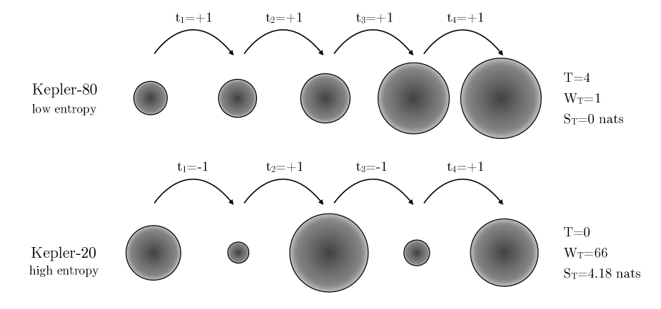
Figure 1: Example of the different planetary entropies for a five planet system. The circles depict the size ordering of planetary radii, in order of orbital separation from the star. The Kepler-80 planets appear sorted in terms of their radii, giving a tally of $T=4$, which can only be achieved in this single configuration, thereby yielding a low entropy. Vice versa, the Kepler-20 system is more disordered and high entropy. Size orderings are based on the maximum likelihood planet-to-star relative radii reported on the NASA Exoplanet Archive (Akeson et al., 2013).

2.2 The Number of Unique Microstates

As an initial definition for size-ordering entropy, we consider the changes between neighboring planets only. We may compute a size-ordering tally, $T$, for each system by going through each pair and assigning $t_{i}=+1$ if the outer planet is larger than the inner, and $t_{i}=-1$ otherwise. This simple algorithm is equivalent to the expression

$$t_{i} =2\mathbb{H}[R_{i+1}-R_{i}]-1,$$ (1)

which yields a total tally score of

$$T \equiv\sum_{i=1}^{N-1}t_{i},$$ (2)

where $R_{i}$ is the radius of the $i^{\mathrm{th}}$ planet and $N$ denotes the total number of planets in the system. One may show that the resulting entropy term we later compute using this definition is equivalent to different scoring schemes, such as replacing $t_{i}=-1$ with $t_{i}=0$.

Each score can be considered to be a micro-state, and in total there will be $N!$ possible microstates/scores and $\Omega_{T}$ unique micro-states/scores, where

$$\Omega_{T} =N.$$ (3)

To distinguish between unique microstates, we label each with the index $M$, such that $M=1,2,...,N-1,N$.

2.3 Determining Microstate Index

Whilst we have defined the number of unique microstates for $N$ planets, $\Omega_{T}$, the actual score ($T$) of each microstate is yet to be defined. One may show that the tally score of each unique microstates, $T$, will follow an arithmetic series, given by

$$T =-(N-1)+2(M-1).$$ (4)

Using the above, one can re-arrange to solve for $M$, the unique microstate index, for a given solution for $T$ and a choice of $N$, to yield

$$M =\frac{N+T+1}{2}.$$ (5)

Equation (5) essentially allows one to orient ourselves and convert an observed tally score into a location, in terms of unique microstate index.

2.4 Occupancies

Let us define the occupancy of each unique microstate as $W_{T}$. The minimum occupancy of a unique microstate (or the minimum frequency of a unique score) is always 1. For $N>1$, there are always exactly two unique microstates with an occupancy of $W_{T}=1$, which occur for $T_{\mathrm{max}}=(N-1)$ and $T_{\mathrm{min}}=-(N-1)$.

Consider ranking all of the unique microstates from smallest to largest $T$ and then labeling these ranks $M=1,2,...,N-1,N$ consecutively. The occupancy, $W_{T}$, of the $M^{\mathrm{th}}$ unique microstates is described by

$$W_{T} =A_{N,M-1},$$ (6)

where $A_{p,q}$ is the Eulerian number generating function given by

$$A_{p,q} \equiv\sum_{j=0}^{q}(-1)^{j}\binom{p+1}{j}(q-j+1)^{p}.$$ (7)

If $N$ is odd, then there will be just one unique microstate maximally occupied with $T=0$. Else, if $N$ is even, there will a pair of unique microstates/scores with maximal occupancy, given by $T=\{-1,+1\}$.

Combining our earlier result for $M$ as a function of $T$ (Equation 5), with Equation (6) above, allows us to directly evaluate $W_{T}$ from the score, $T$, using

$$W_{T} =A_{N,\tfrac{N+T-1}{2}}.$$ (8)

The scores and occupancies of each unique microstate, $T$ and $W_{T}$, are illustrated in Figure 2 up to $N=10$ (although one can extend our approach to arbitrarily large $N$).

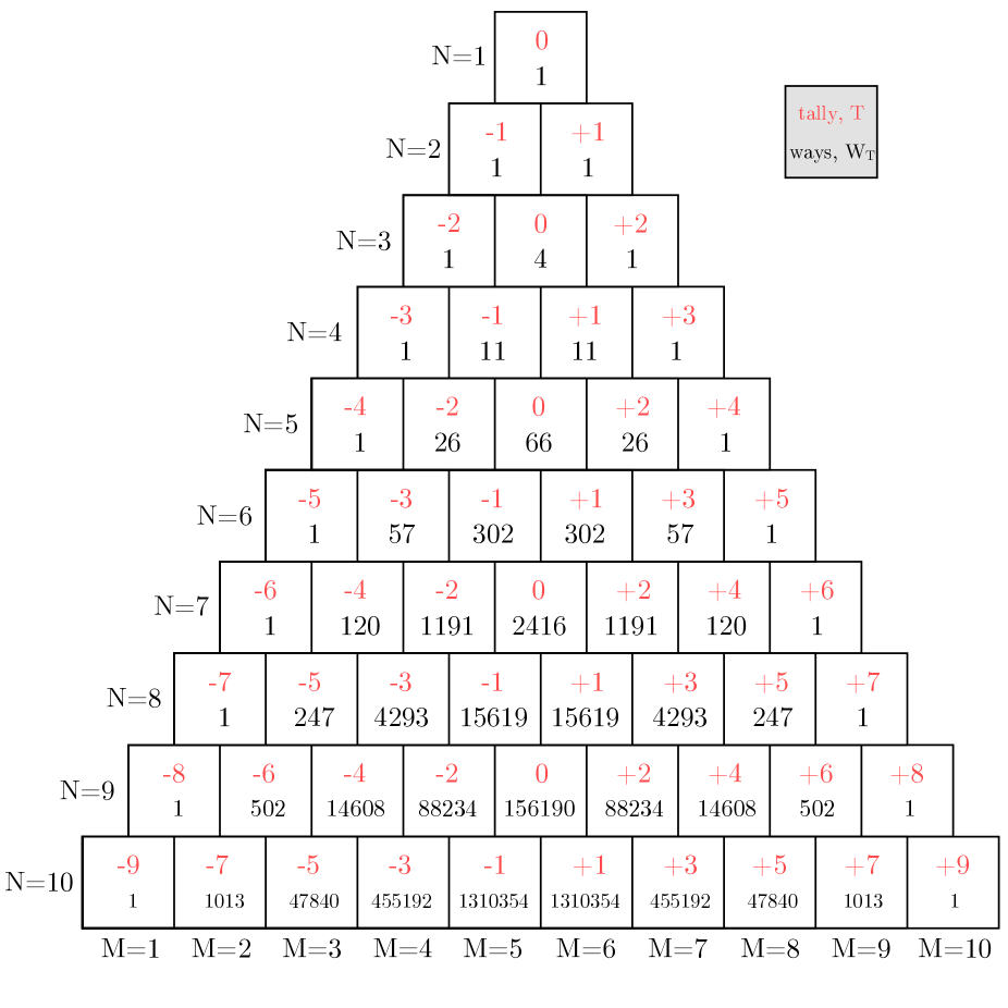
Figure 2: Illustration of the number of unique microstates for each choice of $N$. Each unique microstate is represented by a black box, with the red numbers giving the score, $T$, associated with that unique microstate and the black numbers giving the number of microstates which can produce this score, $W_{T}$.

The occupancy of each unique microstate can be considered to be the number of equivalent ways of obtaining the same score. In this way, we may define the entropy of each unique microstate as

$$S_{T}=\log W_{T},$$ (9)

where we use log base $e$ in what follows to give an entropy in units of nats.

The minimum entropy obtainable thus occurs for the maximum/minimum score, which has an occupancy of just one and thus $S_{T,\mathrm{min}}=\log 1=0$. The maximum entropy obtainable occurs for the most occupied microstate, which has an occupancy of $W_{T,\mathrm{max}}=A_{N,\lfloor N/2\rfloor}$ and thus $S_{T,\mathrm{max}}=\log A_{N,\lfloor N/2\rfloor}$. There are only $\lceil N/2\rceil$ unique possible entropies, which is less than or equal to the number of unique microstates, $N$ (since the $N^{\mathrm{th}}$ entropy vector is symmetric about the median element).

2.5 Evolving Entropy

A basic expectation of any definition of entropy is that it should increase over time. To investigate this, we generated a initially pristine system of $S_{T}=0$ such that the size orderings can be described by a vector containing an integer sequence. Given that our entropy is framed in terms of size-ordering, a suitable proxy for time would to allow exchanges between planets, for which local neighboring pairs would be the simplest method. To accomplish this, we chose a random element of the radii vector, followed by a random neighbor either preceding or proceeding the element. For end-members, there is only one choice for this element choice. The two elements are then exchanged, giving rise to a higher entropy system. We repeated this $10^{6}$ times with an exchange probability of $0.1$, leading to a final state which has been extremely well-mixed.

Although our algorithm only allows neighbors to swap, real physical systems may be able to exchange non-neighboring planets too. However, such exchanges can always be described by multiple neighboring swaps. We stress that the goal of this exercise is not to find a causal relation between iteration number and time, merely to qualitatively simulate the passage of time by allowing exchanges to occur at some finite rate.

As shown in Figure 3, the average entropy of the system indeed evolves ever-upwards, as expected for a entropy-like term. This establishes that specific examples of low-entropy systems, such as Kepler-80 (MacDonald et al., 2016), are highly unlikely to be the product of a purely random process. If their size-ordering configuration are not random, then this implies that they retain some information about a specific mechanism leading to their origin. In other words, such low-entropy systems are information-rich.

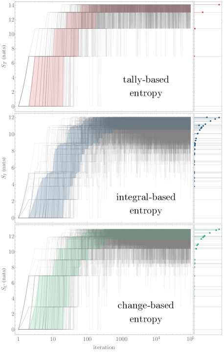
Figure 3: Evolution of the entropy of an initially pristine $N=10$ system where each iteration allows for a 10% probability swap of a random, neighboring planet-pair. The 100 faint gray lines show individual simulations, whereas the shaded region shows the 68.3% central quantile. The histogram on the right-hand side is that after $10^{6}$ iterations.

3 ENTROPY USING THE INTEGRAL PATH

3.1 The Solar System Counter Example

Although our definition of entropy appears to be characterizing disorder, the Solar System provides a counter example as to why our current definition is somewhat limited. For the $N=8$ planet Solar System, we find a score of $T=-1$, which has $W_{T}=15619$ ways of achieving (see Figure 4). Indeed, even replacing Mars with a Super-Earth, to create an apparently highly-ordered size ordering leads to the same entropy. Thus, the Solar System appears to be in the most highly disordered state possible. The clear size ordering trend present (Figure 4) elucidates that our definition is somehow inadequate and we consider why here.

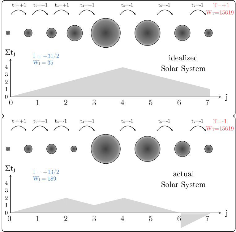
Figure 4: Illustration of the size ordering of the Solar System (not to scale) for the actual configuration and an “idealized” configuration replacing Mars with a Super-Earth. A tally-based entropy fails to detect the low entropy nature of even the idealized state, motivating us to define an improved definition using the integral-paths and change points, as depicted.

First, consider that the Solar System planets increase in size from the inner most planet, Mercury, up to Jupiter (with the exception of Mars), leading to a high tally by the time we reach Jupiter. After this point, the planets regularly decrease in size down to Neptune. Consequently, the high positive score attained up to Jupiter is cancelled out by the high negative score of the outer Solar System. Accordingly, this configuration scores the same as randomly mixing the planets up.

This point illustrates what is wrong with our current definition for the score - it does not have a memory. A score which flips randomly from one planet to the next should be more disordered than a regular increase followed by a regular decrease. We thus need to adapt our entropy definition to include a term accounting for the autocorrelation or memory of the previous scores.

We devised two modifications to our simple tally system, one based on the integral path and the other based on change points. We discuss the latter later in Section 4, and consider the integral path modification in what follows.

3.2 Number of Unique Sub-Microstates

Instead of considering each microstate as solely defined by the tally, $T$, we consider that it is defined by a vector containing two numbers, $T$ and another term chosen to incorporate a memory-like property. This much like how a thermodynamic microstate can be defined by two degrees of freedom, rather than just one for example. One way to think about this is that we have split the original $M^{\mathrm{th}}$ microstate into $\omega_{I,M}$ “sub-microstates”, denoted by the labels $k=1,2,...,\omega_{I,M}-1,\omega_{I,M}$. The term “sub-microstates” is formally incorrect, but it useful since it allows us to refer to these microstates relative to the original microstates derived using the tally-based system. For this reason, we will use the term in what follows but stress it is only for linguistic convenience.

A possible choice for a second degree of freedom is the integral of $t_{i}$ over $i$. For example, $N$ consecutive increases in $t_{i}$ can be thought of a line enclosing a triangular area below the curve (a linear interpolation). Let us define this integral as $I$, which we use as the second term in a vector, such that each unique sub-microstate is now defined by $\{T,I\}$.

We find that this definition is effective at splitting up the originally defined microstates into a finer grid of sub-microstates and also brings the Solar System down into a much lower entropy state, as desired (as shown later).

We find that the number of unique microstates grows from $\Omega_{T}=N$ to $\Omega_{I}=\mathcal{C}_{N-1}$ sub-microstates, where $\mathcal{C}_{k}$ is a Cake number, the maximum number of regions which a three-dimensional cube can be partitioned by exactly $N$ planes, defined by

$$\mathcal{C}_{k} =\sum_{i=0}^{k}\binom{k}{i}=\frac{k^{3}+5k+6}{6}.$$ (10)

On a finer scale, the $M^{\mathrm{th}}$ microstate is expanded into $\omega_{I,M}=[(N-M)(M-1)+1]$ sub-microstates. This was identified by noting that the sequence follows the rascal triangular number sequence. When summed over $M=1$ to $M=N$, this yields the expected result of $\Omega_{I}=\sum_{M=1}^{N}\omega_{I,M}=\mathcal{C}_{N-1}$ total number of sub-microstates. In Figure 5, we show an example of how an array of microstates is split into $\Omega_{I}$ sub-microstates in the case of $N=6$.

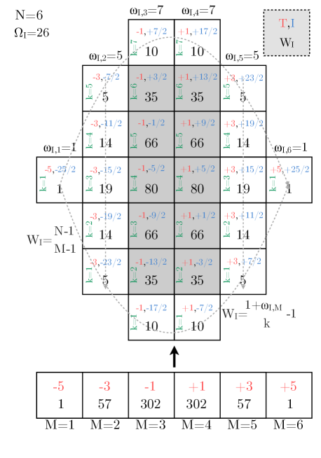
Figure 5: Schematic example of how a list of microstates based on tally-scoring (bottom row) is split into sub-microstates using the integral-path based entropy system. The dashed lines depict sub-microstates where we are able to find analytic formulae to predict the occupancies, and the shaded sub-microstates are those for which no analytic solution was found and thus we rely on pre-computed libraries.

3.3 Determining Sub-Microstate Index

Before we deal with the occupancies of each sub-microstate, we first require a means to convert an observed pair of scores, $\{T,I\}$, into a sub-microstate index, given by the numbers $M$ and $k$. The index $M$ is still determined using the same procedure as before, i.e. it is given soley by the tally $T$ and Equation (5). To complete the picture then, we need a means to convert an observed integral score, $I$, into an index $k$.

To do this, we follow a similar procedure to that used in Section 2.3 and first write down the forward-case of the integral as function of $k$, which we find can be written as

$$I(k)=\begin{cases}2k-I_{\mathrm{max}}&\text{if }M\leq\tfrac{N}{2},\\ I_{\mathrm{max}}-2k&\text{if }M>\tfrac{N}{2}.\\ \end{cases},$$ (11)

where $I_{\mathrm{max}}$ is the maximum $I$ score for each index $M$, given by

$$I_{\mathrm{max}} =\tfrac{1}{2}(N-1)^{2}-(\mathrm{Min}[M-1,N-M])^{2}.$$ (12)

In practice, we convert an $I$-score into $k$ by writing out the full list of possible $I$-scores for each $k$ with Equation (11) and then selecting the matching example.

3.4 Occupancies

The occupancy of these sub-microstates, which we denote using the symbol $W_{I}$, does immediately appear to follow a well-known number sequence, but we do observe that the extreme values of $W_{I}(M,k=1)$ follows Pascal’s triangular number sequence along the axis $M=1$ to $M=N$. The same is true for the opposite extreme of $W_{I}(M,k=\omega_{I,M})$, such that

$$W_{I}(M,k=1||\omega_{I,M}) =\binom{N-1}{M-1}=\frac{(N-1)!}{(M-1)!(N-M)!}.$$ (13)

We also know the sum of the occupancies across all sub-microstates for a fixed choice of $M$ must equal the $M^{\mathrm{th}}$ microstate’s occupancy, such that

$$\sum_{k=1}^{\omega_{M,I}}W_{I}(M,k) =A_{N,M-1}$$

$$=\sum_{j=0}^{M}(-1)^{j}\binom{N+1}{j}(M-j)^{N},$$ (14)

where the above illustrates the two sums above cannot be directly equated since they use different summation indices.

Thirdly, we note that the second columns, $M=2$ and $M=(N-1)$ appear to follow a well-known sequence, specifically the Pascal’s triangle -1, such that

$$W_{I}(M=2,k)= \binom{1+\omega_{I,M}}{k}-1\,\,\forall\,\,k\in\{1,2,...,\omega_{I,M}\},$$ (15)

where we write the formula in two equivalent ways and note that $W_{I}(M=2,k)=W_{I}(M=\omega_{I,M}-1,k)$.

Aside from these specific cases, we are unable to find a general analytic form for the $W_{I}(M,k)$ and thus $W_{I}(T,I)$, Instead, we numerically computed all possible permutations of 1 to 10 planet systems, counted the occupancies of each sub-microstate and then saved them to a library function. In instances where the aforementioned specific cases hold, we employ the analytic solution instead. This Python code is made available at this URL.

3.5 Properties

As noted, including integral path as a second degree of freedom lowers the entropy of the Solar System. Further, as with the tally-based entropy, we verified that random swapping leads to ensemble increasing in entropy over time, as depicted in Figure 3. As can also be seen from this figure and using the equations above, that the total number of unique microstates is higher with this definition, leading to a finer array of possible entropies and thus a lower maximum entropy in an absolute sense.

4 ENTROPY USING CHANGE POINTS

4.1 Number of Unique Sub-Microstates

In addition to integral paths, we devised a alternative way to define the second degree of freedom based on the number of “change points” which occur in the tally history. This essentially serves like a derivative tally-layer, where we append $+1$ if $t_{i+1}$ is different from $t_{i}$, or $+0$ otherwise. We may write the change point tally, $C$, as

$$C =\sum_{i=1}^{N-2}(1-\delta[t_{i},t_{i+1}])$$ (16)

where $\delta[p,q]$ is the Kronecker Delta function and now each unique sub-microstate is now uniquely defined by $\{T,C\}$. To distinguish from before, we label the occupancy of each sub-microstate with the notation $W_{C}$.

As before, we find that this definition is effective at splitting up the originally defined microstates into a finer grid of sub-microstates and again brings the Solar System down into a lower entropy state, from $W_{T}=15619$ to $W_{C}=3472$. When replacing Mars with a Super-Earth to create an “idealized” Solar System, the difference is greater, going from $W_{T}=15619$ to $W_{C}=70$ (see Figure 4).

When using change points, the $M^{\mathrm{th}}$ microstate is divided into $\omega_{C,M}$ sub-microstates, where

$$\omega_{C,M} =2\mathrm{Max}\big{[}\mathrm{Min}[M-1,N-M],\tfrac{1}{2}\big{]}-\delta_{\tfrac{N-1}{2},M-1}.$$ (17)

Summing over all $N$ and simplifying, we find that the number of unique microstates grows from $\Omega_{T}=N$ to

$$\Omega_{C} =\lfloor((N-1)^{2}+3)/2\rfloor.$$ (18)

In Figure 6, we again show an example of how an array of the tally-based microstates is split into $\Omega_{C}$ sub-microstates using the change point system.

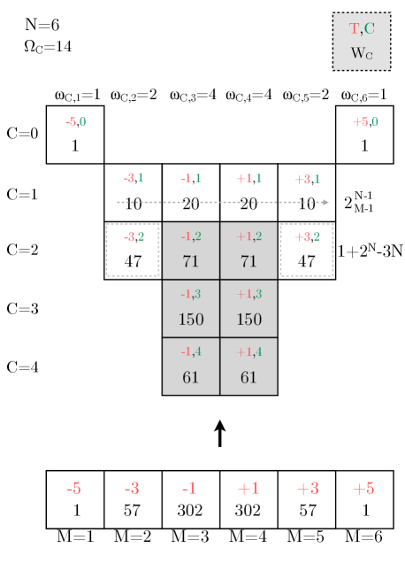
Figure 6: Schematic example of how a list of microstates based on tally-scoring (bottom row) is split into sub-microstates using the change point based entropy system. The dashed lines/boxes depict sub-microstates where we are able to find analytic formulae to predict the occupancies, and the shaded sub-microstates are those for which no analytic solution was found and thus we rely on pre-computed libraries.

4.2 Determining Sub-Microstate Index

We briefly point out that unlike the integral-scoring system, the sub-microstate index for change points is defined by the change point score itself without manipulation (e.g. see Figure 6). For this reason, there is no issue with having to perform a conversion here.

4.3 Occupancies

The occupancies of these sub-microstates, $W_{C}$, does not immediately appear to follow a well-known number sequence, but we do observe that the extreme values of $\lim_{C\to 0}W_{I}=1$, where incidentally $C=0$ can only occur for $M=1$ or $M=N$.

We also find that the $C=1$ row follows a binomial-like pattern, specifically

$$\lim_{C\to 1}W_{C} =2\binom{N-1}{M-1},$$ (19)

where we note that $C=1$ occurs for all $M$ where $M\neq 1$ or $M\neq N$.

We also know the sum of the occupancies across all sub-microstates for a fixed choice of $M$ must equal the $M^{\mathrm{th}}$ microstate’s occupancy, such that

$$\sum_{C=0}^{\omega_{C}}W_{C}(M,N,C) =A_{N,M-1}$$

$$=\sum_{j=0}^{M}(-1)^{j}\binom{N+1}{j}(M-j)^{N}.$$ (20)

Note that, in general, $\omega_{C,M}\neq M$, such that the summation indices are distinct in the above and thus this does not provide a candidate general formula for $W_{C}$.

Finally, for $M=2$ or $M=N-1$, Equation (17) implies that $\omega_{C,M}(C=2)=\omega_{C,M}(C=N-1)=2$ for all $N$. Therefore, since we know $W_{C}(C=1)$ (Equation 19), and we know the sum of the occupancies across all sub-microstates for any $M$, then we can write

$$W_{C}(T,C=2)= \Bigg{[}\sum_{j=0}^{M}(-1)^{j}\binom{N+1}{j}(M-j)^{N}\Bigg{]}$$

$$-\lim_{M\to 2||N-1}\Bigg{[}2\binom{N-1}{M-1}\Bigg{]},$$

$$=1+2^{N}-3N.$$ (21)

Beyond this result, we are unable to find any other analytic formula to expedite the calculation of occupancies. Instead, and as before, we ran numerical experiments exploring all permutations of planetary size orderings for each $N$ up to $N=10$ and then simply counted the occupancies. These results were coded up into a Python library (see this URL), such that for any given $T$ and $C$ combination, one can simply look-up the corresponding $W_{C}$, leveraging the analytic results from above wherever possible.

4.4 Properties

As with the integral path, including change points as a second degree of freedom decreases the entropy of the Solar System. Further, as with both previous systems, we again find that random swapping leads to ensemble increasing in entropy over time, as expected and depicted in Figure 3. As with the other definitions then, the observation of a low entropy state can be stated to be unlikely to arise from random swaps over time and the observation of an ensemble of systems with low entropy is highly unlikely to arise from random swaps. In other words, such low entropy states are fundamentally not random but contain some information about a guiding process leading preferentially to such low entropy configurations.

5 APPLYING TO KEPLER SYSTEMS

5.1 Interpreting Entropy

In this section, we apply our entropy scoring system to real planetary systems. Before doing so, we briefly highlight some conclusions which can be made using an entropy score.

For an individual system found to have a low entropy (using any of previously discussed metrics), the $p$-value of observing such an entropy under the hypothesis that all systems are randomly organized can be computed. By “randomly organized”, we specifically refer to the simulations introduced in Section 2.5 i.e. initially zero-entropy systems allowed to undergo a large number of position exchanges. The $p$-value computation is performed by simply evaluating the median rank of the observed entropy within the sorted list of Monte Carlo simulated final states for random systems.

To give an example of the above, consider the $N=5$ planet system Kepler-80 (MacDonald et al., 2016), which was depicted earlier in Figure 1. Kepler-80 exists in a perfectly ordered configuration, giving $S_{T}=S_{I}=S_{C}=0$. Even from a sample of $10^{6}$ randomly generated systems, we find 0 instances of such a low entropy for any of metric and thus infer that $p_{T},p_{I},p_{C}\leq 10^{-6}$.

The $p$-values quoted, a measure of surprisingness, reveal that even amongst a sample of several thousand planetary systems, such a low entropy score is not expected. We attribute this as evidence that Kepler-80 contains a memory of a specific formation pathway which presumably is described by some unknown entropy distribution with a greater probability density at low entropy values. In plainer terms, Kepler-80 appears to remember something of its origin.

Ideally, this process could be repeated on all of the Kepler systems. However, the argument above has ignored measurement uncertainties and this introduces a major obstacle to realizing an entropy for each system. In many cases, the measurement uncertainties reported on the NASA Exoplanet Archive (NEA; Akeson et al. 2013) are sufficiently wide that one should expected a significant fraction of the joint posterior samples to lead to distinct entropy scores. Essentially, this implies we need to derive a posterior for the entropy.

Marginal posterior distributions of each planet’s ratio-of-radii could be used to achieve this. However, we are aware of no such public catalog at this time that treats planets with the same parent star as transiting a star with a global set host star parameters and covariant individual planet parameters (Sandford & Kipping 2017 present such posteriors but only for a subset of Kepler stars). Instead, we generate representative posteriors using the method described in what follows.

5.2 Generating Asymmetric Posteriors

We first downloaded the list of reported ratio-of-radiis from NEA (Akeson et al., 2013) for every Kepler system with $N\geq 3$ planets, for which the host star satisfied $\log g>4$ and has an exoplanet disposition of being either candidate or confirmed (224 systems). Typically, the ratio-of-radii are reported with asymmetric measurement uncertainties, meaning that one cannot simply treat them as being described by a normal distribution, which is symmetric.

To create an asymmetric distribution, we used a mixture of two truncated normals, where the first normal is truncated from $0$ up to the reported mean, and the second is truncated from the reported mean up to unity. To ensure a smooth probability distribution at the boundary, the mixture weights are set to the ratio of each density at the mean’s location, leading to a normalized and smooth asymmetric distribution. Specifically, for a measurement of $p=\mu_{-\sigma_{-}}^{+\sigma_{+}}$, our model treats $p$ as being distributed as

$$p\sim\begin{cases}\mathcal{T}[\{0,\mu\},\mathcal{N}[\mu,\sigma_{-}]]&\text{if }p\leq\mu,\\ \mathcal{T}[\{\mu,1\},\mathcal{N}[\mu,\sigma_{+}]]&\text{if }p>\mu,\\ 0&\text{otherwise},\end{cases}$$ (22)

where $\mathcal{N}[a,b]$ is a normal distribution and $\mathcal{T}[\{\alpha,\beta\},\mathcal{X}]$ is a truncated distribution of $\mathcal{X}$. The resulting probability density function is plotted in Figure 7 for some example inputs.

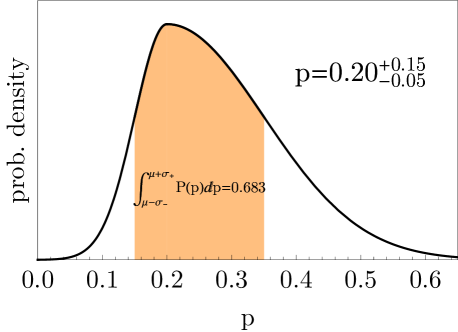
Figure 7: Example of an asymmetric probability distribution generated using our weighted mixture model of truncated normals.

We performed inverse transform sampling of the distribution to generate $10^{4}$ fair realizations of each planet’s ratio-of-radii. We then repeat our calculation of the size-ordering entropy on each realization to build an entropy posterior for each system. In the case of Kepler-80, we find that the entropies are measured to be $S_{T}=0_{-0}^{+4.2}$ nats, $S_{I}=0_{-0}^{+2.8}$ nats and $S_{C}=0_{-0}^{+3.1}$ nats, which illustrates the considerable effect of current measurement uncertainties.

Critically, our model does not account for covariance which would lead to tighter constraints on the resulting entropy posteriors. Ultimately, our model is therefore accurate but less precise than possible and future work could revisit the calculations described below when covariant posteriors become available.

5.3 Application to Kepler Multis

We applied our algorithm to the 224 Kepler multi-planet systems described earlier. Grouping the systems into their unique $N$ values, we find 151 three-planet systems, 50 four-planet systems, 19 five-planet systems and 4 six-planet systems. For each system, we computed all three entropy scores and then created histograms of the resulting distributions of the best-reported ratio-of-radii, shown in Figure 8.

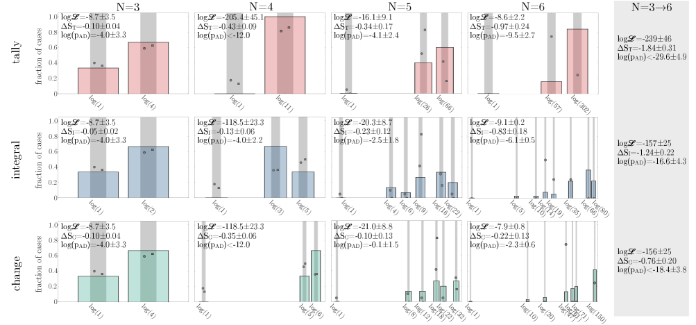
Figure 8: Summary of results comparing the entropy of multiple planet Kepler systems (columns) for three different entropy-scoring methods (rows). Final column adds up the multis together, reflecting the consistent pattern of Kepler multis (circles with Poisson counting error bars) having a lower entropy than random systems (bar histograms). Squares points are the same Kepler systems but filtering on only those thought to be dynamically packed.

Each panel in Figure 8 is for $N=3,4,5,6$ across and $S_{T},S_{I},S_{C}$ down. In the top-left of each panel, we report three summary statistics of interest, where the best-reported value is that derived using the best-reported ratio-of-radii, whereas the “$\pm$” uncertainty is the standard deviation of each metric across $10^{4}$ random posterior draws of the ratio-of-radii, as described earlier.

The three metrics considered are $\log\mathcal{L}$ assuming a binomial distribution at each unique microstate, the mean entropy of the population minus that of a random population, $\Delta S$, and the $p$-value derived from comparing the observed population with a random population using the Anderson-Darling test, $\log(p_{\mathrm{AD}})$.

Across the board, we consistently find that the Kepler population has a lower entropy than the random population for all $N$ and entropy scoring systems, although the magnitude and significance varies considerably. Combining the metrics for all planet groupings on the far-right column of Figure 8 shows that there is very strong evidence for an entropy deficit amongst the Kepler systems, ranging from at best 22 $\sigma$, using the tally-based binomial likelihood, to at worst $3.8$ $\sigma$, using the mean entropy of the change-point entropy. The Anderson-Darling tests typically sit between two extremes, suggesting a $\sim 6$ $\sigma$ effect.

Considering each $N$ grouping separately, we note that $N=4$ group seems to show a particularly pronounced entropy deficit, so extreme that we were unable to compute numerically stable Anderson-Darling $p$-values. In general, the trend appears to be that $N=3$ systems show a modestly significant deficit, it becomes extreme for $N=4$ and then drops down with increasing $N$. This downward trend is likely due to the ever-smaller samples sizes with increasing $N$ which naturally attenuate significances. The $N=3$ case may be explained by the fact that only two unique microstates are possible for all three entropy-scoring systems and random systems tend to populate both with non-negligible fractions.

Since the integral path system does the best job of explaining the Solar System, we tend to prefer it in this work. Accordingly, we conclude that there is $(5.4\pm 0.8)$ $\sigma$ evidence for an entropy deficit in the ensemble of Kepler multis using the Anderson-Darling test, and a consistent $5.6$ $\sigma$ confidence when using the means testing. This analysis indicates that the ensemble of Kepler multi-planet systems exist in a lower entropy state than that of pure randomization. In other words, the Kepler systems contain some information or memory of their (non-random) origin mechanism, since they are highly unlikely to have arrived in their observed configuration as a result of random exchanges. In many ways the above statement may sound completely expected, yet we have shown here that the statement is non-trivial to formally prove.

5.4 Dynamically Packed Systems

Our definition of entropy is sensitive to missing planets. An obvious set of missing planets are those beyond 1 AU, where transit surveys like Kepler have weak sensitivity (Beatty & Gaudi, 2008; Kipping & Sandford, 2016b). However, the entropies measured interior to 1 AU are still valid when treated as the local entropy score of this region. A much more problematic situation is the case of one or more missing planets interior to the outer-most detected planet but exterior to inner-most detected planet. These worlds will cause even this local entropy score to be erroneous and thus we consider how to mitigate against this effect here.

However, we first highlight that the Kepler multi-planet systems have been demonstrated to exhibit low mutual inclinations (consistent with $\lesssim 3^{\circ}$; Lissauer et al. 2011; Tremaine & Dong 2012; Fang & Margot 2012; Fabrycky et al. 2014; Ballard & Johnson 2016), which makes it geometrically improbable for a planet interior to the outermost transiting planet to be missing i.e. non-transiting. Much more likely is that the planet is missing due to detection effects, most plausibly because the planet is so small it evaded detection.

To investigate this, we may use the generalized Titius-Bode law (Bovaird & Lineweaver, 2013) as a proxy for dynamical packing, for the following reasons. Consider a $N$-planet system which is dynamically packed, such that the planets are so close together that additional planets cannot be injected into intermediate orbits. Such a configuration implies that the planets are separated by just $k$ Hill radii, where $k$ is some number greater than one controlling the spacing and the Hill radius of the $i^{\mathrm{th}}$ planet, $H_{i}$, is given by

$$H_{i} =a_{i}\Big{(}\frac{\mathcal{M}_{i}}{3}\Big{)}^{1/3},$$ (23)

where $\mathcal{M}_{i}$ represents the mass ratio between the $i^{\mathrm{th}}$ planet and the star.

For $N=2$ planet systems, $k=2$-$4$ is expected to ensure stability (Wetherill & Cox, 1984, 1985; Lissauer, 1987; Wetherill, 1988; Gladman, 1993) but for $N>2$, no choice of $k$ is indefinately stable, rather the stability time increases with $k$ such that $k\gtrsim 13$ provides Gyr stability to a Solar System analog (Chambers et al., 1996). For our purposes, it is unimportant what value $k$ actually is, but let’s proceed to treat it is a fixed number. Accordingly, semi-major axes of the $i^{\mathrm{th}}$ and $(i+1)^{\mathrm{th}}$ planet, $a_{i}$ and $a_{i+1}$, must satisfy

$$a_{i+1}+kH_{i+1} \geq a_{i}-kH_{i},$$ (24)

which in the limit of the equality gives

$$a_{i+1} =a_{i}\frac{1+3^{-1/3}k\mathcal{M}_{i}^{1/3}}{1-3^{-1/3}k\mathcal{M}_{i+1}^{1/3}}.$$ (25)

Converting from semi-major axes to periods via Kepler’s Third Law (and assuming $\mathcal{M}_{j}\ll 1$) gives

$$P_{i+1} =P_{i}\Bigg{(}\frac{1+3^{-1/3}k\mathcal{M}_{i}^{1/3}}{1-3^{-1/3}k\mathcal{M}_{i+1}^{1/3}}\Bigg{)}^{3/2},$$ (26)

or

$$\log(P_{i+1}) =\log(P_{i})+\underbrace{\tfrac{3}{2}\log\Bigg{(}\frac{1+3^{-1/3}k\mathcal{M}_{i}^{1/3}}{1-3^{-1/3}k\mathcal{M}_{i+1}^{1/3}}\Bigg{)}}_{=\log\alpha}.$$ (27)

This result essentially states that in the limit of low mass ratios, planets separated by $k$ Hill radii will follow the generalized Titius-Bode (GTB) law of Bovaird & Lineweaver (2013), i.e. that

$$\log P_{i} =P_{1}+(i-1)\log\alpha.$$ (28)

This result is consistent with that found by Hayes & Tremaine (1998), who use numerical integrations to demonstrate that the GTB law is simply a consequence of dynamical stability of packed systems.

We may now use the GTB law as a simple proxy to detect dynamically packed systems, without conducting detailed N-body tests such as those presented in Fang & Margot (2013). To accomplish this, we compare how well $\log\alpha$ agrees between consecutive pairs of planets in a system. If $\log\alpha$ is consistent amongst all pairs, then it can be said that the GTB law holds and the planets are consistent with being dynamically packed.

This criterion requires some quantification since small deviations in $\log\alpha$ are to be expected by varying the mass ratios, $\mathcal{M}_{i}$, and $k$, as can be seen from Equation (27). Accordingly, we evaluated the range of $\log\alpha$ values expected as a function of $k$ for mass-ratio ranges from 0.1 - 10 $M_{\oplus}$, consistent with the typical Kepler planets. We find that the fractional variation in $\log\alpha$ rises from $\simeq\tfrac{1}{4}$ for $k=1$ to $\simeq\tfrac{1}{3}$ for $k=20$. We therefore elect to use a third as a tolerance level to test for.

Applying this criterion reduces the samples sizes slightly. Specifically, we find go from 151 to 103 three-planet systems, 50 to 30 four-planet systems, 19 to 6 five-planet systems and 4 to 0 six-planet systems.

After filtering, we repeated the analysis described in Section 5.3 for each $N$, and the points are plotted in Figure 8 as squares (except for $N=6$ where no packed systems were identified). The results and metrics are broadly consistent with slightly deflated significances due to the smaller sample size under investigation. We find that the total entropy differences between the Kepler $N=3\to 5$ planet systems and a randomly generated population are $\Delta S_{T}=-0.77\pm 0.38$, $\Delta S_{I}=-0.22\pm 0.27$ and $\Delta S_{C}=-0.26\pm 0.30$. The Anderson-Darling test again supports strong evidence for a distinct population, with $p$-values of 5.8, 5.1 and 4.7 $\sigma$ for the tally-, change- and integral-based entropies.

5.5 Comparison to other approaches

The entropy methods devised and applied in this work are tailored to our specific problem in mind, yet we highlight that there is a large prior literature for checking randomness. A classic example is the Wald-Wolfowitz runs test, which is a non-parametric tool for evaluating the randomness of a binary sequence, allowing one to test the hypothesis that the elements of a sequence are mutually independent (Bradley, 1968). The sequence of planetary radii within a system is, of course, not a binary sequence but rather represented by a set of continuous, real numbers. However, we may apply the runs test to the tally-scores, which asks whether the next member is larger or smaller than the previous.

The runs test, therefore, can be a useful tool in the context of the evaluating the surprisingness of the tally-based entropy method’s resulting tally sequence. However, it does not delineate the results into distinct classes nor quantify the information content, in the same way an entropy scheme can (although we highlight that contemporary work has tried to connect the classic runs test to entropy scores; e.g. Rukhin 2000; Kraskov et al. 2004; Gan & Learmonth 2015). Going further, the test was obviously not designed with the planet problem in mind, and does not capture our physical insights that the lowest-entropy systems should be described by just two sequences, as our integral-based aims to account for.

Another common approach we highlight is the binary entropy function, $H_{b}$, which returns the entropy of a Bernoulli process of probability, $p$:

$$H_{b} =-p\log p-(1-p)\log(1-p),$$ (29)

where using natural log returns an entropy score in nats. For example, a fair coin with $p=0.5$ has the maximum possible entropy score of $H_{b}=1.44$ nats. At a basic level, this entropy score is fundamentally different from those considered in this work since we do not assume that the tally scores derived from a sequence of planetary radii follow a Bernoulli distribution. Rather, we simply compute the full range of possible configurations, assign entropies based on proxy scores and associated microstate occupancies, and then test for significance using Monte Carlo experiment. In the binomial entropy context, the entropy is used as a measure of uncertainty about a process or event, whereas our entropy scores are designed to be a measure of randomness.

We also highlight that there exists a suite of contemporary tests for quantifying the entropy of random number generators used in computer simulations, such as the Diehard tests, but these generally focus on very long sequences (unlike considered here) and, as before, were not designed to capture physical intuition for planetary systems.

6 DISCUSSION

We have presented three different formalisms for evaluating the entropy of planetary systems, in terms of their size orderings. Inspired by the stark contrasts between ostensibly ordered systems, like Kepler-80 (MacDonald et al., 2016), and disordered systems, like Kepler-20 (MacDonald et al., 2016), our work aims to provide a quantitative framework for evaluating these evident qualitative differences.

Using a tally-based scoring system, an integral-path method and a change-point system, we show that all three have marginal entropies that increase with respect to a proxy for time, as should be expected. We provide a detailed mathematical account of our definitions and show that much, but not all, of the microstate occupancies can be expressed with closed-form solutions, enabling fast computation. Cases without such solutions are folded in using look-up tables, culminating in our public Python package for evaluating the different entropies at this URL.

Through Monte Carlo simulation, we predict the expected distribution of the entropies for various $N$-planet systems after they have evolved from a large number of random swaps. When comparing this randomly-generated distribution to that of the real Kepler systems, we consistently find an entropy deficit in the real data to high confidence. Since the Kepler systems exhibit lower entropy than that expected of pure random swaps, the origin of their entropy values is highly unlikely to be random. In other words, they must contain some information or memory about the specific conditions which led to their original configuration, which may have been partially eroded by subsequent dynamical evolution. Nevertheless, the formal demonstration that the size-ordering of Kepler multis contains information establishes that efforts to infer initial formation conditions are not necessarily in vein.

We highlight that there is much room for improvement upon our proposed entropy schemes. First, planets of nearly equal sizes versus planets of vastly different sizes will yield the same entropy score for the same size ordering. We encourage future work to investigate the value of adding in a Boltzmann-like constant in front of our entropy definition, for which an obvious candidate is the variance of the sizes. Second, our definition does not address the specific distribution of orbital separation, merely their rank order. It may be possible to add such a term, although this is complicated by the dynamical preference for near mean-motion resonances of various orders.

Finally, we have not investigated the possibility of entropy differences between different sub-populations. Since entropy is expected to increase with respect to time, it should behave as an age-proxy, although it is unclear whether the time-scale for significant entropy evolution is comparable to the typical ages of observed systems. Regardless, it would be worthwhile to investigate if young versus old stars harbor different entropies. Similarly, one might expect binary stars to induce greater dynamical mixing and thus lead to high entropies. Such investigations are non-trivial since a complete and precise catalog of stellar ages and binarity do not presently exist for the Kepler sample, nor do mulit-planet covariant transit posteriors necessary for precise population comparison work. For these reasons, we highlight these as possible objectives for future work at this time.

As a concluding remark, we hope that this work encourages research into the relativity young discipline of “exo-informatics”, a field which can complement the broader population-based statistical inference approaches coming into play.

References

- Akeson et al. (2013) Akeson, R. L., Chen, X., Ciardi, D., et al. 2013, PASP, 125, 989
- Ballard & Johnson (2016) Ballard, S., & Johnson, J. A. 2016, ApJ, 816, 66
- Basri et al. (2005) Basri, G., Borucki, W. J., & Koch, D. 2005, New A Rev., 49, 478
- Batygin & Laughlin (2008) Batygin, K., & Laughlin, G. 2008, ApJ, 683, 1207
- Beatty & Gaudi (2008) Beatty, T. G., & Gaudi, B. S. 2008, ApJ, 686, 1302
- Bovaird & Lineweaver (2013) Bovaird, T., & Lineweaver, C. H. 2013, MNRAS, 435, 1126
- Bradley (1968) Bradley, J. 1968, Distribution-free statistical tests (Prentice-Hall)
- Buchhave et al. (2012) Buchhave, L. A., Latham, D. W., Johansen, A., et al. 2012, Nature, 486, 375
- Burke et al. (2015) Burke, C. J., Christiansen, J. L., Mullally, F., et al. 2015, ApJ, 809, 8
- Chambers et al. (1996) Chambers, J. E., Wetherill, G. W., & Boss, A. P. 1996, Icarus, 119, 261
- Ciardi et al. (2013) Ciardi, D. R., Fabrycky, D. C., Ford, E. B., et al. 2013, ApJ, 763, 41
- Dawson & Murray-Clay (2013) Dawson, R. I., & Murray-Clay, R. A. 2013, ApJ, 767, L24
- Deck et al. (2012) Deck, K. M., Holman, M. J., Agol, E., et al. 2012, ApJ, 755, L21
- Fabrycky et al. (2014) Fabrycky, D. C., Lissauer, J. J., Ragozzine, D., et al. 2014, ApJ, 790, 146
- Fang & Margot (2012) Fang, J., & Margot, J.-L. 2012, ApJ, 761, 92
- Fang & Margot (2013) —. 2013, ApJ, 767, 115
- Fischer & Valenti (2005) Fischer, D. A., & Valenti, J. 2005, ApJ, 622, 1102
- Fressin et al. (2012) Fressin, F., Torres, G., Rowe, J. F., et al. 2012, Nature, 482, 195
- Gan & Learmonth (2015) Gan, C. C., & Learmonth, G. 2015, ArXiv e-prints, arXiv:1512.00725
- Gladman (1993) Gladman, B. 1993, Icarus, 106, 247
- Gonzalez (1997) Gonzalez, G. 1997, MNRAS, 285, 403
- Han et al. (2014) Han, E., Wang, S. X., Wright, J. T., et al. 2014, PASP, 126, 827
- Hayes & Tremaine (1998) Hayes, W., & Tremaine, S. 1998, Icarus, 135, 549
- Johnson et al. (2010) Johnson, J. A., Aller, K. M., Howard, A. W., & Crepp, J. R. 2010, PASP, 122, 905
- Kipping (2013) Kipping, D. M. 2013, MNRAS, 434, L51
- Kipping & Sandford (2016a) Kipping, D. M., & Sandford, E. 2016a, MNRAS, 463, 1323
- Kipping & Sandford (2016b) —. 2016b, MNRAS, 463, 1323
- Kolmogorov (1958) Kolmogorov, A. N. 1958, Doklady of Russian Academy of Sciences, 119, 1559
- Kraskov et al. (2004) Kraskov, A., Stögbauer, H., & Grassberger, P. 2004, Phys. Rev. E, 69, 066138
- Lichtenberg & Lieberman (1983) Lichtenberg, A. J., & Lieberman, M. A. 1983, Regular and stochastic motion
- Lin & Papaloizou (1986) Lin, D. N. C., & Papaloizou, J. 1986, ApJ, 309, 846
- Lissauer (1987) Lissauer, J. J. 1987, Icarus, 69, 249
- Lissauer et al. (2011) Lissauer, J. J., Fabrycky, D. C., Ford, E. B., et al. 2011, Nature, 470, 53
- MacDonald et al. (2016) MacDonald, M. G., Ragozzine, D., Fabrycky, D. C., et al. 2016, AJ, 152, 105
- Rukhin (2000) Rukhin, A. L. 2000, Journal of Applied Probability, 37, 88–100
- Sandford & Kipping (2017) Sandford, E., & Kipping, D. M. 2017, MNRAS
- Seager & Mallén-Ornelas (2003) Seager, S., & Mallén-Ornelas, G. 2003, ApJ, 585, 1038
- Shabram et al. (2016) Shabram, M., Demory, B.-O., Cisewski, J., Ford, E. B., & Rogers, L. 2016, ApJ, 820, 93
- Shannon (1948) Shannon, C. E. 1948, Bell System Technical Journal, 27, 379
- Shannon & Weaver (1949) Shannon, C. E., & Weaver, W. 1949, The mathematical theory of communication
- Shen & Turner (2008) Shen, Y., & Turner, E. L. 2008, ApJ, 685, 553
- Sinai (1959) Sinai, Y. G. 1959, Doklady of Russian Academy of Sciences, 124, 768
- Sliski & Kipping (2014) Sliski, D. H., & Kipping, D. M. 2014, ApJ, 788, 148
- Tremaine (2015) Tremaine, S. 2015, ApJ, 807, 157
- Tremaine & Dong (2012) Tremaine, S., & Dong, S. 2012, AJ, 143, 94
- Tsiganis et al. (2005) Tsiganis, K., Gomes, R., Morbidelli, A., & Levison, H. F. 2005, Nature, 435, 459
- Van Eylen & Albrecht (2015) Van Eylen, V., & Albrecht, S. 2015, ApJ, 808, 126
- Walsh et al. (2011) Walsh, K. J., Morbidelli, A., Raymond, S. N., O’Brien, D. P., & Mandell, A. M. 2011, Nature, 475, 206
- Wang & Ford (2011) Wang, J., & Ford, E. B. 2011, MNRAS, 418, 1822
- Wetherill (1988) Wetherill, G. W. 1988, Accumulation of Mercury from planetesimals, ed. F. Vilas, C. R. Chapman, & M. S. Matthews, 670–691
- Wetherill & Cox (1984) Wetherill, G. W., & Cox, L. P. 1984, Icarus, 60, 40
- Wetherill & Cox (1985) —. 1985, Icarus, 63, 290