Deep Learning of Quasar Spectra to Discover and Characterize Damped Ly$\alpha$ Systems

Abstract

We have designed, developed, and applied a convolutional neural network (CNN) architecture using multi-task learning to search for and characterize strong HI Ly$\alpha$ absorption in quasar spectra. Without any explicit modeling of the quasar continuum nor application of the predicted line-profile for Ly$\alpha$ from quantum mechanics, our algorithm predicts the presence of strong HI absorption and estimates the corresponding redshift $z_{\rm abs}$ and HI column density $N_{\rm HI}$, with emphasis on damped Ly$\alpha$ systems (DLAs, absorbers with $N_{\rm HI}\geq 2\times 10^{20}\,{\rm cm^{-2}}$). We tuned the CNN model using a custom training set of DLAs injected into DLA-free quasar spectra from the Sloan Digital Sky Survey (SDSS), data release 5 (DR5). Testing on a held-back validation set demonstrates a high incidence of DLAs recovered by the algorithm (97.4% as DLAs and 99% as an HI absorber with $N_{\rm HI}>10^{19.5}\,{\rm cm^{-2}}$) and excellent estimates for $z_{\rm abs}$ and $N_{\rm HI}$. Similar results are obtained against a human-generated survey of the SDSS DR5 dataset. The algorithm yields a low incidence of false positives and negatives but is challenged by overlapping DLAs and/or very high $N_{\rm HI}$ systems. We have applied this CNN model to the quasar spectra of SDSS-DR7 and the Baryonic Oscillation Spectroscopic Survey (BOSS, data release 12) and provide catalogs of 4,913 and 50,969 DLAs respectively (including 1,659 and 9,230 high-confidence DLAs that were previously unpublished). This work validates the application of deep learning techniques to astronomical spectra for both classification and quantitative measurements.

1 Introduction

The dominant reservoirs of atomic hydrogen in the universe are traced by layers of HI gas referred to as the damped Ly$\alpha$ systems (DLAs). The DLAs are defined to have integrated HI column densities $N_{\rm HI}\geq 2\times 10^{20}\,{\rm cm^{-2}}$, sufficiently high to show damping wings driven by quantum mechanic broadening of the HI Ly$\alpha$ transition. These absorption lines are observed in the spectra of distance sources that emit at far ultraviolet wavelengths from gas both intrinsic to the source and intervening.

Wolfe et al. (1986) were the first to recognize that such absorption systems could be surveyed in the distant universe through spectroscopy of high $z$ quasars. Their primary motivation was to reveal conditions in the interstellar medium (ISM) of distant galaxies, expecting that very high $N_{\rm HI}$ absorption would trace gas primarily within galaxies. Using the 4m-class telescopes of that time, their initial and subsequent surveys derived a sample of $\sim 100$ DLAs at $z\sim 2$ (Lanzetta et al., 1995; Wolfe et al., 1995). The discovery and analysis of these DLAs were pursued primarily with visual inspection and by-eye fits to the Ly$\alpha$ absorption using Voigt profiles. These surveys established that DLAs are uncommon ($\approx 1$ system per 4 sightlines) and offered the first estimates of the cosmological mass density of neutral hydrogen.

Follow-up observations of metal-line transitions from heavy elements enriching the gas have enabled additional scientific exploration on the physical conditions within the interstellar medium of distant galaxies. This includes the chemical evolution of galaxies in the early Universe (Pettini et al., 1997; Prochaska and Wolfe, 2000), dust depletion, nucleosynthetic enrichment, and ionization of these protogalaxies (e.g. Prochaska and Wolfe, 2002), and constraints on the dynamics of protogalaxies (Prochaska and Wolfe, 1997). The gaseous clouds traced by DLAs also play an important role in fueling the star formation of galaxies at high redshift (Ota et al., 2014; Rudie et al., 2017; Neeleman et al., 2017). Researchers have even identified novel applications of DLAs for complimentary research, e.g. the detection of QSO host galaxies using DLAs as natural coronagraphs (e.g. Hennawi et al., 2009; Finley et al., 2013; Cai et al., 2014).

On the other hand, DLA absorption occasionally compromises the scientific analysis of quasar spectra. This includes measurements of the mean opacity and flux probability distribution function of the intergalactic medium (e.g. Lee et al., 2015), measurements of baryonic acoustic oscillations with the Ly$\alpha$ forest (Slosar et al., 2011), and searches for extraordinary overdensities (protoclusters) via large effective opacities (Cai et al., 2016). The identification of bona fide DLAs is critical to pruning or masking undesired spectra in such analyses.

In 2003, the Sloan Digital Sky Survey (SDSS) published its first data release (DR1; Schneider et al., 2002) including $\approx 2,500$ $z>2$ quasar spectra. This inspired a new generation of DLA surveys using these large datasets (Prochaska and Herbert-Fort, 2004). When the project completed with its seventh data release (DR7), the dataset included over 20,000 quasars at $z>2$ and several teams had developed a combination of human and algorithm-based approaches to survey the spectra for DLAs (Prochaska et al., 2005; Prochaska and Wolfe, 2009; Noterdaeme et al., 2009). With a sample of over 1,000 DLAs, the statistical uncertainties on measurements of the incidence of DLAs and the shape of their $N_{\rm HI}$ distribution function achieved $\sim 10\%$ precision or better. This trend of increasing datasets and their greater statistical power implies several challenges to future progress: (i) even with custom tools, the human vetting process is expensive, prone to error, and nearly irreproducible. (ii) humans may introduce systematic error comparable to or even exceeding the statistical uncertainties. In particular, standard techniques include a human-estimated continuum to normalize quasar emission when analyzing the DLA profile.

These issues inspired our group, and another team (Garnett et al., 2016), to employ machine learning techniques to generate fully automated analysis of quasar spectra for the survey of DLAs. The Garnett et al. (2016) approach used Gaussian processes to train on data from the 9th data release of the BOSS survey (Noterdaeme et al., 2012) to learn a model of the quasar emission spectrum without DLAs. Their algorithm then estimates the probability of a DLA occurring within a given spectrum and generates the probability distribution function for its redshift and column density. The authors applied this analysis to quasar spectra in the 12th data release of the BOSS and reported 15,250 sightlines with probability $P>0.9$ of at least one absorber with $N_{\rm HI}>2\times 10^{20}\,{\rm cm^{-2}}$. The authors further derived and reported point estimates of DLA parameters ($z_{\textsc{dla}}$, $N_{\rm HI}$) for presumed DLAs, using the maximum a posteriori (MAP) estimation technique. Compared with the reported values in the DR9 catalog, their MAP estimates of the absorber redshift $z_{\textsc{dla}}$ are remarkably close to the catalog figures. However, their MAP estimates of column density $N_{\rm HI}$ show a lot more variation with the catalog figures. They thus recommended using the standard Voigt-profile fitting procedures to derive a more accurate estimate of the parameters, when desired. These authors have since applied results from their algorithm to examine statistics of DLAs at $z>2$ Bird et al. (2017).

Our approach is motivated by the history of visually scanning quasar spectra to discover DLAs, i.e. their signature is easily recognized by a well-trained astronomer. Therefore, we created a convolutional neural network CNN) model which is capable of identifying any number of DLAs in a sightline, and provide measurements of their absorption redshifts and HI column densities. Convolutional neural networks are very effective in image processing and classification tasks. In the following, we treat the SDSS sightlines as one dimensional images, apply standard CNN techniques, and innovate several new approaches.

In processing a sightline we examine a sliding window of 400 pixel segments, and ask the model to predict 3 results for each segment: 1) a classification of the segment as containing a DLA or not, 2) the location of the center of the DLA in pixels (or 0 if there is no visible DLA), and 3) the logarithmic column density if a DLA is visible. In our training, we exclude sightlines with known BALs (broad absorption lines) and do not attempt to classify them, though the model can conceptually be extended to include classification of BALs as a follow-up project.

This paper describes the development of a CNN architecture designed to detect and characterize DLAs in the quasar spectra of the SDSS and BOSS surveys. We strive to develop an algorithm that identifies DLAs at low redshift and in low signal to noise conditions, to handle DLAs near Ly$\alpha$ emission, to identify multiple and overlapping DLAs in the sightline, and to provide accurate column density measurements. In addition, we aim to achieve this without explicitly normalizing the quasar continuum and without introducing any quantum mechanics to describe the line-profile of Ly$\alpha$ (i.e. no Voigt profile). In fact, the algorithm even ignores the estimated variance in the data (i.e. the recorded error array). Instead, the CNN algorithm must ‘learn’ these aspects on a large, custom training set.

This paper is organized as follows. Section 2 provides a brief description of the terminology related to surveys of DLAs including the basics of quasar spectroscopy. The neural network model is introduced in Section 3 and our approach to training the model is discussed in Section 4. Validation of the model is performed in Section 5 where we examine results for a held-back sample from the training set and a human-generated survey of SDSS DR5 (Prochaska and Wolfe, 2009). We present DLA catalogs derived from the SDSS-DR7 and BOSS-DR12 in Sections 6 and 7 and finish with concluding remarks in Section 8. All of the code related to this project is available at https://github.com/davidparks21/qso_lya_detection_pipeline together with complete catalogs of results.

2 Basic Terminology of a DLA Survey

In this section, we introduce the basic concepts of surveying DLAs in quasar spectra. Experts in this field may wish to skip to the following section. Non-experts are also referred to the review article on DLAs by Wolfe et al. (2005).

By definition, a damped Ly$\alpha$ system is an absorption system discovered by its HI Ly$\alpha$ profile, which has HI column density $N_{\rm HI}>2\times 10^{20}\,{\rm cm^{-2}}$. The gas is localized in redshift, although not with a rigorous definition. The shape of the DLA follows a Voigt profile, derived from Quantum Mechanic damping that motivates the DLA name. The wings span many hundreds and even thousands of km/s, such that one cannot usually resolve individual DLAs with separations of less than $\approx 500$ km/s. A reasonable working definition, therefore, is that the integrated $N_{\rm HI}$ is over all gas within a $\Delta v=1000$ km/s interval. Further, the metal-line transitions observed coincident with DLAs have widths that rarely exceed a few hundred km/s (Prochaska and Wolfe, 1997; Neeleman et al., 2013), i.e. these are well-localized within this $\Delta v$ definition.

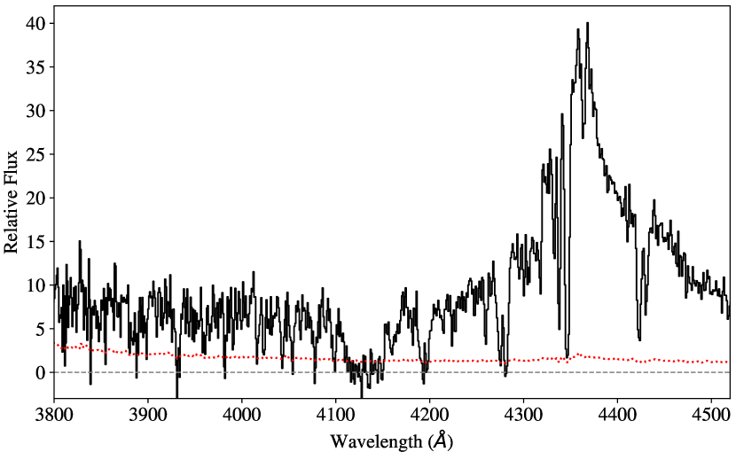
Figure 1 shows the SDSS spectrum of a DLA towards quasar J150321.87+323742.2 with emission redshift $z_{\rm em}=2.592$. These data have a spectral resolution FWHM $\approx 150$ km/s and a dispersion of $\delta\lambda\approx 1$Å per pixel. The broad and strong Ly$\alpha$ emission of the quasar, emitted at rest wavelength $\lambda_{\rm rest}=1215.67$Å in the quasar’s rest-frame, is apparent at an observed wavelength $\lambda_{\rm obs}=\lambda_{\rm rest}(1+z_{\rm em})\approx 4380$Å. The DLA occurs within the so-called Ly$\alpha$ forest, the thicket of absorption features blueward of the quasar’s Ly$\alpha$ emission due to hydrogen gas in the intervening, intergalactic medium at $z<z_{\rm em}$ (e.g. McQuinn, 2016). The DLA absorption is centered at $\lambda_{\rm obs}\approx 4130$Å giving an absorption redshift $z_{\rm abs}=\lambda_{\rm obs}/\lambda_{\rm Ly\alpha}-1\approx 2.397$. Although not covered in this spectrum, the DLA also exhibits higher order Lyman series lines including strong Ly$\beta$ absorption.

Traditional analysis of a DLA is to first estimate the unabsorbed quasar flux near $z_{\rm abs}$, referred to as the quasar continuum. One then estimates $z_{\rm abs}$ and $N_{\rm HI}$ for the DLA by comparing a model Ly$\alpha$ Voigt profile, which is the convolution of a Lorentz profile predicted by Quantum mechanics in the dipole approximation and a Gaussian profile assuming the gas satisfies a Maxwellian velocity distribution, to the absorption in the data. Errors in the $N_{\rm HI}$ value are estimated from the quality of the data, blending with the Ly$\alpha$ forest, and uncertainty in the continuum estimation.

A survey for DLAs repeats this analysis for many quasar spectra taking several considerations into account. First, one typically sets a minimum threshold on the signal-to-noise (S/N) of the spectra to insure confidence in the detection and analysis of the DLA profile. Previous human analyses of the SDSS quasar spectra have typically restricted to S/N $>4$, defined from the median flux of the data to the reported error array. Second, approximately 15% of luminous quasars exhibit strong associated absorption manifesting as broad absorption lines (BALs) in transitions of highly ionized species (e.g. OVI, NV). These BALs mimic DLAs and tend to compromise the spectrum for a DLA analysis. As such, they are generally ignored in DLA surveys.

Previous DLA surveys (e.g. Wolfe et al., 1995; Prochaska et al., 2005) have demonstrated that the incidence of DLAs is modest, e.g. $\approx 1$ in 4 SDSS spectra of $z>2.5$ quasars exhibit a DLA. One also finds that the distribution of $N_{\rm HI}$ values follows an $\alpha\approx-2$ power-law from column densities $\log N_{\rm HI}\approx 20.3-21.7$, which then steepens considerably at higher $N_{\rm HI}$.

Figure 1: SDSS spectrum of quasar J150321.87+323742.2 at $z_{\rm em}=2.592$ which exhibits an intervening DLA at $z_{\rm abs}\approx 2.397$ with $N_{\rm HI}\approx 10^{20.75}\,{\rm cm^{-2}}$ (Prochaska et al., 2005), which can be seen on the graph at the wavelength $\lambda_{\rm obs}\approx 4120$ Å.

Absorption systems with $N_{\rm HI}$ just below the DLA definition, i.e. $N_{\rm HI}\approx 10^{19.5-20.3}\,{\rm cm^{-2}}$, are commonly referred to as super Lyman limit systems (SLLSs) or sub-DLAs Prochaska et al. (2015). Uncertainty in the $N_{\rm HI}$ analysis implies a non-negligible number of SLLSs will be mis-classified as DLAs (by any approach). At low $N_{\rm HI}$, these are the primary contaminants in a DLA survey.

Figure 2: An outline of the neural network architecture used. See section 3 for a more detailed description. This is a standard convolutional neural network most commonly applied to image problems. We essentially cast DLAs as a 1D image problem.

3 Neural Network Model

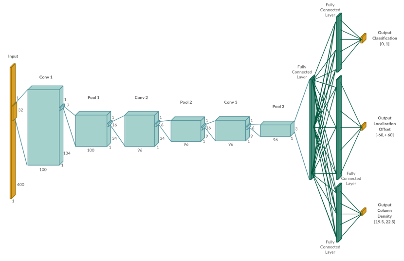
In this section we describe our neural network model. We use a standard 2D convolutional neural network architecture, but because a spectrum’s flux is a one-dimensional dataset, one dimension of the CNN is simply fixed at 1. An overview of the overall architecture is visualized in 965Figure 2.

3.1 Convolutional neural network architecture

Convolutional neural networks exploit spatial locality by enforcing a local connectivity pattern between neurons of adjacent layers. The architecture thus ensures that the learned filters produce the strongest response to a spatially local input pattern. Stacking many such layers leads to nonlinear filters that become increasingly global (i.e., responsive to a larger region of pixel space). This allows the network to first create representations of small parts of the input, then from them assemble representations of larger areas. In our case, this process allows the neural network to learn high level concepts such as measuring column density, rather than simply memorizing the input. As such, convolutional networks generalize to unseen samples very well.

Our neural network is constructed using a fairly standard CNN architecture (LeCun, 1989). First, three convolutional layers are constructed, each with a max pooling layer. A fully connected layer of size 350 follows the convolutional layers. Then follows the last layer that is comprised of 3 separate fully connected sub-layers, the outputs of which are used to perform 1) classification, 2) DLA localization, and 3) column density estimate, respectively. This last layer of multi-task learning is a novelty of our model (section 3.3).

The initial architecture started with classification only and evolved into three separate convolutional networks for the three outputs, each having hyperparameters tuned to achieve the best possible results. In experimentation we found that one network performed better on all three tasks than three individual networks. Our choice of three convolutional layers was initially arbitrary but experimenting with more layers did not improve results. All other hyperparameters were extensively optimized for, as discussed in section 4.3. The hyperparameters that govern the architecture and training of the network are tabulated in the Appendix (table LABEL:-table:hyperparameters).

We use the Adam (Adaptive Moment Estimation) algorithm to search for the optimal parameters for our neural network model (Kingma and Ba, 2015). Our neural network is implemented using Google’s deep learning framework TensorFlow (Abadi et al., 2015); and was trained on a server with two NVIDIA Tesla K20 GPUs.

3.2 Data input

The input to the neural network consists of the raw flux values in the sightlines. The uncertainty values (i.e. error array) are entirely ignored by the algorithm. Furthermore, no scaling was applied to the flux data. In fact, any attempt to perform typical zero-mean/unit-variance standardization, or to scale flux values to $(0,1)$ produced worse results than leaving them unscaled. Input values typically range from $\approx 0-50$ in the SDSS flux units of $10^{-17}\rm erg\,s^{-1}\,cm^{-2}\,\AA$.

We analyze a fixed range of the sightline ranging from 900Å to 1346Å in the quasar rest frame. The lower bound corresponds approximately to the HI Lyman limit in the rest-frame of the quasar. Below these wavelengths, intervening optically thick HI gas may greatly absorb the quasar and partially mimic the signal of a DLA. The upper bound of our analysis interval scans past the Ly$\alpha$ line to ensure DLAs on or near the Ly$\alpha$ emission line are recovered. From SDSS or BOSS spectra, this yields an input that is of size $[1748,1]$ (padded as necessary; see below), which are the dimensions fed to the neural network. Our first layer convolutional kernel is then $[32,1]$. This kernel size is much larger than the typical $[3,3]$ or $[5,5]$ kernel seen in most vision problems; we discuss how we chose this value and the hyperparameter selection process in detail in section 4.3.

We do not actually input all 1748 sightline pixels into our network because this would make identifying multiple DLAs along a given sightline too challenging. Therefore, the input to the network is a 400 pixel region of the sightline in a sliding window. For each sightline, the model performs 1748 separate inference steps with a 400 pixel window around every pixel of the spectrum producing a result. See the visualization aid in Figure 3.

The choice of 400 pixels was dictated by the width of DLA absorption ($\approx 10$Å in the DLA rest-frame) and the dispersion $\delta\lambda$ of the spectrometer ($\approx 1$Å for the SDSS and BOSS surveys). That is, we desired a window large enough to easily encompass a single DLA without greatly exceeding its width. Spectrometers with higher/lower dispersion would require a larger/smaller window. This means that the specific model described here is not directly applicable to datasets with different $\delta\lambda$, but we expect it will be straightforward to construct new models within a similar CNN architecture.

Figure 3: The sightline is broken into 400 pixel segments in a sliding window. An independent segment generates one prediction at each of the 1748 pixels in the sightline covering $900-1346$Å as the center point in the quasar rest-frame. This approach facilitates identifying overlapping DLAs and also generates a large training dataset.

3.3 Multi-task learning

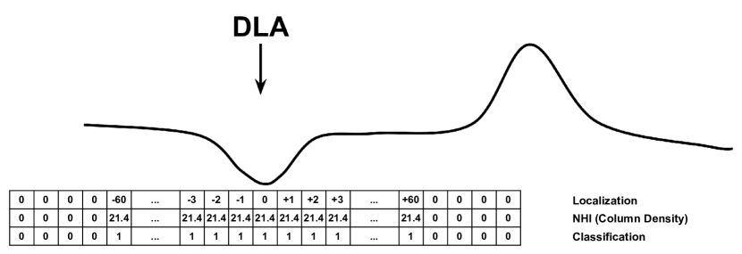
The network produces three outputs (labels) for every 400 pixel window in the spectrum. This multi-label approach is a novelty of the model and not a typical application of CNNs. The algorithm first classifies whether a DLA exists within 60 pixels of the center of a 400 pixel window. The value 60 was chosen as a range for which we can safely assume the DLA will be fully visible in the 400 pixel window. If a DLA is predicted the label takes on a 1/true value, else 0/false. Second the algorithm estimates the DLA line-center by producing a value in the range $[-60,+60]$ that indicates how many pixels the window center is from the center of the DLA. Third, the algorithm produces a column density estimate that is only valid if a DLA actually exists in the current window. A visualization of the labels for each pixel in a sightline is shown in Figure 4.

Our initial approach to the problem began with a simple CNN that identified sightlines with or without a DLA (simple binary classification). We then created a separate network that performed localization by improving upon the simple binary classification and outputting a predicted center point of the DLA relative to the current input. Finally we trained a third model to take the samples where a DLA exists somewhere in the window and trained it to predict the column density of the DLA, regardless of its location. We then found that combining the models into one multi-task learning model produced better results than training each model independently. Multitask learning refers to the concept that a learning algorithm, such as a neural network, may perform better when it is generalized to solve multiple (related) tasks. This is a method of regularization discussed in the Deep Learning Book by Goodfellow et al. (2016). With multi-task learning, we noticed an improvement in all metrics over the individually specialized models.

An astute reader will note that using a single model for all 3 of these outputs will force us to train on areas of sightlines where no DLAs exist. In these regions, the predictions for the column density measurement are irrelevant. We sidestep this issue by masking the gradient appropriately, as described in section 3.5.

Figure 4: A visual aid demonstrating the idealized labels for a DLA (not to scale). For any specific point taken as the center point of a 400 pixel window, the labels indicate: 1) the location (offset) of a DLA within that window or zero when no DLA exists, 2) the column density if a DLA exists in the window, or zero, and 3) a 1/0 classification indicating that a DLA exists.

3.4 Loss function for multi-task learning

In multi-task learning a model will produce multiple outputs for a given input. In our model, three outputs are produced: classification, localization, and column density estimation. Here we document the three individual loss functions, and the combined loss function which is optimized for. See figure 4 for a visual guide to the three labels we work with in these equations.

The loss function for DLA classification ($\mathcal{L}_{c}$) in a sample is the standard cross-entropy loss function:

$$\mathcal{L}_{c}=-y_{c}\log(\hat{y}_{c})-(1-y_{c})\log(1-\hat{y}_{c})$$ (1)

where $y_{c}$ is the ground truth classification label ($y_{c}=1$ if DLA; 0 otherwise) for the sample; and $\hat{y}_{c}$ is the model’s predicted classification ($\hat{y}_{c}$ is in the range (0,1) where $\hat{y}_{c}>0.5$ indicates a positive DLA classification and $\hat{y}_{c}<0.5$ negative classification).

The loss function for DLA localization ($\mathcal{L}_{o}$) is the standard square error loss function:

$$\mathcal{L}_{o}=(y_{o}-\hat{y}_{o})^{2}$$ (2)

where $y_{o}$ is the ground truth localization label in the range $(-60,+60)$; and $\hat{y}_{o}$ is the model predicted localization.

The loss function for log column density estimation ($\mathcal{L}_{h}$) is a square error loss function with gradient mask (see section 3.5):

$$\mathcal{L}_{h}=\left(\frac{y_{c}}{y_{c}+\epsilon}\right)(y_{h}-\hat{y}_{h})^{2}$$ (3)

where $y_{c}$ is the ground truth classification label (see eq. (1)); $y_{h}$ is the ground truth $\log N_{\rm HI}$ label ($y_{h}=0.0$ when no DLA exists, and in the range (19.5, 22.5) when a DLA exists); $\hat{y}_{h}$ is the model predicted $\log N_{\rm HI}$; and $\epsilon=10^{-6}$ is a small value safe from 32-bit floating point rounding error.

The final loss function for our multi-task learning model is the sum of the 3 individual loss functions:

$$\mathcal{L}=\mathcal{L}_{c}+\mathcal{L}_{o}+\mathcal{L}_{h}$$ (4)

We note that classification loss is not actually used in determining the existence of a DLA. We get better results by analyzing the models ability to predict the location of the DLA as we make predictions across the sightline. Classification loss proved to be a good regularizer for the network, improving the results of both localization and log column density estimates; this is its sole purpose.

3.5 Masking the gradient

There is a conceptual problem with the neural network described previously: on negative samples (those with no DLA in the 400 px window) the column density measurement has no meaning and the adopted label is 0.0. But if the model were trained to predict 0.0 when it classifies the regions with no DLA present, this would induce a bias towards 0.0 on positive samples because fully 50% of the training data (negative samples) would be spent predicting a column density result of 0.0.

To get around this problem, we mask the gradient of column density during training when the sample is negative. This is achieved by adding a mask term to the loss function for column density. The original loss function for column density is the standard square loss; we multiply this by a constant term that is 0 for a negative sample (no DLA) and 1 for a positive sample, see equation (3).

We multiply in the term: $\left(\frac{y_{c}}{y_{c}+\epsilon}\right)$ where $\epsilon=10^{-6}$, a value near zero that isn’t affected by 32 bit floating point rounding error. $y_{c}$ is the classification label of the sample. The multiplicative term will be approximately 1 when the label is non-zero, and approximately 0 when the label is 0 (i.e. a negative sample). During back propagation, this constant term will carry through to the derivative, zeroing it out.

The three loss functions are summed and the ultimate effect is that the column density loss does not contribute to the gradient for regions without a classified DLA. At inference time a column density value will be produced for negative samples by the model, but the value produced is simply ignored when no DLA is predicted and has no useful meaning. The idea of masking gradients is common to recurrent neural network implementations, but not commonly applied to feed forward or CNNs.

3.6 Overlapping DLAs

Because the incidence of DLAs is low, most spectra contain 1 or 0 systems. With a large enough dataset, however, sightlines with multiple DLAs occur and a subset of these will contain pairs of DLAs close in absorption redshift. We refer to these as “overlapping” DLAs. Labeling samples where two DLAs exist near each other or overlapping involves changing the localization and column density values such that they refer to the nearest DLA. This is a slight modification from what is seen in the visualization in Figure 4. For example if the center of two DLAs is 30 pixels apart, labels for localization would begin at $-60$, and continue to the first DLAs center with a localization label of $0$, then begin counting up to $+30$, at which point it would flip to $-30$ and count down again to the second DLA’s center with label $0$, and back up to $+60$. A similar approach is applied to column density. When calculating the column density measurement we normally average column density measurements across the $\pm 30$ values around the DLA center (see Section 5.1.4). When two DLAs overlap we make use of fewer column density measurements such that we use column density measurements up to the center point between the overlapping DLAs.

4 Training

4.1 Considerations

Figure 5 shows a sample spectrum and the positive (green), negative (red), and ignored (gray) regions. Notably there are far more negative regions than positive regions along the sightline. Training on more negative than positive samples would induce bias in the algorithm, so we balanced the positive and negative samples trained on. By design, our training dataset (described in 4.2) only contains sightlines with DLAs. In training we sample every possible positive samples from the sightline, and an equal number of negative samples are chosen from the sightline at random so that we maintain a 50/50 balance between training on positive and negative regions. This is standard practice in training such models.

Another issue arises at the boundary where a valid DLA is 61 pixels from the center of the window and the localization label abruptly changes from $\pm 60$ to 0. This would certainly cause trouble for the learning algorithm. Therefore, we do not train the model on these cases, and during inference we do not need the values at these edges to be accurate; they go unused and untrained.

We also ignore regions of the sightline where Ly$\beta$ absorption corresponding to identified DLAs takes place. The Ly$\beta$ absorption from DLAs may be falsely detected as Ly$\alpha$ from gas at lower redshift. The algorithm is not trained in a manner that would allow it to identify the difference between Ly$\alpha$ absorption and Ly$\beta$ absorption. Although this is potentially feasible, we did not include it in the scope of this work. We simply compute the Ly$\beta$ location and mask any identified absorption as Ly$\beta$ in post-processing (any corresponding strong HI absorber within 15Å of the predicted location of Ly$\beta$). Training on these regions would not stop the algorithm from learning, but lowers its accuracy by training on labels that indicate no absorption exists despite its presence. We do not train the algorithm on these regions, and remove them in post-processing at analysis time. While this reduces the spectral range searched for DLAs, the effect is small and eliminates a significant source of false positives from a DLA survey.

Figure 5: A colored representation of positive (green), negative (red), and ignored (grey) regions of the sightline. The green regions indicate training samples that have a DLA, the red regions are training samples that do not have a DLA, and the grey regions are excluded. The grey regions near the positive DLA are cases on the border between a DLA existing in the 400 pixel sliding window and not. The grey region at shorter wavelengths spans as the Ly$\beta$ absorption region of the DLA. For DLAs with high $N_{\rm HI}$ values, in particular, their Ly$\beta$ absorption mimics smaller DLAs and causes the training accuracy to decrease.

4.2 Training Set

In many respects, a CNN model is only as good as its training set and this bore true for our DLA analysis. Initially, we began with human-generated catalogs of DLAs (e.g. Noterdaeme et al., 2012) but found that these were too impure and too small ($N\lesssim 10,000$ DLAs) to train the CNN. We moved, therefore, to generate our own training set by inserting mock DLAs and SLLSs into SDSS spectra that were believed to have no DLAs.

Referring to the published survey of DLAs by Prochaska and Wolfe (2009), we identified the 4,113 sightlines that they analyzed which had no reported DLA, had a quasar redshift $z_{\rm em}>2.3$, a S/N greater than 5 measured from the median flux to error estimate near the quasar Ly$\alpha$ emission, and no BAL signature (flag=0). We will refer to these 4,113 sightlines as "DLA-free" and emphasize that they can and do include SLLS. We further note that this sample has higher S/N than a random sampling of $z>2$ SDSS quasar sightlines, i.e. our model is not trained extensively in the low S/N regime.

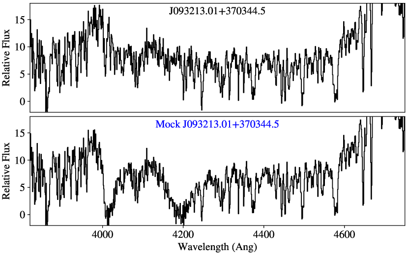
In several stages, we proceeded to generate 200,000 sightlines for training. For the first set of 135,000 sightlines, we drew emission redshifts uniformly from the range $z_{\rm em}=2.3-4.5$ and then matched it to the DLA-free sightline with smallest offset in $z_{\rm em}$. We then inserted at least one DLA into each sightline with column density drawn randomly from the $N_{\rm HI}$ frequency distribution of Prochaska et al. (2005) over the interval $\log N_{\rm HI}=20.3-22.5$. The absorption redshifts $z_{\rm abs}$ are constrained to place Ly$\alpha$ between 910Å and 1215Å of the quasar rest-frame. A Voigt profile was generated for each absorber and multiplied into the spectrum. This depresses the flux and also the noise fluctuations in the original data. Therefore, we added random fluctuations (with normal deviate) within the Voigt profile based on the error array of the spectrum and scaled by $1-f_{V}$ where $f_{V}$ is the normalized Voigt profile model. An example of mock-generated DLAs is shown in Figure 6.

To enable training on SLLS, we generated 45,000 sightlines as above but with systems having $\log N_{\rm HI}=19.5-20.3$. Lastly, we generated 20,000 sightlines with DLAs having $\log N_{\rm HI}=21.2-22.5$. This high $N_{\rm HI}$ sample improved the model’s ability to characterize the strongest DLAs. We note that these training spectra ignore several aspects of real data: (i) metal-line absorption; the majority of DLAs show strong, associated metal-line transitions including saturated SiIII 1206 absorption near Ly$\alpha$; (ii) any clustering of Ly$\alpha$ lines to DLAs as may be expected from hierarchical cosmology. We believe, however, that ignoring these effects has a minor impact on our results.

Training iterates through 100s of millions of data points, each being a random 400-pixel segment drawn from the above sightlines, also randomly chosen with the following exceptions: (i) the approximately 2,000 sightlines that have overlapping DLAs were sampled at $4\times$ the otherwise random rate to improve the algorithm’s ability to resolve these difficult configurations; (ii) the SLLS sightlines were sampled at half the rate as those with DLAs to limit their impact.; and (iii) positive/negative segments are selected at a rate of 50/50, i.e. we sample more densely from the positive regions of the sightline which are smaller segments than the negative regions (Figure 5).

Figure 6: (top) The SDSS DR7 spectrum of J093213.01+370344.5 which was characterized as DLA-free by Prochaska & Wolfe (2009); (bottom) the same sightline with two injected DLAs at $z_{\rm abs}\approx 2.303,2.450$ and with $\log N_{\rm HI}\approx 20.5,21.0$ respectively.

Lastly, 10,000 sightlines with at least one injected DLA (and no injected SLLS) were held for validation (see Section 5).

4.3 Hyperparameter selection

Hyperparameters were selected by identifying those that produce the best results on a held out validation dataset. There are 23 hyperparameters – everything from L2 regularization penalty to kernel sizes. All hyperparameters are listed in table LABEL:-table:hyperparameters. Hyperparameter selection was performed using a restricted coordinate descent method. Initially a reasonable value for the hyperparameters was configured manually. Then a number of values above and below this value were selected. We then randomly selected one hyperparameter and trained the network using each possible value for the hyperparameter. The value that yields the model with the best validation error is kept as the parameter value. We then choose a new hyperparameter and repeat the process until reasonable convergence (usually a day or two worth of training on our 3 layer convolutional network described in section 3.1). For hyperparameter search we ran training using two NVIDIA K20 GPUs to try different parameter combinations and limited the training to approximately 30 minutes, which was a reasonable trade-off between the final 1-2 day convergence and training time.

Through this process we were surprised by a few hyperparameter values. First, the number of filters selected for each layer of the network was very large. More than 100 filters in the first convolutional layer, for example, produced over-fitting. The batch size was a hyperparameter that was selected and the chosen value was clearly affected by the amount of data analyzed. When there was a large amount of data and over-fitting was less of an issue, a larger batch size produced better results. When we used smaller datasets a smaller batch size was used. The dropout keep probability and L2 regularization penalty behaved in a similar manner to batch size. Dropout was rendered all but ineffective as we grew the amount of data in our training set. The optimal kernel sizes of 32 and 16 were much larger than we had anticipated based on experience with image datasets where 3, 5, and 7 kernel sizes are common. The number of neurons in each fully connected layer was also subject to over-fitting when larger values were tested.

An unlisted hyperparameter that was originally tested is whether max pooling or mean pooling should be used. We never found a case where mean pooling outperformed max pooling and we eventually removed it as a hyperparameter.

5 Validation

To quantify the algorithm’s ability to properly identify and measure DLAs we compare it to two catalogs: one where we inject DLAs into real spectra believed to be DLA-free, and one manually analyzed by human experts on real data (Prochaska and Wolfe (2009)). Both of these datasets have the same selection criteria for quasar sightlines as the training set except being DLA-free. We analyze the accuracy in terms of (i) the detection rate of DLAs; (ii) the measurement precisions of $z_{\rm abs}$ and $N_{\rm HI}$; (iii) the rate of false negatives, DLAs known to exist a priori that were missed by the algorithm; and (iv) the false positive rate, DLAs that were identified by the algorithm but were not previously known.

5.1 DLA Analysis

We begin by describing the application of the CNN model to a single sightline for the identification and characterization of DLAs.

5.1.1 Preprocessing

The only preprocessing step on the spectral data is to pad the flux array on the left to create a fixed length sightline. This fills out each array to the same dimension but has no consequence to the algorithm. Padded values take on the mean of the first 50 pixels in the sightline, an arbitrary but effective choice.

5.1.2 Processing a Spectrum

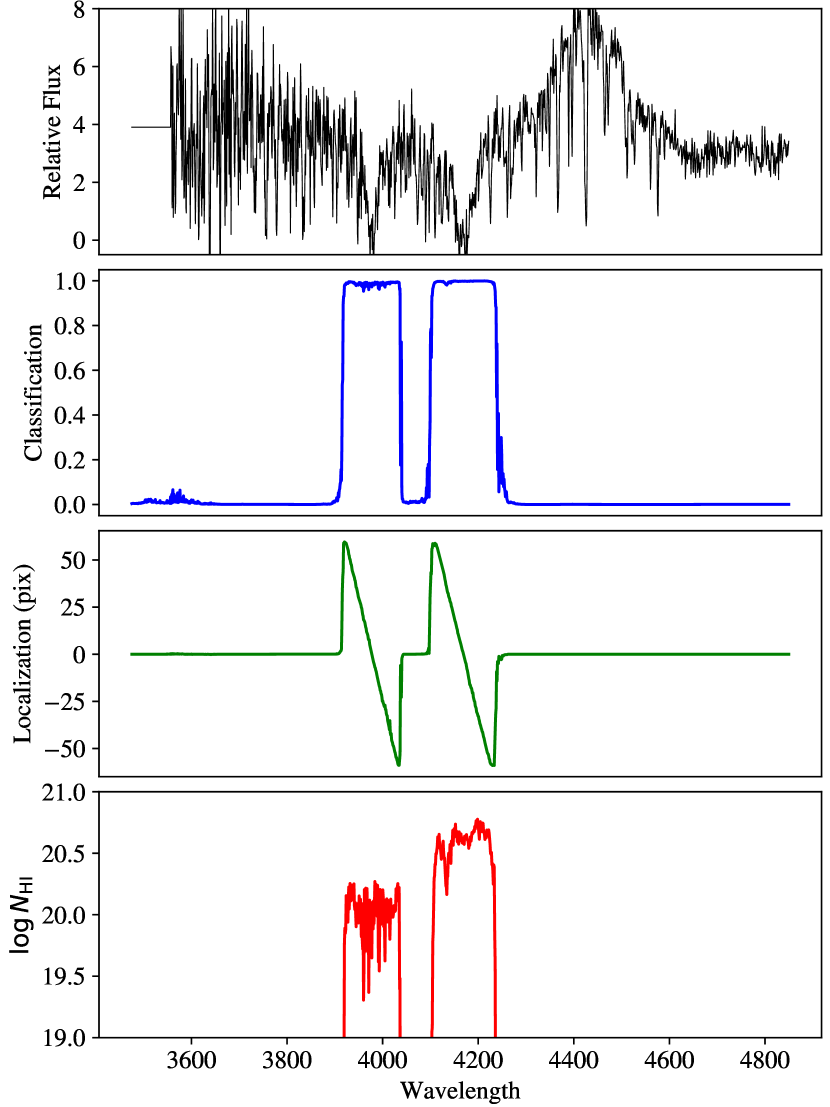
The spectrum fluxes are replicated into 1,748 segments of 400-pixels each. The neural network receives each 400 pixel segment and, for each segment, outputs three results: 1) A predicted classification in the range $(0,1)$ indicating whether a DLA exists within $\pm 60$ pixels from the center of the window; 2) an offset value from $[-60,+60]$ which indicates the relative location in pixels of the DLA to the center of the window (and 0 if the DLA is not within $\pm 60$ pixels of the center of the window); and 3) a logarithmic column density measurement ($\log N_{\rm HI}$). An example of the labels for a single sightline are shown in Figure 7. On a multi-core Intel based architecture, the algorithm process 500 spectra in approximately 140 s using 19 cores in parallel.

Figure 7: Example showing the labels along a single sightline. From top to bottom, the panels show: (i) the relative flux values for the spectrum; (ii) the classification labels; (iii) the localization labels; (iv) the $N_{\rm HI}$ labels. Note that the $N_{\rm HI}$ labels have no meaning (i.e. may be ignored) for spectral regions outside where a DLA has been classified.

5.1.3 Localization and Confidence

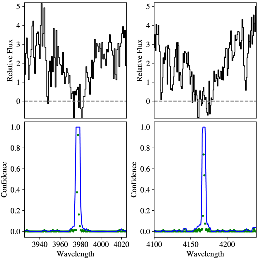
Given the model results for the full sightline, the next task is to identify the center location of any DLAs, i.e. the absorption redshift $z_{\rm abs}$. In the example given by figure 7, two DLAs were identified at $\approx 3980$Å and $\approx 4170$Å corresponding to $z_{\rm abs}\approx 2.27$ and 2.43. The full scan provides a set of offset values which we histogram, expecting to observe a cluster of values at the center of a bonafide DLA. These are shown in the lower panels of Figure 8 as green points, where the value indicates the fraction of the nearest 121 pixels ($\pm 60$) that indicate the DLA is located at this wavelength, scaled by 1.5 to bring typical values of true DLAs close to 1. We further define a confidence parameter where we sum the histogram over the nearest 5 pixels (i.e. $\pm 2$ pixels) and take a 9-pixel median filter of that result limiting its maximum value to 1. The choice of a 9-pixel kernel for the median filter is arrived at by balancing between over and under smoothing and determined by experimentation with the training set.

For well-localized DLAs, this confidence parameter shows a sharp peak, as seen in figure 8. The spectrum is then scanned for peaks with confidence exceeding a threshold of 0.2. Any such peak signifies a highly probable DLA candidate. We emphasize that the main results of this manuscript are insensitive to the choice for any threshold value within 0.2 and 0.7. We mask all pixels with confidence $>0.1$ that neighbor the DLA candidate, and then search for additional DLAs in the spectrum.

Figure 8: (top panels) Zoom-in snapshots of two DLAs classified in the spectrum shown in Figure 7. (lower panels) Colored dots show at each pixel the histogram of offset values within $\pm 60$ pixels that predict the DLA is located at the given pixel (scaled by an arbitrary 1.5 factor). The blue curve is the confidence parameter, the 9 pixel median of the histogram that is first summed in a boxcar of 5 pixels.

5.1.4 Column Density Measurement

As with localization, we analyze multiple predictions for the DLA $N_{\rm HI}$ value to derive the adopted value. When a DLA is identified, we take the 40 measurements of $\log N_{\rm HI}$ to the left and right of the DLA and average them. In this case the choice of 40 was a reasonable, but arbitrary number smaller than the $\pm$ 60 pixels used in localization/classification. The boundary at $\pm$ 60 pixels, where the label abruptly changes to 0, is expected to be problematic for training and we avoided that region. The bottom plot in Figure 7 shows log column density measurements around each DLA. One notes a modest variance to the measurements. By analyzing multiple measurements, this (1) reduces scatter in the algorithm’s prediction of log column density; and (2) the measured standard deviation gives a crude indication of the uncertainty in the $N_{\rm HI}$ value.

In all previous human-led works, column density measurements of DLAs were derived from fits of a Voigt profile. Our approach with deep learning, however, does not explicitly implement any concept of Quantum Mechanics yet yields excellent results. We suspect, however, that the algorithm learns by matching patterns such as the shape of the wings inherent in a Voigt profile to map to real-valued column density output.

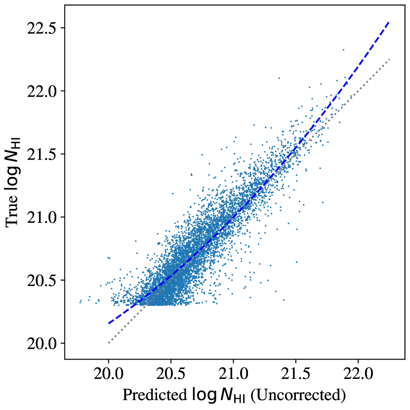
The algorithm does exhibit a small consistent bias at the high and low end of $N_{\rm HI}$ values which we characterized using a 5,000 sample validation dataset. A plot of the column density predictions and actual values on this validation dataset can be seen in Figure 9. This distribution of bias is consistent across both generated and human tagged datasets. For the final measurements, and those reported here, we fit the bias with a simple 3rd degree polynomial ridge regression model, and add the bias from all samples. The 4 ridge regression coefficients are: $f(x)=0.0028149x^{3}-0.06461880x^{2}-0.004256562x+23.5553179$, where $f$ is the amount of bias to remove from the models estimate, and $x$ is the biased column density estimate from the model.

Figure 9: Scatter plot of actual column densities of injected DLAs versus the uncorrected $N_{\rm HI}$ value predicted by the algorithm. The gray dotted curve is the one-to-one line marking a perfect prediction. The blue dashed-line is a 3rd degree polynomial ridge regression fit to the points, showing a small negative bias, more pronounced at the large and small extremes. This fit is applied to all predicted $N_{\rm HI}$ values.

5.2 Comparing results against a generated catalog

The results listed in this section report on the algorithm’s ability to identify and measure DLAs for which we know $z_{\rm abs}$ and $N_{\rm HI}$ exactly. Specifically, we analyzed 10,000 sightlines from the training set that were held out. Each sightline in this dataset contains 1 or more artificially injected DLAs ($\sim$87% have 1 DLA, $\sim$12% have 2 DLAs, $\sim$1% have 3 DLAs, and only a few have 4 DLAs), for a total of 11,403 generated DLAs.

5.2.1 Matched DLAs

To match our algorithm-predicted DLA with those injected, we require the predicted absorption redshift lie within $\delta z=0.015$ ($\approx 1200\,\rm km\,s^{-1}$) of the true value. With this $\delta z$ criterion, the algorithm successfully recovered 11,110 DLAs from the test set, i.e. 97.4%. Furthermore, an additional 184 of the true DLAs were classified by the algorithm as an SLLS (i.e. a system having $\log N_{\rm HI}<20.3$). This is expected and gives an overall strong HI absorber yield of 99%.

For the 11,110 matched DLAs, we measure a median $\delta z$ of $-0.00037$ ($\approx-30$ km/s) and a standard deviation of $\sigma(\delta z)=0.0022$. The distribution of log column density difference $\Delta N_{\rm HI}\equiv\log N_{\rm HI}^{\rm true}-\log N_{\rm HI}^{\rm model}$ forms a Gaussian distribution with mean 0.031 and standard deviation of 0.15 dex.

5.2.2 False Negatives

In the 10,000 sightlines tested, a total of 299 injected DLAs were not identified as a DLA by the algorithm. Figure 10 shows a scatter plot of $z_{\rm abs}$ and $N_{\rm HI}$ for these false negatives on a 2D histogram of the entire injected distribution. Approximately 2/3 of the false negatives were classified by the algorithm as an SLLS (i.e. with $\log N_{\rm HI}<20.3$) almost all have a truly low $N_{\rm HI}$. This behaviour is both expected and reasonable.

Figure 10: Scatter plot of $z_{\rm abs}$ versus $N_{\rm HI}$ for the false negatives from the 10,0000 sightline validation set. The underlying gray histogram illustates the distribution of $z_{\rm abs}$,$N_{\rm HI}$ pairs for the full, injected sample of 11,143 DLAs. Approximately 2/3 of the false negatives are characterized as SLLS by the algorithm and have true $\log N_{\rm HI}<20.5$ dex. The false negatives that were ‘missed’ by the algorithm (red squares) includes a set of $\approx 20$ systems with large, true $N_{\rm HI}$ values. See the text for a discussion of these which are dominated by overlapping DLAs.

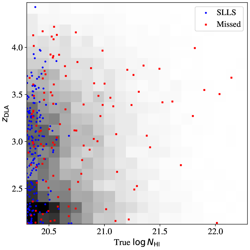
The remaining 115 cases of false negatives that were missed by the algorithm occur for a number of reasons. The dominant cause is overlapping DLAs, i.e. two or more DLAs with nearly coincident redshift. As is apparent from Figure 10, the missed DLAs are biased towards high $N_{\rm HI}$ value. This results from the fact that the algorithm occasionally mis-classifies (i) an injected DLA with high $N_{\rm HI}$ as two or more DLAs; (ii) a pair of injected DLAs as a single DLA; and (iii) a pair of injected DLAs as two offset DLAs. Examples of the first two cases are shown in Figure 11.

While the algorithm properly predicts overlapping DLAs in the majority of cases, there are still a non-negligible incidence of mis-classifications. Of course, human-based approaches are also prone to this issue. These high $N_{\rm HI}$ false negatives constitute 20 of the 1200 injected DLAs with high value ($\approx 2\%$). We consider this an acceptable rate but will consider a larger training set of DLAs with high $N_{\rm HI}$ to (hopefully) improve learning on these systems.

Figure 11: (top) An example of two overlapping DLAs (marked by green dotted lines) generated as part of the training and test datasets, which the algorithm erroneously identified as one DLA (blue, dashed line). Note that the total $N_{\rm HI}$ value predicted is comparable to the sum for the pair of DLAs. (bottom) An example where the algorithm predicted that a single, injected DLA is a pair of overlapping DLAs. Both of these cases lead to false positives and negatives in the analysis.

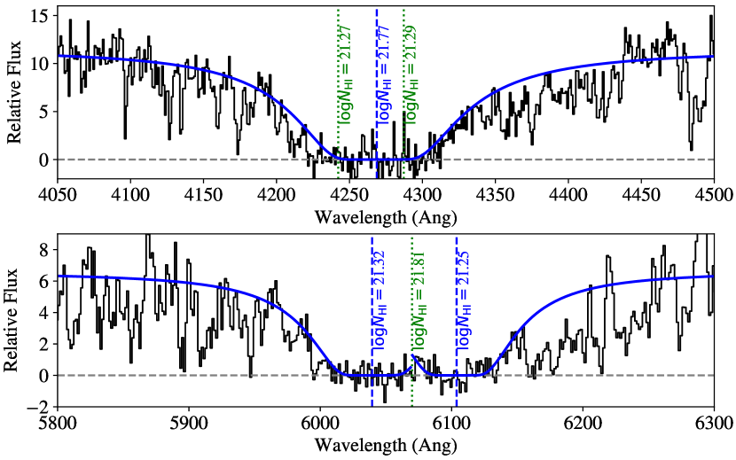
The next most frequent cause of missed false negatives was for DLAs injected within the noisy end of the spectrum, i.e. typically below $\approx 4000$Å. The failures here have a lower signal to noise ratio, and in many cases even a human expert would struggle to identify the DLA. By the same token, we identify examples where the algorithm successfully identifies a DLA in S/N$<2$ per pixel conditions (Figure 12). Our assessment is that the algorithm performs at least as well as a human expert in these low S/N cases.

Completing the census of false negatives, there were 8 cases in which an injected DLA overlapped a Ly$\beta$ absorption and was ignored. Such cases will exist in real datasets and are an unavoidable issue. In six other cases the algorithm did in fact identify the DLA, but failed to measure its center point to within $\delta z=0.015$. Finally there are three cases where the algorithm ignored the injected DLA for non-obvious reasons.

Figure 12: Two examples where a DLA was manually injected into a low S/N region of spectra and correctly identified by the algorithm. Very few humans would confidently identify either of these systems.

5.2.3 False Positives

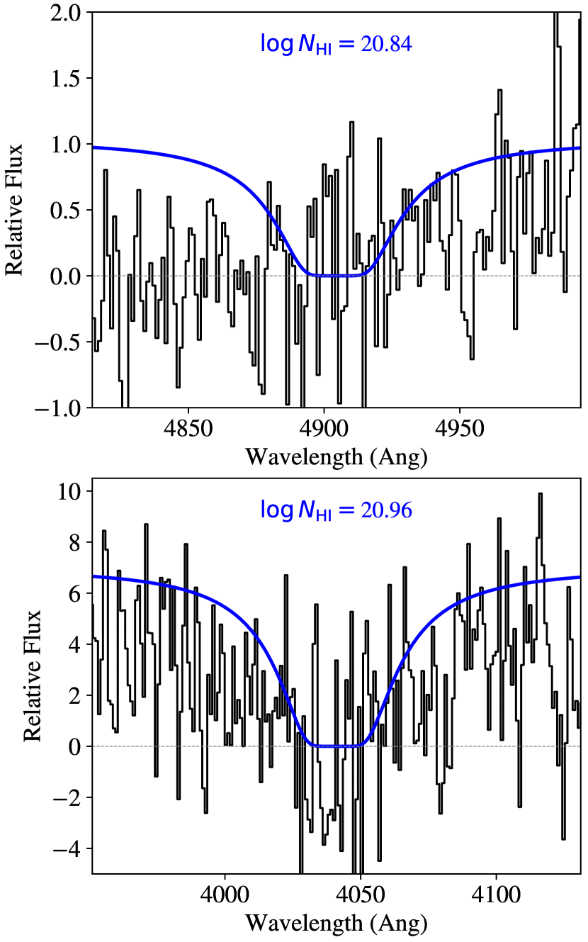
Generally, a false positive is defined as a reported DLA that does not match any injected DLA. By that definition, the algorithm identified 158 DLAs without a match within $\delta z=0.015$ to the injected sample. However, the DLA-free SDSS sightlines used to build the training set may include DLAs in the spectral region not surveyed by Prochaska and Wolfe (2009). These are the bluest, lowest S/N regions of the spectra. Indeed, 83 of these putative false positives fall within these non-surveyed spectral regions and a visual inspection reveals that many ($>40$) are likely legitimate DLAs. Therefore, we restrict our definition of false positives in this validation as those within the statistical Prochaska and Wolfe (2009) survey.

With this definition, 74 false positives were identified in this dataset of 10,000 test sightlines with 11,143 injected DLAs. Of these, only 1/3 have a high confidence value ($>0.9$). We have manually inspected these 74 false positives and have categorized them as follows: 31 cases have low $N_{\rm HI}$ values (i.e. near the DLA threshold) and it is possible that a fraction of these are legitimate DLAs. Indeed, many of these are listed within the DR5 catalog of Prochaska and Wolfe (2009) as SLLSs. A few typical examples of these false positives are shown in figure 13.

Figure 13: Examples of typical false positives in the generated validation set. The majority of appear to be bonafide DLAs in the purported DLA-free sightlines of Prochaska & Wolfe (2009); very few are egregious errors of the algorithm.

Another 25 of the false positives are due to errors related to overlapping DLAs with one or both having high $N_{\rm HI}$. Approximately half are cases where the algorithm identifies a single injected DLA as two absorbers and the other half are two injected DLAs reported as single one with a significantly offset redshift (Figure 11). The remainder result from a miscellaneous range of errors (e.g. a strong Ly$\beta$ line misidentified as a DLA) with only a few egregious cases. The false positive rate reported here is very low, but we caution that this validation set did not include injected SLLS which would increase the rate.

5.3 Generalizing to real-world data: DR5

Our algorithm performed well on the 10,000 sample test set, drawn from the distribution of sightlines used for training. This might, however, be considered too idealized of a test for validation. To further test our algorithm, we examined how the same model generalizes to real-world sightlines. Specifically, we analyzed the same SDSS sightlines surveyed by Prochaska and Wolfe (2009) and restricted to their statistical sample of DLA. We further limited our analysis to the SDSS DR7 quasar spectra catalog provided in the igmspec database (Prochaska, 2017) which eliminates five sightlines from Prochaska and Wolfe (2009). Altogether, this validation set includes 737 DLAs in 7477 sightlines.

5.3.1 Results for Matches

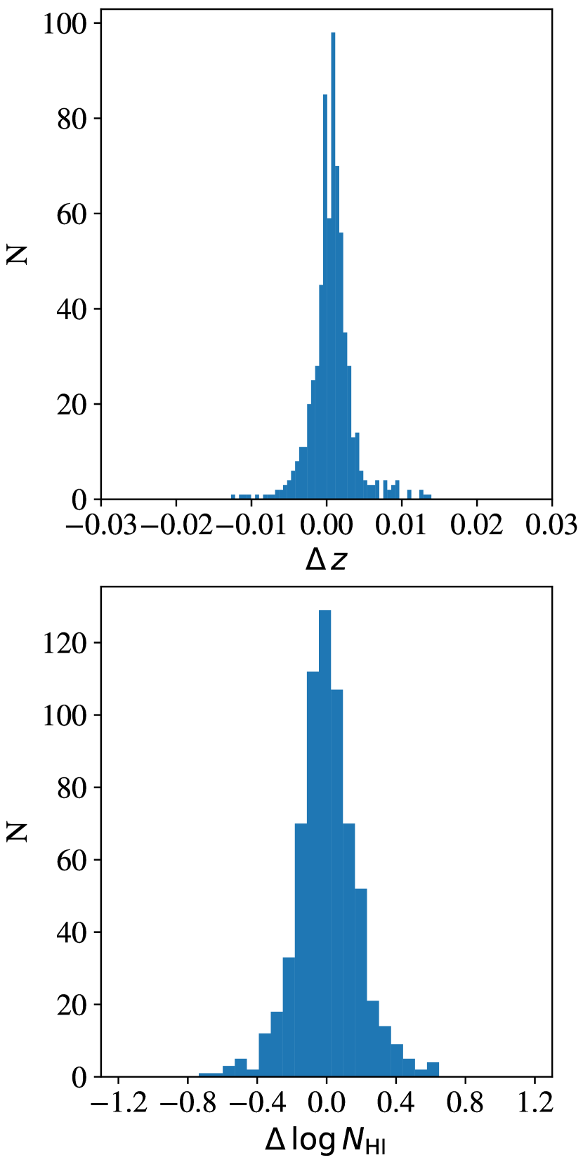
Our algorithm predicted a DLA matched to within $\delta z=0.015$ for 670 of the 737 statistical DLAs of Prochaska and Wolfe (2009). Figure 14 shows histograms of the offsets in redshift and $N_{\rm HI}$ between the algorithm’s predictions and the Prochaska and Wolfe (2009) values. The median redshift offset is only 0.0007 with a standard deviation of 0.0028. The median log column density offset is $\Delta N_{\rm HI}=-0.006$ with standard deviation of 0.18 dex, quite similar to the generated training and test datasets.

Figure 14: Redshift (top) and $N_{\rm HI}$ (bottom) offsets for the DLAs matched between the algorithm and the human-identified DLAs in the SDSS DR5 (Prochaska and Wolfe, 2009). The rate of DLA recovery by the algorithm is very high ($>95\%$) and the accuracy in $z_{\rm abs}$ and $N_{\rm HI}$ is excellent.

5.3.2 False Negatives

False negatives are defined as DLAs in the statistical DLA sample of Prochaska and Wolfe (2009) that were not identified by the algorithm. There are 67 such cases and 49 of these were reported by the algorithm to be an SLLS. These false negatives are expected and the rate is consistent with expectation. The remaining 18 are a combination of redshift offset $\delta z>0.015$, overlapping DLAs, and several egregious misidentifications. Allowing for the 49 SLLSs, the algorithm discovered a total of $719/737\approx 97.6\%$ strong HI absorbers from the set of human-identified DLAs.

5.3.3 False Positives

False positives account for cases when the algorithm identifies a DLA that was not previously labeled in the DR5 dataset. As with the test set, we restrict the definition to DLAs in the spectral regions surveyed for DLAs by Prochaska and Wolfe (2009). i.e. regions that satisfied their S/N threshold. There are 191 false positives that fell within the range analyzed by Prochaska and Wolfe (2009). Of these, 111 have $\log N_{\rm HI}\ \leq 20.45$, i.e. near the DLA threshold which may well be true DLAs. Because these false positives outnumber the false negatives, this could indicate a several percent underestimate in the incidence of DLAs by Prochaska and Wolfe (2009).

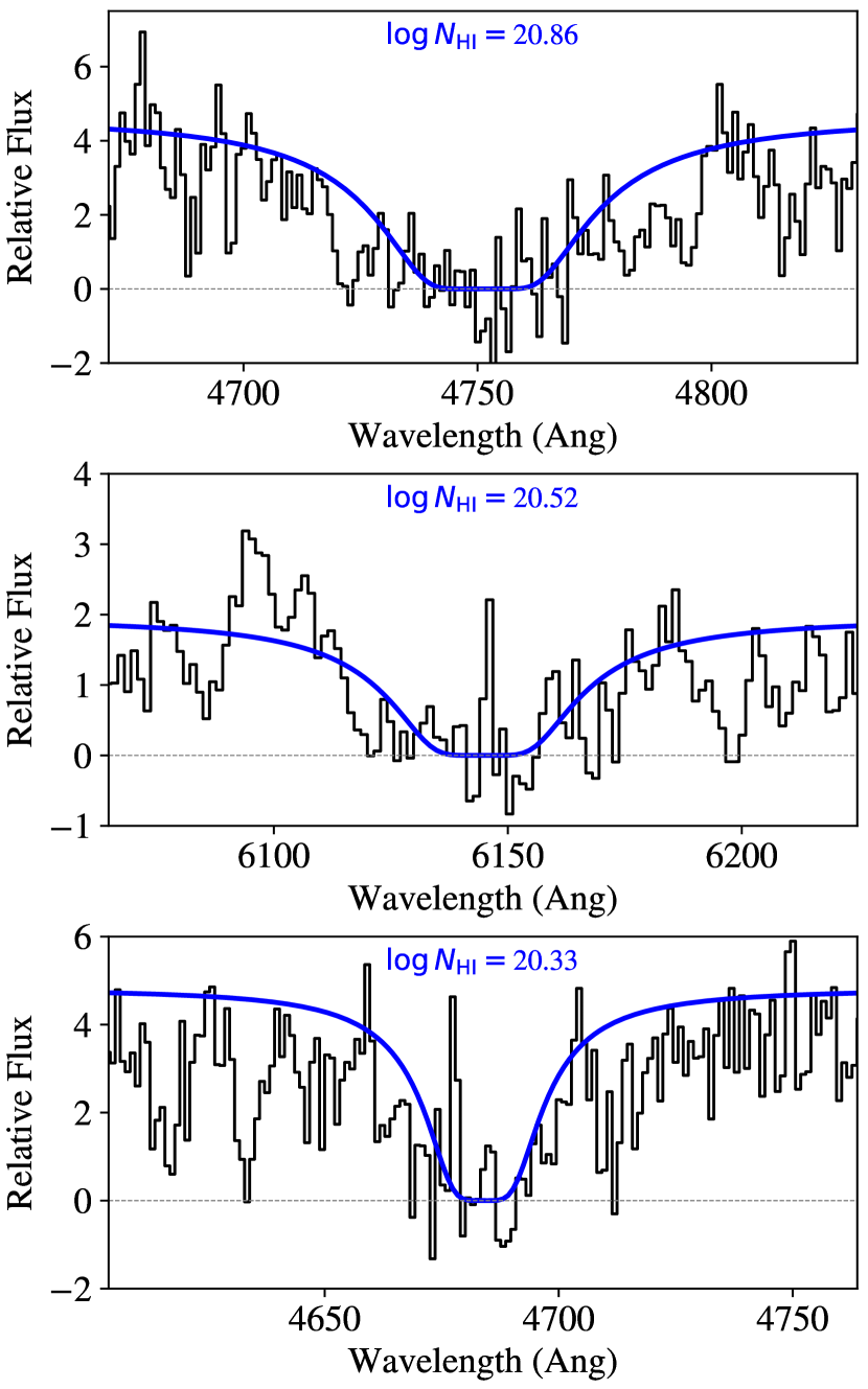
There were six false positives with $\log N_{\rm HI}>21$ which we examined closely. Three of these are obvious DLAs that were not reported by Prochaska and Wolfe (2009) for unknown reasons ($!$) and two are proximate DLAs. The sixth occurs at $z\approx 5$ in a noisy spectrum and is likely erroneous. There are 35 false positives with intermediate $N_{\rm HI}$ values ($20.6<\log N_{\rm HI}<21$). Of these, 27 occur along sightlines with $z_{\rm em}>3.8$ and lower S/N spectra. By human inspection, most are plausible candidates but we suspect the algorithm is over-predicting the incidence. The other eight are high quality systems that were missed by Prochaska and Wolfe (2009).

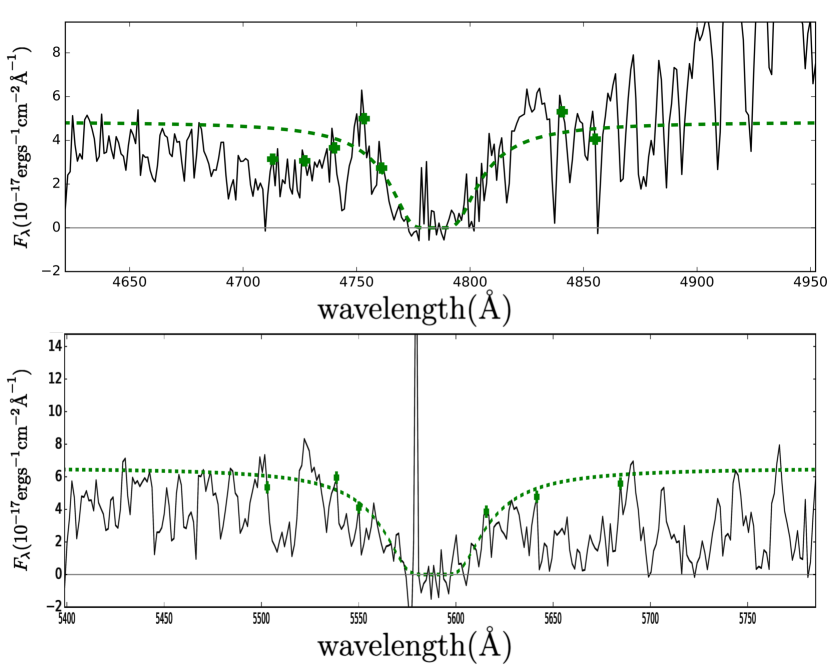
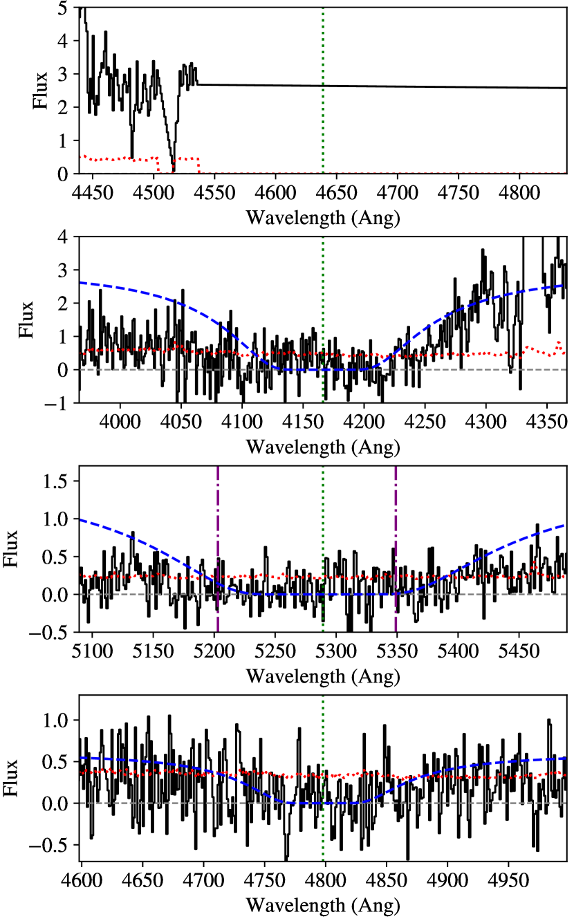
We highlight a particularly interesting false positive case where the algorithm identified a DLA that at first glance looks to be in error. In figure 15 a DLA is identified in the DR5 dataset despite a notably significant positive flux in the middle of the DLA. The SDSS DR5 catalog did not indicate any error with this flux, and thus we first considered the DLA to be a false positive. However analyzing this same sightline in the BOSS-DR12 dataset reveals that the flux at $\lambda\approx 4778$Åin the SDSS spectrum was spurious and that a true DLA is present! This is notable because these cases are learned, the algorithm identified a DLA in this case because there are examples of night sky flux in the training samples.

Figure 15: Above: Sightline from DR5 (plate 2111, fiber 525) with a reportedly relevant flux in the middle of the DLA which is identified as a DLA only by the algorithm. Below: An example from training data with night sky flux coincidentally part of the DLA. This absorption was also properly identified as a DLA by the algorithm.

Figure 16: Three DLAs reported by the machine learning algorithm that were not previously reported in prior SDSS DLA surveys. The top two cases also show strong, coincident low-ion absorption outside the Ly$\alpha$ forest. All three quasars were also observed in the BOSS survey and those data all support their characterization as DLAs.

6 SDSS-DR7 DLA Catalog

Buoyed by the results from our validation tests, including the comparison to real world data analyzed by human experts, we applied the CNN model to the entire SDSS DR7 quasar catalog. Specifically, we analyzed the 24,740 spectra of quasars with $z_{\rm em}>2$ from the Schneider et al. (2010) catalog provided by the igmspec v2 database. Table 1 provides the catalog of DLA candidates reported by the algorithm including a flag for BAL classification taken from Shen et al. (2011) and restricting to systems with $z_{\rm abs}<z_{\rm em}$. There are 4,913 candidates with $z_{\rm abs}<z_{\rm em}$ in quasar sightlines not flagged as a BAL, but we caution that our own visual inspection indicates a non-negligible fraction of these quasars show associated absorption that mimic DLAs. If we further restrict to systems with a confidence parameter $>0.9$, there are 2,714 high-confidence DLAs in non-BAL quasar sightlines.

Noterdaeme et al. (2009) have performed their own human+algorithm based survey of the SDSS DR7 quasar spectra. Matching their sample of 937 DLAs to ours within $\delta z=0.015$, we report 777 of these as DLAs and 45 as SLLS. For the matched DLAs, we find the $N_{\rm HI}$ values of Noterdaeme et al. (2009) are systematically higher then our algorithm’s by $\approx 0.07$ dex with a standard deviation of 0.17 dex. We visually inspected the 17 ‘misses’ with $\log N_{\rm HI}>20.8$. Eight are offset by more than 0.015 in redshift with neither algorithm showing systematically superior results. Seven from the Noterdaeme et al. (2009) survey are not DLAs (e.g. the purported system at $z_{\rm abs}=3.563$ toward J114317.14+142431.04) or at best ambiguous. There is one egregious miss (at $z_{\rm abs}=2.88$ towards J133042.52-011927.55) which we then realized is also absent in the Prochaska and Wolfe (2009) survey. Therefore, this spectrum was part of our DLA-free training set and we expect the algorithm learned to mis-classify it. Lastly, there is one example with apparent flux in the core of Ly$\alpha$ (at $z_{\rm abs}=3.553$ toward J205509.49-071748.62) which is bonafide and not recovered by our algorithm (nor Prochaska and Wolfe (2009)).

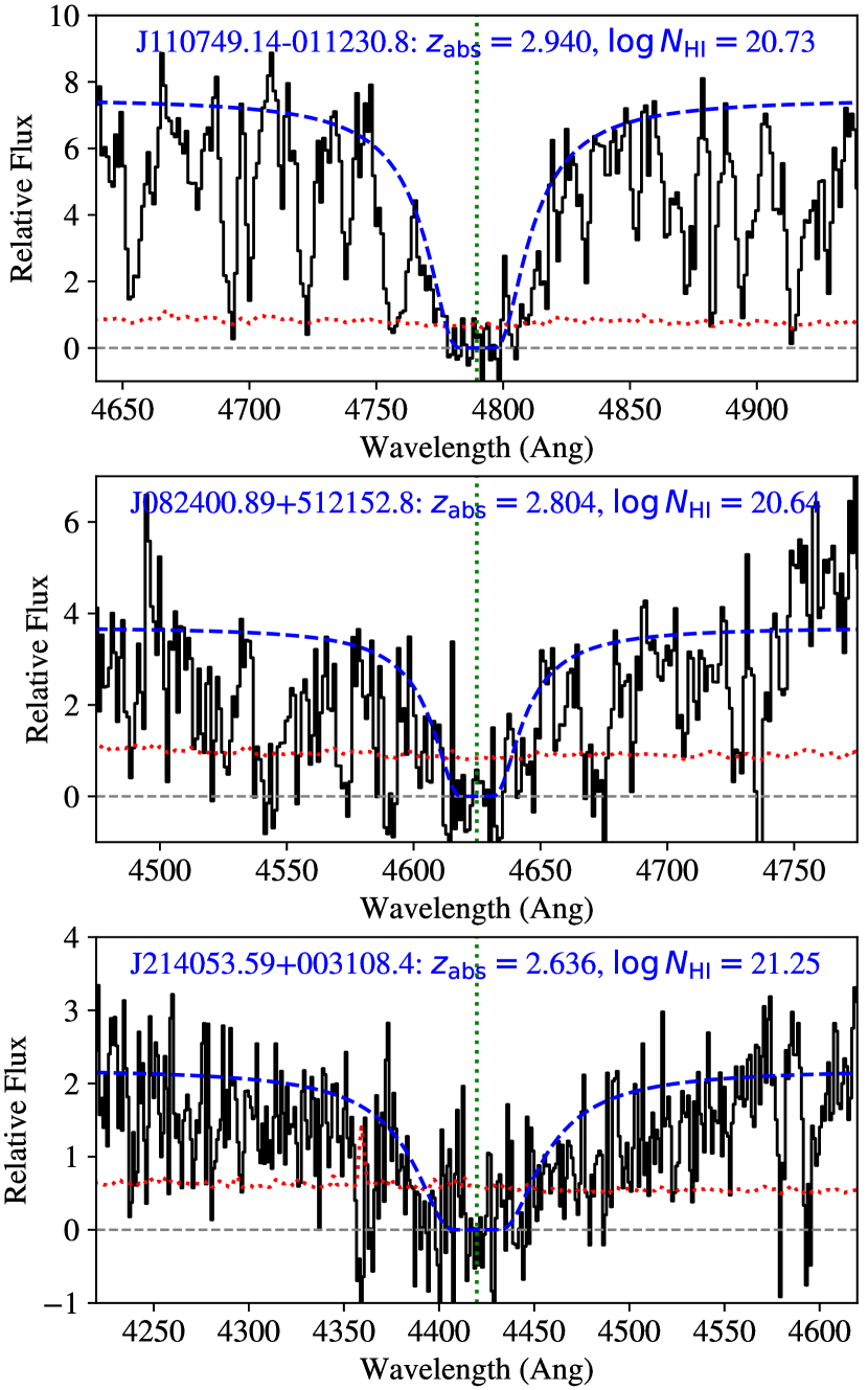
Altogether we report 1,659 DLAs in the DR7 with confidence=1 that are not listed in Prochaska and Wolfe (2009) nor Noterdaeme et al. (2009) (including over 1,000 at $z_{\rm abs}<3.5$ where blending in the IGM is less severe). We have visually inspected $\approx 100$ of these and find the majority are in lower S/N data and are highly plausible DLAs (e.g. a high fraction exhibit corresponding, strong low-ion metal absorption). Figure 16 shows several examples with $N_{\rm HI}>10^{20.5}\,{\rm cm^{-2}}$. Approximately 10% of these high-confidence DLA candidates are mis-identified associated absorption for quasars not previously deemed a BAL. Because Noterdaeme et al. (2009) did not publish their survey path for DLAs, we cannot determine whether any of the additional DLAs discovered by our algorithm would affect their statistical results.

Table 1: SDSS DR7 DLA CANDIDATES^a

RA	DEC	Plate	Fiber	$z_{\rm abs}$	$N_{\rm HI}$	Conf.	BALb	Previous?c
145.9092	-1.0054	266	124	2.322	20.41	0.47	1	0
147.0957	0.9318	266	617	3.431	20.38	0.39	0	0
151.1185	0.3071	269	467	2.540	20.95	0.94	0	3
151.1185	0.3071	269	467	2.685	20.95	1.00	0	3
154.6352	0.2434	271	500	2.606	20.48	0.82	0	0
154.6352	0.2434	271	500	3.714	20.43	1.00	0	0

^aRestricted to systems with $z_{\rm abs}<z_{\rm em}$.
^bQuasar is reported to exhibit BAL features by Shen et al. (2011) (1=True). We caution that additional BAL features exist in the purported non-BAL quasars.
^cDLA is new (0) or is also reported by N09 (1), PW09 (2), or both (3).

7 BOSS-DR12 DLA Catalog

A principal motivation of this work was to apply a machine learning algorithm to the complete DR12 dataset. Using the same model derived from the SDSS DR5 training set and applied to the SDSS DR7 quasar spectra, we derive DLAs from the BOSS DR12 dataset provided in igmspec, v2. Specifically, we analyze the 201,776 spectra for quasars with $z_{\rm em}>1.95$ including sources with BALs.

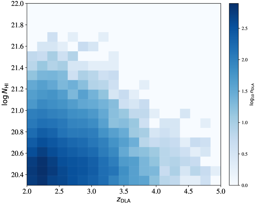
The model reports 50,969 systems with $\log N_{\rm HI}\geq 20.3$, $z_{\rm abs}>2$, and $z_{\rm abs}<z_{\rm em}$ in the 174,691 sightlines not flagged as BALs in the BOSS quasar catalog (Table 2). A 2D histogram of the $N_{\rm HI}$ and $z_{\rm abs}$ values is shown in Figure 17 for the subset (18,959) with high confidence (confidence $>0.9$). This relatively pure sample constitutes a several-fold increase over any previously published catalog.

Figure 17: 2D Histogram of the $z_{\rm abs}$, $N_{\rm HI}$ distribution of DLAs reported by the CNN algorithm for the set of BOSS DR12 quasars. Sightlines are restricted to those without strong BAL features. The DLAs are restricted to $z_{\rm abs}>2.$, $z_{\rm abs}<z_{\rm em}$, and confidence $>0.9$. There are a total of 18,959 DLAs satisfying these cuts.

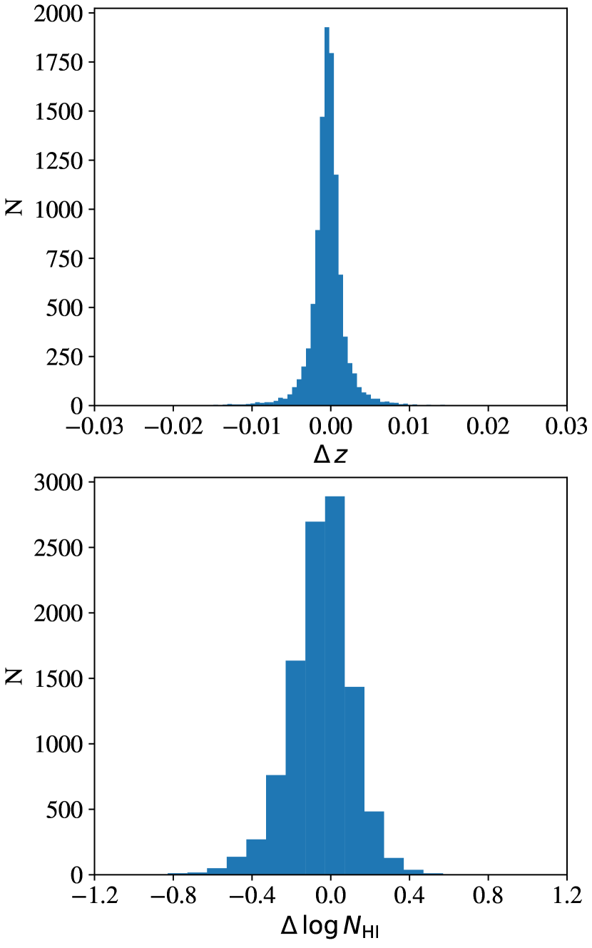
As described in the Introduction, Garnett et al. (2016) have developed their own ‘big data’ algorithm to process BOSS DR12 quasar spectra to assess the likelihood of intervening DLAs. Matching to $\delta z=0.015$ tolerance, we find that 10,571 of our pure sample are tabulated in Garnett et al. (2016) with nearly all occurring in a sightline reported by those authors to be highly confident to contain a DLA (pDLAD $>0.9$). Approximately 40% of the 8,388 non-matched DLAs occur blueward of Ly$\beta$ in the quasar rest-frame, which was outside the catalog provided by Garnett et al. (2016). Restricting to quasar rest-frame wavelengths $\lambda_{\rm rest}>1030$Å and to DLAs with $\log N_{\rm HI}>21$ (which one expects to be sufficiently strong to detect in any algorithm), there are 71 systems not matched. We have inspected a subset to verify few (if any) are egregious errors in our algorithm. Most are either in sightlines with 2 or more DLAs (also not classified by Garnett et al. (2016)) or proximate to the quasar. Figure 18 compares the absorption redshifts and $N_{\rm HI}$ values between the matched DLAs from the two algorithms. We measure small median offsets of $\Delta z=-0.00035$ and $\Delta N_{\rm HI}=-0.038$ and standard deviations of 0.002 and 0.16 dex respectively.

Figure 18: Histograms showing the differences for (top) $z_{\rm abs}$ and (bottom) $N_{\rm HI}$ between DLAs recovered by our deep learning algorithm matched to systems predicted by Garnett et al. (2016). For these 10,571 matched DLAs, the estimated properties are in excellent agreement.

Reversing the matching process, i.e. comparing the results of Garnett et al. (2016) to our CNN algorithm, we find that $\approx 2,000$ of the DLAs in high probability sightlines are not matched to our algorithm. Many of these have $N_{\rm HI}$ close to the DLA threshold but 408 have $\log N_{\rm HI}>21$. We have examined $\approx 100$ of these cases by inspecting the BOSS DR12 spectra at the purported DLA position and also searched for associated metal-line absorption. There is a small, subset of cases where the ‘best’ model from Garnett et al. (2016) is very likely in error (e.g. bad data, pairs of DLAs, significant flux in the DLA core; Figure 19). The majority, however, correspond to low S/N spectra which exhibit a broad depression in flux at the putative DLA which may well result from a high $N_{\rm HI}$ system. Our algorithm, which was not extensively trained on very low S/N spectra, did not classify these cases as DLAs. There is an additional set of high-$N_{\rm HI}$ misses that differ in $z_{\rm abs}$ by more than 0.015 and less than 0.05. A search for corresponding metal-line absorption near $z_{\rm abs}$ shows cases where the model from one or the other algorithm is preferred and also cases where both are significantly offset. Lastly, there are a few cases (e.g. at $z_{\rm abs}=3.626$ toward J150731.89+435429.7) where the Garnett et al. (2016) algorithm has identified a very strong DLA in low S/N spectra that was missed by the CNN.

Table 2: BOSS DR12 DLA CANDIDATES^a

RA	DEC	Plate	Fiber	$z_{\rm abs}$	$N_{\rm HI}$	Conf.	BALb	G16c?
8.4806	-0.0140	3586	158	2.098	20.45	0.84	1	0
7.7251	-0.0462	3586	320	2.131	20.56	0.99	0	0
7.8980	0.7510	3586	728	2.125	20.31	0.45	1	0
8.3262	0.2714	3586	816	2.478	20.30	0.78	0	0
9.8449	-0.7361	3587	100	2.163	20.63	1.00	0	1
9.7215	-1.0555	3587	130	2.150	20.71	0.21	0	0

^aRestricted to systems with $z_{\rm abs}<z_{\rm em}$ and $z_{\rm abs}>2$.
^bQuasar is reported to exhibit BAL features by the BOSS survey.
^cDLA is new (0) or reported by G16 (1).

Figure 19: Example BOSS DR12 spectra at the location of several, high $N_{\rm HI}$ DLAs reported in Garnett et al. (2016) which appear to be in error. The top panel is a case of missing data, the 2nd panel has significant flux in the purported DLA core (a DLA may be present at higher $z_{\rm abs}$), the 3rd panel shows an example where there are two DLAs (confirmed by metal-line absorption), and the bottom case is a low S/N example with apparent residual flux.

8 Concluding Remarks

In this manuscript, we have applied deep learning techniques on astronomical spectra to classify and characterize the distinct spectral features known as damped Ly$\alpha$ systems (DLAs). Our fully-automated algorithm efficiently and precisely identifies DLAs and estimates their absorption redshifts and HI log column densities, with high efficacy. The results, as best we can assess, are as reliable and robust as any previous human-generated analysis. The algorithm struggles in several domains (e.g. overlapping and/or very high $N_{\rm HI}$ DLAs) and frequently misidentifies BALs as DLAs, but we believe that these issues can be addressed by future, improved models.

Our results highlight the potential of CNN architectures for any number of applications with deep learning to astronomical spectra. These could include source classification, redshift estimation, and the characterization of a wide variety of absorption and emission features. As when one applies deep learning techniques to images, we believe the primary hurdle to success is to generate sufficiently large and realistic training sets to span the dataset that cover (hard-to-predict) edge cases. For full application to quantitative astrophysical studies, however, one must also develop techniques to assess both statistical and systematic uncertainties. The development of such algorithms for astronomical research is an essential step in the still emerging era of massive datasets of astronomical spectra.

9 Appendix

9.1 DR12 Catalog Format

DLA predictions for the Sloan DR12 catalog are provided in two formats: a JSON, containing a hierarchy of Sightline $\rightarrow$ DLA(s), and a CSV format in which multiple DLAs found on a single sightline constitute separate rows in the CSV.

The JSON format, as seen in this section, is an array of sightline entries, one for each sightline in DR12. Each sightline entry is an object/map containing: plate, fiber, ra, dec, z_qso, num_dlas, and dlas. Described in table LABEL:-table:catalog.

The dla field contains an array of DLA objects/maps each containing: std_column_density, column_density, spectrum, rest, dla_confidence, type, z_dla. Described in table LABEL:-table:catalog.

The CSV contains the same properties listed as a flattened list.

{
 "mjd": 55181,
 "plate": 3586,
 "fiber": 126,
 "dlas": [
  {
   "std_column_density": 0.17546822130680084,
   "column_density": 20.314374892580844,
   "spectrum": 3838.839036881458,
   "rest": 1162.856689453125,
   "dla_confidence": 0.3,
   "type": "DLA",
   "z_dla": 2.1577969653618645
  },
  {
   "std_column_density": 0.14796611666679382,
   "column_density": 20.914009651215395,
   "spectrum": 4276.612603011075,
   "rest": 1295.466552734375,
   "dla_confidence": 0.41250000000000003,
   "type": "DLA",
   "z_dla": 2.5179058486357935
  }
 ],
 "ra": 8.658418078168893,
 "num_dlas": 2,
 "dec": -0.9662403378785263,
 "z_qso": 2.3012142181396484
},

Table 3: DR12 JSON and CSV catalog format description

Property name	Description
plate	Plate sightline identifier for DR12.
mjd	MJD sightline identifier for DR12.
fiber	Fiber sightline identifier for DR12.
ra	RA location of sightline, right ascension.
dec	DEC location of sightline, declination.
z_qso	Quasar redshift as published in DR12.
num_dlas	Number of DLAs identified in this sightline.
	Matches the length of the "dlas" array in the JSON catalog,
	or indicates how many duplicate sightline entries exist in the CSV.
dlas	Only in JSON results, contains the list of DLA objects,
	each of which represents a DLA identified in the sightline.
dlas $\rightarrow$ column_density	Log column density ($N_{HI}$) prediction made by the model.
dlas $\rightarrow$ std_column_density	Standard deviation of all log column density estimates made by the model.
	The model computes column density multiple times over the sliding window model,
	a high standard deviation would be an indicator that the model was not able to
	confidently predict the column density.
dlas $\rightarrow$ spectrum	The location of the DLA in wavelength (Angstroms).
dlas $\rightarrow$ rest	The location of the DLA in the rest frame (Angstroms).
dlas $\rightarrow$ z_dla	The location of the DLA in sightline redshift.
dlas $\rightarrow$ dla_confidence	A non statistical measure of confidence $(0,1)$ based on how tightly the model
	predicted the location of the DLA over the sliding window.
dlas $\rightarrow$ type	In the published catalog this will always be "DLA", the model can also predict
	sub-dla’s and Ly-$\beta$ absorbers which was not analyzed carefully for accuracy.

Table 4: All hyperparameters used in neural network, these hyperparameters were optimized to produce the best results on held out validation data.

Hyperparameter	Value	Description
Learning Rate	0.0005 to	The network is initially trained with a learning rate of 0.0005
	0.00002	and the learning rate is manually tuned lower over the training period.
Batch Size	700	A training batch is computed and averaged for each update.
L2 Regularization Penalty	0.005	L2 regularization penalizes large weights in the network, akin to
		ridge regression.
Dropout Keep Probability	0.98	Dropout regularization was applied, though a keep probability of 98%
		was found to yield the best results.
Convolutional layer 1 filters	100
Convolutional layer 2 filters	96	Number of filters for each convolutional layer.
Convolutional layer 3 filters	96
Convolutional layer 1 kernel	32
Convolutional layer 2 kernel	16	Kernel size for each convolutional layer.
Convolutional layer 3 kernel	16
Convolutional layer 1 stride	3
Convolutional layer 2 stride	1	Stride along the first & only dimension of the 1D dataset
Convolutional layer 3 stride	1
Pooling layer 1 kernel	7
Pooling layer 2 kernel	6	Pooling layers kernel in the first & only dimension of the 1D dataset.
Pooling layer 3 kernel	6
Pooling layer 1 stride	4
Pooling layer 2 stride	4	Pooling layer stride in the first & only dimension of the 1D dataset.
Pooling layer 3 stride	4
Shared fully connected layer # neurons	350	Size of the first fully connected layer, shared by all outputs.
Classification layer # neurons	200	Size of the fully connected layer for classification output.
Localization layer # neurons	350	Size of the fully connected layer for localization output.
Column density layer # neurons	150	Size of the fully connected layer for column density.

References

- Abadi et al. (2015) M. Abadi, A. Agarwal, P. Barham, E. Brevdo, Z. Chen, C. Citro, G. S. Corrado, A. Davis, J. Dean, M. Devin, S. Ghemawat, I. Goodfellow, A. Harp, G. Irving, M. Isard, Y. Jia, R. Jozefowicz, L. Kaiser, M. Kudlur, J. Levenberg, D. Mané, R. Monga, S. Moore, D. Murray, C. Olah, M. Schuster, J. Shlens, B. Steiner, I. Sutskever, K. Talwar, P. Tucker, V. Vanhoucke, V. Vasudevan, F. Viégas, O. Vinyals, P. Warden, M. Wattenberg, M. Wicke, Y. Yu, and X. Zheng. TensorFlow: Large-scale machine learning on heterogeneous systems, 2015. URL http://tensorflow.org/. Software available from tensorflow.org.
- Batista et al. (2004) G. E. Batista, R. C. Prati, and M. C. Monard. A study of the behavior of several methods for balancing machine learning training data. ACM Sigkdd Explorations Newsletter, 6(1):20–29, 2004.
- Bird et al. (2017) S. Bird, R. Garnett, and S. Ho. Statistical properties of damped Lyman-alpha systems from Sloan Digital Sky Survey DR12. MNRAS, 466:2111–2122, Apr. 2017. doi: 10.1093/mnras/stw3246.
- Cai et al. (2014) Z. Cai, X. Fan, P. Noterdaeme, R. Wang, I. McGreer, B. Carithers, F. Bian, J. Miralda-Escudé, H. Finley, I. Pâris, D. P. Schneider, N. L. Zakamska, J. Ge, P. Petitjean, and A. Slosar. A Glimpse at Quasar Host Galaxy Far-UV Emission Using Damped Ly’s as Natural Coronagraphs. ApJ, 793:139, Oct. 2014. doi: 10.1088/0004-637X/793/2/139.
- Cai et al. (2016) Z. Cai, X. Fan, S. Peirani, F. Bian, B. Frye, I. McGreer, J. X. Prochaska, M. W. Lau, N. Tejos, S. Ho, and D. P. Schneider. Mapping the Most Massive Overdensity Through Hydrogen (MAMMOTH) I: Methodology. ApJ, 833:135, Dec. 2016. doi: 10.3847/1538-4357/833/2/135.
- Finley et al. (2013) H. Finley, P. Petitjean, I. Pâris, P. Noterdaeme, J. Brinkmann, A. D. Myers, N. P. Ross, D. P. Schneider, D. Bizyaev, H. Brewington, G. Ebelke, E. Malanushenko, V. Malanushenko, D. Oravetz, K. Pan, A. Simmons, and S. Snedden. A glance at the host galaxy of high-redshift quasars using strong damped Lyman- systems as coronagraphs. A&A, 558:A111, Oct. 2013. doi: 10.1051/0004-6361/201321745.
- Garnett et al. (2016) R. Garnett, S. Ho, S. Bird, and J. Schneider. Detecting Damped Lyman- Absorbers with Gaussian Processes. ArXiv e-prints, May 2016.
- Goodfellow et al. (2016) I. Goodfellow, Y. Bengio, and A. Courville. Deep Learning. MIT Press, 2016. http://www.deeplearningbook.org.
- Hennawi et al. (2009) J. F. Hennawi, J. X. Prochaska, J. Kollmeier, and Z. Zheng. A z = 3 Ly Blob Associated With a Damped Ly System Proximate to Its Background Quasar. ApJ, 693:L49–L55, Mar. 2009. doi: 10.1088/0004-637X/693/2/L49.
- Howard et al. (2017) A. G. Howard, M. Zhu, B. Chen, D. Kalenichenko, W. Wang, T. Weyand, M. Andreetto, and H. Adam. Mobilenets: Efficient convolutional neural networks for mobile vision applications. arXiv preprint arXiv:1704.04861, 2017.
- Kingma and Ba (2015) D. P. Kingma and J. L. Ba. Adam: a method for stochastic optimization. ICLR, 2015. URL http://arxiv.org/pdf/1412.6980.pdf.
- Lanzetta et al. (1995) K. M. Lanzetta, A. M. Wolfe, and D. A. Turnshek. The IUE Survey for Damped Lyman- alpha and Lyman-Limit Absorption Systems: Evolution of the Gaseous Content of the Universe. ApJ, 440:435, Feb. 1995. doi: 10.1086/175286.
- LeCun (1989) Y. LeCun. Generalization and network design strategies. Technical Report CRG-TR-89-4, Department of Computer Science, University of Toronto, 1989.
- Lee (2003) H.-W. Lee. Asymmetric Deviation of the Scattering Cross Section around Ly by Atomic Hydrogen. ApJ, 594:637–641, Sept. 2003. doi: 10.1086/376867.
- Lee et al. (2015) K.-G. Lee, J. F. Hennawi, D. N. Spergel, D. H. Weinberg, D. W. Hogg, M. Viel, J. S. Bolton, S. Bailey, M. M. Pieri, W. Carithers, D. J. Schlegel, B. Lundgren, N. Palanque-Delabrouille, N. Suzuki, D. P. Schneider, and C. Yèche. IGM Constraints from the SDSS-III/BOSS DR9 Ly Forest Transmission Probability Distribution Function. ApJ, 799:196, Feb. 2015. doi: 10.1088/0004-637X/799/2/196.
- McQuinn (2016) M. McQuinn. The Evolution of the Intergalactic Medium. ARA&A, 54:313–362, Sept. 2016. doi: 10.1146/annurev-astro-082214-122355.
- Neeleman et al. (2013) M. Neeleman, A. M. Wolfe, J. X. Prochaska, and M. Rafelski. The Fundamental Plane of Damped Ly Systems. ApJ, 769:54, May 2013. doi: 10.1088/0004-637X/769/1/54.
- Neeleman et al. (2017) M. Neeleman, N. Kanekar, J. X. Prochaska, M. Rafelski, C. L. Carilli, and A. M. Wolfe. [cii] 158 micron emission from the host galaxies of damped lyman alpha systems. arXiv preprint arXiv:1703.07797, 2017.
- Noterdaeme et al. (2009) P. Noterdaeme, P. Petitjean, C. Ledoux, and R. Srianand. Evolution of the cosmological mass density of neutral gas from Sloan Digital Sky Survey II - Data Release 7. A&A, 505:1087–1098, Oct. 2009. doi: 10.1051/0004-6361/200912768.
- Noterdaeme et al. (2012) P. Noterdaeme, P. Petitjean, W. Carithers, I. Pâris, A. Font-Ribera, S. Bailey, E. Aubourg, D. Bizyaev, G. Ebelke, H. Finley, et al. Column density distribution and cosmological mass density of neutral gas: Sloan digital sky survey-iii data release 9. Astronomy & Astrophysics, 547:L1, 2012.
- Ota et al. (2014) K. Ota, F. Walter, K. Ohta, B. Hatsukade, C. L. Carilli, E. da Cunha, J. González-López, R. Decarli, J. A. Hodge, H. Nagai, et al. Alma observation of 158 m [c ii] line and dust continuum of az= 7 normally star-forming galaxy in the epoch of reionization. The Astrophysical Journal, 792(1):34, 2014.
- Pettini et al. (1997) M. Pettini, D. L. King, L. J. Smith, and R. W. Hunstead. Dust in high-redshift galaxies. The Astrophysical Journal, 478(2):536, 1997.
- Prochaska (2017) J. X. Prochaska. The igmspec database of public spectra probing the intergalactic medium. Astronomy and Computing, 19:27–33, Apr. 2017. doi: 10.1016/j.ascom.2017.03.003.
- Prochaska and Herbert-Fort (2004) J. X. Prochaska and S. Herbert-Fort. The Sloan Digital Sky Survey Damped Ly Survey: Data Release 1. PASP, 116:622–633, July 2004. doi: 10.1086/421985.
- Prochaska and Wolfe (2000) J. X. Prochaska and A. M. Wolfe. Metallicity Evolution in the Early Universe. ApJ, 533:L5–L8, Apr. 2000. doi: 10.1086/312594.
- Prochaska and Wolfe (2002) J. X. Prochaska and A. M. Wolfe. The ucsd hires/keck i damped ly abundance database.* ii. the implications. The Astrophysical Journal, 566(1):68, 2002.
- Prochaska and Wolfe (2009) J. X. Prochaska and A. M. Wolfe. On the (non) evolution of hi gas in galaxies over cosmic time. ApJ, 696(2):1543, 2009.
- Prochaska and Wolfe (1997) J. X. Prochaska and M. Wolfe. A Keck HIRES Investigation of the Metal Abundances and Kinematics of Three Damped Ly Systems toward Q2206-199. ApJ, 474:140–178, Jan. 1997. doi: 10.1086/303457.
- Prochaska et al. (2005) J. X. Prochaska, S. Herbert-Fort, and A. M. Wolfe. The SDSS Damped Ly Survey: Data Release 3. ApJ, 635:123–142, Dec. 2005. doi: 10.1086/497287.
- Prochaska et al. (2015) J. X. Prochaska, J. M. O’Meara, M. Fumagalli, R. A. Bernstein, and S. M. Burles. The Keck + Magellan Survey for Lyman Limit Absorption. III. Sample Definition and Column Density Measurements. ApJS, 221:2, Nov. 2015. doi: 10.1088/0067-0049/221/1/2.
- Rudie et al. (2017) G. C. Rudie, A. B. Newman, and M. T. Murphy. A unique view of agn-driven molecular outflows: The discovery of a massive galaxy counterpart to a high-metallicity damped lyman- absorber. arXiv preprint arXiv:1703.03807, 2017.
- Schneider et al. (2002) D. P. Schneider, G. T. Richards, X. Fan, P. B. Hall, M. A. Strauss, D. E. Vanden Berk, J. E. Gunn, H. J. Newberg, T. A. Reichard, C. Stoughton, W. Voges, B. Yanny, S. F. Anderson, J. Annis, N. A. Bahcall, A. Bauer, M. Bernardi, M. R. Blanton, W. N. Boroski, J. Brinkmann, J. W. Briggs, R. Brunner, S. Burles, L. Carey, F. J. Castander, A. J. Connolly, I. Csabai, M. Doi, S. Friedman, J. A. Frieman, M. Fukugita, and T. M. Heckman. The Sloan Digital Sky Survey Quasar Catalog. I. Early Data Release. AJ, feb 2002. doi: 10.1086/338434.
- Schneider et al. (2010) D. P. Schneider, G. T. Richards, P. B. Hall, M. A. Strauss, S. F. Anderson, T. A. Boroson, N. P. Ross, Y. Shen, W. N. Brandt, X. Fan, N. Inada, S. Jester, G. R. Knapp, C. M. Krawczyk, A. R. Thakar, D. E. Vanden Berk, W. Voges, B. Yanny, D. G. York, N. A. Bahcall, D. Bizyaev, M. R. Blanton, H. Brewington, J. Brinkmann, D. Eisenstein, J. A. Frieman, M. Fukugita, J. Gray, J. E. Gunn, P. Hibon, Ž. Ivezić, S. M. Kent, R. G. Kron, M. G. Lee, R. H. Lupton, E. Malanushenko, V. Malanushenko, D. Oravetz, K. Pan, J. R. Pier, T. N. Price, III, D. H. Saxe, D. J. Schlegel, A. Simmons, S. A. Snedden, M. U. SubbaRao, A. S. Szalay, and D. H. Weinberg. The Sloan Digital Sky Survey Quasar Catalog. V. Seventh Data Release. AJ, 139:2360, June 2010. doi: 10.1088/0004-6256/139/6/2360.
- Shen et al. (2011) Y. Shen, G. T. Richards, M. A. Strauss, P. B. Hall, D. P. Schneider, S. Snedden, D. Bizyaev, H. Brewington, V. Malanushenko, E. Malanushenko, D. Oravetz, K. Pan, and A. Simmons. A Catalog of Quasar Properties from Sloan Digital Sky Survey Data Release 7. ApJS, 194:45, June 2011. doi: 10.1088/0067-0049/194/2/45.
- Slosar et al. (2011) A. Slosar, A. Font-Ribera, M. M. Pieri, J. Rich, J.-M. Le Goff, É. Aubourg, J. Brinkmann, N. Busca, B. Carithers, R. Charlassier, M. Cortês, R. Croft, K. S. Dawson, D. Eisenstein, J.-C. Hamilton, S. Ho, K.-G. Lee, R. Lupton, P. McDonald, B. Medolin, D. Muna, J. Miralda-Escudé, A. D. Myers, R. C. Nichol, N. Palanque-Delabrouille, I. Pâris, P. Petitjean, Y. Piškur, E. Rollinde, N. P. Ross, D. J. Schlegel, D. P. Schneider, E. Sheldon, B. A. Weaver, D. H. Weinberg, C. Yeche, and D. G. York. The Lyman- forest in three dimensions: measurements of large scale flux correlations from BOSS 1st-year data. J. Cosmology Astropart. Phys., 9:001, Sept. 2011. doi: 10.1088/1475-7516/2011/09/001.
- Szegedy et al. (2017) C. Szegedy, S. Ioffe, V. Vanhoucke, and A. A. Alemi. Inception-v4, inception-resnet and the impact of residual connections on learning. In AAAI, pages 4278–4284, 2017.
- Wolfe et al. (1986) A. M. Wolfe, D. A. Turnshek, H. E. Smith, and R. D. Cohen. Damped Lyman-alpha absorption by disk galaxies with large redshifts. I - The Lick survey. ApJS, 61:249–304, June 1986. doi: 10.1086/191114.
- Wolfe et al. (1995) A. M. Wolfe, K. M. Lanzetta, C. B. Foltz, and F. H. Chaffee. The Large Bright QSO Survey for Damped LY alpha Absorption Systems. ApJ, 454:698, Dec. 1995. doi: 10.1086/176523.
- Wolfe et al. (2005) A. M. Wolfe, E. Gawiser, and J. X. Prochaska. Damped lyman alpha systems. 2005. doi: 10.1146/annurev.astro.42.053102.133950.