On shocks driven by high-mass planets in radiatively inefficient disks. III. Observational signatures in thermal emission and scattered light.

Abstract

Recent observations of the protoplanetary disk around the Herbig Be star HD 100546 show two bright features in infrared ($H$ and $L^{\prime}$ bands) at about 50 AU , with one so far unexplained. We explore the observational signatures of a high mass planet causing shock heating in order to determine if it could be the source of the unexplained infrared feature in HD 100546. More fundamentally, we identify and characterize planetary shocks as an extra, hitherto ignored, source of luminosity in transition disks. The RADMC-3D code is used to perform dust radiative transfer calculations on the hydrodynamical disk models, including volumetric heating. A stronger shock heating rate by a factor 20 would be necessary to qualitatively reproduce the morphology of the second infrared source. Instead, we find that the outer edge of the gap carved by the planet heats up by about 50% relative to the initial reference temperature, which leads to an increase in the scale height. The bulge is illuminated by the central star, producing a lopsided feature in scattered light, as the outer gap edge shows an asymmetry in density and temperature attributable to a secondary spiral arm launched not from the Lindblad resonances but from the 2:1 resonance. We conclude that high-mass planets lead to shocks in disks that may be directly observed, particularly at wavelengths of 10 $\mu$m or longer, but that they are more likely to reveal their presence in scattered light by puffing up their outer gap edges and exciting multiple spiral arms.

1. Introduction

Decades of analytical investigation and numerical simulations of planets in circumstellar disks have shown that planet-disk interaction leads to the development of one-armed spirals (Goldreich & Tremaine, 1979; Lin & Papaloizou, 1979, 1993; Kley, 1999; Papaloizou & Nelson, 2005; de Val-Borro et al., 2006; Baruteau et al., 2014), which drive angular momentum transport and planet migration. As the resolution of recent observations increase and we get a clearer view of the processes happening during planet formation in circumstellar disks, spiral structures feature as one of the most common and prominent results of these observations (Muto et al., 2012; Garufi et al., 2013; Benisty et al., 2015). As a spiral is a common hydrodynamical response of planet-disk interaction, this exciting hypothesis was naturally raised as a likely interpretation of the observations. However, more concrete evidence is required to solidify that possibly coincidental connection.

The circumstellar disk around the star HD 100546, shows spiral-like features (Currie et al., 2014) with photometric temperature of 465 $\pm$ 40K (Lyra et al., 2016) given the magnitudes at the $L^{\prime}$ (Currie et al., 2014) and $H$ (Currie et al., 2015) wavebands , with measurements indicating weak polarization and thus thermal emission.

Richert et al. (2015, hereafter Paper I) simulated the wakes of high-mass planets in non-isothermal 2D disks, finding that unless cooling is efficient, the shocks introduce enough entropy in the flow that the wake becomes unstable to buoyancy and the disk develops turbulence. Effectively, the gravitational potential well of the planet powers a vigorous heat source.

Lyra et al. (2016, hereafter Paper II) extended the calculation to three dimensions, simulating a 5M_J planet embedded in a non-isothermal disk. In a three-dimensional disk, gas hit by a shock propagating parallel to the disk midplane can expand vertically, forming a shock bore (Gómez & Cox, 2004; Boley & Durisen, 2006). After losing significant energy in the cooler upper atmosphere of the disk, the gas descends back into the midplane again leading to a turbulent surf around the planet orbit. In the midplane, two hot shock lobes form in which the temperature rises to $\approx$500 K, generally matching the temperature needed to explain the infrared emission in HD 100546, if thermal.

However, this is not a complete explanation. While the photometric temperature in the source around HD 100546 is very similar to the temperature we find in our model for the planet’s hot Lindblad lobes, in HD 100546 the emission emanates from the disk surface, whereas in our model it lies in the midplane. In Paper II we could not reasonably reproduce the temperature in the upper atmosphere of the disk because we used a simple approach to the energy equation, namely Newton cooling with a cooling rate parametrized as a function of the optical depth. Instead of warming up the layers above, the heat emitted by the shocks simply disappears as it reaches the upper, optically thin, atmosphere. In reality that radiation would have been reabsorbed by other parts of the disk, including the disk surface where the observed radiation originates.

In this work, we bridge this gap by performing full radiative transfer post-processing with RADMC-3D (Dullemond et al., 2012), a popular Monte Carlo radiative transfer software. We compute images based on the simulations presented in Paper II, and compare them to the observations. This is also the first work to include shock heating as a source of energy in simulated observations of protoplanetary disks. This paper is organized as follows. In Sect. 2 we describe our methods, in Sect. 3 we present the results, in Sect. 4 a discussion, followed by a conclusion in Sect. 5.

2. Methods

We use the radiative transfer code RADMC-3D (Dullemond et al., 2012) to determine the temperature in the disk. The RADMC-3D code combines a Monte Carlo code based on the work of Bjorkman & Wood (2001), with a ray-tracing mode to simulate observations of the resulting temperature distribution. This technique provides a more realistic treatment of cooling than the hydrodynamical calculation of Paper II discussed above, and in particular works well in determining the temperature of the photosphere. In practice, we first use thermal Monte Carlo simulations to determine the temperature of the optically thin regions of the disk. Then, a ray-tracing computation is used to create a synthetic image of what would be observed at infrared wavelengths of interest.

The hydrodynamical model was calculated with the Pencil Code(Brandenburg & Dobler, 2002, 2010). All required input for the RADMC-3D thermal Monte Carlo simulation was converted from the Pencil data through a newly created pipeline between the two codes. The last snapshot (at 41 orbits of the planet) was taken from the Pencil Code simulation and its parameters were input into RADMC-3D.

RADMC-3D requires the following inputs to compute the thermal Monte Carlo simulation: the grid size, dust density, wavelength-dependent dust opacity, heating rate, star size, and star location.

The grid was taken directly from the Pencil Code, creating a spherical grid with dimensions ($N_{r}$,$N_{\theta}$,$N_{\phi}$)=(256, 128, 768). The radial dimension spans the range $[0.4,2.5]$. With the code length unit being 5 AU, this is equivalent to [2.1,13] AU. The meridional dimension ranges from $[-0.28,0.28]$ radians, equivalent to $4H$ above and below the midplane, where $H=\varOmega_{k}/c_{s}$ is the pressure scale height, $\varOmega_{k}$ is the Keplerian angular frequency and $c_{s}$ the sound speed. The azimuthal dimension ranges from 0 to 2$\pi$.

We assume well-coupled micrometer-sized dust grains, perfectly coupled to the gas. The dust density then follows directly from the Pencil Code output, scaled down by a factor 100 (the dust-to-gas ratio) and converted into cgs units of grams per cubic centimeter.

The wavelength-dependent opacity is that of Preibisch et al. (1993). We use the opacities for the temperature regime from 125 K, the water-ice sublimation threshold, to 1500 K, the silicate sublimation threshold, shown on the top of 1. The calculated Rosseland mean opacity (1, bottom) closely matches the piece-wise Rossland mean opacity from Bell et al. (1997).

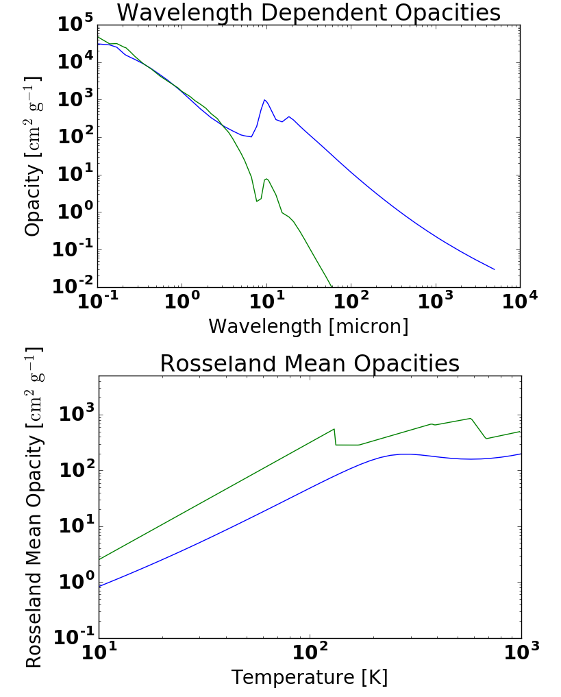
Figure 1.— The wavelength-dependent opacities from Preibisch et al. (1993), including the absorption (top, blue) and scattering (top, green) opacities, input into RADMC-3D. The calculated Rosseland mean opacities (bottom, blue) match the Rosseland mean of Bell et al. (1997). The piece-wise Rosseland Mean opacity based on D’Angelo et al. (2003) and implemented in the Pencil Code (bottom, green) only varies by at most a factor two from the calculation.

One of the novel aspects of our work is that, in addition to stellar illumination, the shock heating rate is used as extra heating rate input. This heating rate is given by

$$\mathcal{H}_{\rm sh}=\rho\nu_{\rm sh}\left({\bm{\nabla}}\cdot{\bm{u}}\right)^{2}.$$ (1)

where $\nu_{\rm sh}$ is an artificial shock viscosity, proportional to the positive part of ${\bm{\nabla}}\cdot{{\bm{u}}}$ according to

$$\nu_{\rm sh}=c_{\rm sh}\left<\max_{3}[(-{\bm{\nabla}}\cdot{\bm{u}})^{+}]\right>{\left[\min(\Delta x)\right]}^{2}{.}$$ (2)

Our treatment of shocks has been described in Haugen et al. (2004) and detailed in Paper I and Paper II. In Paper I we experimented with a range of values for the coefficient $c_{\rm sh}$, and found that it did not affect the result of the simulation as long as it is sufficient to smooth the shock into a resolvable length for the stencil (5 zones in each direction). When the shock is resolved the value of the shock viscosity coefficient does not change the amount of heating; rather, it only changes the volume (number of grid cells) over which the shock energy is spread. For the model shown in this work, we used $c_{\rm sh}=10$.

The shock heating rate is converted from code units into cgs units for use in RADMC-3D. The midplane and meridional resulting shock heating rates are shown in 2. As a result of testing done for the present work, the public version of RADMC-3D has been updated to include heated gas in every cell as a potential source of photons.

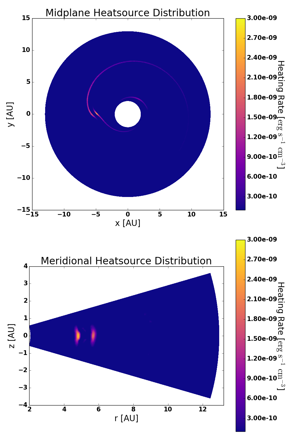
Figure 2.— The midplane (top) and meridional plane containing the planet (bottom), showing the shock heating rate distributions. Notice the spiral concentration of the shock heating rate in the midplane and the two lobes of shock heating on either side of the planet at 5.2 AU.

The star, made to match the T-Tauri star from Paper II, is placed at the origin. Its radius is 2 $R_{\odot}$, where $R_{\odot}$ is the solar radius; the star has effective temperature set to 4,000 K. HD 100546 is a Herbig Be star, so when deriving synthetic images we scale the distance to match the higher luminosity, as described in Sect. 3. A typical Monte Carlo radiative transfer simulation done for this work has $10^{7}$ photons. While more photons would yield greater resolution, the inclusion of an internal heating source, deep in the optically thick midplane, slows the radiative transfer computations considerably.

We note that the standard algorithm of Bjorkman & Wood (2001) assumes thermal equilibrium. This is not a valid approximation in the optically thick interior, where a Lagrangian fluid element is suddenly shock heated, then cools, but does not reach thermal equilibrium before being shocked again. The postprocessing approach nevertheless gives a better estimate of the temperature in the optically thin regions of the disk than done with the approximation used in the hydrodynamical model of Paper II.

3. Results and Discussion

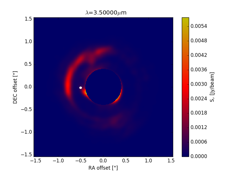
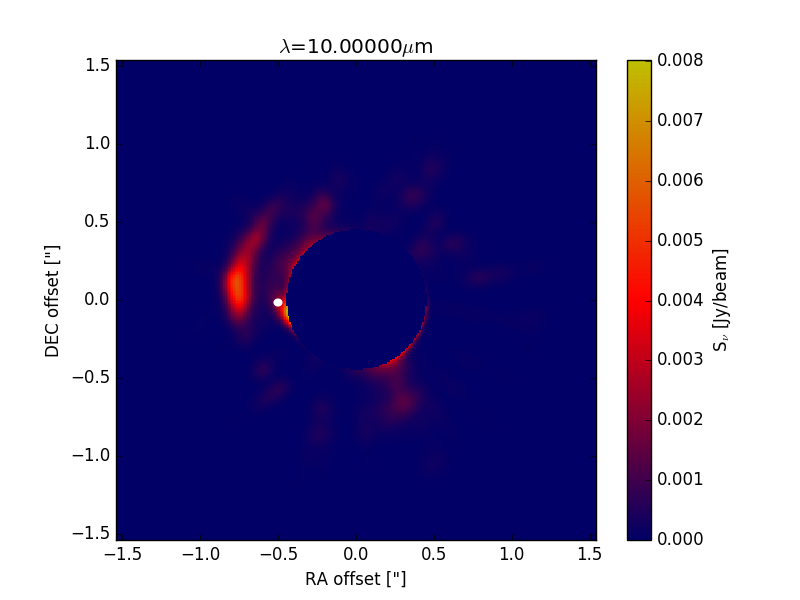
Figure 3.— Synthetic disk images with original heating rate and including scattering at wavelengths of 3.5$\mu$m (left) and 10$\mu$m (right). The white dots are the locations of the planet in the midplane. The coronographic mask size is 0.4” for the 3.5$\mu$m image and 0.45” for the 10$\mu$m image.

In order to compare our synthetic images to those of HD 100546 from Currie et al. (2014), both had to be on the same scale. Paper II assumed a T-Tauri star, so the disk temperature at 5 AU is of the same order of magnitude as that of a Herbig Be star’s disk a little inward from 50 AU; the factor 100 due to distance is mitigated by the factor $>$30 increase in luminosity. To match the relative sizes in the image, they are simulated as taken from a distance of 10 pc, compared to HD 100546 being 100 pc away (Berriman et al., 1994). This maps the position of 5 AU to the position of 50 AU in HD 100546 in arcseconds.

The images are given the same FWHM of 0.1”. A coronographic mask is applied, of radius 0.40”. This gives the mask a diameter of 0.80”, while the diameter of the mask in Currie et al. (2014) is approximately 0.70”. This small discrepancy can be accounted for by the uncertainty in the estimate of scaling the map from 5 AU to 50 AU. The images at 10 $\mu$m use a coronographic mask of radius 0.45”.

The face-on synthetic images at 3.5 and 10 $\mu$m are shown in 3. 4 shows the same images at 50^∘ inclination and 138^∘ position angle, the viewing perspective of HD 100546.

Currie et al. (2014) observed unexplained emission around HD 100546, which was not at the location of the planet HD 100546 b. It has been proposed that the emission is evidence for another planet, HD 100546 c (Currie et al., 2015). The images in 4 match in general morphology the observations of Currie et al. (2014). As evidenced in 3, the spiral feature in this case is not spiral in the sense of a feature that traverses different orbital radii, but in fact an arc at the same orbital radius, viewed at an oblique angle.

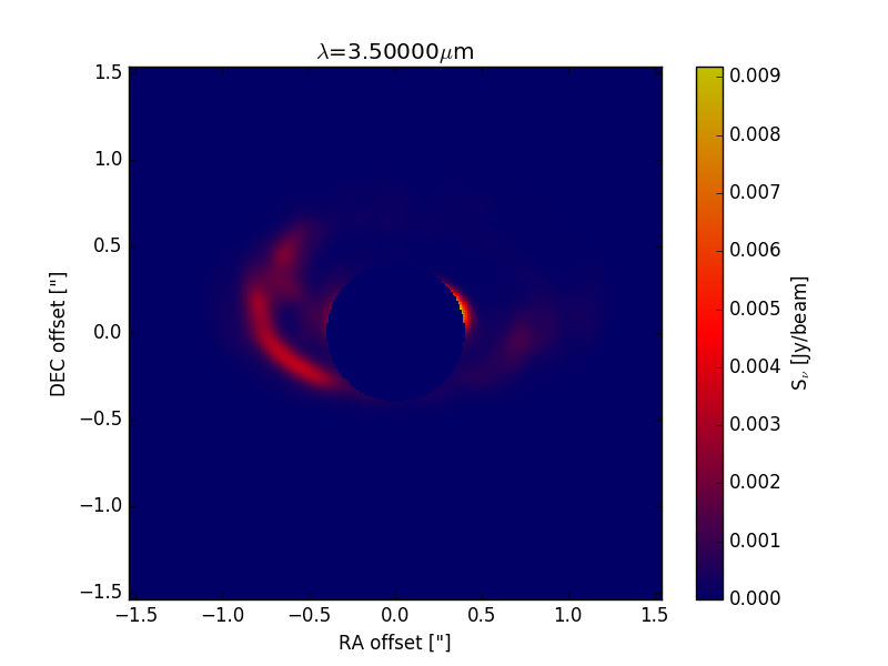
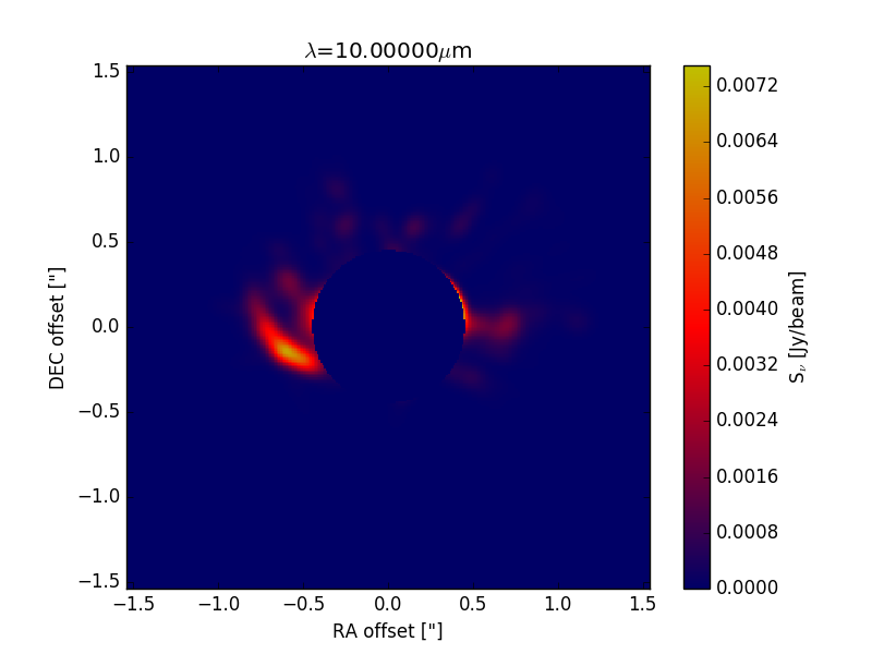
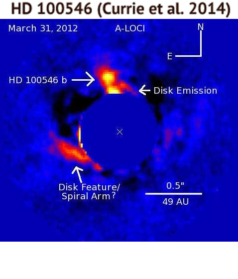
Figure 4.— Synthetic disk images with original heating rate and including scattered starlight at wavelengths of 3.5 $\mu$m (left) and 10 $\mu$m (center), with a 50^∘   inclination angle and a 138^∘  position angle. On the right is the $L^{\prime}$ band (3.4–4.1 $\mu$m) observation from Currie et al. (2014), with the same inclination and position angles. The location of the planet in the model is just behind the coronographic mask between 7 and 8 o’clock.

3.1. The effect of shocks alone

In order to isolate the emission coming from the planetary shocks, we calculate a set of synthetic images artificially removing the scattering opacity from the ray-tracing Monte Carlo simulation. These are shown in 5. The upper and lower images are calculated at 3.5 $\mu$m and 10 $\mu$m, respectively. The images on the left and right-hand side of the upper images have the shock heating rate artificially increased by a factor 10 and 20, respectively , while the lower images have the original shock heating rate, an increase by a factor of 10, and an increase by a factor of 20, respectively.

There is a distinct spiral feature in the infrared that appears more prominently when the shock heating rate is increased by larger factors. While the image with the original shock heating rate shows no signs of the spiral shock in the $L^{\prime}$ band, the Lindblad lobes are clearly defined with an increase in the shock heating rate by a factor of 10. At a factor of 20, both the Lindblad lobes and the spiral density wave generated by the planet are evident.

When modeled with the inclination and position angles of HD 100546, the synthetic observation (6, left) with a factor 20 increase to the heating rate does include a spiral feature that matches that of the observation. Images at longer wavelengths, from 8-15$\mu$m, show even clearer spirals with no increase to the shock heating rate. A synthetic image made at 10$\mu$m with the original shock heating rate but no scattering is shown at the same orientation as HD 100546 in 6, right panel. It is almost identical to the 10$\mu$m image that includes scattered light (4, center), meaning that the emission at 10$\mu$m is mostly thermal. The spiral feature shown in the left of the image again does match the morphology of the feature in the Currie et al. (2014) image.

The similarity in the thermal images suggests in principle that the source of the disk feature could be a high mass planet. However, this image is both much fainter than the scattered light image (note the intensity scale in each), and required an ad hoc factor of 20 increase of the shock heating rate to reproduce the $L^{\prime}$ observation.

4. Pinpointing the source of the emission

We explore in this section the origin of the emission in our models. Currie et al. (2014) finds that the emission feature in HD 100546 shows little polarization. This was taken as an indication that the emission must be thermal, and not scattered radiation. However, an error in the GPI pipeline made the feature seen in Currie et al. (2014) appear weakly polarized. In fact the emission should be interpreted as strongly polarized Millar-Blanchaer (2017, priv. comm.)

As we showed, a match in morphology with our 3.5 $\mu$m images requires an arbitrary increase in the magnitude of the shock heating rate of a factor 20, which may not be reasonable. Conversely, the spatial position of the intensity feature in our model (3) matches not the immediate vicinity of the planet, as expected if it came from the hot Lindblad lobes, but from the outer gap wall. Between 7 and 9 AU there is an increase in the disk scale height, puffing it upwards. It is this feature that produces the emission seen in 3 and 4. This outer gap reaches above the average disk height, and scatters photons from the central star towards the observer. 3 also shows that the contribution from shocks at 3.5 $\mu$m is negligible compared to the scattered light. Thus the emission in our model is not primarily thermal, but mostly polarized scattered light. On the other hand, at wavelengths of 10 $\mu$m or longer, thermal emission comes to dominate. In fact, a spiral feature matching the observation of HD 100546 is present in both the 10 $\mu$m image including scattered light (4, center) and including only thermal emission (6, right).

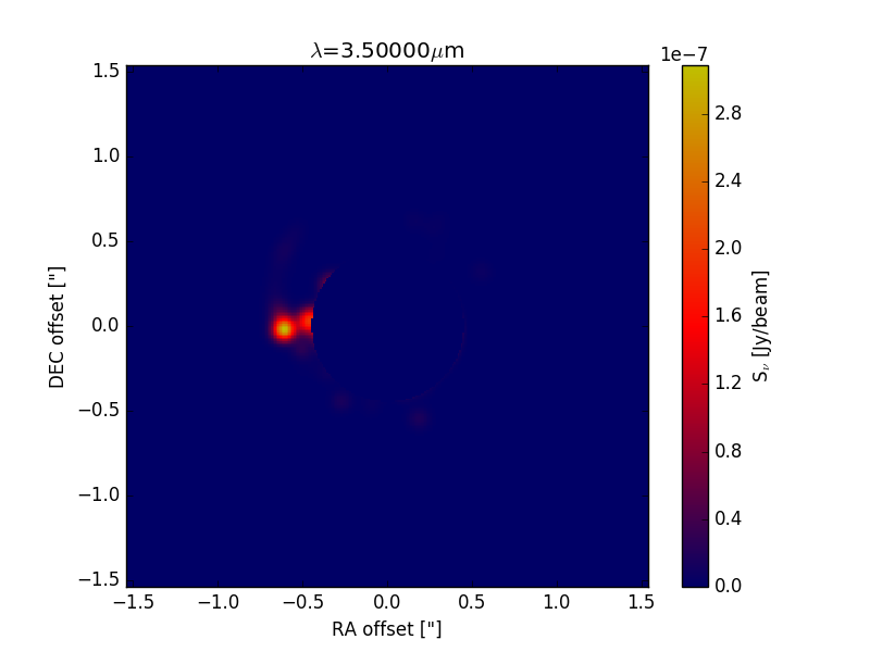
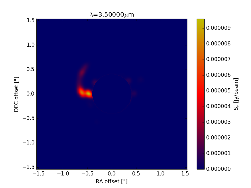
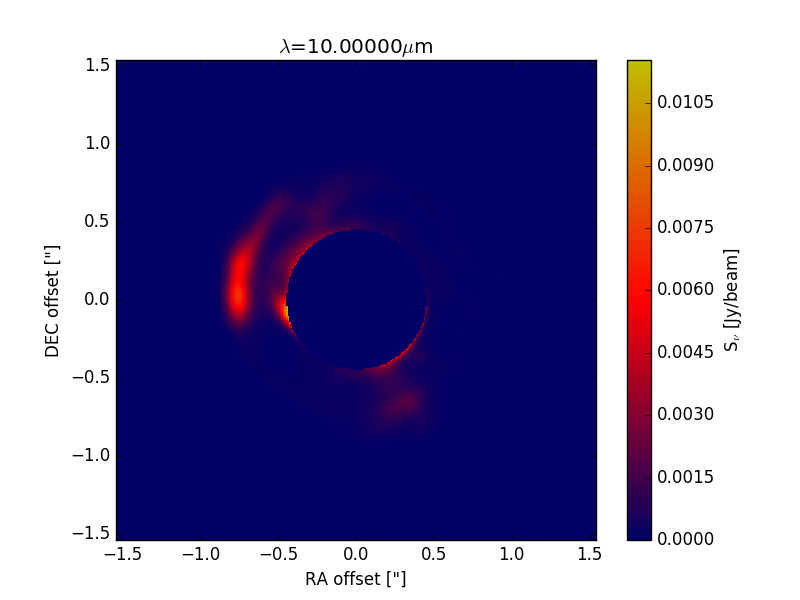
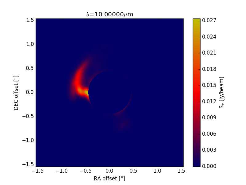
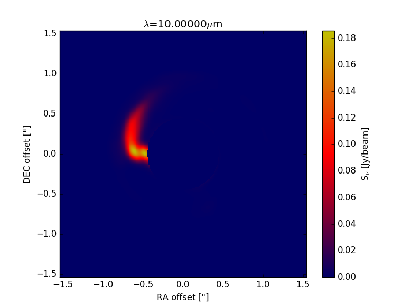
Figure 5.— Synthetic images generated by the ray-tracing function of RADMC-3D, neglecting scattering. Two high intensity regions are seen at a factor 10 increase in the shock heating rate (upper left) at a wavelength of 3.5 $\mu$m, while the primary spiral wave is seen at a factor 20 increase to the heating rate (upper right). At a wavelength of 10 $\mu$m, an arc is seen at an original heating rate (lower left), as well as more prominently when the heating rate is increased by a factor of 10 (lower center) and a factor of 20 (lower right). The images are made with 0^∘  inclination and position angles. Notice the difference in scale between these images and those of 3. The emission from shocks alone is orders of magnitude dimmer than the total emission in the 3.5 $\mu$m images. We conclude that scattering is the main source of emission at 3.5 $\mu$m.

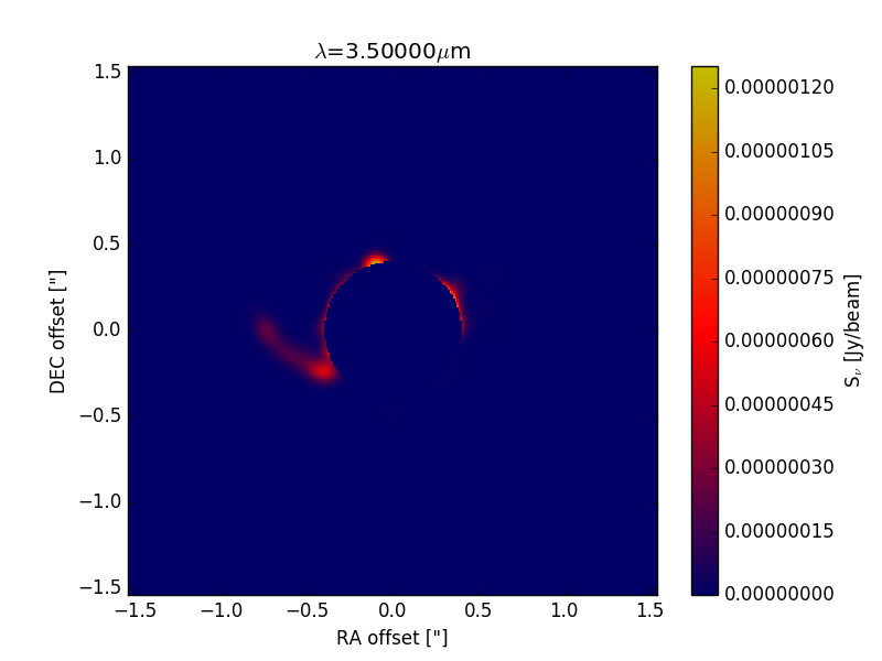
Figure 6.— Synthetic images without scattering with a 50^∘  inclination angle and 138^∘  position angle. The 3.5 $\mu$m image (left) was created with a factor 20 increase to its shock heating rate. The 10 $\mu$m image (right) was created using the original shock heating rate.

What determines the morphology of the scattered light image? We plot in 8 the normalized height of the $\tau=1$ surface $z/R$ (left panel), and the derivative of the height, $dz/dR$ (right panel). In the left panel the features with positive slope tilt toward the star and should appear in scattered light if they are not shadowed by features closer to the star, while features with negative slope should be shadowed. The highest feature at any given angle will appear in scattered light. Compare this image to the left plot of 3. With the right side of the image at 0^∘, increasing counter-clockwise, the region in the third quadrant between 270^∘ and 165^∘ in the outer disk is in the shadow of the inner disk. So is the region of the first and fourth quadrant between 75^∘ and 330^∘. In 3 we can see some of the inner disk scattering, but it is too close to the coronographic mask.

Figure 9, left panel, shows the same simulation as the left panel of 3, but with the coronographic mask reduced to 0.2”, and a logarithmic color bar. The inner spirals are bright, so the high areas behind them in the outer disk are in shadow. In the right panel of 9 we plot the radial location of the maximum normalized height at every angle. The surface it traces is a good match to 3.

Therefore, the match in morphology shown in the previous section between our synthetic image including scattered light and the image from Currie et al. (2014) can indeed be interpreted to show how a high-mass planet could produce an observational signature similar to that in the HD 100546 system.

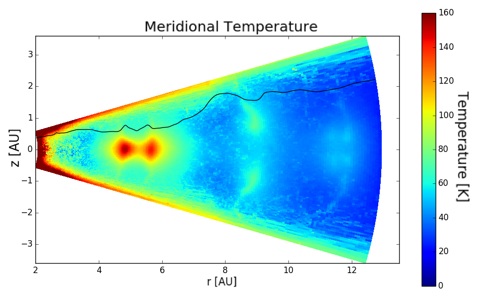
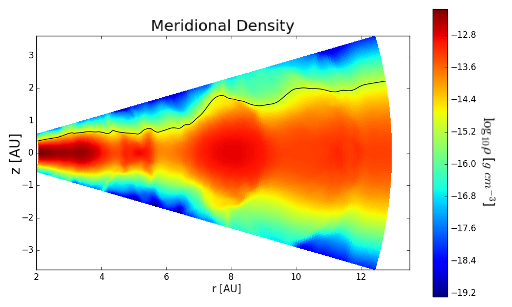
Figure 7.— Meridional temperature (left) and density (right) in the plane of the planet, with a contour drawn in black for the surface of $\tau=1$ at a wavelength of 3.5$\mu$m. This has no increase to the shock heating rate and is the result of a RADMC3D thermal Monte Carlo run with $10^{8}$ photons. The emission is not primarily from the thermal shocks but mostly from scattering off the outer gap wall between 7 and 9 AU that protrudes above the average disk scale height.

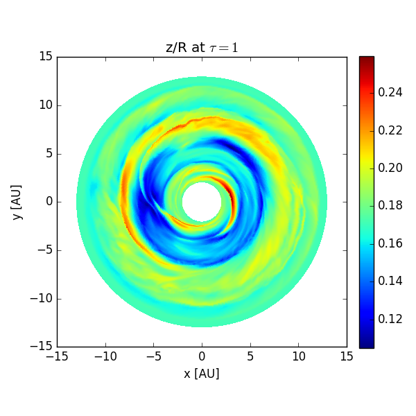
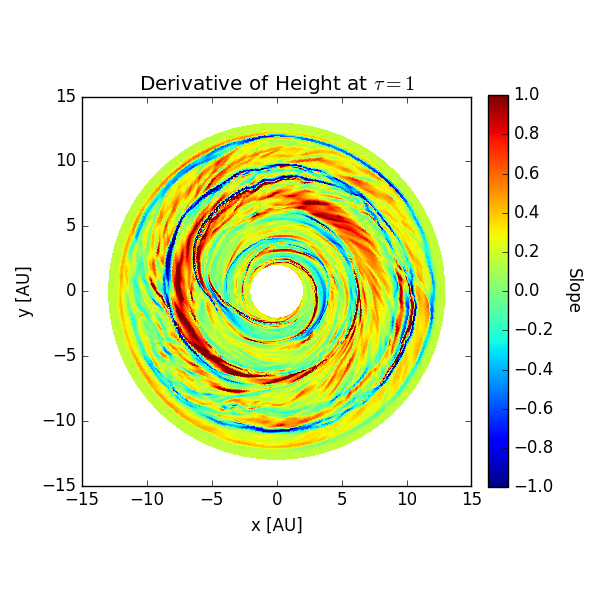
Figure 8.— Left. Normalized height $z/R$ at the surface of optical depth $\tau=1$. In this plot, the highest point at a given angle should be prominent in scattered light, while what is behind it should be shadowed. Right. The derivative of the height, $dz/dR$. Positive slopes tilt toward the star, while negative slopes tilt away, and thus are in shadow. Not all positive slopes should appear in scattering, because some may be shadowed by features further in.

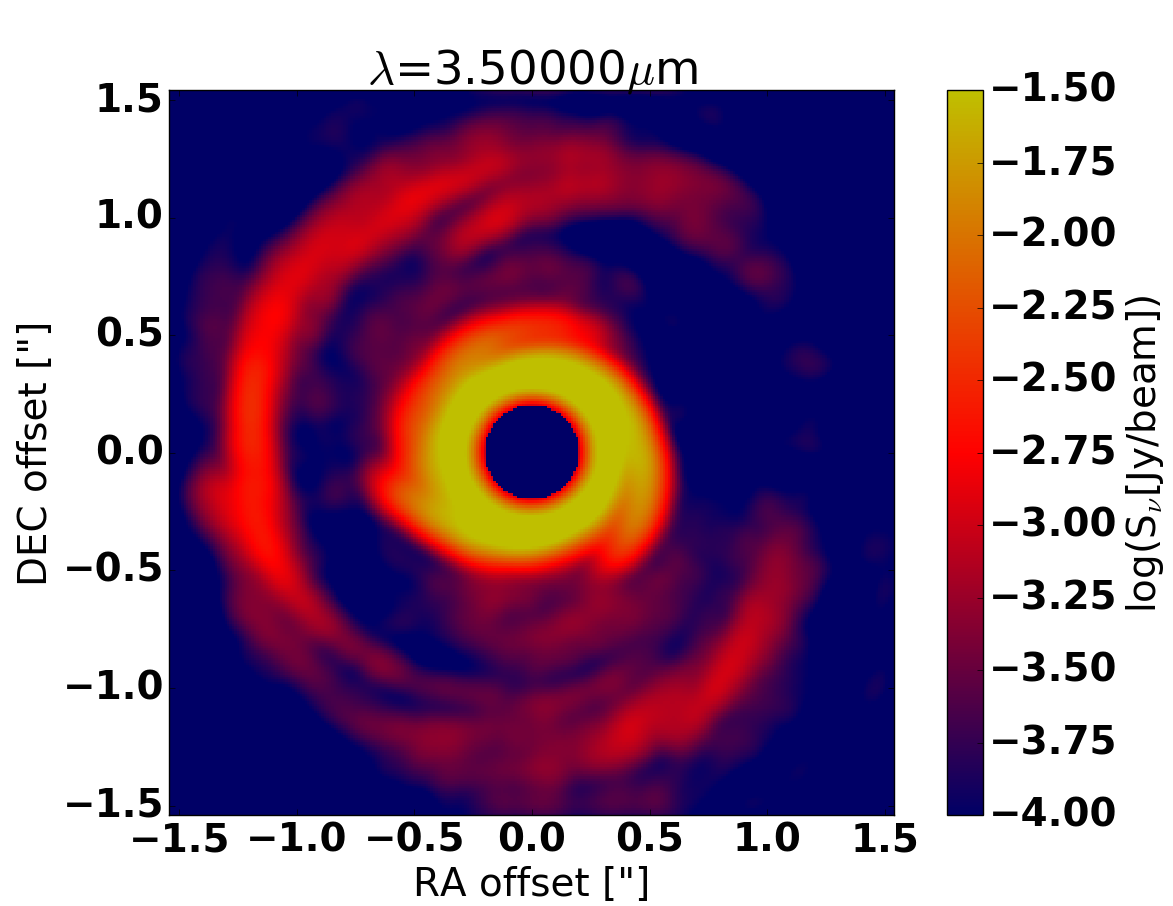
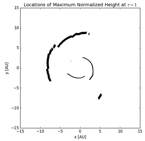
Figure 9.— Left. Same as the left panel of 3, but with a smaller coronographic mask (0.2”), showing the inner spirals, and plotted in logarithm. The inner spirals seen in 8 shadow the outer disk. Right. The radial location of the maximum normalized height at a given angle. The surface it traces matches the prominent emission features in 3.

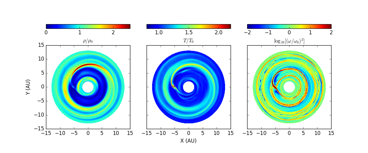
Figure 10.— State of the disk midplane: density (left), temperature (middle), and vorticity (right). The density shows a feature in the outer edge of the gap, with peak density between 8 and 9 o’clock. The temperature plot shows that the outer gap edge is hotter than the gas around it. The vorticity does not particularly show a strong vortex, although the density maximum stands on a vorticity depression.

4.1. Ruling out a vortex

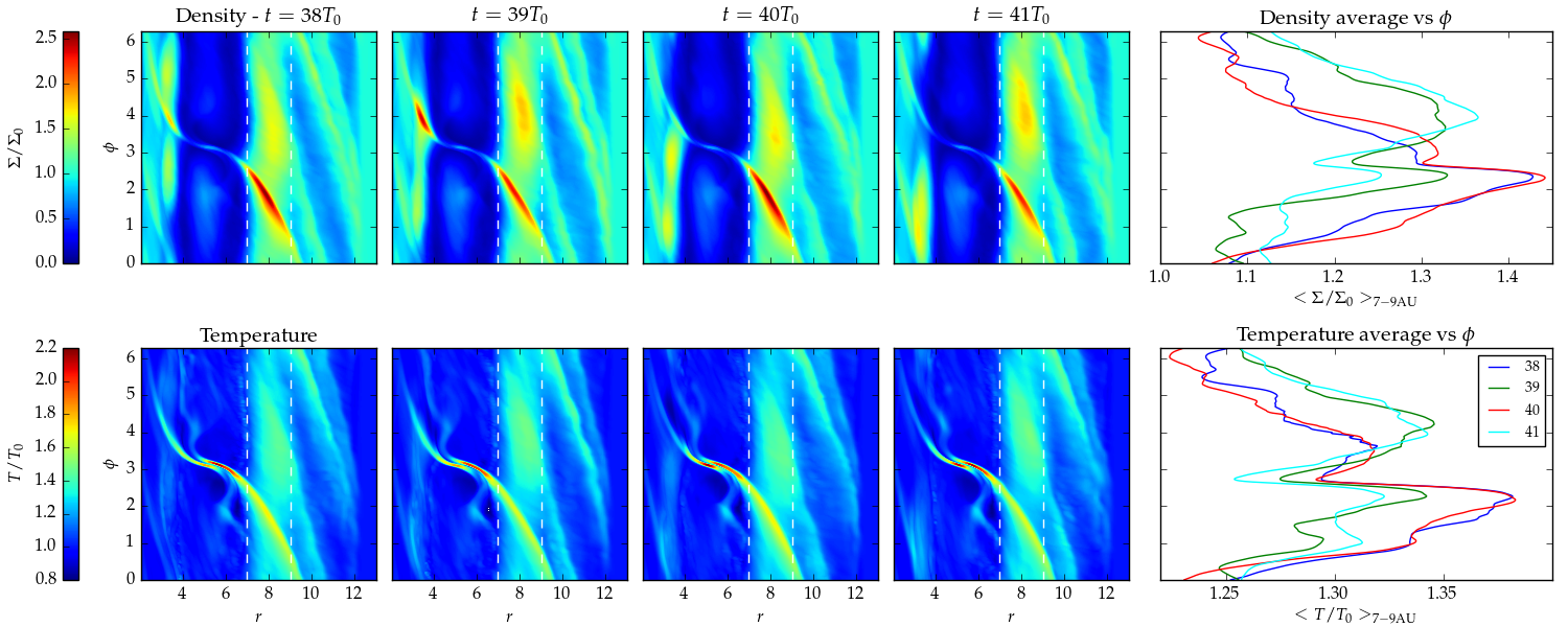
Figure 11.— Density (upper plots) and temperature (lower plots) at the midplane in four snapshot s separated by one planetary orbit. The rightmost plot shows the average in the region between 7 and 9 AU as a function of azimuth. We see that the high density feature is stationary with respect to the planet. A vortex is an independent entity and would show synodic motion, so we rule out the vortex possibility. However, the radial averages show periodic variation at the synodic period (2 planetary orbits), at the 10% level. We conclude that even though a vortex may be present, the corotating feature is dominant. The maxima of density and temperature in the second quadrant is due to the presence of the primary spiral arms launched at Lindblad resonances.

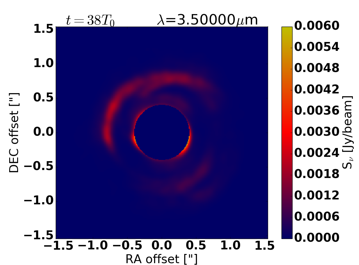
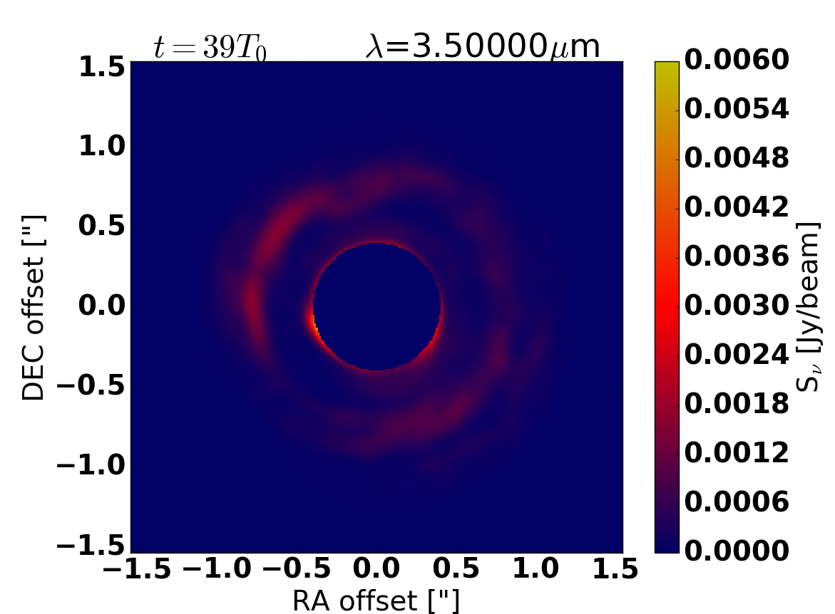
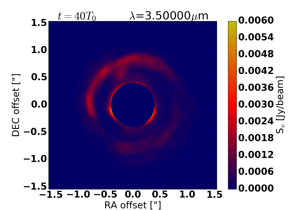
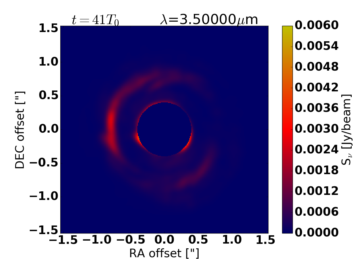
Figure 12.— Scattering image in the same snapshots as 11. The intensity maxima occur outside the gap and mostly in the second quadrant. The high density features in the snapshots are mostly located in the third quadrant, so they are not responsible for the emission.

The bright feature in the second quadrant is seen in scattered light, not thermal emission, and results from an enhanced scale height immediately outward of the planet. The enhancement is asymmetric, lifting the side next to the planet more than the side opposite to it.

One type of hydrodynamical feature that produces asymmetry in disks is a vortex (Lyra & Lin, 2013; van der Marel et al., 2013), which is expected to form at planetary gap edges as a result of the Rossby wave instability (Lovelace et al., 1999; de Val-Borro et al., 2006; Lyra et al., 2009). We plot in 10 the midplane values of density, temperature, and vorticity. The temperature is that calculated in the original Pencil Code simulation, not the MC computation. There is a noticeable density increase and temperature increase associated with the location of the bright feature, next to the planet. There is an enhancement in density at the outer gap wall, near opposition, between 8 and 9 o’clock, which could be a vortex. The whole outer gap wall is a vorticity depression (10, right panel), as expected, but a clear localized vorticity minimum is not associated with the density maximum.

To see if there is a correlation between the high density feature and the scattering images, we plot in 11 four snapshots of the disk, from 38 to 41 orbits of the planet, spaced one orbit apart. The upper panels show the density, the lower panels the temperature. The rightmost plots show the density and temperature as a function of azimuth, averaged in the region from 7 to 9 AU, bracketed by the dashed lines in the contour plots. The high density feature is at $\phi\approx 4$.

For comparison, we plot the intensity calculated from the respective snapshots, shown in 12. The planet is at $\phi=\pi$ (at nine o’clock), and azimuth increases counterclockwise. In the panels of 11 the feature is located in the third quadrant. In the intensity plots of 12 the maxima are located in the second quadrant mostly. The locations do not match, so we must seek another explanation.

More intriguingly, notice that the high density feature seems stationary in the reference frame of the planet. An independent feature at 8 AU is close to the 2:1 resonance with a planet at 5 AU, and thus should alternate conjunction and opposition with the planet in snapshots separated by one planetary orbit. The fact that this does not happen for this feature is clear indication this is not an independent feature, so we rule out the vortex possibility. Yet, notice that the right plots of 11 clearly show variation at the 10% level with a period of two orbits, the synodic period. We conclude that the outer gap edge harbors underlying independent structures, but they are of lower prominence compared to the overarching stationary pattern.

4.2. Secondary Spiral

The fact that the feature, both in the midplane (11) and in the intensity plots (12), seems to corotate with the planet brings us to consider the spiral patterns again. While the primary arm is launched at Lindblad resonances, Juhász et al. (2015) and Zhu et al. (2015) call attention to the existence of secondary spiral features, which Fung & Dong (2015) and Lee (2016) show are launched at the 2:1 resonance (similarly, tertiary arms are also present, launched from the 3:1 resonance, and so on). These secondary arms for high-mass planets were already noticed by de Val-Borro et al. (2006), but their origin or nature had not been studied. Fung & Dong (2015) and Dong et al. (2016) explored their observational properties, finding that they are prominent in scattered light, and also derive a relationship between the planet mass and the angular distance between the primary and secondary arms. For a 5$M_{J}$ planet, they should be separated by $\approx$141^∘.

We plot in 14 snapshots of the disk midplane, with one planetary orbit cadence. The secondary arm in the inner disk is visible from the second orbit, and in the outer disk from the fifth or sixth orbit. A labeled closeup of the features in the last snapshot can be seen in 13. The outer spiral is seen as a density enhancement between the primary spiral and its periodic continuation, launched from $r\approx 8$ AU and $\phi$ between $\sim$5–6.

The high density feature seen in 11 is obvious in later snapshots and clearly had its origin in the secondary outer arm. The panel in the lower right is an average of all snapshots. The measured separation is $\approx$150^∘, within 6% of the value predicted by the formula of Fung & Dong (2015). We conclude that indeed we are seeing the secondary spiral.

A novel aspect of our model is that we also calculate the temperature, showing that the outer gap edge and the secondary spiral are hotter features. Being so, they raise the scale height locally and increase the intensity in the scattered starlight synthetic images. The spiral is a stationary feature in reference to the planet, which matches the stationary area of high intensity seen in 12. Another difference between our model and those of Fung & Dong (2015) and Dong et al. (2016) is that we do not use an artificial eddy viscosity. The large scales of the flow are effectively inviscid. Either the lack of viscosity or the presence of buoyancy, or both, can lead to the discrepancies between the fuzzy spirals we see versus their well-defined ones.

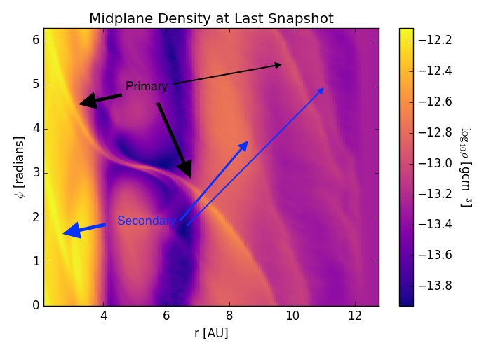
Figure 13.— Density at last snapshot, in polar coordinates, showing the primary spiral, launched at the Lindblad resonances, and the secondary spiral. The thinner arrows show the periodic continuation of each.

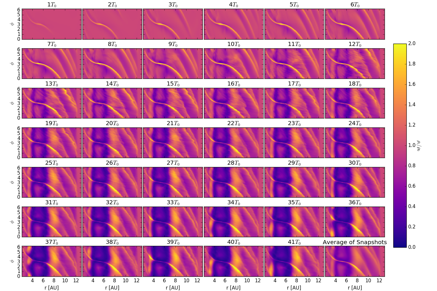
Figure 14.— Density in the midplane in snapshots from one to 41 orbits, with one orbit cadence. In addition to the primary Lindblad spiral, the planet launches secondary spiral arms from the 2:1 resonance, located at $\approx$ 3 and 8 AU. The inner secondary is seen already at the second snapshot. The outer secondary spiral is visible from the fourth snapshot but more prominently at the sixth. It is seen as an enhancement in density radially inwards from the rarefaction wave of the primary spiral, launched from $r\approx 8$ AU and $\phi\approx 5$. The secondary spirals overlap with the forming planetary gap edges as time increases.

4.2.1 Eccentricity

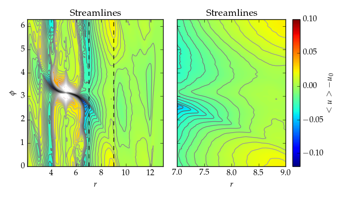
Figure 15.— Flow streamlines. The color code refers to the midplane speed, $\sqrt{u_{r}^{2}+u_{\phi}^{2}}$, normalized by the initial value of this quantity. The right plot zooms in at the region between 7 and 9 AU. One sees that the flow is slower at opposition and faster at conjunction, as would be expected if the orbits were slightly eccentric, with aphelion occurring at opposition.

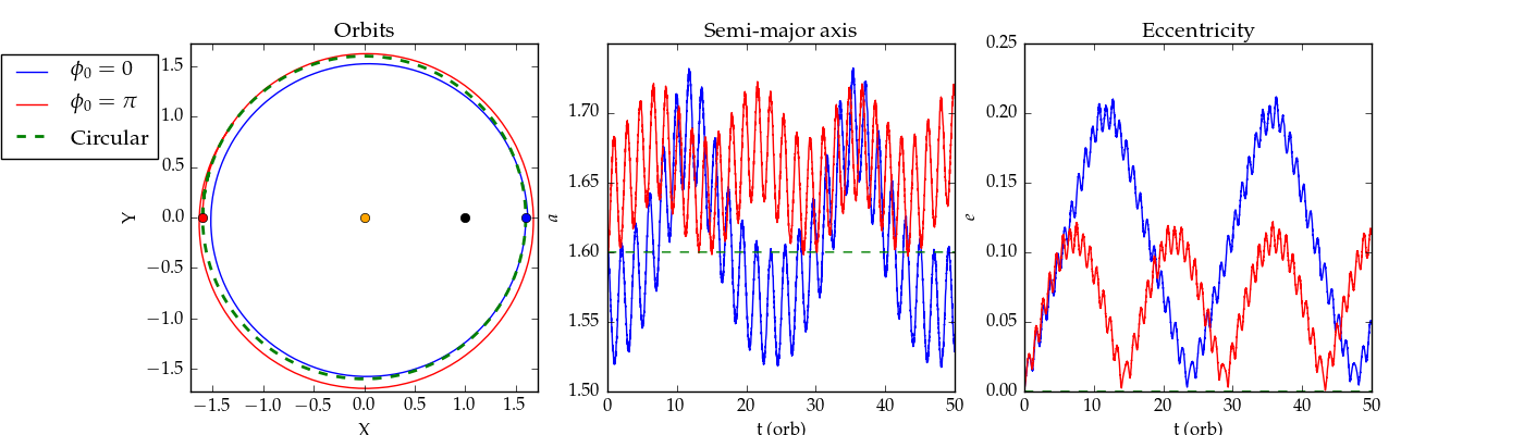
Figure 16.— We place two test particles in the same outer orbit, initially circular, but with the particles started at opposition (blue dot) and at conjunction (red dot). An orange dot and a black dot mark the position of the fixed star and planet, respectively. A circular orbit (green) is shown for comparison. The first two orbits are shown in the leftmost plot (blue and red lines). The particles develop an eccentricity, both having closest approach to the planet (at $\phi=0$) in aphelion. The middle panel shows the semi-major axis and the right panel the eccentricity. The particle at opposition is more heavily perturbed by the planet. Both orbits should change in time as a result of the perturbation.

Although we identify the secondary spiral as the culprit of the lopsided emission we see in our models, we have to examine as well to what degree eccentricity excitation is or is not influencing the results. Kley & Dirksen (2006) argue that a massive planet turns the disk gap eccentric by removing gas from the 2:1 resonance. This resonance provides eccentricity damping so, without it, the gap walls exponentially grow into an eccentric state within some hundreds of years. The timescale for eccentricity pumping, for a 5$M_{J}$ planet is 250 orbits, reaching a saturation value of 0.25 in $\approx$700 orbits.

We assess to what eccentricity our system has grown, if any. If a system of e-folding time $\tau=250T_{0}$ saturates at $e_{\rm sat}=0.25$ at $t_{f}\approx 700T_{0}$, then at $t=40T_{0}$ it should have grown to only

$${\color[rgb]{0.0,0.0,0.0}e} {\color[rgb]{0.0,0.0,0.0}=} {\color[rgb]{0.0,0.0,0.0}e_{\rm sat}\exp\left[-\left(t_{f}-t\right)/\tau\right]}$$ (3)

$$= 0.25\exp\left[-\left(700-40\right)/250\right]\approx 0.02$$

We plot in 15 the streamlines of the flow in the midplane. The color code refers to the reference speed $(u_{r}^{2}+u_{\phi}^{2})^{1/2}$ normalized by the initial condition. The average is in time, from 20 to 41 orbits, one snapshot per orbit. The right panel zooms in the region from 7 to 9 AU, between the dashed lines. It is seen that the azimuthal range next to the planet has a slower flow than the azimuthal range opposite to the planet. Obeying the continuity equation, the slower gas has to get denser, and the faster gas thins. This situation is consistent with the density plots.

To understand how a situation like 15 can arise, we perform a test placing massless particles at conjunction and at opposition with a 5$M_{J}$ planet; the results are shown in 16. The star is at the center (orange dot in the left panel) and the planet at $r=1$ (black dot in the left panel). We place the particles initially at $r$=1.6, close but not exactly at the 2:1 resonance. The left panel shows two orbits of integration. The first particle begins initially at opposition (at $\phi=0$, blue dot). As the run starts, its orbit becomes eccentric; at closest approach to the planet it reaches aphelion (blue line). A circular orbit is shown as a dashed green line for comparison. The second particle begins at the same radial position but initially at conjunction (at $\phi=\pi$, red dot). Its orbital eccentricity also grows, and at closest approach to the planet it also reaches aphelion, but at a slightly larger semimajor axis (red line). Eccentricity and the semi-major axis do not remain constant (middle and right panel of 15), starting at eccentricity $e<$0.05 and later growing to as much as $e=0.1$ for the outer and $e=0.2$ for the inner particle. There is orbital variation, especially in the case of the inner particle, due to the strong perturbation of the planet. This precession will change on relatively longer timescales the argument of aphelion, and with that the azimuthal location of the intensity maximum. We caution also that the pressure field may change this picture.

Since the encounter with the planet occurs at aphelion and in this region the motion is slower, we can expect the density there to be higher. Taking the particle trajectories as a proxy for streamlines, it seems that this eccentricity, caused by the massive planet deforming the streamlines, can also lead to a lopsided azimuthal overdensity. Although the eccentricity in our simulation is small, the saturation eccentricity of 0.25 predicted by Kley & Dirksen (2006) is far from negligible. The hydrodynamic model will need to be run for far more than the current 40 orbits in order for the eccentricity to saturate and more accurate observational predictions of the outer gap edge to be made.

4.3. Image catalog

We finish this work by presenting in the Appendix a catalog of images generated from our simulations with shock heating, that may serve as a guide for interpreting future observations.

5. Conclusions

We have for the first time derived synthetic images including the heating produced by the shocks that high-mass planets cause in their parent disks. During this work, the public version of the code RADMC-3D was modified to include a general heating rate leading to emission from every cell.

We explore the observational signatures of this shock heating, using the hydrodynamical model of Paper II of an embedded 5$M_{J}$ planet, where the planetary shocks were first characterized in three dimensions. We perform post-processing radiative transfer simulations on this hydrodynamic model, finding that planetary shocks are able to match the general morphology of the thermal emission in the observations of HD 100546 from Currie et al. (2014). Yet, synthetic images in the $L^{\prime}$ band generated by this post-processing technique were able to match the observed morphology only if an ad hoc factor 20 increase to the shock heating rate is considered. At longer wavelengths (10 $\mu$m), no ad hoc increase is needed as the observational signature is prominent. We predict that at wavelengths of 10 $\mu$m or longer, the emission will come to be dominated by unpolarized thermal emission rather than polarized scattered emission.

We find that the best match to the observed feature in the $L^{\prime}$ band comes not from thermal radiation from the shock, but from scattered starlight off the outer edge of the planetary gap. The gas immediately outward of the planetary gap shows a raised scale height, with the surface of $\tau=1$ matching primarily density, not temperature, contours, and lifted above the average height of the disk atmosphere. Moreover, the density enhancement is lopsided, with the side next to the planet being denser and more prominent in the synthetic image than the side opposite to the planet. The fact that scattering provides such a good match to the observed features can be taken to imply that the emission in HD 100456 as seen in Currie et al. (2014) is not thermal.

In tracing the origin of the azimuthal asymmetry in the disk intensity outside the gap, we see that in the midplane the side next to the planet is indeed denser and hotter than the opposite side. The maximum density in the $\tau=1$ surface coincides with what looks at first as the eye of a vortex. Yet, inspecting other snapshots, the feature’s location does not always match the intensity maximum; moreover, the feature is stationary in the reference frame of the planet, which led us to identify it with a secondary spiral arm, excited at the 2:1 resonance. The cause of the asymmetry is ultimately the presence of this secondary spiral arm intersecting with the disk gap outer edge. It increases the density and temperature in the region, thus raising the height of the $\tau=1$ surface there.

If the outer gap edge is so prominent in thermodynamically evolving disks with high-mass planets, we expect that eccentricity, if present, should have a significant observational signature. Measuring the streamlines we find that the gas is faster in the opposite side and slower next to the planet, as would be expected if the orbits were eccentric, with aphelion on the planet side. Placing two test particles in orbit, initially in circular Keplerian orbits, one starting in opposition and the other exterior conjunction, we see that, perturbed by the planet, both quickly develop orbits with different semimajor axes, but closest approach to the planet in aphelion. Due to the strong perturbation of the planet, the orbits evolve in time, and we do not always expect the planet to be aligned with the orbital apsides. The eccentricity is in fact just starting to develop after 40 orbits. It will require simulating the system for longer times to determine the effect of a saturated eccentricity, which we defer to a future study.

Future research to confirm the conclusions presented should vary the distance to the planet in the hydrodynamic model, run the radiative transfer around a different type of star to match specific observations, and change the smoothing of planet mass. These studies would be individual to certain observations of spiral emissions and should be tailored to each system. Measurements of polarization at wavelengths longer than 10 $\mu$m will reveal if thermal emission from the shock can indeed be detected.

We present here a catalog of images generated from our simulations with shock heating, that may serve as a guide to future observations.

In 17 we show images calculated at 3.5 $\mu$m, with scattering included. From top to bottom the position angles are 0^∘, 90^∘, 180^∘, and 270^∘. From left to right the images are shown in inclination angles of 0^∘, 45^∘, and 80^∘.

In 18 we show images in the same orientations as 17, but at 10 $\mu$m and with the original heating rate. In Figs 19 and 20 we show the same images but with scattering excluded, i.e., only the effect of shocks.

Comparison between 17 and 19 shows that scattering is by far the main feature in this waveband. The luminosity from the shocks, faint and deep within the midplane, is orders of magnitude smaller than the scattering off the disk surface.

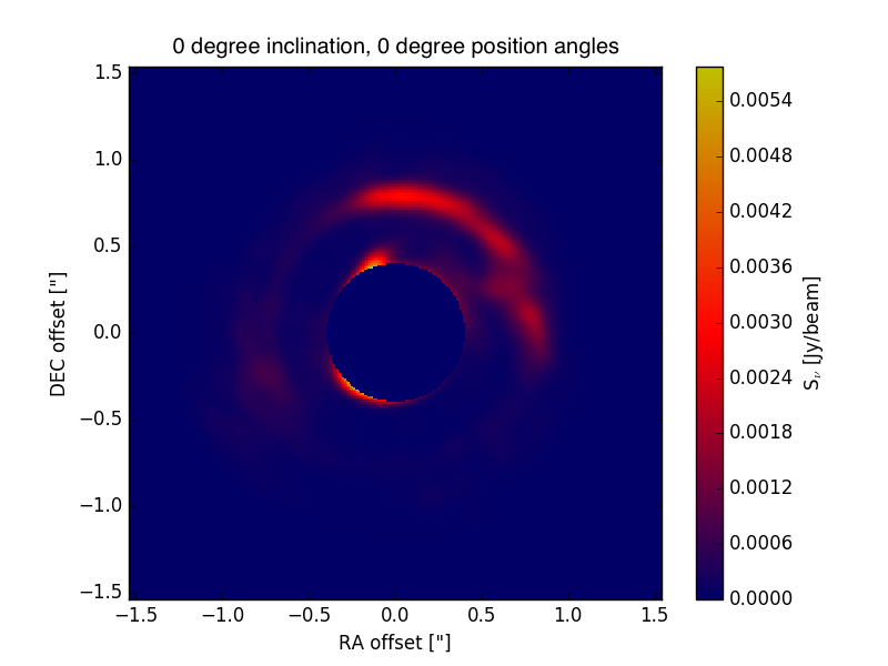
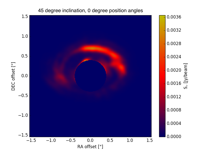
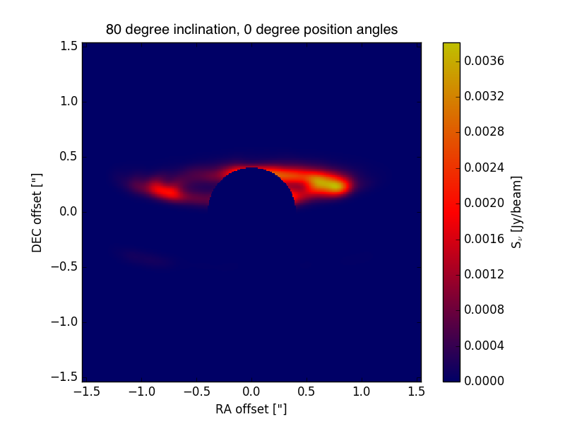
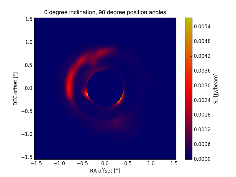
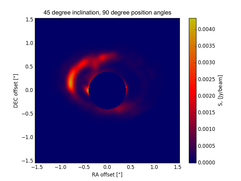
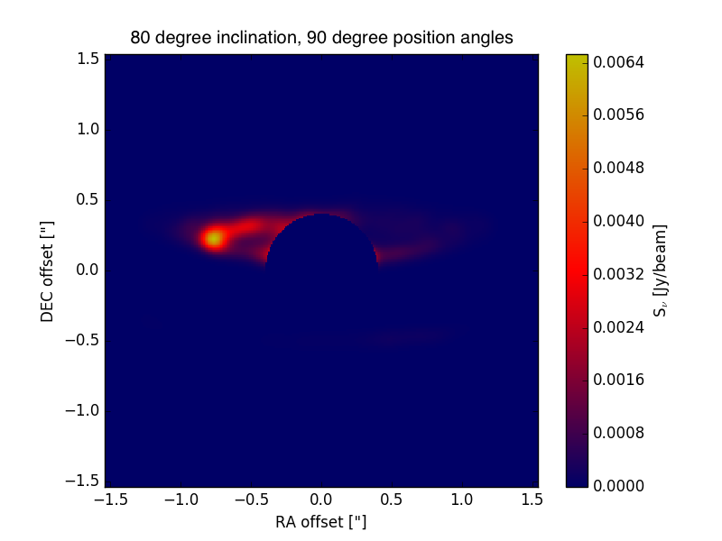
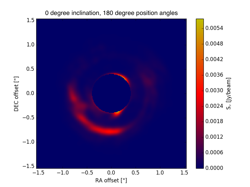
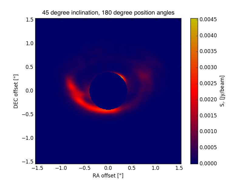
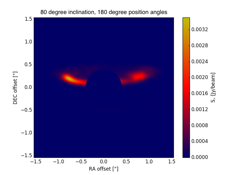
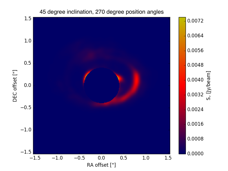
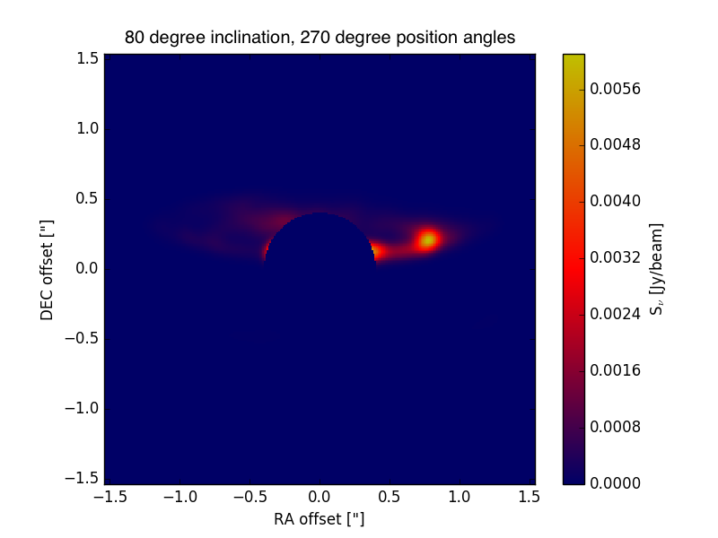
Figure 17.— Array of synthetic images at 3.5 $\mu$m with scattering included. The original shock heating rate is used. Rows from top to bottom are position angles of 0^∘, 90^∘, 180^∘, and 270^∘. From left to right are inclination angles of 0^∘, 45^∘, and 80^∘.

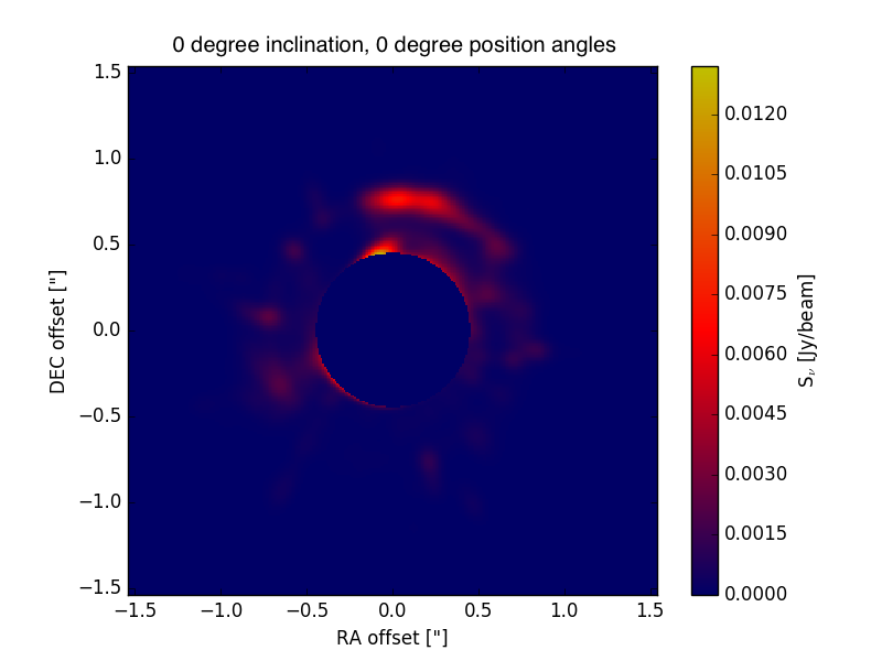
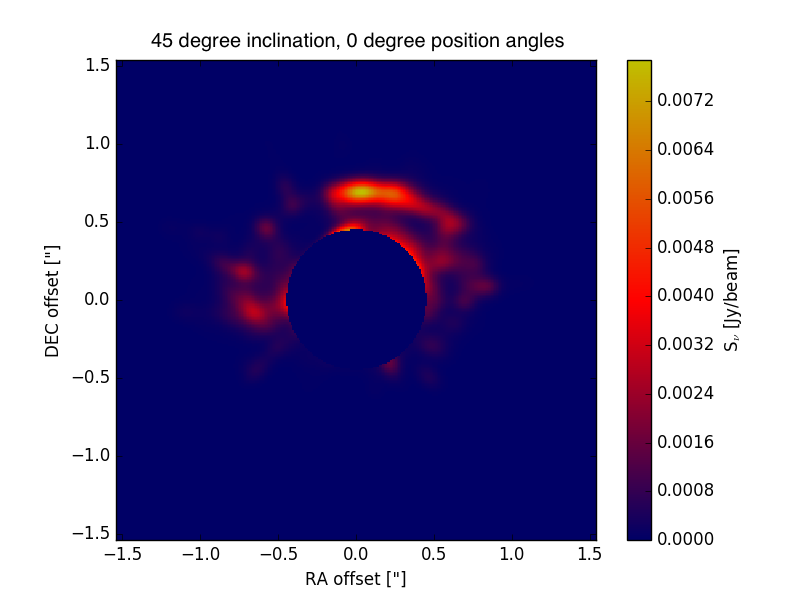
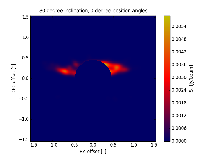
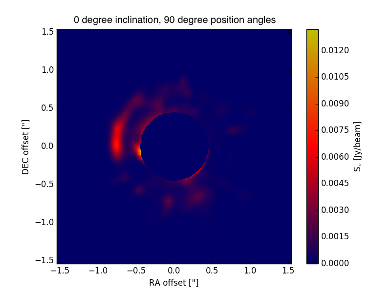
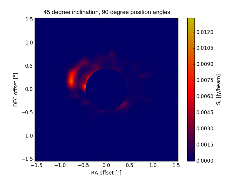
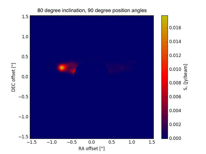
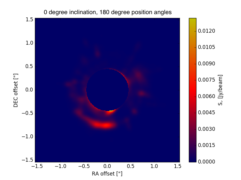
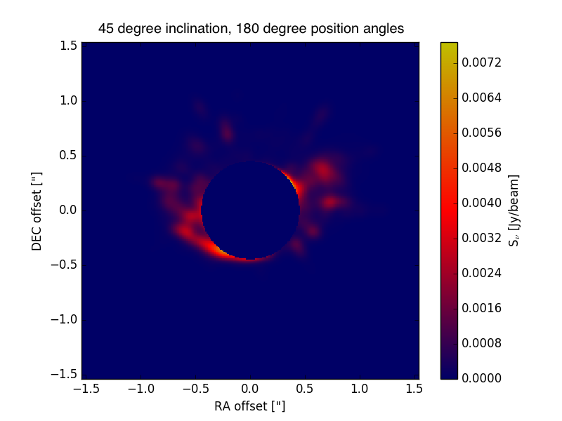
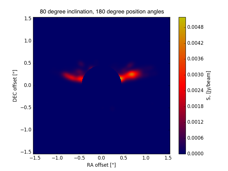
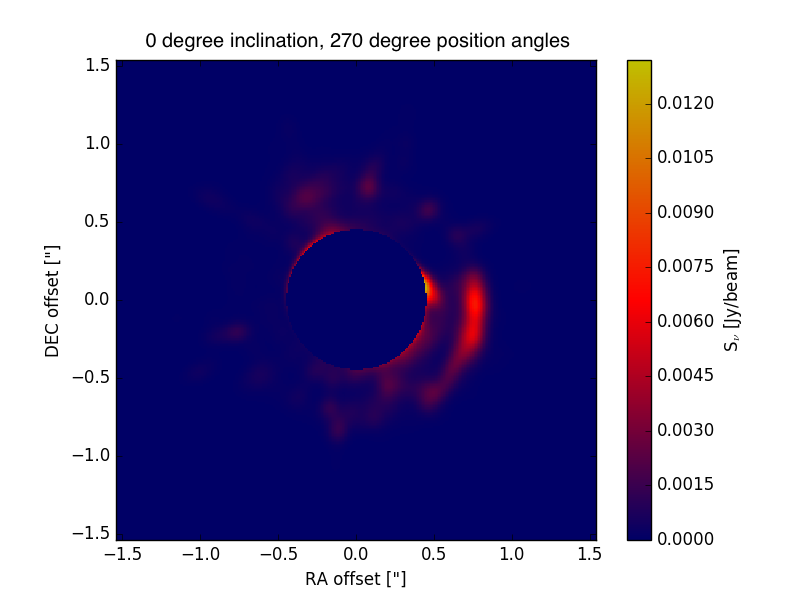
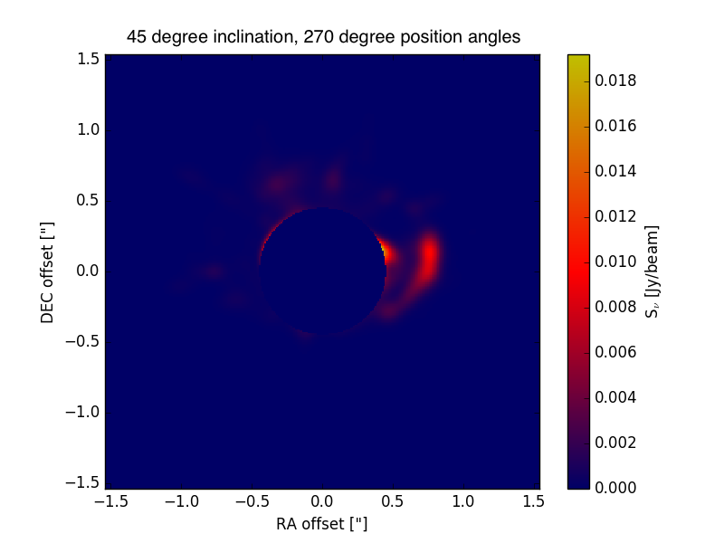
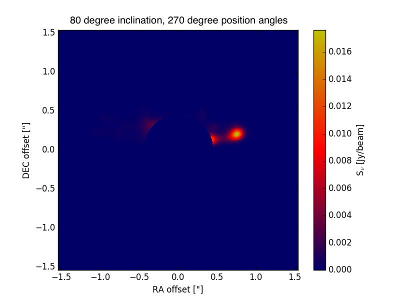
Figure 18.— Array of synthetic images at 10 $\mu$m with scattering included. The original shock heating rate is used. Rows from top to bottom are position angles of 0^∘, 90^∘, 180^∘, and 270^∘. From left to right are inclination angles of 0^∘, 45^∘, and 80^∘.

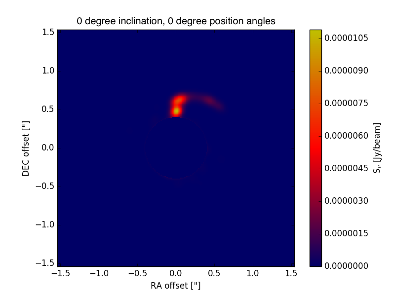
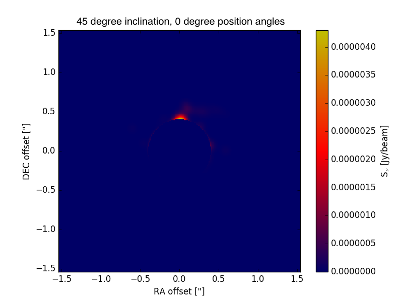
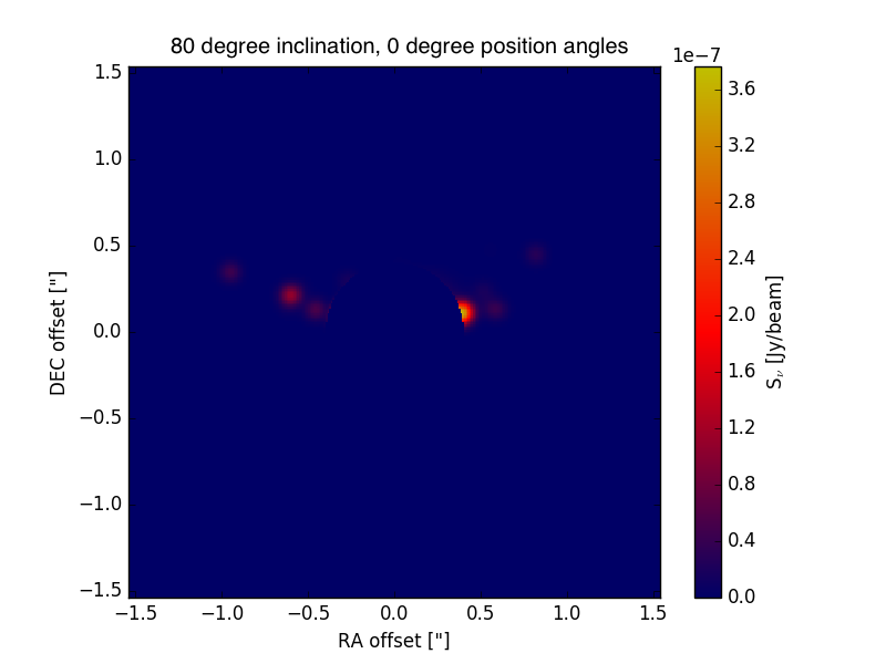
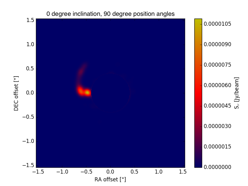
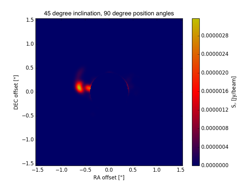
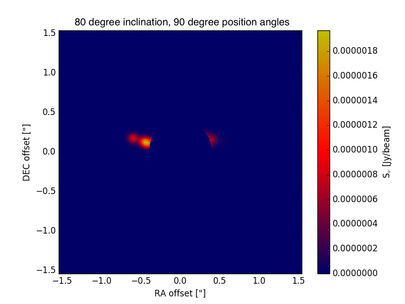
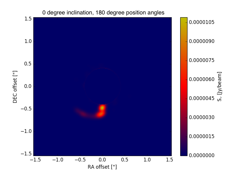
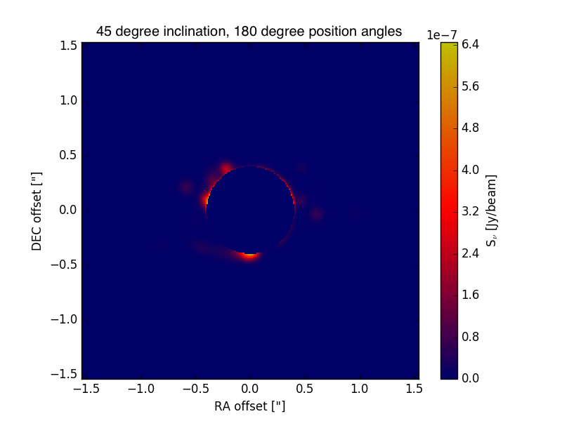
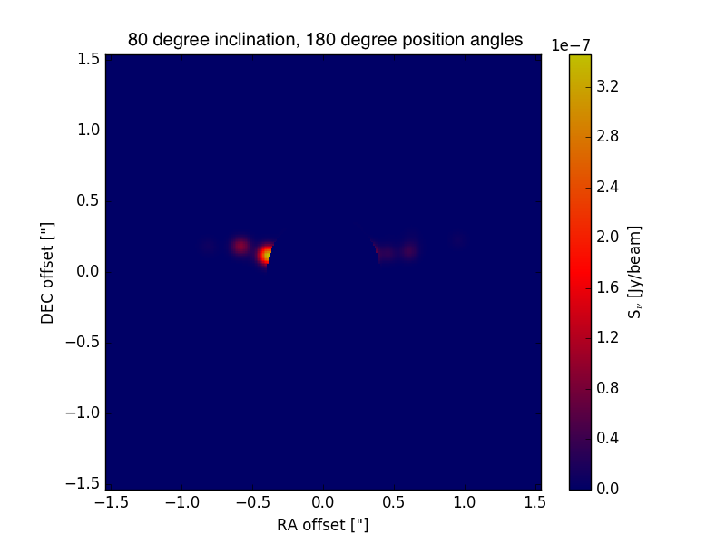
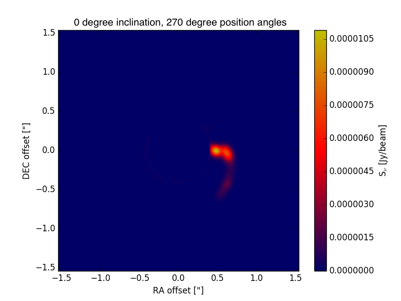
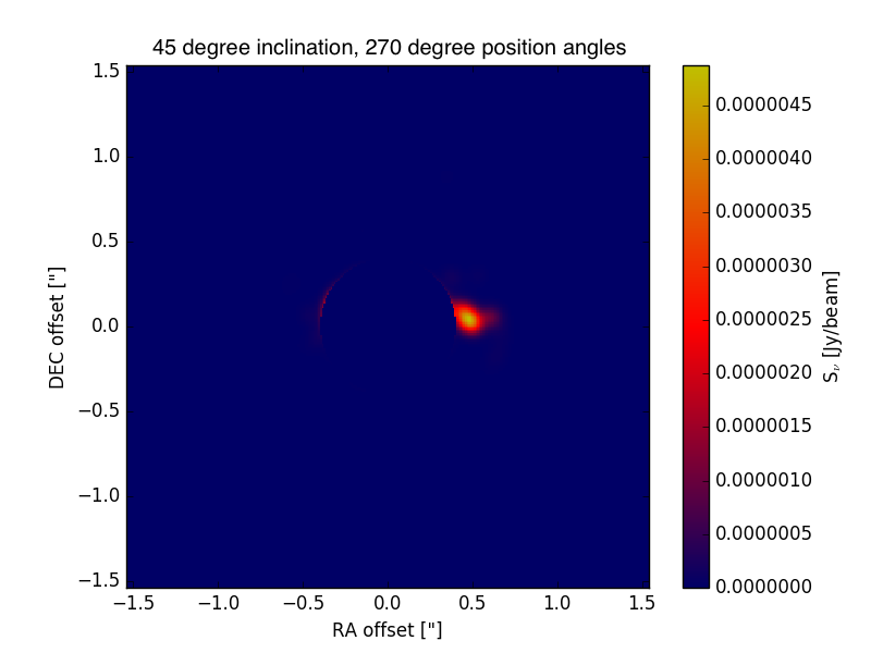
Figure 19.— Array of synthetic images at 3.5 $\mu$m without scattering included. The shock heating rate is increased by a factor 20, since images produced with the original shock heating rate show no distinguishable features. Rows from top to bottom are position angles of 0^∘, 90^∘, 180^∘, and 270^∘. From left to right are inclination angles of 0^∘, 45^∘, and 80^∘.

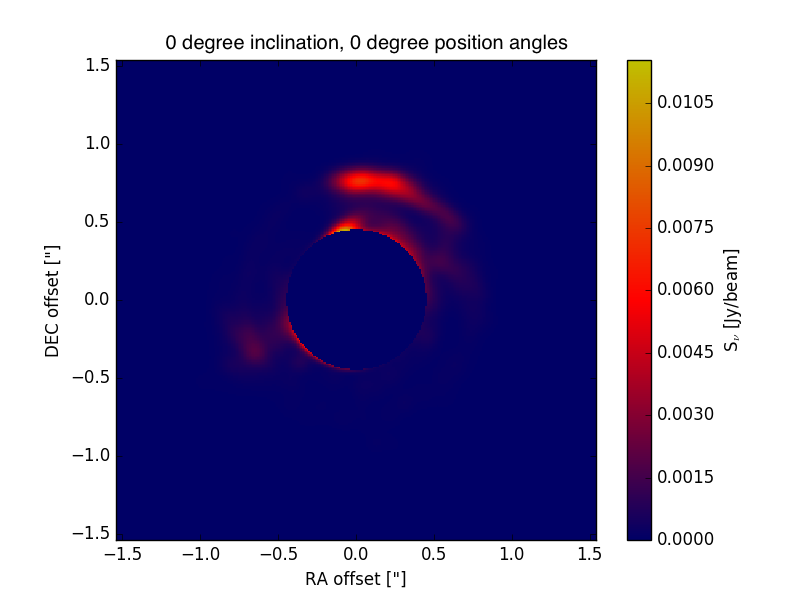
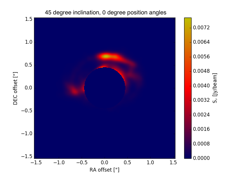
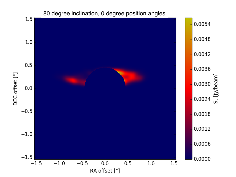
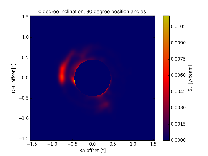
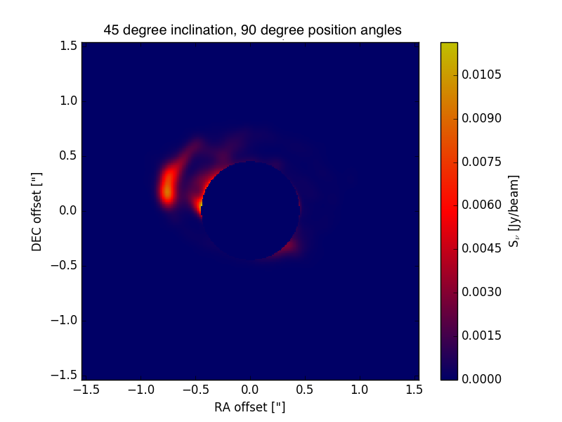
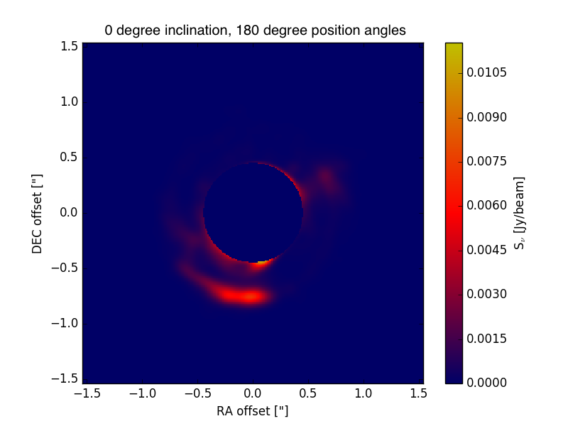
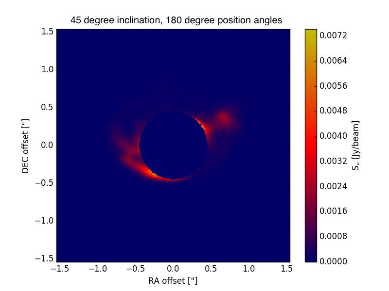
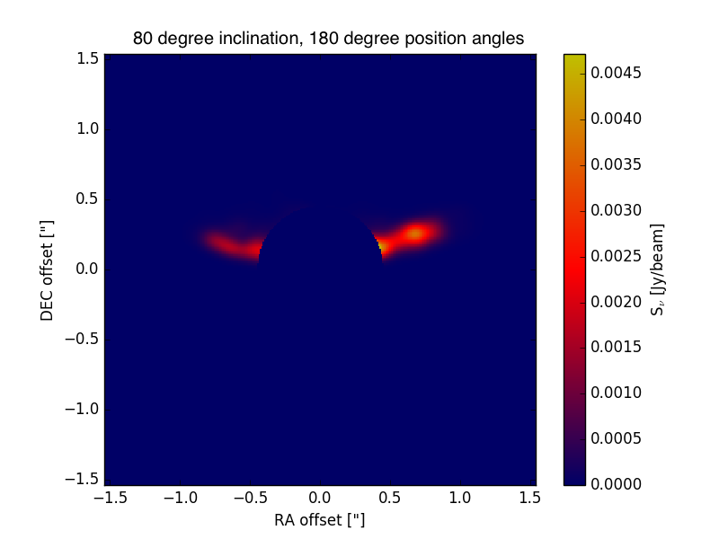
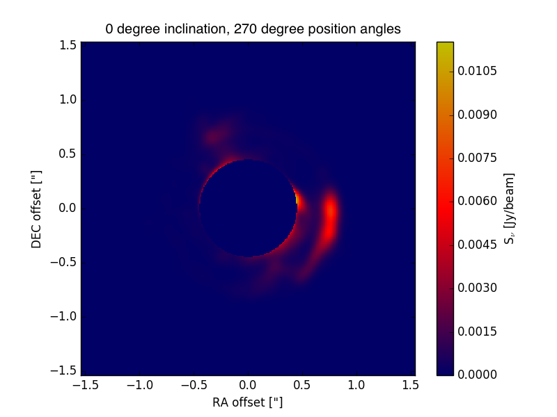
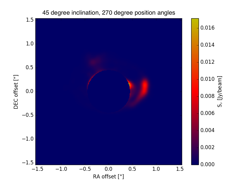
Figure 20.— Array of synthetic images at 10 $\mu$m without scattering included. The original shock heating rate is used. Rows from top to bottom are position angles of 0^∘, 90^∘, 180^∘, and 270^∘. From left to right are inclination angles of 0^∘, 45^∘, and 80^∘.

References

- Baruteau et al. (2014) Baruteau, C. et al. 2014, in Protostars and Planets VI, ed. Henrik Beuther, Ralf S. Klessen, Cornelis P. Dullemond, and Thomas Henning, University of Arizona Press, 667-689
- Bell et al. (1997) Bell, K. R., Cassen, P. M., Klahr, H. H., & Henning, T. 1997, ApJ, 486, 372
- Benisty et al. (2015) Benisty, M. et al. 2015, A&A, 578, L6
- Berriman et al. (1994) Berriman, G. B., Boggess, N. W., Hauser, M. G., Kelsall, T., Lisse, C. M., Moseley, S. H., Reach, W. T., & Silverberg, R. F. 1994, ApJ, 431, L63
- Bjorkman & Wood (2001) Bjorkman, J. E., & Wood, K. 2001, ApJ, 554, 615
- Boley & Durisen (2006) Boley, A. C., & Durisen, R. H. 2006, ApJ, 641, 534
- Brandenburg & Dobler (2002) Brandenburg, A., & Dobler, W. 2002, Computer Physics Communications, 147, 471
- Brandenburg & Dobler (2010) —. 2010, Pencil: Finite-difference Code for Compressible Hydrodynamic Flows, Astrophysics Source Code Library
- Currie et al. (2015) Currie, T., Cloutier, R., Brittain, S., Grady, C., Burrows, A., Muto, T., Kenyon, S. J., & Kuchner, M. J. 2015, ApJ, 814, L27
- Currie et al. (2014) Currie, T. et al. 2014, ApJ, 796, L30
- D’Angelo et al. (2003) D’Angelo, G., Henning, T., & Kley, W. 2003, ApJ, 599, 548
- de Val-Borro et al. (2006) de Val-Borro, M. et al. 2006, MNRAS, 370, 529
- Dong et al. (2016) Dong, R., Fung, J., & Chiang, E. 2016, ApJ, 826, 75
- Dullemond et al. (2012) Dullemond, C. P., Juhasz, A., Pohl, A., Sereshti, F., Shetty, R., Peters, T., Commercon, B., & Flock, M. 2012, RADMC-3D: A multi-purpose radiative transfer tool, Astrophysics Source Code Library
- Fung & Dong (2015) Fung, J., & Dong, R. 2015, ApJ, 815, L21
- Garufi et al. (2013) Garufi, A. et al. 2013, A&A, 560, A105
- Goldreich & Tremaine (1979) Goldreich, P., & Tremaine, S. 1979, ApJ, 233, 857
- Gómez & Cox (2004) Gómez, G. C., & Cox, D. P. 2004, ApJ, 615, 744
- Haugen et al. (2004) Haugen, N. E. L., Brandenburg, A., & Mee, A. J. 2004, MNRAS, 353, 947
- Isella et al. (2010) Isella, A., Natta, A., Wilner, D., Carpenter, J. M., & Testi, L. 2010, ApJ, 725, 1735
- Juhász et al. (2015) Juhász, A., Benisty, M., Pohl, A., Dullemond, C. P., Dominik, C., & Paardekooper, S.-J. 2015, MNRAS, 451, 1147
- Kley (1999) Kley, W. 1999, MNRAS, 303, 696
- Kley & Dirksen (2006) Kley, W., & Dirksen, G. 2006, A&A, 447
- Lee (2016) Lee, W.-K. 2016, ApJ, 832, 166
- Lin & Papaloizou (1979) Lin, D., & Papaloizou, J. 1979, MNRAS, 186, 799
- Lin & Papaloizou (1993) Lin, D. N. C., & Papaloizou, J. C. B. 1993, in Protostars and Planets III, ed. E. H. Levy & J. I. Lunine, 749–835
- Lovelace et al. (1999) Lovelace, R., Li, H., Colgate, S., & Nelson, A. 1999, ApJ, 513, 805
- Lyra et al. (2009) Lyra, W., Johansen, A., Klahr, H., & Piskunov, N. 2009, A&A, 493, 1125
- Lyra & Lin (2013) Lyra, W., & Lin, M.-K. 2013, ApJ, 775, 17
- Lyra et al. (2016) Lyra, W., Richert, A., Boley, A., Turner, N., Mac Low, M.-M., Okuzumi, S., & Flock, M. 2016, ApJ, 817, 102 (Paper II)
- Muto et al. (2012) Muto, T. et al. 2012, ApJ, 748, L22
- Ogilvie & Lubow (2002) Ogilvie, G. I., & Lubow, S. H. 2002, MNRAS, 330, 950
- Papaloizou & Nelson (2005) Papaloizou, J. C. B., & Nelson, R. P. 2005, A&A, 433, 247
- Preibisch et al. (1993) Preibisch, T., Ossenkopf, V., Yorke, H. W., & Henning, T. 1993, A&A, 279, 577
- Rafikov (2002) Rafikov, R. R. 2002, ApJ, 569, 997
- Richert et al. (2015) Richert, A. J. W., Lyra, W., Boley, A., Mac Low, M.-M., & Turner, N. 2015, ApJ, 804, 95 (Paper I)
- van der Marel et al. (2013) van der Marel, N. et al. 2013, Science, 340, 1199
- Zhu et al. (2015) Zhu, Z., Dong, R., Stone, J. M., & Rafikov, R. R. 2015, ApJ, 813, 88,108