Low-temperature anomalies of a vapor deposited glass

Abstract

We investigate the low temperature properties of two-dimensional Lennard-Jones glass films, prepared in silico both by liquid cooling and by physical vapor deposition. We identify deep in the solid phase a crossover temperature $T^{*}$, at which slow dynamics and enhanced heterogeneity emerge. Around $T^{*}$, localized defects become visible, leading to vibrational anomalies as compared to standard solids. We find that on average, $T^{*}$ decreases in samples with lower inherent structure energy, suggesting that such anomalies will be suppressed in ultra-stable glass films, prepared both by very slow liquid cooling and vapor deposition.

Low-temperature crystalline solids are usually described in terms of harmonic vibrations around a perfect periodic lattice (phonons). Within this framework, defects such as vacancies and dislocations can be treated as small perturbations. This description breaks down for amorphous solids such as glasses, foams, emulsions, plastics, colloids, granular materials, bacterial colonies, and tissues Falk and Langer (1998); Schall et al. (2007); Hentschel et al. (2010); Puosi et al. (2016); Keys et al. (2011); Candelier et al. (2010); Cubuk et al. (2015). In these systems, the identification of “defects” becomes challenging because the solid ground state is strongly disordered. As a consequence, amorphous solids display many universal anomalies with respect to crystals. Examples are the so-called Boson Peak, an excess of low-energy vibrational modes Malinovsky and Sokolov (1986); the anomalous scaling of heat capacity and thermal conductivity with temperature Zeller and Pohl (1971); Phillips (1987); the irreversible plastic response to arbitrarily small perturbations Falk and Langer (1998); Malandro and Lacks (1999); Hentschel et al. (2010); Puosi et al. (2016); and highly cooperative relaxation dynamics, contributing to the so-called $\beta$-processes Hachenberg et al. (2008); Goldstein (2010); Capaccioli et al. (2012).

These anomalies have been widely reported in amorphous solids of very different nature. Interestingly, recent experimental work has shown that by preparing glasses through a process of physical vapor deposition, one can produce ultra-stable states that lie deep in the free energy landscape Swallen et al. (2007). Compared to their liquid-cooled counterparts, vapor-deposited glasses show higher density Dalal et al. (2012) and kinetic stability Swallen et al. (2007); Leon-Gutierrez et al. (2010). When these ultra-stable glasses are studied at very low temperatures, it is found that the anomalies characteristic of amorphous solids are strongly supressed Queen et al. (2013); Pérez-Castañeda et al. (2014); Liu et al. (2014); Yu et al. (2015); Tylinski et al. (2016).

Many theoretical approaches to this problem are based on the study of the potential energy landscape of glass-forming particle systems Goldstein (1969); Stillinger and Weber (1983); Sastry et al. (1998); Debenedetti and Stillinger (2001); Heuer (2008); Goldstein (2010); Charbonneau et al. (2014). These studies have suggested that glass anomalies can be interpreted in terms of glass states being not well-defined energy minima, but structured metabasins containing a collection of sub-basins separated by barriers of variable size Reinisch and Heuer (2004); Middleton and Wales (2001), see Fig. 1. In particular, recent work Charbonneau et al. (2015); Berthier et al. (2016); Scalliet et al. (2017) has identified a set of simple observables (the mean square displacement between identical “clones” of the original system) that allows one to detect easily the development of a structure of sub-basins inside a glass metabasin.

In this work, using the methods of Charbonneau et al. (2015); Berthier et al. (2016); Scalliet et al. (2017), we explore in silico the potential energy landscape of binary Lennard-Jones glass films prepared through two experimentally relevant protocols: slow liquid cooling, and physical vapor deposition following Ref. Reid et al. (2016). We study these films due to their experimental relevance and the fact that they have been well characterized by previous work Reid et al. (2016); Helfferich et al. (2016). In contrast to previous studies which prepared bulk equilibrium samples using the swap algorithm Berthier et al. (2016); Scalliet et al. (2017), our film preparation methods –inspired by the vapor-deposition experimental protocol– produce non-equilibrium films that are expected to be higher in the potential energy landscape than experimentally prepared vapor-deposited glasses Ninarello et al. (2017); Berthier et al. (2017). In addition, both our liquid-cooled and vapor-deposited films are prepared in the presence of both a substrate and a free surface, allowing the study of these features’ influence on the low-temperature physics of the samples.

We find that a threshold $T^{*}$ can be detected within the glass phase, below which vibrational dynamics of the solid become orders of magnitude slower and the structure of the glass basin becomes visible. The value of $T^{*}$ depends primarily on film stability, decreasing substantially with the inherent structure energy of the sample - a measure of stability Helfferich et al. (2016) -, while a protocol dependence of $T^{*}$ is not detected. This observation is compatible with the disappearance of anomalies in ultra-stable glasses. Furthermore, we observe significant sample-to-sample variations both in the value of $T^{*}$ and in the aging dynamics below this threshold. All samples display localized defects, however several samples display collective dynamics, which could be related to cooperative displacements enabled by the free surface. It is important to note that the glasses considered here incorporate the non-equilibrium nature of real materials, as well as the presence of a substrate and free boundary, which have an important impact on the physics below $T^{*}$. Note also that the films considered in this study have fixed thickness (the same used in Ref. Reid et al. (2016)), so the dependence of the results on films’ thickness is not addressed here and left for future work.

I Sample preparation protocol

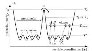
Figure 1: Illustration of the energy landscape. Samples are prepared in a glass basin at temperature $T_{\rm f}$ or $T_{\rm s}$ lower than the glass transition $T_{\rm g}$. They are then brought at lower temperature $T_{\rm clone}$ to ensure that no residual diffusion ($\alpha$-relaxation) is present. There, clones are produced to sample the interior of glass basins. Our main observables are $\Delta(t,t_{\mathrm{w}})$, the mean square displacement of particles in a single clone, and $\Delta_{\rm AB}(t_{\mathrm{w}})$, the displacement between two distinct clones.

Here we provide a brief description of the system and protocols used in this work. See Ref. Reid et al. (2016), the illustration in Fig. 1 and the Appendix for details. We prepare $N_{\rm s}$ glass samples of a binary two-dimensional Lennard-Jones system which shows a glass transition temperature close to $T_{\rm g}\approx 0.21$ for the range of cooling rates used in this study. We study two distinct classes of films: (i) those formed by slow cooling (SC) of liquid films into the glass phase at a final temperature $T_{\rm f}$ with two distinct cooling rates $\delta_{\mathrm{SC}}$, and (ii) those formed by a procedure mimicking physical vapor deposition (VD). In VD, we use four different deposition rates $\delta_{\mathrm{VD}}$ with substrates held at temperature $T_{\rm s}$. In both protocols, $T_{\rm f}<T_{\rm g}$ or $T_{\rm s}<T_{\rm g}$, so the samples we produce are in the glass phase.

To study the vibrational anomalies of a glass basin, each sample is brought to a lower temperature $T_{\rm clone}$ (lower than either $T_{\rm f}$ or $T_{\rm s}$). The same $T_{\rm clone}$ is employed in all cases, i.e. for all samples and all protocols. At this temperature the system is sufficiently close to its inherent structure. In fact, as shown in Fig. 2a, the inherent structure energy (as computed by energy minimization configurations at different temperatures) remains constant below this temperature for all the glasses considered. From this, we suggest that no diffusion occurs over this period. We verify that the system behaves as a normal solid at $T_{\rm clone}$, meaning that the state is ergodic and the vibrations of the particles are weakly correlated. Once cooled, we prepare $N_{\rm c}$ clones, or independent configurations distributed within the basin of each glass sample. In practice, each clone is obtained as the result of an independent simulation of length $t_{\mathrm{clones}}$, the dotted line in Fig. 2.

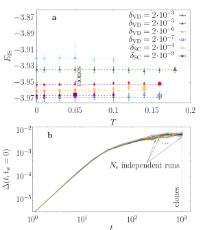
Figure 2: Preparation of glass samples and clones. (a) Inherent structure energy $E_{\mathrm{IS}}$ measured at $T_{\rm f}$ or $T_{\rm s}$ (larger symbol), and upon cooling or heating the samples at different $T$. Dashed lines are constant fits to the data for $T\leq T_{\rm clone}=0.05$, that demonstrate that the system is not leaving its metabasin. (b) $\Delta(t,t_{\mathrm{w}}=0)$ at temperature $T=T_{\rm clone}$ for one of the VD samples prepared with $\delta_{\mathrm{VD}}=2\cdot 10^{-6}$. The length of the clone preparation simulations is indicated by the dotted line, whose length is the size of the cage (i.e. the height of the plateau).

The clones are then instantaneously quenched to a final temperature $T<T_{\rm clone}$ and their dynamics are examined at constant $T$, with $t_{\mathrm{w}}$ being the time elapsed since the quench. Note that when samples are studied at $T=T_{\rm clone}$, the dynamics are stationary, and for this reason the origin of time can be chosen arbitrarily.

Following previous work Charbonneau et al. (2015); Berthier et al. (2016); Scalliet et al. (2017), we focus our attention on two observables:

$$\Delta(t+t_{\mathrm{w}},t_{\mathrm{w}})=\frac{1}{N}\sum_{i=1}^{N}\overline{{\left\langle{|\bm{r}_{i}(t+t_{\mathrm{w}})-\bm{r}_{i}(t_{\mathrm{w}})|^{2}}\right\rangle}}\ ,$$ (1)

which is the mean square displacement of particles in each clone between time $t_{\mathrm{w}}$ and $t+t_{\mathrm{w}}$, and

$$\Delta_{\rm AB}(t_{\mathrm{w}})=\frac{1}{N}\sum_{i=1}^{N}\overline{{\left\langle{|\bm{r}_{i}^{A}(t_{\mathrm{w}})-\bm{r}_{i}^{B}(t_{\mathrm{w}})|^{2}}\right\rangle}}\ .$$ (2)

which is the mean square displacement between particles in two distinct clones (denoted A and B) of the same sample at the same time $t_{\mathrm{w}}$, $\{\bm{r}_{i}^{A}(t_{\mathrm{w}})\}$ and $\{\bm{r}_{i}^{B}(t_{\mathrm{w}})\}$. Here, ${\left\langle{\ \bullet\ }\right\rangle}$ refers to the thermal average, computed as the average over all the clones of the same sample, while $\overline{\ \bullet\ }$ refers to the average over all the samples with the same preparation procedure. To increase the statistics, the thermal average of $\Delta_{\rm AB}$ is computed using all the $N_{\mathrm{c}}(N_{\mathrm{c}}-1)/2$ possible couples of A and B clones, but the error bars are computed by taking into account the correlations between pairs using the jack-knife method Amit and Martin-Mayor (2005).

Both quantities are computed for particles in the middle region of the sample (the region in between the two horizontal lines in Fig. 8). In this region the density and relative concentration of the two particle types are both constant Reid et al. (2016), allowing boundary effects to be avoided. The displacement of the center of mass of the whole sample is removed. Both observables are averaged over clones and, unless otherwise specified, over multiple samples prepared with the same protocol.

II Results

II.1 Clones are prepared in an ergodic state

We begin by discussing the behavior of $\Delta(t+t_{\mathrm{w}},t_{\mathrm{w}})$ and $\Delta_{\rm AB}(t_{\mathrm{w}})$ for samples at the clone preparation temperature $T_{\rm clone}$ (see purple squares in Fig. 3). Because clones have been prepared well below $T_{g}$, no diffusion is observed in our simulation time windows, meaning that the averaged cage size $\Delta^{\infty}$ of the material at each temperature can be extracted from the plateau value of $\Delta(t+t_{\mathrm{w}},t_{\mathrm{w}})$ at long $t_{\mathrm{w}}$, as shown in Fig. 3a. On the other hand, $\Delta_{\rm AB}(t_{\mathrm{w}})$ reach a constant value at long times, see Fig. 3b, that precisely coincides with $\Delta^{\infty}$ (it can be better appreciated in Fig. 4b where both observables are plotted superimposed). The convergence of these two quantities in the long time limit means that a single trajectory of the system samples, at long times, the same states that are sampled by two independently prepared clones. This indicates that the glass basin is comprised of well-defined internal cages which are ergodically sampled, and that vibrations of particles remain weaky correlated Berthier et al. (2016); Seguin and Dauchot (2016); Scalliet et al. (2017).

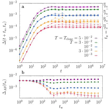
Figure 3: Emergence of slow vibration dynamics. (a) Aging effects in ${\Delta(t+t_{\mathrm{w}},t_{\mathrm{w}})}$ for VD glasses obtained with $\delta_{\mathrm{VD}}=2\cdot 10^{-6}$. For each temperature we plot four values of $t_{\mathrm{w}}$ ($2^{16},2^{18},2^{20},2^{22}$), all of them corresponding to the regime where the ballistic part has converged to the same curve. (b) Aging effects in $\Delta_{\mathrm{AB}}(t_{\mathrm{w}})$.

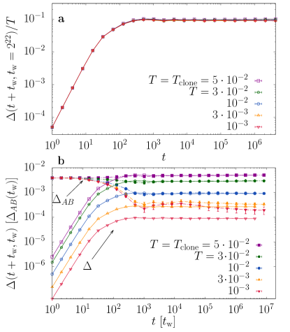
Figure 4: Breakdown of the ergodicity. (a) The scaled $\Delta(t+t_{\mathrm{w}},t_{\mathrm{w}})/T$ for the largest $t_{\mathrm{w}}=2^{22}$, at different temperatures. There is an excellent collapse indicating that for large $t_{\mathrm{w}}$ the MSD is proportional to temperature. (b) We compare $\Delta(t+t_{\mathrm{w}},t_{\mathrm{w}})$ for $t_{\mathrm{w}}=2^{22}$ vs. $t$ with $\Delta_{\mathrm{AB}}(t_{\mathrm{w}})$ vs. $t_{\mathrm{w}}$ of Fig. 3. The onset where $\Delta_{\rm AB}^{\infty}=\Delta_{\rm AB}(t_{\mathrm{w}}\to\infty)\neq\Delta(t\to\infty,t_{\mathrm{w}}\to\infty)=\Delta^{\infty}$ corresponds to the emergence of aging of Fig. 3a.

II.2 Growing timescales upon cooling

Next, we study the behavior of $\Delta(t+t_{\mathrm{w}},t_{\mathrm{w}})$ and $\Delta_{\rm AB}(t_{\mathrm{w}})$ as a function of $t$, using different reference times $t_{\mathrm{w}}$ elapsed after a sudden drop in temperature from $T_{\rm clone}$ to $T<T_{\rm clone}$ (Fig. 3). At small values of $t_{\mathrm{w}}$, one expects a sharp nonequilibrium response of $\Delta(t+t_{\mathrm{w}},t_{\mathrm{w}})$ and $\Delta_{\rm AB}(t_{\mathrm{w}})$ to the change of temperature: this is manifested both at small $t$, during the ballistic exploration of the cages, and at long $t$ in the plateau region. The value of the plateau evolves from the typical cage size at the preparation temperature (at very small $t_{\mathrm{w}}$), to the new temperature one (longest $t_{\mathrm{w}}$), see Fig. 3. In addition, as we show in Fig. 4a, the limiting long-$t_{\mathrm{w}}$ curves at different temperatures can be roughly collapsed in a single curve by dividing them by the temperature, which suggests that the size of the cages increases linearly with temperature. However, the typical time it takes to the system to converge to this long-$t_{\mathrm{w}}$ plateau, depends drastically on the final temperature. This is more clearly seen by plotting $\Delta(t+t_{\mathrm{w}},t_{\mathrm{w}})/T$ for $t=2^{22}$ [i.e. the long $t$ limit of the mean-squared displacement (MSD)] as function of $t_{\mathrm{w}}$, see Fig. 5a. While at high temperatures the plateau converges rapidly to its final value, this convergence slows significantly as the temperature is decreased. In order to quantify this effect, we extract the time $\tau$ such that for $t_{\mathrm{w}}>\tau$, the value of $\Delta(2^{22}+t_{\mathrm{w}},t_{\mathrm{w}})/T$ is consistently below a threshold (dashed line in Fig. 5a). We fixed the threshold to 0.2 for all the samples. The errors are obtained using the jack-knife method Amit and Martin-Mayor (2005). We show $\tau$ as a function of $T$, for glasses prepared by different protocols in Fig. 5b, finding that these characteristic times grow very quickly in the vicinity of well defined temperatures that depend on how the material was prepared. Of course, within this approach, the values of $\tau$ depend of the threshold chosen, and we observed that the temperatures at which the sharp growth occurs also shift mildly (effect included in the error bars). Nevertheless, the overall picture remains the same.

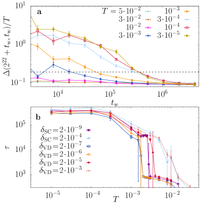
Figure 5: Convergence to the plateau. (a) The plateau height (long $t$ limit of $\Delta(t+t_{\mathrm{w}},t_{\mathrm{w}})/T$, estimated by the largest available $t$) as function of $t_{\mathrm{w}}$ for different temperatures, extracted from the data of Fig. 4a. (b) The time $\tau$ needed to fall below the dashed line in (a), as a function of $T$ for differently prepared glasses.

Furthermore, the convergence to the final cage sizes (Fig. 3a) slows at roughly the same temperatures at which $\Delta(t+t_{\mathrm{w}},t_{\mathrm{w}})$ and $\Delta_{\rm AB}(t_{\mathrm{w}})$ no longer converge to the same plateau value at long times, as shown in Fig. 4b. The large time limit of both quantities, which we call $\Delta^{\infty}$ and $\Delta_{\rm AB}^{\infty}$, plotted as a function of $T$ (Fig. 6b), converge to the same values at high temperatures ($T\gtrsim 10^{-2}$), while they clearly separate at low temperatures. It is however important to note that the relaxation time $\tau$ (Fig. 5b) does not seem to diverge at any finite temperature: instead, it saturates. One may wonder whether this saturation is simply due to the finite size of the system, in which case the value of $\tau$ at low temperature would increase with system size. Ruling out this possibility would require a careful finite size study, that we leave for future work.

II.3 Temperature threshold and inherent structure energy

We have seen that the long time limits $\Delta^{\infty}$ and $\Delta_{\rm AB}^{\infty}$ separate near a threshold $T^{*}$, indicating a loss of ergodicity within the glass basin below this temperature, which is also associated with the emergence of much slower aging dynamics. If we examine each sample individually, we find that the value of $T^{*}$ fluctuates strongly from sample to sample (Fig. 6a), and it depends strongly on how the sample was prepared, as we show in Fig. 6b by taking the sample averages.

To study systematically the dependence of $T^{*}$ on sample preparation method and rate, we define it more precisely as follows. We compute the temperature below which $\Delta^{\infty}$ and $\Delta_{\mathrm{AB}}^{\infty}$ become distinct in each sample, and the temperature for which $\Delta^{\infty}(T)=\Delta^{\infty}_{\mathrm{AB}}(T=10^{-5})$, i.e. the point at which a horizontal line equal to the zero-temperature value of $\Delta_{\rm AB}^{\infty}$ intersects $\Delta^{\infty}(T)$. We define $T^{*}$ as the average of these two estimations (indicated by the arrows in Fig. 6a), and we associate to it an error given by half the difference of these two estimations. The reason for this is that $T^{*}$ does not correspond to a sharp phase transition but rather to a crossover, therefore one cannot define $T^{*}$ unambiguously. We show the results for the $T^{*}$ of each sample in Fig. 6c as function of their inherent structure energy, which is correlated with the cooling or deposition rate and is a proxy for glass stability Reid et al. (2016); Helfferich et al. (2016). In spite of the large spread of the data points, we find that the values of $T^{*}$ are correlated (the linear correlation coefficient is 0.67) with the logarithm of the inherent structure energies of the samples, suggesting that the threshold temperature $T^{*}$ decreases with the inherent structure energy (roughly exponentially). Based on this finding, we suggest that experimental ultrastable glasses, that typically lie in energy minima below the ones accessible in our numerical simulations, would see the anomalies discussed in this work strongly suppressed, as in that case $T^{*}$ would be extremely low or even absent.

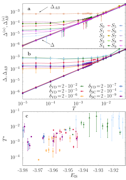
Figure 6: Exponential decay of $T^{*}$ with the inherent structure energy of the samples. (a) Individual long time values of $\Delta^{\infty}$ and $\Delta^{\infty}_{\rm AB}$, plotted versus $T$, for the 10 VD glass samples obtained with $\delta_{\mathrm{VD}}=2\cdot 10^{-6}$. The separation of $\Delta^{\infty}$ and $\Delta^{\infty}_{\rm AB}$ happens at a strongly sample-dependent temperature. (b) Averages of $\Delta^{\infty}$ and $\Delta^{\infty}_{\rm AB}$ over samples, plotted versus $T$, for different sample preparation protocols, showing that the average separation temperature depends on the preparation protocol and decreases for slower protocols. (c) Values of $T^{*}$ as function of the inherent structure energy, as extracted sample by sample for the different preparation protocols (different colors with the same color code as in panel b), showing a high correlation between $E_{\mathrm{IS}}$ and $T^{*}$.

II.4 Aging and heterogeneity of individual samples

We now investigate in greater detail the behavior of individual samples in the regime of times and temperatures where aging dynamics are slow. To this end, in addition to the mean square displacements defined above, we introduce the displacement of individual particles in two clones, $u_{i}(t_{\mathrm{w}})\propto|\bm{r}_{i}^{A}(t_{\mathrm{w}})-\bm{r}_{i}^{B}(t_{\mathrm{w}})|^{2}$, normalized in such a way that $(1/N)\sum_{i}{\left\langle{u_{i}(t_{\mathrm{w}})}\right\rangle}=1$, and following Ref. Scalliet et al. (2017) we introduce a susceptibility

$$\chi_{\rm AB}(t_{\mathrm{w}})=\frac{\sum_{ij}[{\left\langle{u_{i}(t_{\mathrm{w}})u_{j}(t_{\mathrm{w}})}\right\rangle}-{\left\langle{u_{i}(t_{\mathrm{w}})}\right\rangle}{\left\langle{u_{j}(t_{\mathrm{w}})}\right\rangle}]}{\sum_{i}[{\left\langle{u_{i}(t_{\mathrm{w}})^{2}}\right\rangle}-{\left\langle{u_{i}(t_{\mathrm{w}})}\right\rangle}^{2}]}\ ,$$ (3)

that is equal to 1 if $u_{i}(t_{\mathrm{w}})$ and $u_{j}(t_{\mathrm{w}})$ are uncorrelated for all $i\neq j$, while otherwise it gives an estimate of the correlation length of particle displacements (raised to an unknown power). It has been suggested by previous work Charbonneau et al. (2014, 2015); Berthier et al. (2016) that, below the threshold $T^{*}$, the system might be “marginally stable”, i.e. characterized by a diverging correlation length of particle displacements, and a diverging $\chi_{\rm AB}$, also associated to delocalized soft vibrational modes Liu et al. (2011); Müller and Wyart (2015). However, Ref. Scalliet et al. (2017) found, in a system similar to ours, that $\chi_{\rm AB}$ always remains small, suggesting that the low temperature phase is not marginally stable.

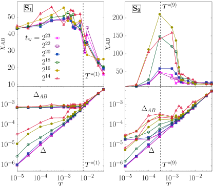
Figure 7: Aging behavior of two representative samples. Values of $\chi_{\rm AB}(t_{\mathrm{w}})$ (top), and of $\Delta_{\rm AB}(t_{\mathrm{w}})$, $\Delta(2^{22}+t_{\mathrm{w}},t_{\mathrm{w}})$ (bottom) for two representative VD samples obtained with $\delta_{\mathrm{VD}}=2\cdot 10^{-6}$, plotted as a function of temperature $T$ for several values of $t_{\mathrm{w}}$. The two samples (labeled 1 and 9) have $e_{IS}^{(1)}=-3.9522$ and $e_{IS}^{(9)}=-3.9628$. Sample 1 displays no aging besides the one related to the convergence of $\Delta(2^{22}+t_{\mathrm{w}},t_{\mathrm{w}})$ to its long time limit at low $T$ and only a moderate increase of $\chi_{\rm AB}$ upon lowering temperature. Sample 9 displays strong aging around its $T^{*(9)}$, accompanied by a large growth of $\chi_{\rm AB}$.

In Fig. 7 we report the aging behavior of $\Delta_{\rm AB}(t_{\mathrm{w}})$ and $\chi_{\rm AB}(t_{\mathrm{w}})$ for two individual representative samples, labeled as sample 1 and sample 9. In sample 1, we do not observe aging in either $\Delta_{\rm AB}(t_{\mathrm{w}})$ or $\chi_{\rm AB}(t_{\mathrm{w}})$, which are independent of $t_{\mathrm{w}}$. The susceptibility displays only a moderate increase upon decreasing temperature below $T^{*(1)}$, which is consistent with the results of Ref. Scalliet et al. (2017). In sample 9, instead, we observe strong aging in $\Delta_{\rm AB}(t_{\mathrm{w}})$ around $T^{*(9)}$, and correspondingly the susceptibility increases by a factor of about 20 at intermediate times and $T\sim T^{*(9)}$, before relaxing to smaller values at longer times.

To provide a real space interpretation of these findings, in Fig. 8 we display snapshots of the displacement field ${\left\langle{u_{i}(t_{\mathrm{w}})}\right\rangle}$, averaged over clones, for the same two representative samples, at several values of $T$ and $t_{\mathrm{w}}$. Both samples display, during the aging, a collective displacement of the upper part of the sample, corresponding to a global increase of density upon cooling –an effect related to the existence of a free surface–, as well as clearly visible localized defects. The main difference between the two samples is that in sample 9 the surface process leads to greater displacement between clones, indicating that this process happens in a more heterogeneous way from clone to clone, leading to the stronger aging visible in both $\Delta_{\rm AB}$ and $\chi_{\rm AB}$. The localized defects are compatible with those observed in Ref. Scalliet et al. (2017) and lead to a separation of $\Delta^{\infty}$ and $\Delta^{\infty}_{\rm AB}$ at low temperatures that is not accompanied by aging nor by a large $\chi_{\rm AB}$. We thus conclude that the system is not marginally stable below $T^{*}$.

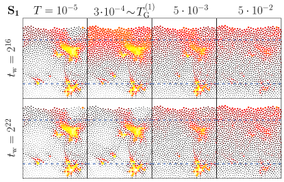
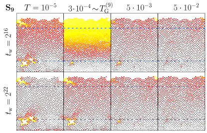
Figure 8: Snapshots of the displacement field. The displacement field ${\left\langle{u_{i}(t_{\mathrm{w}})}\right\rangle}$, averaged over clones, is shown for the same two representative samples as in Fig. 7. For each particle $i$, the corresponding displacement is shown as a circle centered in the particle position, whose area is proportional to ${\left\langle{u_{i}(t_{\mathrm{w}})}\right\rangle}$. The colors help visualising the largest displacements. Sample 1 displays only localized defects, while sample 9 displays, at intermediate times and $T\sim T^{*(9)}$, a collective displacement of the upper part of the sample.

III Discussion

We have identified, independently for each sample (or glass basin), a threshold temperature $T^{*}$, located deep in the glass phase. Around this temperature, the aging dynamics after a quench becomes slow, and vibrational heterogeneity is enhanced. Below $T^{*}$, aging dynamics remains slow, and localized defects appear, similar to the ones reported in Refs. Scalliet et al. (2017); Hicks et al. (2017). The threshold, however, does not correspond to a sharp phase transition and excitations are localized below $T^{*}$.

Our main result is that $T^{*}$ markedly decreases with decreasing $E_{\rm IS}$ and thus increasing film stability Reid et al. (2016); Helfferich et al. (2016). Hence, ultra-stable glasses with low $E_{\rm IS}$ are also predicted to display a very low $T^{*}$ and thus remain normal solids down to extremely low temperatures. Our results qualitatively agree with previous studies Berthier et al. (2016); Scalliet et al. (2017), but they are obtained for non-equilibrium films, formed through realistically simulated liquid cooling and physical vapor deposition processes, that sit higher in the energy landscape Berthier et al. (2017).

The theoretical interpretation of our findings is challenging. Localized defects of different nature have been discussed in the context of glasses, see e.g. Lerner et al. (2016); Mizuno et al. (2017); Keys et al. (2011); Candelier et al. (2010); Cubuk et al. (2015); Jack and Garrahan (2016); Falk and Langer (1998); Schall et al. (2007); Lubchenko and Wolynes (2003); Hentschel et al. (2010); Puosi et al. (2016), and our findings could be related to at least some of those theoretical proposals. Future work should clarify these connections, both by additional numerical simulations and analytical calculations. The emergence of slow dynamics at low temperature, accompanied by the non-trivial change in the vibrations of the particles, is reminiscent of the mean field scenario where these features are consequences of an underlying phase transition, called the Gardner transition Gardner (1985); Charbonneau et al. (2017), which separates a high-temperature normal solid and a low-temperature marginally stable solid. While our results, similarly to the ones of Ref. Scalliet et al. (2017); Hicks et al. (2017) suggest that no sharp phase transition takes place in our samples, one could speculate that the localized excitations we identified are some kind of “vestige” of an avoided Gardner-like transition. Because numerical simulations of hard sphere (colloidal) glasses are instead consistent with the existence of a transition Berthier et al. (2016), it becomes very important to understand which systems display such a transition and which do not, and why. This is a very important direction for future work, both analytical Urbani and Biroli (2015); Larson et al. (2013); Angelini and Biroli (2015); Aspelmeier et al. (2016); Charbonneau and Yaida (2017), numerical Baity-Jesi et al. (2014); Charbonneau et al. (2015); Berthier et al. (2016); Scalliet et al. (2017); Hicks et al. (2017) and experimental Seguin and Dauchot (2016); Geirhos et al. (2017).

In conclusion, our observations may explain why some anomalies characteristic of amorphous solids are suppressed in ultra-stable glasses, but more work is needed to relate precisely the anomalies observed in our numerically simulated samples to the ones observed in experiments Queen et al. (2013); Pérez-Castañeda et al. (2014); Liu et al. (2014); Yu et al. (2015); Tylinski et al. (2016). Moreover, finite size effects, and in particular the dependence of our results on films’ thickness, remain to be investigated.

Appendix A Details of the system

We work with films of a binary mixture of $N=1200$, two-dimensional Lennard-Jones particles of type 1 and 2 (where 1 is more common with concentration $\chi_{1}\equiv N_{1}/N\sim 65\%$) that interact with a third type of particles 3 that act as a fixed substrate at the bottom of the simulation box. The upper boundary in the vertical axis remains open and we consider periodic boundary conditions in the direction parallel to the substrate. The interaction potential between particles of two species $\alpha,\beta$ separated by a distance $r$ is

$$u_{\alpha,\beta}(r)=4\epsilon_{\alpha,\beta}\left[{\left({\frac{\sigma_{\alpha,\beta}}{r}}\right)^{12}-\left({\frac{\sigma_{\alpha,\beta}}{r}}\right)^{6}}\right]\ ,$$ (4)

for $r<r_{\mathrm{cutoff}}^{\alpha,\beta}$, and zero otherwise. The cutoff distances are $r_{\mathrm{cutoff}}^{\alpha,\beta}=2.5\sigma_{\alpha,\beta}$, being the particle diameters, $\sigma_{11}=1.0\sigma$, $\sigma_{22}=0.88\sigma$, $\sigma_{33}=0.6\sigma$, $\sigma_{12}=0.8\sigma$, $\sigma_{13}=0.75\sigma$, $\sigma_{23}=0.75\sigma$. For the potential we use the values $\epsilon_{11}=1.0\epsilon$, $\epsilon_{22}=0.5\epsilon$, $\epsilon_{33}=0.1\epsilon$, $\epsilon_{12}=1.5\epsilon$, $\epsilon_{13}=1.0\epsilon$, $\epsilon_{23}=1.0\epsilon$. All quantities in the paper are shown in Lennard-Jones units, that is: $\sigma$, $\epsilon$ and mass $m$ are equal to 1, and time is thus in units of $\sigma\sqrt{m/\epsilon}$. Energies in the paper were measured without shifting the potential to zero at the cutoff distance, a choice that has no impact during the simulation considering that updates in the molecular dynamics algorithm only depend on the derivatives of the interaction potential $u_{\alpha,\beta}(r)$. The discrepancies between the inherent structure energies of this work and the ones shown in Ref. Reid et al. (2016) come from the fact that in the previous work energies were rescaled to compare configurations with exactly the same portion of type-1 particles in the bulk. The temperature is fixed using a Nosé-Hoover thermostat Martyna et al. (1992) with a temperature damping parameter $100\Delta t$, where the time step is here $\Delta t=0.005$. Inherent structural energies were calculated by minimizing configurations using the FIRE algorithm with energy and force tolerances of $10^{-10}$ Bitzek et al. (2006). All simulations were performed using LAMMPS Plimpton (1995).

Because $\epsilon_{12}$ is higher than $\epsilon_{11}$ and $\epsilon_{22}$, the most stable configurations tend to maximize the $1-2$ interactions, which, considering that $1$ particles are more abundant, tends to displace the particles of type $1$ towards the surface, creating a clear non-homogeneity along the axis perpendicular to the substrate. In order to avoid the effect of these two boundaries, all the quantities computed in this paper were measured using only the particles in bulk, which corresponds to the central 60% region (see for example the region in between the two horizontal lines in Fig. 8 of the main text). The number of particles in the bulk varies from sample to sample, but it remains equal to $N_{\mathrm{bulk}}\sim 660-670$.

Appendix B Preparation of glass samples

We prepare glass configurations following two distinct protocols: slow cooling from the liquid phase (SC) with two distinct cooling rates $\delta_{\mathrm{SC}}=2\cdot 10^{-4}$ and $\delta_{\mathrm{SC}}=2\cdot 10^{-9}$ down to $T_{\rm f}=0.05$, and a protocol mimicking the vapor deposition (VD) procedure using four different particle-deposition rates $\delta_{\mathrm{VD}}$ with substrates at different temperatures $T_{\rm s}$. The details concerning this protocol can be found in Ref. Reid et al. (2016); we selected for each deposition rate $\delta_{\mathrm{VD}}$ the value of $T_{\rm s}$ that corresponds to the lowest inherent structure energy of the resulting glass, which gives $T_{\rm s}=0.18$ at $\delta_{\mathrm{VD}}=2\cdot 10^{-3}$, $T_{\rm s}=0.16$ at $\delta_{\mathrm{VD}}=2\cdot 10^{-5}$, $T_{\rm s}=0.14$ at $\delta_{\mathrm{VD}}=2\cdot 10^{-6}$, and $T_{\rm s}=0.16$ at $\delta_{\mathrm{VD}}=2\cdot 10^{-7}$.

Following each protocol, we prepare $N_{\mathrm{s}}$ independent glasses (to which we will refer here as samples), each corresponding to a distinct glass basin in the energy landscape. We have considered $N_{\mathrm{s}}=10$ for all the cases with the exception of the VD glasses obtained with the slowest particle deposition rate, where only $5$ samples were considered. We define the inherent structure (IS) of a configuration as the energy minimum that is reached by minimizing the energy starting from that configuration Stillinger and Weber (1982). The different protocols allow us to produce glasses with a wide range of inherent structure energies $E_{\mathrm{IS}}$ (Fig. 1b in the main text).

Appendix C Cloning procedure

To study the vibrational anomalies of a glass basin, for each of these samples, we create $N_{\mathrm{c}}$ clones, which correspond to different configurations of the same glass state, using the following procedure:

• We first cool the initial configuration instantaneously to $T=T_{\rm clone}=0.05$, and let it relax until we observe no more aging in the height of the plateau (during $2^{14}$ time steps). This temperature is chosen because for $T<T_{\rm clone}$, $E_{\mathrm{IS}}$ becomes independent of temperature for all the samples, and furthermore no diffusion is observed at $T_{\rm clone}$ (with the exception of the samples prepared by the fastest cooling and deposition rates, i.e. $\delta_{\mathrm{SC}}=2\cdot 10^{-4}$ and $\delta_{\mathrm{VD}}=2\cdot 10^{-3}$ respectively, where some diffusion is still observed at this temperature at long times). These two observations imply that at $T_{\rm clone}$ the configurations are trapped into well-defined glass basins, which is not always the case at the preparation temperature ($T_{\rm f}$ or $T_{\rm s}$ depending on the protocol), where residual diffusion and inherent structure energy variations are observed in some samples.

• Stable glass configurations obtained at $T_{\rm clone}$ are then cloned by performing $N_{\mathrm{c}}=200$ short independent simulations assigning to each configuration a set of independent random velocities drawn from the Maxwell distribution at $T_{\rm clone}$, as shown in the inset of Fig. 1 in the main text. The length of these simulations is chosen to be longer than the ballistic regime, to let the particles explore their inner cages (of average sizes $\Delta^{\infty}$). In our case, $2^{10}$ (the vertical dotted line in Fig. 2a in the main text) satisfied these requirements for all our samples.

The clones thus represent independent configurations of a same sample at the cloning temperature $T_{\rm clone}$.

Appendix D Instantaneous quenches in temperature

Now starting from each of these clones, we perform instantaneous quenches to lower temperatures. That is, we rescale the velocities of the particles in such a way that the kinetic energy corresponds to a temperature $T<T_{\rm clone}$, and then we use standard molecular dynamics to follow the evolution of the system, keeping the temperature fixed by a Nosé-Hoover thermostat Martyna et al. (1992). The initial time corresponds to the time of the quench, and we call $t_{\mathrm{w}}$ the time elapsed since the quench.

References

- Falk and Langer (1998) M. L. Falk and J. S. Langer, Phys. Rev. E 57, 7192 (1998).
- Schall et al. (2007) P. Schall, D. A. Weitz, and F. Spaepen, Science 318, 1895 (2007).
- Hentschel et al. (2010) H. G. E. Hentschel, S. Karmakar, E. Lerner, and I. Procaccia, Phys. Rev. Lett. 104, 025501 (2010).
- Puosi et al. (2016) F. Puosi, J. Rottler, and J.-L. Barrat, Phys. Rev. E 94, 032604 (2016).
- Keys et al. (2011) A. S. Keys, L. O. Hedges, J. P. Garrahan, S. C. Glotzer, and D. Chandler, Phys. Rev. X 1, 021013 (2011).
- Candelier et al. (2010) R. Candelier, A. Widmer-Cooper, J. K. Kummerfeld, O. Dauchot, G. Biroli, P. Harrowell, and D. R. Reichman, Phys. Rev. Lett. 105, 135702 (2010).
- Cubuk et al. (2015) E. D. Cubuk, S. S. Schoenholz, J. M. Rieser, B. D. Malone, J. Rottler, D. J. Durian, E. Kaxiras, and A. J. Liu, Phys. Rev. Lett. 114, 108001 (2015).
- Malinovsky and Sokolov (1986) V. K. Malinovsky and A. P. Sokolov, Solid State Commun. 57, 757 (1986).
- Zeller and Pohl (1971) R. Zeller and R. Pohl, Phys. Rev. B 4, 2029 (1971).
- Phillips (1987) W. A. Phillips, Rep. Prog. Phys. 50, 1657 (1987).
- Malandro and Lacks (1999) D. L. Malandro and D. J. Lacks, J. Chem. Phys. 110, 4593 (1999).
- Hachenberg et al. (2008) J. Hachenberg, D. Bedorf, K. Samwer, R. Richert, A. Kahl, M. D. Demetriou, and W. L. Johnson, Applied Physics Letters 92, 131911 (2008).
- Goldstein (2010) M. Goldstein, The Journal of Chemical Physics 132, 041104 (2010).
- Capaccioli et al. (2012) S. Capaccioli, M. Paluch, D. Prevosto, L.-M. Wang, and K. Ngai, The Journal of Physical Chemistry Letters 3, 735 (2012).
- Swallen et al. (2007) S. F. Swallen, K. L. Kearns, M. K. Mapes, Y. S. Kim, R. J. McMahon, M. D. Ediger, T. Wu, L. Yu, and S. Satija, Science 315, 353 (2007).
- Dalal et al. (2012) S. S. Dalal, A. Sepúlveda, G. K. Pribil, Z. Fakhraai, and M. Ediger, The Journal of chemical physics 136, 204501 (2012).
- Leon-Gutierrez et al. (2010) E. Leon-Gutierrez, A. Sepúlveda, G. Garcia, M. T. Clavaguera-Mora, and J. Rodríguez-Viejo, Physical chemistry chemical physics 12, 14693 (2010).
- Queen et al. (2013) D. R. Queen, X. Liu, J. Karel, T. H. Metcalf, and F. Hellman, Phys. Rev. Lett. 110, 135901 (2013).
- Pérez-Castañeda et al. (2014) T. Pérez-Castañeda, C. Rodríguez-Tinoco, J. Rodríguez-Viejo, and M. A. Ramos, Proceedings of the National Academy of Sciences 111, 11275 (2014).
- Liu et al. (2014) X. Liu, D. R. Queen, T. H. Metcalf, J. E. Karel, and F. Hellman, Physical review letters 113, 025503 (2014).
- Yu et al. (2015) H. B. Yu, M. Tylinski, A. Guiseppi-Elie, M. D. Ediger, and R. Richert, Physical review letters 115, 185501 (2015).
- Tylinski et al. (2016) M. Tylinski, Y. Chua, M. Beasley, C. Schick, and M. Ediger, The Journal of chemical physics 145, 174506 (2016).
- Goldstein (1969) M. Goldstein, J. Chem. Phys. 51, 3728 (1969).
- Stillinger and Weber (1983) F. H. Stillinger and T. A. Weber, Phys. Rev. A 28, 2408 (1983).
- Sastry et al. (1998) S. Sastry, P. G. Debenedetti, and F. H. Stillinger, Nature 393, 554 (1998).
- Debenedetti and Stillinger (2001) P. G. Debenedetti and F. H. Stillinger, Nature 410, 259 (2001).
- Heuer (2008) A. Heuer, Journal of Physics: Condensed Matter 20, 373101 (2008).
- Charbonneau et al. (2014) P. Charbonneau, J. Kurchan, G. Parisi, P. Urbani, and F. Zamponi, Nature Communications 5, 3725 (2014).
- Reinisch and Heuer (2004) J. Reinisch and A. Heuer, Physical Review B 70, 064201 (2004).
- Middleton and Wales (2001) T. F. Middleton and D. J. Wales, Physical Review B 64, 024205 (2001).
- Charbonneau et al. (2015) P. Charbonneau, Y. Jin, G. Parisi, C. Rainone, B. Seoane, and F. Zamponi, Phys. Rev. E 92, 012316 (2015).
- Berthier et al. (2016) L. Berthier, P. Charbonneau, Y. Jin, G. Parisi, B. Seoane, and F. Zamponi, Proceedings of the National Academy of Sciences 113, 8397 (2016).
- Scalliet et al. (2017) C. Scalliet, L. Berthier, and F. Zamponi, Phys.Rev.Lett. 119, 205501 (2017).
- Reid et al. (2016) D. R. Reid, I. Lyubimov, M. Ediger, and J. J. De Pablo, Nature Communications 7 (2016).
- Helfferich et al. (2016) J. Helfferich, I. Lyubimov, D. Reid, and J. J. de Pablo, Soft matter 12, 5898 (2016).
- Ninarello et al. (2017) A. Ninarello, L. Berthier, and D. Coslovich, Phys. Rev. X 7, 021039 (2017).
- Berthier et al. (2017) L. Berthier, P. Charbonneau, E. Flenner, and F. Zamponi, Phys. Rev. Lett. 119, 188002 (2017).
- Amit and Martin-Mayor (2005) D. J. Amit and V. Martin-Mayor, Field theory, the renormalization group, and critical phenomena: graphs to computers (World Scientific Publishing Co Inc, 2005).
- Seguin and Dauchot (2016) A. Seguin and O. Dauchot, Phys. Rev. Lett. 117, 228001 (2016).
- Liu et al. (2011) A. Liu, S. Nagel, W. Van Saarloos, and M. Wyart, in Dynamical Heterogeneities and Glasses, edited by L. Berthier, G. Biroli, J.-P. Bouchaud, L. Cipelletti, and W. van Saarloos (Oxford University Press, 2011) arXiv:1006.2365 .
- Müller and Wyart (2015) M. Müller and M. Wyart, Annu. Rev. Condens. Matter Phys. 6, 177 (2015).
- Hicks et al. (2017) C. Hicks, M. Wheatley, M. Godfrey, and M. Moore, arXiv:1708.05644 (2017).
- Lerner et al. (2016) E. Lerner, G. Düring, and E. Bouchbinder, Phys. Rev. Lett. 117, 035501 (2016).
- Mizuno et al. (2017) H. Mizuno, H. Shiba, and A. Ikeda, Proceedings of the National Academy of Sciences 114, E9767 (2017).
- Jack and Garrahan (2016) R. L. Jack and J. P. Garrahan, Phys. Rev. Lett. 116, 055702 (2016).
- Lubchenko and Wolynes (2003) V. Lubchenko and P. G. Wolynes, Proceedings of the National Academy of Sciences 100, 1515 (2003).
- Gardner (1985) E. Gardner, Nucl. Phys. B 257, 747 (1985).
- Charbonneau et al. (2017) P. Charbonneau, J. Kurchan, G. Parisi, P. Urbani, and F. Zamponi, Annu. Rev. Condens. Matter Phys. 8, 265 (2017).
- Urbani and Biroli (2015) P. Urbani and G. Biroli, Phys. Rev. B 91, 100202 (2015).
- Larson et al. (2013) D. Larson, H. G. Katzgraber, M. A. Moore, and A. P. Young, Phys. Rev. B 87, 024414 (2013).
- Angelini and Biroli (2015) M. C. Angelini and G. Biroli, Phys. Rev. Lett. 114, 095701 (2015).
- Aspelmeier et al. (2016) T. Aspelmeier, H. G. Katzgraber, D. Larson, M. A. Moore, M. Wittmann, and J. Yeo, Phys. Rev. E 93, 032123 (2016).
- Charbonneau and Yaida (2017) P. Charbonneau and S. Yaida, Phys. Rev. Lett. 118, 215701 (2017).
- Baity-Jesi et al. (2014) M. Baity-Jesi et al., J. Stat. Mech. 2014, P05014 (2014).
- Geirhos et al. (2017) K. Geirhos, P. Lunkenheimer, and A. Loidl, arXiv:1711.00816 (2017).
- Martyna et al. (1992) G. J. Martyna, M. L. Klein, and M. Tuckerman, The Journal of chemical physics 97, 2635 (1992).
- Bitzek et al. (2006) E. Bitzek, P. Koskinen, F. Gähler, M. Moseler, and P. Gumbsch, Physical review letters 97, 170201 (2006).
- Plimpton (1995) S. Plimpton, Journal of computational physics 117, 1 (1995).
- Stillinger and Weber (1982) F. H. Stillinger and T. A. Weber, Phys. Rev. A 25, 978 (1982).