Monte-Carlo Algorithms for Forward Feynman-Kac type representation for semilinear nonconservative Partial Differential Equations

Abstract

The paper is devoted to the construction of a probabilistic particle algorithm. This is related to nonlinear forward Feynman-Kac type equation, which represents the solution of a nonconservative semilinear parabolic Partial Differential Equations (PDE). Illustrations of the efficiency of the algorithm are provided by numerical experiments.

Key words and phrases: Semilinear Partial Differential Equations; Nonlinear Feynman-Kac type functional; Particle systems; Euler schemes.

2010 AMS-classification: 60H10; 60H30; 60J60; 65C05; 65C35; 68U20; 35K58.

1 Introduction

In this paper, we consider a forward probabilistic representation of the semilinear Partial Differential Equation (PDE) on $[0,T]\times\mathbb{R}^{d}$

$$\left\{\begin{array}[]{l}\partial_{t}u=L_{t}^{\ast}u+u\Lambda(t,x,u,\nabla u)\\ u(0,\cdot)=u_{0}\ ,\end{array}\right.$$ (1.1)

where $u_{0}$ is a Borel probability measure on $\mathbb{R}^{d}$ and $L^{\ast}$ is a partial differential operator of the type

$$(L^{\ast}_{t}\varphi)(x)=\frac{1}{2}\sum_{i,j=1}^{d}\partial_{ij}^{2}(a_{i,j}(t,x)\varphi)(x)-\sum_{i=1}^{d}\partial_{i}(g_{i}(t,x)\varphi)(x),\quad\textrm{ for }\varphi\in{\cal C}_{0}^{\infty}(\mathbb{R}^{d}).$$ (1.2)

In this specific case, a forward probabilistic representation of (1.1) is related to the solution $Y$ of the Stochastic Differential Equation (SDE) associated with the infinitesimal generator $L$ and the initial condition $u_{0}$, i.e.

$$\left\{\begin{array}[]{l}Y_{t}=Y_{0}+\int_{0}^{t}\Phi(s,Y_{s})dW_{s}+\int_{0}^{t}g(s,Y_{s})ds\\ Y_{0}\sim u_{0}\ ,\end{array}\right.$$ (1.3)

with $\Phi\Phi^{t}=a$. More precisely, if (1.3) admits a solution $Y$, then the marginal laws $(u_{t}(dx),t\geq 0)$ of $(Y_{t},t\geq 0)$ satisfy the Fokker-Planck (also called forward Kolmogorov) equation, which corresponds to PDE (1.1) when $\Lambda=0$. In this sense, the couple $(Y,u)$ is a (forward) probabilistic representation of (1.1).
In the case where $\Lambda\neq 0$, we propose a representation which is constituted by a couple $(Y,u)$, solution of the system

$$\left\{\begin{array}[]{l}Y_{t}=Y_{0}+\int_{0}^{t}\Phi(s,Y_{s})dW_{s}+\int_{0}^{t}g(s,Y_{s})ds,\quad Y_{0}\sim u_{0}\\ \int_{\mathbb{R}^{d}}\varphi(x)u(t,x)dx=\mathbb{E}\Big{[}\varphi(Y_{t})\exp\Big{(}\int_{0}^{t}\Lambda(s,Y_{s},u(s,Y_{s}),\nabla u(s,Y_{s}))\Big{)}\Big{]},\quad\textrm{for }t\in(0,T]\,,\ \varphi\in{\cal C}_{b}(\mathbb{R}^{d})\ .\end{array}\right.$$ (1.4)

The main starting point of the paper is the following. If $(Y,u)$ is a solution of (1.4), then $u$ solves (1.1) in the sense of distributions. This follows by a direct application of Itô formula and integration by parts.
A function $u$ solving the second line of (1.4) will be often identified as Feynman-Kac type representation of (1.1). We emphasize that a solution to equation (1.4) introduced here, is a couple $(Y,u)$, where $Y$ is a process solving a classical SDE, and $u:[0,T]\times\mathbb{R}^{d}\rightarrow\mathbb{R}$ satisfies the second line equation of (1.4).

Equation (1.4) constitutes a particular case of McKean type SDE, where the coefficients $\Phi$ and $g$ do not depend on $u$. In [18] and [17] we have fully analyzed a regularized version of the McKean type SDE, where $\Phi,g$ together with $\Lambda$ also depend on the unknown function $u$, but no dependence on $\nabla u$ was considered at that level. The first paper focuses on various results on existence and uniqueness and the second one on numerical approximation schemes. Even though, the present paper does not consider any McKean type non linearity in the SDE, it extends the class of nonlinearities considered in [18, 17] with respect to (w.r.t.) $\nabla u$. Indeed, in the present paper, the dependence of $\Lambda$ appears to be more singular than in [18, 17], since it involves not only $u$ but also $\nabla u$ allowing to cover a different class of semilinear PDEs of the form (1.1). The companion paper [19] focuses on the theoretical aspects of (1.1). In this article we propose an associated numerical approximation scheme.

An important part of the literature for approaching semilinear PDEs is based on Forward Backward Stochastic Differential Equations (FBSDEs) initially developed in [21], see also [20] for a survey and [22] for a recent monograph on the subject. Based on that idea, many judicious numerical schemes have been proposed (see for instance [7, 10]). All those rely on computing recursively conditional expectation functions which is known to be a difficult task in high dimension. Besides, the FBSDE approach is blind in the sense that the forward process $X$ is not ensured to explore the most relevant regions of the space to approximate efficiently the solution of the PDE. The FBSDE representation of fully nonlinear PDEs still requires complex developments and is the subject of active research, see for instance [8]. Branching diffusion processes provide alternative probabilistic representation of semilinear PDEs, involving a specific form of non-linearity on the zero order term, see e.g. in [12, 14]. More recently, an extension of the branching diffusion representation to a class of semilinear PDEs has been proposed in [13]. As mentioned earlier, the main idea of the present paper is to investigate the forward Feynman-Kac type representation (1.4) allowing to tackle a large class of first order nonlinearities thanks to the dependence of the weighting function $\Lambda$ on both $u$ and $\nabla u$. In the time continuous framework, classical (forward) McKean representations are restricted to the conservative case ($\Lambda=0$). At the algorithmic level, [6] has contributed to develop stochastic particle methods in the spirit of McKean to approach a PDE related to Burgers equation providing first the rate of convergence. Comparison with classical numerical analysis techniques was provided by [5]. In the case $\Lambda=0$ with $g=0$, but with $\Phi$ possibly discontinuous, some empirical implementations were conducted in [1, 2] in the one-dimensional and multi-dimensional case respectively, in order to predict the large time qualitative behavior of the solution of the corresponding PDE. An interesting aspect of this approach is that it could potentially be extended to represent a specific class of second order nonlinear PDEs, by extending it to the case where $\Phi$ and $g$ also depend on $u$. This more general setting, extending [18, 17], will be investigated in a future work.
The main contribution of this paper is to propose and analyze an original Monte Carlo scheme (3.9) to approximate the solution of (1.4) and consequently also the solution $u$ of (1.1) which constitutes an equivalent (deterministic) form. This numerical scheme relies on three approximation steps: a regularization procedure based on a kernel convolution, a space discretization based on Monte Carlo simulations of the diffusion $Y$ (1.4) and a time discretization. In Section 3, we present our original particle approximation scheme whose convergence is established in Theorem 3.4. Section 4 is finally devoted to numerical simulations.

2 Preliminaries

2.1 Notations

Let $d\in\mathbb{N}^{\star}$. Let us consider ${\cal C}^{d}:=\mathcal{C}([0,T],\mathbb{R}^{d})$ metricized by the supremum norm $\|\cdot\|_{\infty}$, equipped with its Borel $\sigma-$ field $\mathcal{B}({\cal C}^{d})$ and endowed with the topology of uniform convergence.
If $(E,d_{E})$ is a Polish space, $\mathcal{P}(E)$ denotes the Polish space (with respect to the weak convergence topology) of Borel probability measures on $E$ naturally equipped with its Borel $\sigma$-field $\mathcal{B}({\cal P}(E))$. The reader can consult Proposition 7.20 and Proposition 7.23, Section 7.4 Chapter 7 in [4] for more exhaustive information. When $d=1$, we simply note $\mathcal{C}:=\mathcal{C}^{1}$. ${\cal C}_{b}(E)$ denotes the space of bounded, continuous real-valued functions on $E$.

In this paper, $\mathbb{R}^{d}$ is equipped with the Euclidean scalar product $\cdot$ and $|x|$ stands for the induced norm for $x\in\mathbb{R}^{d}$. The gradient operator for functions defined on $\mathbb{R}^{d}$ is denoted by $\nabla$. If a function $u$ depends on a variable $x\in\mathbb{R}^{d}$ and other variables, we still denote by $\nabla u$ the gradient of $u$ with respect to $x$, if there is no ambiguity. $M_{d,p}(\mathbb{R})$ denotes the space of $\mathbb{R}^{d\times p}$ real matrices equipped with the Frobenius norm (also denoted $|\cdot|$), i.e. the one induced by the scalar product $(A,B)\in M_{d,p}(\mathbb{R})\times M_{d,p}(\mathbb{R})\mapsto Tr(A^{t}B)$, where $A^{t}$ stands for the transpose matrix of $A$ and $Tr$ is the trace operator. ${\cal S}_{d}$ is the set of symmetric, non-negative definite $d\times d$ real matrices and ${\cal S}_{d}^{+}$ the set of strictly positive definite matrices of ${\cal S}_{d}$.
$\mathcal{M}_{f}(\mathbb{R}^{d})$ is the space of finite Borel measures on $\mathbb{R}^{d}$. $\|\cdot\|_{TV}$ denotes the associated total variation distance.
$\mathcal{C}_{b}(\mathbb{R}^{d})$ is the space of bounded, continuous functions on $\mathbb{R}^{d}$ and $\mathcal{C}^{\infty}_{0}(\mathbb{R}^{d})$ the space of smooth functions with compact support. For any positive integers $p,k\in\mathbb{N}$, $C^{k,p}_{b}:=C^{k,p}_{b}([0,T]\times\mathbb{R}^{d},\mathbb{R})$ denotes the set of continuously differentiable bounded functions $[0,T]\times\mathbb{R}^{d}\rightarrow\mathbb{R}$ with uniformly bounded derivatives with respect to the time variable $t$ (resp. with respect to space variable $x$) up to order $k$ (resp. up to order $p$). In particular, for $k=p=0$, $C_{b}^{0,0}$ coincides with the space of bounded, continuous functions also denoted by ${\cal C}_{b}$. For $r\in\mathbb{N}$, $W^{r,p}(\mathbb{R}^{d})$ is the Sobolev space of order $r$ in $(L^{p}(\mathbb{R}^{d}),||\cdot||_{p})$, with $1\leq p\leq\infty$. $W_{loc}^{1,1}(\mathbb{R}^{d})$ denotes the space of functions $f:\mathbb{R}^{d}\rightarrow\mathbb{R}$ such that $f$ and $\nabla f$ (existing in the weak sense) belong to $L^{1}_{loc}(\mathbb{R}^{d})$.
For convenience we introduce the following notation.

• $V\,:[0,T]\times{\mathcal{C}}^{d}\times{\cal C}\times{\cal C}^{d}$ is defined for any functions $x\in{\cal C}^{d}$, $y\in{\cal C}$ and $z\in{\cal C}^{d}$, by

  $$V_{t}(x,y,z):=\exp\left(\int_{0}^{t}\Lambda(s,x_{s},y_{s},z_{s})ds\right)\quad\textrm{for any}\ t\in[0,T]\ .$$ (2.1)

The finite increments theorem gives, for all $(a,b)\in\mathbb{R}^{2}$,

$$\exp(a)-\exp(b)=(b-a)\int_{0}^{1}\exp(\alpha a+(1-\alpha)b)d\alpha\ .$$ (2.2)

In particular, if $\Lambda$ is supposed to be bounded and Lipschitz w.r.t. to its space variables $(x,y,z)$, uniformly w.r.t. $t$, we observe that (2.2) implies for all $t\in[0,T]$, $x,x^{\prime}\in{\cal C}^{d}$, $y,y^{\prime}\in{\cal C}$, $z,z^{\prime}\in{\cal C}^{d}$,

$$|V_{t}(x,y,z)-V_{t}(x^{\prime},y^{\prime},z^{\prime})|\leq L_{\Lambda}e^{tM_{\Lambda}}\int_{0}^{t}\big{(}|x_{s}-x^{\prime}_{s}|+|y_{s}-y^{\prime}_{s}|+|z_{s}-z^{\prime}_{s}|\big{)}ds\ ,$$ (2.3)

$M_{\Lambda}$ (resp. $L_{\Lambda}$) denoting an upper bound of $|\Lambda|$ (resp. the Lipschitz constant of $\Lambda$), see also Assumption 1.
In the whole paper, $(\Omega,{\cal F},({\cal F}_{t})_{t\geq 0},\mathbb{P})$ will denote a filtered probability space and $W$ an $\mathbb{R}^{p}$-valued $({\cal F}_{t})$-Brownian motion.

2.2 Basic assumption

We introduce here the basic assumption of the paper on Borel functions $\Phi:[0,T]\times\mathbb{R}^{d}\rightarrow M_{d,p}(\mathbb{R})$, $g:[0,T]\times\mathbb{R}^{d}\rightarrow\mathbb{R}^{d}$, and $\Lambda:[0,T]\times\mathbb{R}^{d}\times\mathbb{R}\times\mathbb{R}^{d}\rightarrow\mathbb{R}$ .

Assumption 1.

1. There exist positive reals $L_{\Phi}$, $L_{g}$ such that for any $(t,t^{\prime},x,x^{\prime})\in[0,T]^{2}\times(\mathbb{R}^{d})^{2}$,

   $$|\Phi(t,x)-\Phi(t,x^{\prime})|\leq L_{\Phi}\big{(}|t-t^{\prime}|^{\frac{1}{2}}+|x-x^{\prime}|\big{)}\ ,$$

   and

   $$|g(t,x)-g(t,x^{\prime})|\leq L_{g}\big{(}|t-t^{\prime}|^{\frac{1}{2}}+|x-x^{\prime}|\big{)}\ .$$

2. $\Phi$ and $g$ belong to $C^{0,3}_{b}$. In particular, $\Phi$, $g$ are uniformly bounded and $M_{\Phi}$ (resp. $M_{g}$) denote the upper bound of $|\Phi|$ (resp. $|g|$).

3. $\Phi$ is non-degenerate, i.e. there exists $c>0$ such that for all $x\in\mathbb{R}^{d}$

   $$\inf_{s\in[0,T]}\inf_{v\in\mathbb{R}^{d}\setminus\{0\}}\;\frac{\langle v,\Phi(s,x)\Phi^{t}(s,x)v\rangle}{|v|^{2}}\geq c>0.$$ (2.4)

4. There exists a positive real $L_{\Lambda}$, such that for any $(t,t^{\prime},x,x^{\prime},y,y^{\prime},z,z^{\prime})\in[0,T]^{2}\times(\mathbb{R}^{d})^{2}\times\mathbb{R}^{2}\times(\mathbb{R}^{d})^{2}$,

   $$|\Lambda(t,x,y,z)-\Lambda(t^{\prime},x^{\prime},y^{\prime},z^{\prime})|\leq L_{\Lambda}\big{(}|t-t^{\prime}|^{\frac{1}{2}}+|x-x^{\prime}|+|y-y^{\prime}|+|z-z^{\prime}|\big{)}\ .$$

5. $\Lambda$ is supposed to be uniformly bounded: let $M_{\Lambda}$ be an upper bound for $|\Lambda|$.

6. $u_{0}$ is a Borel probability measure on $\mathbb{R}^{d}$ admitting a bounded density (still denoted by the same letter) belonging to $W^{1,1}(\mathbb{R}^{d})$.

2.3 Solution to the PDE

In the whole paper we will write $a=\Phi\Phi^{t}$; in particular $a:[0,T]\times\mathbb{R}^{d}\longrightarrow{\cal S}_{d}$. Let $L_{t}$ be the second order partial differential operator such that

$$(L_{t}\varphi)(x)=\frac{1}{2}\sum_{i,j=1}^{d}a_{i,j}(t,x)\partial_{ij}^{2}\varphi(x)+\sum_{i=1}^{d}g_{i}(t,x)\partial_{i}\varphi(x),\;\varphi\in{\cal C}_{0}^{\infty}(\mathbb{R}^{d}).$$ (2.5)

Its ”adjoint” $L^{\ast}_{t}$ defined in (1.2), verifies

$$\int_{\mathbb{R}^{d}}L_{t}\varphi(x)\psi(x)dx=\int_{\mathbb{R}^{d}}\varphi(x)L_{t}^{\ast}\psi(x)dx\;,\;\varphi,\psi\in{\cal C}_{0}^{\infty}(\mathbb{R}^{d}),t\in[0,T].$$ (2.6)

We recall the notion of weak solution to (1.1).

Definition 2.1.

Let $u:[0,T]\times\mathbb{R}^{d}\longrightarrow\mathbb{R}$ be a Borel function such that for every $t\in]0,T]$, $u(t,\cdot)\in W^{1,1}_{\rm loc}(\mathbb{R}^{d})$. $u$ will be called weak solution of (1.1) if for all $\varphi\in{\cal C}_{0}^{\infty}(\mathbb{R}^{d})$, $t\in[0,T]$,

$$\int_{\mathbb{R}^{d}}\varphi(x)u(t,x)dx-\int_{\mathbb{R}^{d}}\varphi(x)u_{0}(dx) = \int_{0}^{t}\int_{\mathbb{R}^{d}}u(s,x)L_{s}\varphi(x)dxds$$

$$+\;\int_{0}^{t}\int_{\mathbb{R}^{d}}\varphi(x)\Lambda(s,x,u(s,x),\nabla u(s,x))u(s,x)dxds\ .$$

We observe that when $\Lambda=0$, (1.1) is the classical Fokker-Planck equation.

Theorem 3.6, Lemma 2.2, Remark 2.3 of [19] allow to state the following.

Theorem 2.2.

Under Assumption 1 there exists a unique weak solution of (1.1) in $L^{1}([0,T],W^{1,1}(\mathbb{R}^{d}))\cap L^{\infty}([0,T]\times\mathbb{R}^{d},\mathbb{R})$.

2.4 Feynman-Kac type representation

A weak solution of (1.1) can be linked with a Feynman-Kac type equation, where we recall that a solution is given by a function $u:[0,T]\times\mathbb{R}^{d}\rightarrow\mathbb{R}$ satisfying the second line equation of (1.4).

Let $Y_{0}$ be a random variable distributed according to $u_{0}$. Classical theorems for SDEs with Lipschitz coefficients imply, under Assumption 1, strong existence and pathwise uniqueness for the SDE

$$dY_{t}=\Phi(t,Y_{t})dW_{t}+g(t,Y_{t})dt.$$ (2.7)

Theorem 2.3.

Assume that Assumption 1 is fulfilled. We indicate by $Y$ the unique strong solution of (2.7).
Any real valued function $u\in L^{1}([0,T],W^{1,1}(\mathbb{R}^{d}))$ is a weak solution of (1.1) if and only if, for all $\varphi\in{\cal C}_{b}(\mathbb{R}^{d})$, $t\in[0,T]$,

$$\int_{\mathbb{R}^{d}}\varphi(x)u(t,x)dx=\mathbb{E}\Big{[}\varphi(Y_{t})\exp\Big{(}\int_{0}^{t}\Lambda(s,Y_{s},u(s,Y_{s}),\nabla u(s,Y_{s}))\Big{)}\Big{]}\ .$$ (2.8)

Remark 2.4.

(2.8) will be called a Feynman-Kac type representation of (1.1).

3 Particles system algorithm

In the present section, we propose a Monte Carlo approximation $u^{\varepsilon,N}$ of $u$, providing an original numerical approximation of the semilinear PDE (1.1), when both the number of particles $N\rightarrow\infty$ and the regularization parameter $\varepsilon\rightarrow 0$ with a judicious relative rate. Let us consider a mollifier of the following form.

$$K\in W^{1,1}(\mathbb{R}^{d})\cap W^{1,\infty}(\mathbb{R}^{d})\ ,\quad\int_{\mathbb{R}^{d}}|x|^{d+1}\;K(x)dx<\infty\ ,\quad\textrm{and}\quad\int_{\mathbb{R}^{d}}|x|^{d+1}\;|\nabla K(x)|dx<\infty\ .$$ (3.1)

We introduce the sequence of mollifiers, $(K_{\varepsilon})_{\varepsilon>0}$, explicitly given by

$$K_{\varepsilon}(x):=\frac{1}{\varepsilon^{d}}K\left(\frac{x}{\varepsilon}\right).$$ (3.2)

Obviously

$$K_{\varepsilon}\xrightarrow[\varepsilon\rightarrow 0]{}\delta_{0},\textrm{ (weakly)}\quad\textrm{and}\quad\forall\;\varepsilon>0,K_{\varepsilon}\in W^{1,1}(\mathbb{R}^{d})\cap W^{1,\infty}(\mathbb{R}^{d})\ .$$ (3.3)

3.1 Convergence of the particle system

For fixed $N\in\mathbb{N}^{\star}$, let $(W^{i})_{i=1,\cdots,N}$ be a family of independent Brownian motions and $(Y^{i}_{0})_{i=1,\cdots,N}$ be i.i.d. random variables distributed according to $u_{0}$. For any $\varepsilon>0$, we define the measure-valued functions $(\gamma_{t}^{\varepsilon,N})_{t\in[0,T]}$ such that for any $t\in[0,T]$

$$\left\{\begin{array}[]{l}\xi^{i}_{t}=\xi^{i}_{0}+\int_{0}^{t}\Phi(s,\xi^{i}_{s})dW^{i}_{s}+\int_{0}^{t}g(s,\xi^{i}_{s})ds\ ,\quad\textrm{for}\ i=1,\cdots,N\ ,\\ \xi^{i}_{0}=Y^{i}_{0}\quad\textrm{for}\ i=1,\cdots,N\ ,\\ \gamma^{\varepsilon,N}_{t}={\displaystyle\frac{1}{N}\sum_{i=1}^{N}V_{t}\big{(}\xi^{i},(K_{\varepsilon}\ast\gamma^{\varepsilon,N})(\xi^{i}),(\nabla K_{\varepsilon}\ast\gamma^{\varepsilon,N})(\xi^{i})\big{)}}\delta_{\xi^{i}_{t}},\end{array}\right.$$ (3.4)

where we recall that $V_{t}$ is given by (2.1). The first line of (3.4) is a $d$-dimensional classical SDE whose strong existence and pathwise uniqueness are ensured by classical theorems for Lipschitz coefficients. Clearly $\xi^{i},i=1,\cdots,N$ are i.i.d.

The system (3.4) is well-posed. Indeed let us fix $\varepsilon>0$ and $N\in\mathbb{N}^{\star}$. Consider the i.i.d. system $(\xi^{i})_{i=1,\cdots,N}$ of particles, solution of the two first equations of (3.4). By Lemma 5.1 of [19] we know there exists a unique function $\gamma^{\varepsilon,N}:[0,T]\rightarrow{\cal M}_{f}(\mathbb{R}^{d})$ such that for all $t\in[0,T]$, $\gamma_{t}^{\varepsilon,N}$ is solution of (3.4). Let us introduce $u^{\varepsilon,N}$ such that for any $t\in[0,T]$,

$$u^{\varepsilon,N}(t,\cdot):=K_{\varepsilon}\ast\gamma_{t}^{\varepsilon,N}\ .$$ (3.5)

Recalling Corollary 5.4 of [19], $u^{\varepsilon,N}$ constitutes an approximation of $u$ solution of (1.1) in the following sense.

Corollary 3.1.

Under Assumption 1, there is a constant $C$ (only depending on $M_{\Phi}$, $M_{g}$, $M_{\Lambda}$, $\|K\|_{\infty}$, $\|\nabla K\|_{\infty}$, $L_{\Phi}$, $L_{g}$, $L_{\Lambda}$, $T$) such that the following holds. If $\varepsilon\rightarrow 0$, $N\rightarrow+\infty$ such that

$$\frac{1}{\sqrt{N\varepsilon^{d+4}}}e^{\frac{C}{\varepsilon^{d+1}}}\rightarrow 0,$$ (3.6)

then

$$\mathbb{E}\Big{[}\|u_{t}^{\varepsilon,N}-u_{t}\|_{1}\Big{]}+\mathbb{E}\Big{[}\|\nabla u_{t}^{\varepsilon,N}-\nabla u_{t}\|_{1}\Big{]}\longrightarrow 0\ .$$ (3.7)

Remark 3.2.

Condition (3.6) constitutes a "trade-off" between the speed of convergence of $N$ and $\varepsilon$. Setting $\psi(\varepsilon):=\varepsilon^{-(d+4)}e^{\frac{2C}{\varepsilon^{d+1}}}$, that trade-off condition can be reformulated as

$$\frac{\psi(\varepsilon)}{N}\rightarrow 0\quad\textrm{when}\quad\varepsilon\rightarrow 0,\;N\rightarrow+\infty.$$ (3.8)

An example of such trade-off between $N$ and $\varepsilon$ can be given by the relation $\varepsilon(N)\propto(\frac{1}{log(N)})^{\frac{1}{d+4}}$. That type of tradeoff was obtained for instance in [15], in the case of interacting particle system, without weighting function $\Lambda$. However, we will observe that this theoretical sufficient condition is far from being optimal. Indeed, in our simulations we observe that the classical tradeoff of kernel density estimates based on i.i.d. random variables, i.e. $\varepsilon(N)\propto(\frac{1}{N})^{\frac{1}{d+4}}$ (see e.g. [23]) seems to hold.

3.2 Time discretized scheme

We assume the validity of Assumption 1. For $n\in\mathbb{N}^{\star}$, we set $\delta t=T/n$ and introduce the time grid $\big{(}0=t_{0}<\cdots<t_{k}=k\delta t<\cdots<t_{n}=T\big{)}$. For any $N\in\mathbb{N}^{\star},\,\varepsilon>0$ and $n\in\mathbb{N}^{\ast}$, we define the measure-valued functions $(\bar{\gamma}_{t}^{\varepsilon,N,n})_{t\in[0,T]}$ such that for any $t\in[0,T]$,

$$\left\{\begin{array}[]{l}\bar{\xi}^{i}_{t}=\bar{\xi}^{i}_{0}+\int_{0}^{t}\Phi(r(s),\bar{\xi}^{i}_{r(s)})dW^{i}_{s}+\int_{0}^{t}g(r(s),\bar{\xi}^{i}_{r(s)})ds\ ,\ \textrm{for}\ i=1,\cdots,N,\\ \bar{\xi}^{i}_{0}=Y^{i}_{0}\quad\textrm{for}\ i=1,\cdots,N\ ,\\ \displaystyle{\bar{\gamma}^{\varepsilon,N,n}_{t}=\frac{1}{N}\sum_{i=1}^{N}\bar{V}_{t}\big{(}\bar{\xi}^{i},(K_{\varepsilon}\ast\bar{\gamma}^{\varepsilon,N,n})(\bar{\xi}^{i}),(\nabla K_{\varepsilon}\ast\bar{\gamma}^{\varepsilon,N,n})(\bar{\xi}^{i})\big{)}\delta_{\bar{\xi}_{t}^{i}}}\ ,\\ \end{array}\right.$$ (3.9)

where for $(t,x,y,z)\in[0,T]\times{\cal C}^{d}\times{\cal C}\times{\cal C}^{d}$,

$$\bar{V}_{t}\big{(}x,y,z\big{)} := \exp\Big{\{}\int_{0}^{t}\Lambda(r(s),x_{r(s)},y_{r(s)},z_{r(s)})\,ds\Big{\}}\ ,$$ (3.10)

and $r:\,s\in[0,T]\,\mapsto r(s)\in\{t_{0},\cdots,t_{n}\}$ is the piecewise constant function such that $r(s)=t_{k}$ when $s\in[t_{k},t_{k+1}[$. The proposition below establishes the convergence of the time discretized scheme (3.9) to the continuous time version (3.4).

Proposition 3.3.

Suppose the validity of Assumption 1. In addition to condition (3.1), the gradient $\nabla K$ of $K$ is also supposed to be Lipschitz with the corresponding constant $L_{\nabla K}$. For fixed parameters $\varepsilon>0$, $N\in\mathbb{N}^{\star}$ and $n\in\mathbb{N}^{\star}$, we introduce $\bar{u}^{\varepsilon,N,n}$ such that for any $t\in[0,T]$,

$$\bar{u}^{\varepsilon,N,n}(t,\cdot):=K_{\varepsilon}\ast\bar{\gamma}_{t}^{\varepsilon,N,n}\ ,$$ (3.11)

where $\bar{\gamma}_{t}^{\varepsilon,N,n}$ is defined by (3.9). Then

$$\mathbb{E}\Big{[}\|u^{\varepsilon,N}_{t}-\bar{u}^{\varepsilon,N,n}_{t}\|_{1}\Big{]}+\mathbb{E}\Big{[}\|\nabla u^{\varepsilon,N}_{t}-\nabla\bar{u}^{\varepsilon,N,n}_{t}\|_{1}\Big{]}\leq\frac{\bar{C}}{\varepsilon^{d+3}\sqrt{n}}e^{\frac{\bar{C}}{\varepsilon^{d+1}}}\ ,$$ (3.12)

where $\bar{C}$ is a finite, positive constant only depending on $M_{\Phi}$, $M_{g}$, $M_{\Lambda}$, $\|K\|_{\infty}$, $\|\nabla K\|_{\infty}$, $L_{\Phi}$, $L_{g}$, $L_{\Lambda}$, $L_{\nabla K}$, $T$.

From Proposition 3.3 and Corollary 3.1 follows the result below.

Theorem 3.4.

Suppose the validity of Assumption 1. In addition to condition (3.1), the gradient $\nabla K$ of $K$ is supposed to be Lipschitz with constant $L_{\nabla K}$. Let $C,\bar{C}$ be the constants appearing in Corollary 3.1, equation (3.6) and Proposition 3.3, equation (3.12). If $\varepsilon\rightarrow 0$, $n\rightarrow+\infty$ and $N\rightarrow+\infty$ such that

$$\frac{1}{\sqrt{N\varepsilon^{d+4}}}e^{\frac{C}{\varepsilon^{d+1}}}\longrightarrow 0\quad\textrm{and}\quad\frac{1}{\varepsilon^{d+3}\sqrt{n}}e^{\frac{\bar{C}}{\varepsilon^{d+1}}}\longrightarrow 0,$$ (3.13)

then the particle approximation $\bar{u}_{t}^{\varepsilon,N,n}$ defined by (3.11) converges to the unique solution, $u$, of (1.1), in the sense that for every $t$,

$$\mathbb{E}\Big{[}\|\bar{u}^{\varepsilon,N,n}_{t}-u_{t}\|_{1}\Big{]}+\mathbb{E}\Big{[}\|\nabla\bar{u}^{\varepsilon,N,n}_{t}-\nabla u_{t}\|_{1}\Big{]}\longrightarrow 0\ .$$ (3.14)

Proof.

For all $N,n\in\mathbb{N}^{\star}$, $\varepsilon>0$ and $t\in[0,T]$, we have

$$\mathbb{E}\Big{[}\|\bar{u}^{\varepsilon,N,n}_{t}-u_{t}\|_{1}\Big{]}+\mathbb{E}\Big{[}\|\nabla\bar{u}^{\varepsilon,N,n}_{t}-\nabla u_{t}\|_{1}\Big{]} \leq \mathbb{E}\Big{[}\|\bar{u}^{\varepsilon,N,n}_{t}-u^{\varepsilon,N}_{t}\|_{1}\Big{]}+\mathbb{E}\Big{[}\|\nabla\bar{u}^{\varepsilon,N,n}_{t}-\nabla u^{\varepsilon,N}_{t}\|_{1}\Big{]}$$ (3.15)

$$+\mathbb{E}\Big{[}\|u^{\varepsilon,N}_{t}-u_{t}\|_{1}\Big{]}+\mathbb{E}\Big{[}\|\nabla u^{\varepsilon,N}_{t}-\nabla u_{t}\|_{1}\Big{]}\ .$$

Inequality (3.12) of Proposition 3.3 and the second trade-off condition in (3.13) imply that the first two expectations in the r.h.s. of (3.15) converges to $0$.
By Corollary 3.1, the third and fourth expectations in the r.h.s. of (3.15) also converges to $0$. This concludes the proof. ∎

The proof of Proposition 3.3 above will be based on the following technical lemma proved in the appendix.

Lemma 3.5.

We assume that the same assumptions as in Proposition 3.3 are fulfilled. Let $\bar{u}^{\varepsilon,N}$ be the function, $\bar{u}^{\varepsilon,N,n}$, defined by (3.11).
Then, there exists a constant $C>0$, only depending on $M_{\Phi}$, $M_{g}$, $M_{\Lambda}$, $\|K\|_{\infty}$, $\|\nabla K\|_{\infty}$, $L_{\Lambda}$, $L_{\nabla K}$ and $T$, such that for all $t\in[0,T]$, $\varepsilon\in]0,1]$, $n,N\in\mathbb{N}^{*}$ the following estimates hold.

1. For almost all $x,y\in\mathbb{R}^{d}$,

   $$|\bar{u}_{t}^{\varepsilon,N}(x)-\bar{u}_{t}^{\varepsilon,N}(y)|\leq\frac{C}{\varepsilon^{d+1}}|x-y|\quad\textrm{and}\quad|\nabla\bar{u}_{t}^{\varepsilon,N}(x)-\nabla\bar{u}_{t}^{\varepsilon,N}(y)|\leq\frac{C}{\varepsilon^{d+2}}|x-y|\ .$$ (3.16)

2. $$\mathbb{E}\Big{[}\|\bar{u}^{\varepsilon,N}_{t}-\bar{u}^{\varepsilon,N}_{r(t)}\|_{\infty}\Big{]}\leq\frac{C\sqrt{\delta t}}{\varepsilon^{d+1}}\quad\textrm{and}\quad\mathbb{E}\Big{[}\|\nabla\bar{u}^{\varepsilon,N}_{t}-\nabla\bar{u}^{\varepsilon,N}_{r(t)}\|_{\infty}\Big{]}\leq\frac{C\sqrt{\delta t}}{\varepsilon^{d+2}}\ ,$$ (3.17)

   where $\delta t:=\frac{T}{n}$.

Proof of Proposition 3.3..

In this proof, $C$ denotes a real positive constant (depending on $M_{\Phi}$, $M_{g}$, $M_{\Lambda}$, $\|K\|_{\infty}$, $\|\nabla K\|_{\infty}$, $L_{\Phi}$, $L_{g}$, $L_{\Lambda}$, $L_{\nabla K}$, $T$) that may change from line to line. Let us fix $\varepsilon>0$, $N\in\mathbb{N}^{\star}$, $n\in\mathbb{N}^{\star}$.
For any $\ell=1,\cdots,d$, we introduce the real-valued function $G^{\ell}_{\varepsilon}$ defined on $\mathbb{R}^{d}$ such that

$$G^{\ell}_{\varepsilon}(x):=\frac{1}{\varepsilon^{d}}\frac{\partial K}{\partial x_{\ell}}\left(\frac{x}{\varepsilon}\right)\ ,\quad\textrm{for almost all }\ x\in\mathbb{R}^{d}\ .$$ (3.18)

Let us now prove inequality (3.12). It is easy to observe that there exists a constant $C>0$ depending on $\|K\|_{1},\|\frac{\partial K}{\partial x_{\ell}}\|_{1},\ell=1,\cdots,d,$ such that

$$\|K_{\varepsilon}\|_{1}+\sum_{\ell=1}^{d}\|G^{\ell}_{\varepsilon}\|_{1}\leq C\ ,$$ (3.19)

and

$$\|K_{\varepsilon}\|_{\infty}+\sum_{\ell=1}^{d}\|G^{\ell}_{\varepsilon}\|_{\infty}\leq\frac{C}{\varepsilon^{d}}\ .$$ (3.20)

From (3.5) and (3.11), we recall that $u^{\varepsilon,N}$ and $\bar{u}^{\varepsilon,N}$ are defined by

$$\forall\;t\in[0,T],\;u_{t}^{\varepsilon,N}=K_{\varepsilon}\ast\gamma^{\varepsilon,N}_{t}\quad\textrm{and}\quad\bar{u}^{\varepsilon,N,n}_{t}=K_{\varepsilon}\ast\bar{\gamma}^{\varepsilon,N,n}_{t}.$$ (3.21)

From now on we will set $\bar{u}^{\varepsilon,N}:=\bar{u}^{\varepsilon,N,n}$ and $\bar{\gamma}^{\varepsilon,N}:=\bar{\gamma}^{\varepsilon,N,n}$. For all $t\in[0,T]$, we have

$$\mathbb{E}\Big{[}\|u^{\varepsilon,N}_{t}-\bar{u}^{\varepsilon,N}_{t}\|_{1}\Big{]}+\mathbb{E}\Big{[}\|\nabla u^{\varepsilon,N}_{t}-\nabla\bar{u}^{\varepsilon,N}_{t}\|_{1}\Big{]} \leq \mathbb{E}\Big{[}\|K_{\varepsilon}\ast(\gamma^{\varepsilon,N}_{t}-\bar{\gamma}^{\varepsilon,N}_{t})\|_{1}\Big{]}+\frac{1}{\varepsilon}\sum_{l=1}^{d}\mathbb{E}\Big{[}\|G^{\ell}_{\varepsilon}\ast(\gamma^{\varepsilon,N}_{t}-\bar{\gamma}^{\varepsilon,N}_{t})\|_{1}\Big{]}$$ (3.22)

$$\leq \mathbb{E}\Big{[}\|\gamma^{\varepsilon,N}_{t}-\bar{\gamma}^{\varepsilon,N}_{t}\|_{TV}\Big{]}+\frac{1}{\varepsilon}\sum_{\ell=1}^{d}\|G^{\ell}_{\varepsilon}\|_{1}\mathbb{E}\Big{[}\|\gamma^{\varepsilon,N}_{t}-\bar{\gamma}^{\varepsilon,N}_{t}\|_{TV}\Big{]}$$

$$= \frac{C}{\varepsilon}\mathbb{E}\Big{[}\|\gamma^{\varepsilon,N}_{t}-\bar{\gamma}^{\varepsilon,N}_{t}\|_{TV}\Big{]}\;\textrm{ by }\eqref{eq:KG}\ .$$

For $t\in[0,T]$, let us consider

$$\mathbb{E}\Big{[}\|\gamma^{\varepsilon,N}_{t}-\bar{\gamma}^{\varepsilon,N}_{t}\|_{TV}\Big{]} = \frac{1}{N}\sum_{i=1}^{N}\mathbb{E}\Big{[}\Big{|}V_{t}\big{(}\xi^{i},u^{\varepsilon,N}(\xi^{i}),\nabla u^{\varepsilon,N}(\xi^{i})\big{)}-\bar{V}_{t}\big{(}\bar{\xi}^{i},\bar{u}^{\varepsilon,N}(\bar{\xi}^{i}),\nabla\bar{u}^{\varepsilon,N,n}(\bar{\xi}^{i})\big{)}\Big{|}\Big{]}$$

$$\leq \frac{1}{N}\sum_{i=1}^{N}\mathbb{E}\Big{[}\Big{|}V_{t}\big{(}\xi^{i},u^{\varepsilon,N}(\xi^{i}),\nabla u^{\varepsilon,N}(\xi^{i})\big{)}-V_{t}\big{(}\xi^{i},\bar{u}^{\varepsilon,N}(\xi^{i}),\nabla\bar{u}^{\varepsilon,N}(\xi^{i})\big{)}\Big{|}\Big{]}$$

$$\;+\;\frac{1}{N}\sum_{i=1}^{N}\mathbb{E}\Big{[}\Big{|}V_{t}\big{(}\xi^{i},\bar{u}^{\varepsilon,N}(\xi^{i}),\nabla\bar{u}^{\varepsilon,N}(\xi^{i})\big{)}-V_{t}\big{(}\bar{\xi}^{i},\bar{u}^{\varepsilon,N}(\bar{\xi}^{i}),\nabla\bar{u}^{\varepsilon,N}(\bar{\xi}^{i})\big{)}\Big{|}\Big{]}$$

$$\;+\;\frac{1}{N}\sum_{i=1}^{N}\mathbb{E}\Big{[}\Big{|}V_{t}\big{(}\bar{\xi}^{i},\bar{u}^{\varepsilon,N}(\bar{\xi}^{i}),\nabla\bar{u}^{\varepsilon,N}(\bar{\xi}^{i})\big{)}-\bar{V}_{t}\big{(}\bar{\xi}^{i},\bar{u}^{\varepsilon,N}(\bar{\xi}^{i}),\nabla\bar{u}^{\varepsilon,N}(\bar{\xi}^{i})\big{)}\Big{|}\Big{]}.$$

We are now interested in bounding each term in the r.h.s. of (3.2). Let us fix $t\in[0,T]$, $i\in\{1,\cdots,N\}$. Since $\Lambda$ is bounded and Lipschitz, inequality (2.3) implies

$$A^{i,\varepsilon,N,n}_{t} := \mathbb{E}\Big{[}\Big{|}V_{t}\big{(}\xi^{i},u^{\varepsilon,N}(\xi^{i}),\nabla u^{\varepsilon,N}(\xi^{i})\big{)}-V_{t}\big{(}\xi^{i},\bar{u}^{\varepsilon,N}(\xi^{i}),\nabla\bar{u}^{\varepsilon,N}(\xi^{i})\big{)}\Big{|}\Big{]}$$

$$\leq e^{M_{\Lambda}T}\mathbb{E}\Big{[}\int_{0}^{t}\Big{|}\Lambda(s,\xi^{i}_{s},u^{\varepsilon,N}_{s}(\xi^{i}_{s}),\nabla u^{\varepsilon,N}_{s}(\xi^{i}_{s}))-\Lambda(s,\xi^{i}_{s},\bar{u}^{\varepsilon,N}_{s}(\xi^{i}_{s}),\nabla\bar{u}^{\varepsilon,N}_{s}(\xi^{i}_{s}))\Big{|}\Big{]}\;ds$$

$$\leq e^{M_{\Lambda}T}L_{\Lambda}\int_{0}^{t}\Big{\{}\mathbb{E}\big{[}|u_{s}^{\varepsilon,N}(\xi^{i}_{s})-\bar{u}_{s}^{\varepsilon,N}(\xi^{i}_{s})|\big{]}+\mathbb{E}\big{[}|\nabla u_{s}^{\varepsilon,N}(\xi^{i}_{s})-\nabla\bar{u}_{s}^{\varepsilon,N}(\xi^{i}_{s})|\big{]}\Big{\}}\;ds\ .$$

Taking into account (3.21), for all $s\in[0,T]$, it follows

$$\mathbb{E}\big{[}|u_{s}^{\varepsilon,N}(\xi^{i}_{s})-\bar{u}_{s}^{\varepsilon,N}(\xi^{i}_{s})|\big{]} = \mathbb{E}\big{[}|K_{\varepsilon}\ast(\gamma^{\varepsilon,N}_{s}-\bar{\gamma}^{\varepsilon,N}_{s})(\xi^{i}_{s})|\big{]}$$ (3.25)

$$\leq \frac{C}{\varepsilon^{d}}\mathbb{E}\Big{[}\|\gamma^{\varepsilon,N}_{s}-\bar{\gamma}^{\varepsilon,N}_{s}\|_{TV}\Big{]}\ ,$$

where we have used inequality (3.20). Similarly, we also obtain

$$\mathbb{E}\big{[}|\nabla u_{s}^{\varepsilon,N}(\xi^{i}_{s})-\nabla\bar{u}_{s}^{\varepsilon,N}(\xi^{i}_{s})|\big{]} = \frac{1}{\varepsilon}\sum_{\ell=1}^{d}\mathbb{E}\big{[}|G_{\varepsilon}^{\ell}\ast(\gamma^{\varepsilon,N}_{s}-\bar{\gamma}^{\varepsilon,N}_{s})(\xi^{i}_{s})|\big{]}$$ (3.26)

$$\leq \frac{C}{\varepsilon^{d+1}}\mathbb{E}\Big{[}\|\gamma^{\varepsilon,N}_{s}-\bar{\gamma}^{\varepsilon,N}_{s}\|_{TV}\Big{]}\ ,$$

for all $s\in[0,T]$. Injecting (3.25) and (3.26) in the r.h.s. of (3.2) yields

$$A^{i,\varepsilon,N,n}_{t} \leq \frac{C}{\varepsilon^{d+1}}\int_{0}^{t}\mathbb{E}\Big{[}\|\gamma^{\varepsilon,N}_{s}-\bar{\gamma}^{\varepsilon,N}_{s}\|_{TV}\Big{]}\;ds\ .$$ (3.27)

Concerning the second term in the r.h.s. of (3.2), we invoke again (2.3) to obtain

$$B^{i,\varepsilon,N,n}_{t} := \mathbb{E}\Big{[}\Big{|}V_{t}\big{(}\xi^{i},\bar{u}^{\varepsilon,N}(\xi^{i}),\nabla\bar{u}^{\varepsilon,N}(\xi^{i})\big{)}-V_{t}\big{(}\bar{\xi}^{i},\bar{u}^{\varepsilon,N}(\bar{\xi}^{i}),\nabla\bar{u}^{\varepsilon,N}(\bar{\xi}^{i})\big{)}\Big{|}\Big{]}$$ (3.28)

$$\leq e^{M_{\Lambda}T}L_{\Lambda}\mathbb{E}\Big{[}\int_{0}^{t}\Big{|}\Lambda(s,\xi^{i}_{s},\bar{u}^{\varepsilon,N}_{s}(\xi^{i}_{s}),\nabla\bar{u}^{\varepsilon,N}_{s}(\xi^{i}_{s}))-\Lambda(s,\bar{\xi}^{i}_{s},\bar{u}^{\varepsilon,N}_{s}(\bar{\xi}^{i}_{s}),\nabla\bar{u}^{\varepsilon,N}_{s}(\bar{\xi}^{i}_{s}))\Big{|}\Big{]}\;ds$$

$$\leq e^{M_{\Lambda}T}L_{\Lambda}\int_{0}^{t}\Big{\{}\mathbb{E}\Big{[}|\xi^{i}_{s}-\bar{\xi}^{i}_{s}|\Big{]}+\mathbb{E}\big{[}|\bar{u}_{s}^{\varepsilon,N}(\xi^{i}_{s})-\bar{u}_{s}^{\varepsilon,N}(\bar{\xi}^{i}_{s})|\big{]}+\mathbb{E}\big{[}|\nabla\bar{u}_{s}^{\varepsilon,N}(\xi^{i}_{s})-\nabla\bar{u}_{s}^{\varepsilon,N}(\bar{\xi}^{i}_{s})|\big{]}\Big{\}}\;ds$$

$$\leq \frac{Ce^{M_{\Lambda}T}L_{\Lambda}T\sqrt{\delta t}}{\varepsilon^{d+2}}$$

$$\leq \frac{C}{\varepsilon^{d+2}\sqrt{n}},$$

where we have used successively classical bounds of the Euler scheme (see e.g. Section 10.2, Chapter 10 in [16]) and (3.16).
Regarding the third term, similarly as for the above inequality (3.28), (2.3) yields

$$C^{i,\varepsilon,N,n}_{t} := \mathbb{E}\Big{[}\Big{|}V_{t}\big{(}\bar{\xi}^{i},\bar{u}^{\varepsilon,N}(\bar{\xi}^{i}),\nabla\bar{u}^{\varepsilon,N}(\bar{\xi}^{i})\big{)}-\bar{V}_{t}\big{(}\bar{\xi}^{i},\bar{u}^{\varepsilon,N}(\bar{\xi}^{i}),\nabla\bar{u}^{\varepsilon,N}(\bar{\xi}^{i})\big{)}\Big{|}\Big{]}$$ (3.29)

$$\leq e^{M_{\Lambda}T}L_{\Lambda}\int_{0}^{t}\Big{(}|s-r(s)|^{\frac{1}{2}}+\mathbb{E}\Big{[}|\bar{\xi}^{i}_{s}-\bar{\xi}^{i}_{r(s)}|\Big{]}+\mathbb{E}\Big{[}|\bar{u}^{\varepsilon,N}_{s}(\bar{\xi}^{i}_{s})-\bar{u}^{\varepsilon,N}_{r(s)}(\bar{\xi}^{i}_{r(s)})|\Big{]}$$

$$\;+\;\mathbb{E}\Big{[}|\nabla\bar{u}^{\varepsilon,N}_{s}(\bar{\xi}^{i}_{s})-\nabla\bar{u}^{\varepsilon,N}_{r(s)}(\bar{\xi}^{i}_{r(s)})|\Big{]}\Big{)}ds\ ,$$

where we have used Hölder property of $\Lambda$ w.r.t. the time variable.
Boundedness of $\Phi$, $g$ with classical Burkholder-Davis-Gundy (BDG) inequality give

$$\mathbb{E}\big{[}|\bar{\xi}^{i}_{s}-\bar{\xi}^{i}_{r(s)}|\big{]} \leq 2C\sqrt{\delta t}\leq\frac{C}{\sqrt{n}}\ ,\quad s\in[0,T]\ .$$ (3.30)

To bound the third term in the r.h.s. of (3.29), we use the following decomposition: for all $s\in[0,T]$,

$$\mathbb{E}\big{[}|\bar{u}_{s}^{\varepsilon,N}(\bar{\xi}^{i}_{s})-\bar{u}_{r(s)}^{\varepsilon,N}(\bar{\xi}^{i}_{r(s)})|\big{]} \leq \mathbb{E}\big{[}|\bar{u}_{s}^{\varepsilon,N}(\bar{\xi}^{i}_{s})-\bar{u}_{s}^{\varepsilon,N}(\bar{\xi}^{i}_{r(s)})|\big{]}+\mathbb{E}\big{[}|\bar{u}_{s}^{\varepsilon,N}(\bar{\xi}^{i}_{r(s)})-\bar{u}_{r(s)}^{\varepsilon,N}(\bar{\xi}^{i}_{r(s)})|\big{]}\ .$$ (3.31)

We first observe that the first inequality (3.16) gives

$$\mathbb{E}\big{[}|\bar{u}_{s}^{\varepsilon,N}(\bar{\xi}^{i}_{s})-\bar{u}_{s}^{\varepsilon,N}(\bar{\xi}^{i}_{r(s)})|\big{]} \leq \frac{C}{\varepsilon^{d+1}}\mathbb{E}\Big{[}|\bar{\xi}^{i}_{s}-\bar{\xi}^{i}_{r(s)}|\Big{]}\leq\frac{C\sqrt{\delta t}}{\varepsilon^{d+1}}\leq\frac{C}{\varepsilon^{d+1}\sqrt{n}}\ ,$$ (3.32)

for all $s\in[0,T]$. Invoking now the first inequality of (3.17) leads to

$$\mathbb{E}\big{[}|\bar{u}_{s}^{\varepsilon,N}(\bar{\xi}^{i}_{r(s)})-\bar{u}_{r(s)}^{\varepsilon,N}(\bar{\xi}^{i}_{r(s)})|\big{]}\leq\frac{C\sqrt{\delta t}}{\varepsilon^{d+1}}\leq\frac{C}{\varepsilon^{d+1}\sqrt{n}}\ ,\quad s\in[0,T]\ .$$ (3.33)

Injecting now (3.33) and (3.32) in (3.31) yield

$$\mathbb{E}\big{[}|\bar{u}_{s}^{\varepsilon,N}(\bar{\xi}^{i}_{s})-\bar{u}_{r(s)}^{\varepsilon,N}(\bar{\xi}^{i}_{r(s)})|\big{]}\leq\frac{C}{\varepsilon^{d+1}\sqrt{n}}\ ,\quad s\in[0,T]\ .$$ (3.34)

With very similar arguments as those used to obtain (3.34) (i.e. decomposition (3.31) and inequalities (3.16), (3.17)), we obtain for all $s\in[0,T]$,

$$\mathbb{E}\Big{[}|\nabla\bar{u}^{\varepsilon,N}_{s}(\bar{\xi}^{i}_{s})-\nabla\bar{u}^{\varepsilon,N}_{r(s)}(\bar{\xi}^{i}_{r(s)})|\Big{]}\leq\frac{C\sqrt{\delta t}}{\varepsilon^{d+2}}\leq\frac{C}{\varepsilon^{d+2}\sqrt{n}}\ .$$ (3.35)

Gathering (3.35), (3.34) and (3.30) in (3.29) gives

$$C^{i,\varepsilon,N,n}_{t} \leq \frac{C\sqrt{\delta t}}{\varepsilon^{d+2}}\leq\frac{C}{\varepsilon^{d+2}\sqrt{n}}\ .$$ (3.36)

Finally, injecting (3.36), (3.28) and (3.27) in (3.2), we obtain for all $t\in[0,T]$,

$$\mathbb{E}\Big{[}\|\gamma^{\varepsilon,N}_{t}-\bar{\gamma}^{\varepsilon,N}_{t}\|_{TV}\Big{]} \leq C\Big{(}\frac{1}{\varepsilon^{d+2}\sqrt{n}}+\frac{1}{\varepsilon^{d+1}}\int_{0}^{t}\mathbb{E}\Big{[}\|\gamma^{\varepsilon,N}_{s}-\bar{\gamma}^{\varepsilon,N}_{s}\|_{TV}\Big{]}\;ds\Big{)}\ .$$ (3.37)

Gronwall’s lemma applied to the function $t\in[0,T]\mapsto\mathbb{E}\Big{[}\|\gamma^{\varepsilon,N}_{t}-\bar{\gamma}^{\varepsilon,N}_{t}\|_{TV}\Big{]}$ implies

$$\mathbb{E}\Big{[}\|\gamma^{\varepsilon,N}_{t}-\bar{\gamma}^{\varepsilon,N}_{t}\|_{TV}\Big{]}\leq\frac{C}{\varepsilon^{d+2}\sqrt{n}}e^{\frac{C}{\varepsilon^{d+1}}}\ ,\quad t\in[0,T]\ .$$ (3.38)

The result follows by injecting (3.38) in (3.22). ∎

The particle algorithm used to simulate the dynamics (3.9) consists of the following steps.

Initialization

for $k=0$.

1. Generate $(\bar{\xi}_{0}^{i})_{i=1,..,N}$ i.i.d.$\sim$ $u_{0}(x)dx$;

2. set $G_{0}^{i}:=1$, $i=1,\cdots,N$;

3. set $\bar{u}^{\varepsilon,N}_{t_{0}}(\cdot):=(K_{\varepsilon}\ast u_{0})(\cdot)$.

Iterations

for $k=0,\cdots,n-1$.

• For $i=1,\cdots N$, set $\bar{\xi}^{i}_{t_{k+1}}:={\bar{\xi}^{i}_{t_{k}}}+\Phi(t_{k},{\bar{\xi}^{i}_{t_{k}}})\sqrt{\delta t}\;\epsilon^{i}_{k+1}+g(t_{k},{\bar{\xi}^{i}_{t_{k}}})\delta t\ ,$ where $(\epsilon^{i}_{k})^{i=1,\cdots,N}_{k=1,\cdots n}$ is a sequence of i.i.d centered and standard Gaussian variables;

• for $i=1,\cdots N$, set $G_{k+1}^{i}:=G_{k}^{i}\times\exp\left(\Lambda(t_{k},{\bar{\xi}^{i}_{t_{k}}},{\bar{u}}^{\varepsilon,N}_{t_{k}}({\bar{\xi}^{i}_{t_{k}}}),\nabla{\bar{u}}^{\varepsilon,N}_{t_{k}}({\bar{\xi}^{i}_{t_{k}}}))\delta t\right)\ ;$

• set ${\bar{u}}^{\varepsilon,N}_{t_{k+1}}(\cdot)={\displaystyle\frac{1}{N}\sum_{i=1}^{N}G_{k+1}^{i}\times K_{\varepsilon}(\cdot-{\bar{\xi}^{i}_{t_{k+1}}})}.$

Remark 3.6.

Observe that each particle evolves independently without any interaction by contrast to the case considered in [18, 17]. However, since the evaluation of the function ${\bar{u}}^{\varepsilon,N}$ at any point $(t_{k},\bar{\xi}^{i}_{t_{k}})$ requires to sum up $N$ terms, the complexity of the algorithm is still of order $nN^{2}$. However, there are several strategies to speed up the evaluation of ${\bar{u}}^{\varepsilon,N}_{t_{k}}(\bar{\xi}^{i}_{t_{k}})$. By a judicious partition of the space, we can efficiently approximate this evaluation with a complexity of order $N\log(N)$. The basic idea is that, only a small part of the particles will really contribute to ${\bar{u}}^{\varepsilon,N}_{t_{k}}(\bar{\xi}^{i}_{t_{k}})$, most of particles being too far away from $\bar{\xi}^{i}_{t_{k}}$. Dual tree recursions based on k-d tree allow to perform this approximation efficiently with tight accuracy guarantees, see [11].

4 Numerical simulations

The aim of this section is to illustrate the performances of our original numerical scheme to approximate the solution of semilinear PDEs (1.1), inspect to what extent this approach remains valid out of Assumption 1 and to provide a perspective of application to stochastic control problems. First we consider the one dimensional Burgers equation and then the production / inventory control problem that we relate to the $d$-dimensional KPZ equation.

4.1 Burgers equation

Let $u_{0}$ be a probability density on $\mathbb{R}$ and set $U_{0}=\int^{\cdot}_{-\infty}u_{0}(y)dy$. Let us consider the viscid Burgers equation in dimension $d=1$, given by

$$\left\{\begin{array}[]{l}\partial_{t}u=\frac{\nu^{2}}{2}\partial_{xx}u-u\partial_{x}u,\quad(t,x)\in[0,T]\times\mathbb{R},\nu>0\\ u(0,\cdot)=u_{0}\ .\end{array}\right.$$ (4.1)

It is well-known (see e.g. [9]) that (4.1) admits a unique classical solution if $u_{0}\in L^{1}(\mathbb{R}^{d})$. Moreover, using the so-called Cole-Hopf transformation, the solution $u$ admits the semi-explicit formula

$$u(t,x)=\frac{\mathbb{E}[u_{0}(x+\nu B_{t})e^{-\frac{U_{0}(x+\nu B_{t})}{\nu^{2}}}]}{\mathbb{E}[e^{-\frac{U_{0}(x+\nu B_{t})}{\nu^{2}}}]},\quad(t,x)\in[0,T]\times\mathbb{R},$$ (4.2)

where $B$ denotes the real-valued standard Brownian motion. Integrating against test functions in space it is not difficult to show that the classical solution $u$ is also a weak solution of (1.1) with

$$\Phi=\nu,g\equiv 0,\Lambda(t,x,y,z)=z.$$

Apparently our Assumption 1 is not fulfilled, at least for what concerns $\Lambda$. However choosing $u_{0}$ being a bounded probability density, it is not difficult to show that there exists $M>0$ such that $u$ is a solution of the subsidiary equation of type (1.1) with $\Phi\equiv\nu,\Lambda(t,x,y,z):=\Lambda_{M}(z)$ where $\Lambda_{M}:\mathbb{R}\rightarrow\mathbb{R}$ is a smooth bounded function such that $\Lambda_{M}(z)=z$ if $|z|\leq M$ and $\Lambda_{M}(z)=0$ if $|z|>M+1$. In this case Assumption 1 is fulfilled for the subsidiary equation.

In our numerical tests, we have implemented the time discretized particle scheme (3.9) with the following values of parameters $\Phi(t,x):=\nu,\,g(t,x):=0,\,\Lambda(t,x,y,z):=z\,$, in order to approximate the solution of (4.1).

4.2 The production/inventory control problem and KPZ (deterministic) equation

Let us introduce a multivariate extension of the Production/Inventory planning studied in [3]. Consider a factory producing several goods indexed by $i=1,\cdots,d$. For each good $i$ and any time $t\in[0,T]$, let $(X^{i}_{t})$ denote the inventory level; $(D^{i}_{t})$ the random demand rate and $(p^{i}_{t})$ the production rate at time $t$. Let us denote $X_{t}:=(X^{i}_{t})_{i=1,\cdots,d}\,$, $p_{t}:=(p^{i}_{t})_{i=1,\cdots,d}$ and $D_{t}:=(D^{i}_{t})_{i=1,\cdots,d}$. The $d$-dimensional inventory process $X$ is modelled as the controlled diffusion

$$\left\{\begin{array}[]{l}dX^{0,x,p}_{t}=p_{t}dt-dD_{t}\ ,\quad\textrm{with}\quad dD_{t}=\bar{d}_{t}dt+diag(\sigma)dW_{t}\\ X^{0,x,p}_{0}=x\ ,\end{array}\right.$$ (4.3)

where $W$ is a $d$-dimensional Brownian motion, $\bar{d}_{t}\in\mathbb{R}^{d}$ is the (deterministic) average demand rate and $\sigma=(\sigma_{1},\cdots,\sigma_{d})$ with $\sigma_{i}$ being the volatility of the demand rate $D^{i}$. The aim is to minimize over non-anticipative production rates $(p_{t})$, the following expected cost:

$$\mathbb{E}\left[g(X_{T})+\int_{0}^{T}\big{[}\sum_{i=1}^{d}c^{i}(p^{i}_{s}-\bar{p}^{i}_{s})^{2}+h(X_{s})\big{]}\,ds\right]\ ,$$ (4.4)

where $(c^{i})_{i}$ and $(\bar{p}^{i})_{i}$ are parameters for the quadratic production cost and $h,g:x\in\mathbb{R}^{d}\mapsto h(x),g(x)\in\mathbb{R}$ are nonlinear functions respectively representing the inventory holding cost and the inventory terminal cost. The value function is

$$v(t,x):=\sup_{p}\mathbb{E}\left[g(X^{t,x}_{T})+\int_{t}^{T}\big{[}\sum_{i=1}^{d}c^{i}(p^{i}_{s}-\bar{p}^{i}_{s})^{2}+h(X^{t,x}_{s})\big{]}\,ds\right].$$ (4.5)

$v$ is solution of the Hamilton-Jacobi-Bellman equation

$$\left\{\begin{array}[]{l}\partial_{t}v+\sum_{i=1}^{d}\frac{1}{4c_{i}}(\partial_{x_{i}}v)^{2}+\sum_{i=1}^{d}(\bar{p}^{i}_{t}-\bar{d}^{i}_{t})\partial_{x_{i}}v+\frac{1}{2}\sum_{i=1}^{d}\sigma^{2}_{i}\partial^{2}_{x_{i}x_{i}}v-h=0\\ v(T,x)=g(x),\end{array}\right.$$ (4.6)

provided (4.6) has a solution with some minimal regularity, according to the usual verification theorems in stochastic optimal control. When $g$ and $h$ are quadratic functions, this retrieves a linear quadratic Gaussian control problem for which an explicit solution is available, see [3]. Otherwise no explicit solution exists and so we have to rely on numerical methods for non-linear PDEs.

Consider the specific case where $\bar{p}=\bar{d}$, $c^{i}=\frac{1}{2}$ and $\sigma_{i}=\nu>0$ for any $i=1,\cdots,d$ and $h=0$. By a simple transformation involving a change of time ($u(t,x):=\frac{1}{2}v(T-t,x)$), we remark that equation (4.6) reduces to the KPZ equation

$$\left\{\begin{array}[]{l}\partial_{t}u=\frac{\nu^{2}}{2}\Delta u+|\nabla u|^{2},\quad\textrm{for any}\ (t,x)\in[0,T]\times\mathbb{R}^{d},\\ u(0,dx)=u_{0}(x)dx\ ,\end{array}\right.$$ (4.7)

where $\Delta$ denotes as usual the Laplace operator and we recall that $|\cdot|$ denotes the Euclidean norm on $\mathbb{R}^{d}$.

Using again the Cole-Hopf transformation, [9] have shown that there is a solution $u$ admitting the semi-explicit formula

$$u(t,x)=\log\Big{(}\mathbb{E}\big{[}e^{u_{0}(x+\sigma B_{t})}\big{]}\Big{)}\ ,$$ (4.8)

where $B$ denotes a $\mathbb{R}^{d}$-valued standard Brownian motion. In our numerical tests, (4.7) constitutes a benchmark for the stochastic control problem (4.3)-(4.5).

We suppose here that the initial condition $u_{0}$ is chosen strictly positive which ensures $u(t,x)\neq 0$ for all $(t,x)\in[0,T]\times\mathbb{R}^{d}$. Indeed we have $e^{u(t,x)}=\displaystyle{\mathbb{E}\big{[}e^{u_{0}(x+\sigma B_{t})}\big{]}\geq 1+\mathbb{E}[u_{0}(x+\sigma B_{t})]>1}$ for all $(t,x)\in[0,T]\times\mathbb{R}^{d}$. We remark that a strictly positive function $u$ is solution of (4.7) if and only if it is a solution of equation

$$\left\{\begin{array}[]{l}\partial_{t}u=\frac{\nu^{2}}{2}\Delta u+u\Lambda(t,x,u,\nabla u),\quad(t,x)\in[0,T]\times\mathbb{R}^{d},\\ \Lambda(t,x,y,z):=\frac{|z|^{2}}{y}\ ,\quad\textrm{for any}\ (t,x,y,z)\in[0,T]\times\mathbb{R}^{d}\times]0,+\infty[\times\mathbb{R}^{d}\ ,\\ u(0,\cdot)=u_{0}\ .\end{array}\right.$$ (4.9)

Notice that $\Lambda$ here is clearly not Lipschitz and then it does not satisfy Assumption 1. However, in our numerical tests, we have implemented the time discretized particle scheme (3.9) with the choice of parameters $\Phi(t,x):=\nu,\,g(t,x):=0$ and $\Lambda(t,x,y,z):=\frac{|z|^{2}}{y}$, to approximate the solution of (4.9).

4.3 Details of the implementation

In our figures, we have reported an approximation of the $L^{1}$-mean error committed by our numerical scheme (3.9) at the terminal time $T$. This error is approximated by Monte Carlo simulations as

$$\mathbb{E}[\|\bar{u}_{T}^{\varepsilon,N,n}-u_{T}\|_{1}]\approx\frac{1}{MQ}\sum_{i=1}^{M}\sum_{j=1}^{Q}|\bar{u}_{T}^{\varepsilon,N,n,i}(X^{j})-\hat{u}_{T}(X^{j})|\;u^{-1}_{0}(X^{j})\ ,\quad\quad\textrm{where,}$$ (4.10)

• $(\bar{u}^{\varepsilon,N,n,i}_{T})_{i=1,\cdots,M=100}$ are i.i.d. estimates based on $M$ i.i.d. particle systems;

• $(X^{j})_{j=1,\cdots,Q=1000}$ are i.i.d $\mathbb{R}^{d}$-valued random variables (independent of the particles defining $(\bar{u}^{\varepsilon,N,n,i}_{T})_{i=1,\cdots,M=100}$), with common density $u_{0}$;

• $\hat{u}_{T}$ denotes a Monte Carlo estimation of the exact solution, $u_{T}$, with $10000$ simulations approximating the expectation formulas (4.2) for the Burgers equation and (4.8) for the KPZ equation.

The parameters of the problem in both cases (Burgers and KPZ) are $T=0.1,\nu=0.1$ and the initial distribution $u_{0}$ is the centered and standard Gaussian distribution $\mathcal{N}(0,I_{d})$.
Concerning the parameters of our numerical scheme, $n=10$ time steps and $K=\phi^{d}$ with $\phi^{d}$ being the standard and centered Gaussian density on $\mathbb{R}^{d}$. To illustrate the trade-off condition (see (3.8)) between $N$ and $\varepsilon$, several values have been considered for the number of particles $N=1000,\,3162,\,10000,\,31623,\,50000$ and for the regularization parameter $\varepsilon=0.1,\,0.2,\,0.3,\,0.4,\,0.5,\,0.6$.

4.4 Simulations results

We have reported the estimated $L^{1}$ error (according to (4.10)) committed by our approximation scheme (3.9) on Figure 1, for the Burgers equation (4.1) and on Figure 2, for the KPZ equation (4.7). The objective consists in illustrating the tradeoff stated in (3.13) and to evaluate the convergence rate of the error. In both cases, one can observe on the left graphs that the error decreases with the number of particles, at a rate $N^{-1/2}$. However, when the regularization parameter $\varepsilon$ is big, the largest part of the error is due to $\varepsilon$ so that the impact of increasing $N$ is rapidly negligible.

On the right-hand side graphs, for fixed $N$, we observe that the error diverges when $\varepsilon$ goes to zero. As already postulated in Remark 3.2, the convergence of the error to zero when $\varepsilon$ goes to zero, holds only letting $N$ goes to infinity according to some relation $N\mapsto\varepsilon(N)$. The graphs provide empirically the optimal rate $N\mapsto\varepsilon_{opt}(N)$, which corresponds to the value of $\varepsilon$ related to the minimum of the curve indexed by $N$.

We have reported on Figure 3 estimations of these optimal points $(N,\varepsilon_{opt}(N))$ in a logarithmic scale, for $N=1000,3162,10000,31623,50000$ and drawn a linear interpolation on those points. The related slopes are $-0.21$ (resp. $-0.12$) for the one dimensional Burgers (resp. the five dimensional KPZ) example. These optimal bandwidths seem to behave accordingly to classical kernel density estimation rules, which are of the type $\varepsilon_{opt}\propto\frac{1}{N^{1/(d+4)}}$. Indeed $-0.21\approx-1/(d+4)=-1/5$ for the one dimensional Burgers example and $-0.12\approx-1/(d+4)=-1/9$ for the five dimensional KPZ example. This suggests as already announced in Remark 3.2 that the tradeoff condition (3.8) is far too rough and that the algorithm behaves better in practice.

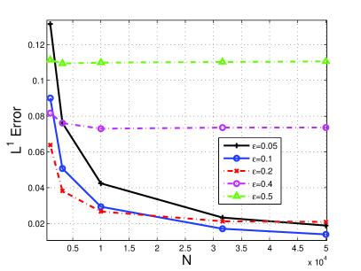
(a) $L^{1}$ error as a function of $N$

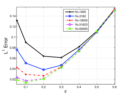
(b) $L^{1}$ error as a function of $\epsilon$

Figure 1: $L^{1}$ error as a function of the number of particles, $N$, (on the left graph) and the mollifier window width, $\epsilon$, (on the right graph), for the Burgers equation (4.1), dimension $d=1$.

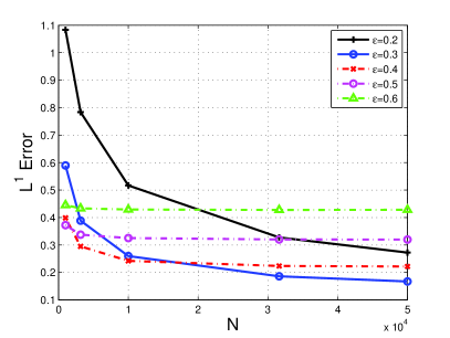
(a) $L^{1}$ error as a function of $N$

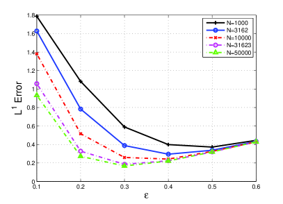
(b) $L^{1}$ error as a function of $\epsilon$

Figure 2: $L^{1}$ error as a function of the number of particles, $N$, (on the left graph) and the mollifier window width, $\epsilon$, (on the right graph), for the KPZ equation (4.7), dimension $d=5$.

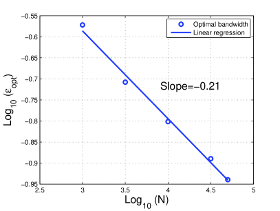
(a) $\varepsilon_{opt}$ as a function of $N$ for Burgers ($d=1$)

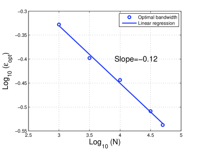
(b) $\varepsilon_{opt}$ as a function of $N$ for KPZ ($d=5$)

Figure 3: Optimal bandwidth, $\varepsilon_{opt}$, as a function of the number of particles, for Burgers equation with $d=1$ (left graph) and for the KPZ equation (4.7) with $d=5$ (right graph).

5 Appendix

Proof of Lemma 3.5.

Let us fix $\varepsilon>0,N\in\mathbb{N}^{\star}$, $t\in[0,T]$. We first recall that for almost all $x\in\mathbb{R}^{d}$,

$$\bar{u}^{\varepsilon,N}_{t}(x)=\frac{1}{N}\sum_{i=1}^{N}K_{\varepsilon}(x-\bar{\xi}^{i}_{t})\bar{V}_{t}\big{(}\bar{\xi}^{i},\bar{u}^{\varepsilon,N}(\bar{\xi}^{i}),\nabla\bar{u}^{\varepsilon,N}(\bar{\xi}^{i})\big{)},$$ (5.1)

for which $\bar{V}_{t}$ is given by (3.10). Let us fix $i\in\{1,\cdots,N\}$.

• Proof of (3.16). We only give details for the proof of the first inequality since the second one can be established through similar arguments.
  From the second line equation of (5.1), we have

  $$|\bar{u}^{\varepsilon,N}_{r(t)}(x)-\bar{u}^{\varepsilon,N}_{r(t)}(y)| \leq \frac{1}{N}\sum_{i=1}^{N}\big{|}K_{\varepsilon}(x-\bar{\xi}^{i}_{r(t)})-K_{\varepsilon}(y-\bar{\xi}^{i}_{r(t)})\big{|}\bar{V}_{r(t)}\big{(}\bar{\xi}^{i},\bar{u}^{\varepsilon,N}(\bar{\xi}^{i}),\nabla\bar{u}^{\varepsilon,N}(\bar{\xi}^{i})\big{)}$$ (5.2)

  $$\leq \frac{e^{M_{\Lambda}T}}{N\varepsilon^{d+1}}\sum_{i=1}^{N}L_{K}|x-y|$$

  $$\leq \frac{e^{M_{\Lambda}T}L_{K}}{\varepsilon^{d+1}}|x-y|\ ,$$

  where for the second step above, we have used the fact that $K$ is in particular Lipschitz. The same arguments lead also to

  $$|\nabla\bar{u}^{\varepsilon,N}_{r(t)}(x)-\nabla\bar{u}^{\varepsilon,N}_{r(t)}(y)| \leq \frac{e^{M_{\Lambda}T}L_{\nabla K}}{\varepsilon^{d+2}}|x-y|\ ,$$ (5.3)

  which ends the proof of (3.16).

• Proof of (3.17). From

  $$\bar{u}^{\varepsilon,N}_{t}(x)={\displaystyle\frac{1}{N}\sum_{i=1}^{N}K_{\varepsilon}(x-\bar{\xi}^{i}_{t})\bar{V}_{t}\big{(}\bar{\xi}^{i},\bar{u}^{\varepsilon,N}(\bar{\xi}^{i}),\nabla\bar{u}^{\varepsilon,N}(\bar{\xi}^{i})\big{)}}\ ,\quad x\in\mathbb{R}^{d}\ ,$$ (5.4)

  we deduce, for almost all $x\in\mathbb{R}^{d}$,

  $$|\bar{u}^{\varepsilon,N}_{t}(x)-\bar{u}^{\varepsilon,N}_{r(t)}(x)| \leq \frac{e^{M_{\Lambda}T}}{N}\sum_{i=1}^{N}\Big{|}K_{\varepsilon}(x-\bar{\xi}^{i}_{t})-K_{\varepsilon}(x-\bar{\xi}^{i}_{r(t)})\Big{|}$$

  $$\;+\;\frac{\|K\|_{\infty}}{N\varepsilon^{d}}\sum_{i=1}^{N}\big{|}\bar{V}_{t}\big{(}\bar{\xi}^{i},\bar{u}^{\varepsilon,N}(\bar{\xi}^{i}),\nabla\bar{u}^{\varepsilon,N}(\bar{\xi}^{i})\big{)}-\bar{V}_{r(t)}\big{(}\bar{\xi}^{i},\bar{u}^{\varepsilon,N}(\bar{\xi}^{i}),\nabla\bar{u}^{\varepsilon,N}(\bar{\xi}^{i})\big{)}\big{|}\ .$$

  Since $K$ is Lipschitz with related constant $L_{K}=\|\nabla K\|_{\infty}$, for almost all $x\in\mathbb{R}^{d}$, we obtain

  $$|\bar{u}^{\varepsilon,N}_{t}(x)-\bar{u}^{\varepsilon,N}_{r(t)}(x)| \leq \frac{L_{K}e^{M_{\Lambda}T}}{N\varepsilon^{d+1}}\sum_{i=1}^{N}|\bar{\xi}^{i}_{t}-\bar{\xi}^{i}_{r(t)}|$$

  $$\;+\;\frac{L_{\Lambda}e^{M_{\Lambda}T}\|K\|_{\infty}}{N\varepsilon^{d}}\sum_{i=1}^{N}\int_{r(t)}^{t}\Lambda(r(s),\bar{\xi}^{i}_{r(s)},\bar{u}^{\varepsilon,N}_{r(s)}(\bar{\xi}^{i}_{r(s)}),\nabla\bar{u}^{\varepsilon,N}_{r(s)}(\bar{\xi}^{i}_{r(s)}))ds\ ,$$

  where the second term in (• ‣ 5) comes from inequality (2.3). Since $\Lambda$ is bounded, by taking the supremum w.r.t. $x$ and the expectation in both sides of inequality above we have

  $$\mathbb{E}\Big{[}\|\bar{u}^{\varepsilon,N}_{t}-\bar{u}^{\varepsilon,N}_{r(t)}\|_{\infty}\Big{]} \leq \frac{L_{K}e^{M_{\Lambda}T}}{N\varepsilon^{d+1}}\sum_{i=1}^{N}\mathbb{E}\Big{[}|\bar{\xi}^{i}_{t}-\bar{\xi}^{i}_{r(t)}|\Big{]}$$ (5.7)

  $$\;+\;\frac{L_{\Lambda}e^{M_{\Lambda}T}\|K\|_{\infty}}{\varepsilon^{d}}M_{\Lambda}\delta t\leq\frac{C\sqrt{\delta t}}{\varepsilon^{d+1}}\ ,$$

  where we have used the fact that $\mathbb{E}\Big{[}|\bar{\xi}^{i}_{s}-\bar{\xi}^{i}_{r(s)}|^{2}\Big{]}\leq C\delta t$, since $\Phi,g$ are bounded.
  The bound of $\mathbb{E}\Big{[}\|\nabla\bar{u}^{\varepsilon,N}_{t}-\nabla\bar{u}^{\varepsilon,N}_{r(t)}\|_{\infty}\Big{]}$ is obtained by proceeding exactly in with the same way as above, starting with

  $$\frac{\partial\bar{u}^{\varepsilon,N}_{t}}{\partial x_{\ell}}(\cdot)={\displaystyle\frac{1}{N\varepsilon}\sum_{i=1}^{N}\frac{\partial K_{\varepsilon}}{\partial x_{\ell}}(\cdot-\bar{\xi}^{i}_{t})\bar{V}_{t}\big{(}\bar{\xi}^{i},\bar{u}^{\varepsilon,N}(\bar{\xi}^{i}),\nabla\bar{u}^{\varepsilon,N}(\bar{\xi}^{i})\big{)}}\ ,l=1,\cdots,d\ ,$$ (5.8)

  instead of (5.4), where $x_{\ell}$ denotes the $\ell$-th coordinate of $x\in\mathbb{R}^{d}$. It follows then

  $$\mathbb{E}\Big{[}\|\nabla\bar{u}^{\varepsilon,N}_{t}-\bar{\nabla}u^{\varepsilon,N}_{r(t)}\|_{\infty}\Big{]} \leq \frac{C\sqrt{\delta t}}{\varepsilon^{d+2}}\ .$$ (5.9)

∎

References

• [1] N. Belaribi, F. Cuvelier, and F. Russo. A probabilistic algorithm approximating solutions of a singular PDE of porous media type. Monte Carlo Methods and Applications, 17(4):317–369, 2011.
• [2] N. Belaribi, F. Cuvelier, and F. Russo. Probabilistic and deterministic algorithms for space multidimensional irregular porous media equation. SPDEs: Analysis and Computations, 1(1):3–62, 2013.
• [3] A. Bensoussan, S.P. Sethi, R. Vickson, and N. Derzko. Stochastic production planning with production constraints. SIAM Journal on Control and Optimization, 22(6):920–935, 1984.
• [4] D. P. Bertsekas and S. E. Shreve. Stochastic optimal control, volume 139 of Mathematics in Science and Engineering. Academic Press, Inc. [Harcourt Brace Jovanovich, Publishers], New York-London, 1978. The discrete time case.
• [5] M. Bossy, L. Fezoui, and S. Piperno. Comparison of a stochastic particle method and a finite volume deterministic method applied to Burgers equation. Monte Carlo Methods Appl., 3(2):113–140, 1997.
• [6] M. Bossy and D. Talay. Convergence rate for the approximation of the limit law of weakly interacting particles: application to the Burgers equation. Ann. Appl. Probab., 6(3):818–861, 1996.
• [7] B. Bouchard and N. Touzi. Discrete-time approximation and Monte Carlo simulation of backward stochastic differential equations. Stochastic Process. Appl., 111:175–206, 2004.
• [8] P. Cheridito, H. M. Soner, N. Touzi, and N. Victoir. Second-order backward stochastic differential equations and fully nonlinear parabolic PDEs. Comm. Pure Appl. Math., 60(7):1081–1110, 2007.
• [9] F. Delarue and S. Menozzi. An interpolated stochastic algorithm for quasi-linear PDEs. Math. Comp., 77(261):125–158 (electronic), 2008.
• [10] E. Gobet, J-P. Lemor, and X. Warin. A regression-based Monte Carlo method to solve backward stochastic differential equations. Ann. Appl. Probab., 15(3):2172–2202, 2005.
• [11] A. G. Gray and A. W. Moore. Nonparametric density estimation: Toward computational tractability. In Proceedings of the 2003 SIAM International Conference on Data Mining, pages 203–211. SIAM, 2003.
• [12] P. Henry-Labordère. Counterparty risk valuation: A marked branching diffusion approach. Available at SSRN: http://ssrn.com/abstract=1995503 or http://dx.doi.org/10.2139/ssrn.1995503, 2012.
• [13] P. Henry-Labordère, N. Oudjane, X. Tan, N. Touzi, and X. Warin. Branching diffusion representation of semilinear pdes and Monte Carlo approximations. Available at http://arxiv.org/pdf/1603.01727v1.pdf, 2016.
• [14] P. Henry-Labordère, X. Tan, and N. Touzi. A numerical algorithm for a class of BSDEs via the branching process. Stochastic Process. Appl., 124(2):1112–1140, 2014.
• [15] B. Jourdain and S. Méléard. Propagation of chaos and fluctuations for a moderate model with smooth initial data. Ann. Inst. H. Poincaré Probab. Statist., 34(6):727–766, 1998.
• [16] P. E. Kloeden and E. Platen. Numerical solution of stochastic differential equations, volume 23 of Applications of Mathematics (New York). Springer-Verlag, Berlin, 1992.
• [17] A. Le Cavil, N. Oudjane, and F. Russo. Particle system algorithm and chaos propagation related to a non-conservative McKean type stochastic differential equations. Stochastics and Partial Differential Equations: Analysis and Computation, pages 1–37, 2016.
• [18] A. Le Cavil, N. Oudjane, and F. Russo. Probabilistic representation of a class of non-conservative nonlinear partial differential equations. ALEA Lat. Am. J. Probab. Math. Stat., 13(2):1189–1233, 2016.
• [19] A. Le Cavil, N. Oudjane, and F. Russo. Forward Feynman-Kac type representation for semilinear nonconservative partial differential equations. Preprint hal-01353757, version 3, 2017.
• [20] E. Pardoux. Backward stochastic differential equations and viscosity solutions of systems of semilinear parabolic and elliptic PDEs of second order. In Stochastic analysis and related topics, VI (Geilo, 1996), volume 42 of Progr. Probab., pages 79–127. Birkhäuser Boston, Boston, MA, 1998.
• [21] É. Pardoux and S. G. Peng. Adapted solution of a backward stochastic differential equation. Systems Control Lett., 14(1):55–61, 1990.
• [22] E. Pardoux and A. Raşcanu. Stochastic differential equations, Backward SDEs, Partial differential equations, volume 69. Springer, 2014.
• [23] B. W. Silverman. Density estimation for statistics and data analysis. Monographs on Statistics and Applied Probability. Chapman & Hall, London, 1986.