Interpretable Graph-Based Semi-Supervised Learning via Flows

Abstract

In this paper, we consider the interpretability of the foundational Laplacian-based semi-supervised learning approaches on graphs. We introduce a novel flow-based learning framework that subsumes the foundational approaches and additionally provides a detailed, transparent, and easily understood expression of the learning process in terms of graph flows. As a result, one can visualize and interactively explore the precise subgraph along which the information from labeled nodes flows to an unlabeled node of interest. Surprisingly, the proposed framework avoids trading accuracy for interpretability, but in fact leads to improved prediction accuracy, which is supported both by theoretical considerations and empirical results. The flow-based framework guarantees the maximum principle by construction and can handle directed graphs in an out-of-the-box manner.

1 Introduction

Classification and regression problems on networks and data clouds can often benefit from leveraging the underlying connectivity structure. One way of taking advantage of connectivity is provided by graph-based semi-supervised learning approaches, whereby the labels, or values, known on a subset of nodes, are propagated to the rest of the graph. Laplacian-based approaches such as Harmonic Functions (?) and Laplacian Regularization (?) epitomize this class of methods. Although a variety of improvements and extensions have been proposed (?; ?; ?; ?; ?), the interpretability of these learning algorithms has not received much attention and remains limited to the analysis of the obtained prediction weights. In order to promote accountability and trust, it is desirable to have a more transparent representation of the prediction process that can be visualized, interactively examined, and thoroughly understood.

Despite the label propagation intuition behind these algorithms, devising interpretable versions of Harmonic Functions (HF) or Laplacian Regularization (LR) is challenging for a number of reasons. First, since these algorithms operate on graphs in a global manner, any interactive examination of the prediction process would require visualizing the underlying graph, which becomes too complex for even moderately sized graphs. Second, we do not have the luxury of trading prediction accuracy for interpretability: HF/LR have been superseded by newer methods and we cannot afford falling too far behind the current state of the art in terms of the prediction accuracy. Finally, HF and LR possess useful properties such as linearity and maximum principle that are worth preserving.

In this paper, we introduce a novel flow-based semi-supervised learning framework that subsumes HF and LR as special cases, and overcomes all of these challenges. The key idea is to set up a flow optimization problem for each unlabeled node, whereby the flow sources are the labeled nodes, and there is a single flow destination—the unlabeled node under consideration. The source nodes can produce as much out-flow as needed; the destination node requires a unit in-flow. Under these constraints, the flow optimizing a certain objective is computed, and the amount of flow drawn from each of the labeled nodes gives the prediction weights. The objective function contains an $\ell_{1}$-norm like term, whose strength allows controlling the sparsity of the flow and, as a result, its spread over the graph. When this term is dropped, we prove that this scheme can be made equivalent to either the HF or LR method.

This approach was chosen for several reasons. First, the language of flows provides a detailed, transparent, and easily understood expression of the learning process which facilitates accountability and trust. Second, the sparsity term results in flows that concentrate on smaller subgraphs; additionally, the flows induce directionality on these subgraphs. Smaller size and directedness allow using more intuitive graph layouts (?). As a result, one can visualize and interactively explore the precise subgraph along which the information from labeled nodes flows to an unlabeled node of interest. Third, the sparsity term injects locality into prediction weights, which helps to avoid flat, unstable solutions observed with pure HF/LR in high-dimensional settings (?). Thus, not only do we avoid trading accuracy for interpretability, but in fact we gain in terms of the prediction accuracy. Fourth, by construction, the flow-based framework is linear and results in solutions that obey the maximum principle, guaranteeing that the predicted values will stay within the range of the provided training values. Finally, directed graphs are handled out-of-the-box and different weights for forward and backward versions of an edge are allowed.

The main contribution of this paper is the proposed flow-based framework (Section 2). We investigate the theoretical properties of the resulting prediction scheme (Section 3) and introduce its extensions (Section 4). After providing computational algorithms that effectively make use of the shared structure in the involved flow optimization problems (Section 5), we present an empirical evaluation both on synthetic and real data (Section 6).

2 Flow-based Framework

We consider the transductive classification/regression problem formulated on a graph $G=(V,E)$ with node-set $V=\{1,2,...,n\}$ and edge-set $E=\{1,2,...,m\}$. A function $f(\cdot)$ known on a subset of labeled nodes $1,2,...,n_{l}$ needs to be propagated to the unlabeled nodes $n_{l}+1,n_{l}+2,...,n$. We concentrate on approaches where the predicted values depend linearly on the values at labeled nodes. Such linearity immediately implies that the predicted value at an unlabeled node $s$ is given by

$$f(s)=\sum_{i=1}^{n_{l}}w_{i}(s)f(i),$$ (1)

where for each $i=1,2,...,n_{l}$, the weight $w_{i}(\cdot)$ captures the contribution of the labeled node $i$.

In this section, we assume that the underlying graph is undirected, and that the edges $e\in E$ of the graph are decorated with dissimilarities $d_{e}>0$, whose precise form will be discussed later. For an unlabeled node $s$, our goal is to compute the weights $w_{i}(s),i=1,2,...,n_{l}$. To this end, we set up a flow optimization problem whereby the flow sources are the labeled nodes, and there is a single flow destination: the node $s$. The source nodes can produce as much out-flow as needed; the sink node $s$ requires a unit in-flow. Under these constraints, the flow optimizing a certain objective function is computed, and the amount of flow drawn from each of the source nodes $i=1,2,...,n_{l}$ gives us the desired prediction weights $w_{i}(s)$.

With these preliminaries in mind, we next write out the flow optimization problem formally. We first arbitrarily orient each edge of the undirected graph, and let $A$ be $n\times m$ signed incidence matrix of the resulting directed graph: for edge $e$, from node $i$ to node $j$, we have $A_{ie}=+1$ and $A_{je}=-1$. This matrix will be useful for formulating the flow conservation constraint. Note that the flow conservation holds at unlabeled nodes, so we will partition $A$ into two blocks. Rows $1...n_{l}$ of $A$ will constitute the $n_{l}\times m$ matrix $A_{l}$ and the remaining rows make up $A_{u}$; these sub-matrices correspond to labeled and unlabeled nodes respectively. The right hand side for the conservation constraints is captured by the $(n-n_{l})\times 1$ column-vector $\mathbf{b}_{s}$ whose entries correspond to unlabeled nodes. All entries of $\mathbf{b}_{s}$ are zero except the $s$-th entry which is set to $-1$, capturing the fact that there is a unit in-flow at the sink node $s$. For each edge $e$, let the sought flow along that edge be $x_{e}$, and let $\mathbf{x}$ be the column-vector with $e$-th entry equal to $x_{e}$. Our flow optimization problem is formulated as:

$$\min_{\mathbf{x}\in\mathbb{R}^{m}}\frac{1}{2}\sum_{e=1}^{m}d_{e}(x_{e}^{2}+\lambda|x_{e}|)\quad\mbox{subject to}\;A_{u}\mathbf{x}=\mathbf{b}_{s},$$ (2)

where $\lambda\geq 0$ is a trade-off parameter.

The prediction weight $w_{i}(s)$ is given by the flow amount drawn from the labeled node $i$. More precisely, the weight vector is computed as $\mathbf{w}(s)=A_{l}\mathbf{x}$ for the optimal $\mathbf{x}$. Note that the optimization problem is strictly convex and, as a result, has a unique solution. Furthermore, the optimization problem must be solved separately for each unlabeled $s$, i.e. for all different vectors $\mathbf{b}_{s}$, and the predicted value at node $s$ is computed via $f(s)=\sum_{i=1}^{n_{l}}w_{i}(s)f(i)=(\mathbf{w}(s))^{\mkern-1.5mu\mathsf{T}}\mathbf{f}_{l}.$

Flow Subgraphs

Our optimization problem resembles that of elastic nets (?), and the $\ell_{1}$-norm like first-order term makes the solution sparse. For a given value of $\lambda,$ taking the optimal flow’s support—all edges that have non-zero flow values and nodes incident to these edges—we obtain a subgraph $G_{s}(\lambda)$ along which the flows get propagated to the node $s$. This subgraph together with the flow values on the edges constitutes an expressive summary of the learning process, and can be analyzed or visualized for further analysis. Potentially, further insights can be obtained by considering $G_{s}(\lambda)$ for different values of $\lambda$ whereby one gets a “regularization path” of flow subgraphs.

In addition, the optimal flow induces directionality on $G_{s}(\lambda)$ as follows. While the underlying graph was oriented arbitrarily, we get a preferred orientation on $G_{s}(\lambda)$ by retaining the directionality of the edges with positive flows, and flipping the edges with negative flows; this process completely removes arbitrariness since the edges of $G_{s}(\lambda)$ have non-zero flow values. In addition, this process makes the optimal flow positive on $G_{s}(\lambda)$; it vanishes on the rest of the underlying graph.

Discussion

To understand the main features of the proposed framework, it is instructive to look at the tension between the quadratic and first-order terms in the objective function. While the first-order term tries to concentrate flows along the shortest paths, the quadratic term tries to spread the flow broadly over the graph. This is formalized in Section 3 by considering two limiting cases of the parameter $\lambda$ and showing that our scheme provably reduces to the HF when $\lambda=0$, and to the 1-nearest neighbor prediction when $\lambda\to\infty$. Thanks to the former limiting case, our scheme inherits from HF the advantage of leveraging the community structure of the underlying graph. The latter case injects locality and keeps the spread of the flow under control.

Limiting the spread of the flow is crucially important for interactive exploration. The flow subgraphs $G_{s}(\lambda)$ get smaller with the increasing parameter $\lambda>0$. As a result, these subgraphs, which serve as the summary of the learning process, can be more easily visualized and interactively explored. Another helpful factor is that, with the induced orientation, $G_{s}(\lambda)$ is a directed acyclic graph (DAG); see Section 3 for a proof. The resulting topological ordering gives an overall direction and hierarchical structure to the flow subgraph, rendering it more accessible to a human companion due to the conceptual resemblance with the commonly used flowchart diagrams.

Limiting the spread of the flow seemingly inhibits fully exploiting the connectivity of the underlying graph. Does this lead to a less effective method? Quite surprisingly the complete opposite is true. HF and LR have been known to suffer from flat, unstable solutions in high-dimensional settings (?). An insightful perspective on this phenomenon was provided in (?; ?) which showed that random walks of the type used in Laplacian-based methods spread too thinly over the graph and “get lost in space” and, as a result, carry minimal useful information. Therefore, limiting the spread within our framework can be seen as an antidote to this problem. Indeed, as empirically confirmed in Section 6, in contrast to HF/LR which suffer from almost uniform weights, flow-based weights with $\lambda>0$ concentrate on a sparse subset of labeled nodes and help to avoid the flat, unstable solutions.

3 Theoretical Properties

In this section we prove a number of properties of the proposed framework. We first study its behavior at the limiting cases of $\lambda=0$ and $\lambda\to\infty$. Next, we prove that for all values of the parameter $\lambda$, the subgraphs $G_{s}(\lambda)$ supporting the flow are acyclic and the maximum principle holds.

Limiting Behavior

Introduce the column-vector $\mathbf{d}$ consisting of dissimilarities $d_{e}$, and the diagonal matrix $D=\mathrm{diag}(\mathbf{d})$. It is easy to see that the matrix $L=AD^{-1}A^{\mkern-1.5mu\mathsf{T}}$ is the un-normalized Laplacian of the underlying graph with edge weights (similarities) given by $1/d_{e}$. As usual, the edge weights enter the Laplacian with a negative sign, i.e. for each edge $e=(i,j)$ we have $L_{ij}=-1/d_{ij}$.

Proposition 1.

When $\lambda=0$, the flow-based prediction scheme is equivalent to the Harmonic Functions approach with the Laplacian $L=AD^{-1}A^{\mkern-1.5mu\mathsf{T}}$.

Proof.

The HF method uses the Laplacian matrix $L$ and constructs predictions by optimizing $\min_{\mathbf{f}\in\mathbb{R}^{n}}\sum_{(i,j)\in E}\,-L_{ij}(f_{i}-f_{j})^{2}$ subject to reproducing the values at labeled nodes, $f_{i}=f(i)$ for $i\in\{1,2,...,n_{l}\}$. By considering the partitions of the Laplacian along labeled and unlabeled nodes, we can write the solution of the HF method as $\mathbf{f}_{u}=-L_{uu}^{-1}L_{ul}\mathbf{f}_{l}$, compare to Eq. (5) in (?).

When $\lambda=0$, the flow optimization problem Eq. (2) is quadratic with linear constraints, and so can be carried out in a closed form (see e.g. Section 4.2.5 of (?)). The optimal flow vector is given by $\mathbf{x}=D^{-1}A_{u}^{\mkern-1.5mu\mathsf{T}}(A_{u}D^{-1}A_{u}^{\mkern-1.5mu\mathsf{T}})^{-1}\mathbf{b}_{s}$, and the weights are computed as $\mathbf{w}(s)=A_{l}\mathbf{x}=A_{l}D^{-1}A_{u}^{\mkern-1.5mu\mathsf{T}}(A_{u}D^{-1}A_{u}^{\mkern-1.5mu\mathsf{T}})^{-1}\mathbf{b}_{s}$. When we plug these weights into the prediction formula (1), we obtain the predicted value at $s$ as $f(s)=(\mathbf{w}(s))^{\mkern-1.5mu\mathsf{T}}\mathbf{f}_{l}=\mathbf{b}_{s}^{\mkern-1.5mu\mathsf{T}}(A_{u}D^{-1}A_{u}^{\mkern-1.5mu\mathsf{T}})^{-1}A_{u}D^{-1}A_{l}^{\mkern-1.5mu\mathsf{T}}\mathbf{f}_{l}.$ Since $\mathbf{b}_{s}$ is zero except at the position corresponding to $s$ where it is $-1$ (this is the reason for the negative sign below), we can put together the formulas for all separate $s$ into a single expression

$$\mathbf{f}_{u}=-(A_{u}D^{-1}A_{u}^{\mkern-1.5mu\mathsf{T}})^{-1}A_{u}D^{-1}A_{l}^{\mkern-1.5mu\mathsf{T}}\mathbf{f}_{l}.$$

By using the Laplacian $L=AD^{-1}A^{\mkern-1.5mu\mathsf{T}}$ and considering its partitions along labeled and unlabeled nodes, we can re-write the formula as $\mathbf{f}_{u}=-L_{uu}^{-1}L_{ul}\mathbf{f}_{l}$, giving the same solution as the HF method.∎

Remark.

The converse is true as well: for any Laplacian $L$ built using non-negative edge weights (recall that off-diagonal entries of such Laplacians are non-positive), the same predictions as HF can be obtained via our approach at $\lambda=0$ with appropriate costs $d_{e}$. When the Laplacian matrix $L$ is symmetric, this easily follows from Proposition 1 by simply setting $d_{ij}=-1/L_{ij}$ for all $(i,j)\in E$. However, when $L$ is not symmetric (e.g. after Markov normalization), we can still match the HF prediction results by setting $d_{ij}=-2/(L_{ij}+L_{ji})$ for all $(i,j)\in E$. The main observation is that while $L$ may be asymmetric, it can always be symmetrized without inducing any change in the optimization objective of the HF method. Indeed the objective $\sum_{(i,j)\in E}\,-L_{ij}(f_{i}-f_{j})^{2}$ is invariant to setting $L_{ij}\leftarrow(L_{ij}+L_{ji})/2$. Now using Proposition 1, we see that by letting $d_{ij}=-2/(L_{ij}+L_{ji})$, our framework with $\lambda=0$ reproduces the same predictions as the HF method.

Proposition 2.

When one formally sets $\lambda=\infty$, the flow based prediction scheme is equivalent to the 1-nearest neighbor prediction.

Proof.

In this setting, the first-order term dominates the cost, and the flow converges to a unit flow along the shortest path (with respect to costs $d_{e}$) from the closest labeled node, say $i^{*}(p)$, to node $p$. We can then easily see that the resulting prediction weights are all zero, except $w_{i^{*}(p)}(p)=1$. Thus, the prediction scheme (1) becomes equivalent to the 1-nearest neighbor prediction. ∎

Acyclicity of Flow Subgraphs

Recall that the optimal solution induces a preferred orientation on subgraph $G_{s}(\lambda)$; this orientation renders the optimal flow positive on $G_{s}(\lambda)$ and zero on the rest of the underlying graph.

Proposition 3.

For all $\lambda\geq 0$, the oriented flow subgraph $G_{s}(\lambda)$ is acyclic.

Proof.

Suppose that $G_{s}(\lambda)$ has a cycle of the form $k_{1}\rightarrow...\rightarrow k_{r}\to k_{1}$. The optimal flow $\mathbf{x}$ is positive along all of the edges of $G_{s}(\lambda)$, including the edges in this cycle; let $x_{0}>0$ be the smallest of the flow values on the cycle. Let $\mathbf{x}_{\mathrm{sub}}$ be the flow vector corresponding to the flow along this cycle with constant flow value of $x_{0}$. Note that $\mathbf{x}-\mathbf{x}_{\mathrm{sub}}$ is a feasible flow, and it has strictly lower cost than $\mathbf{x}$ because the optimization objective is diminished by a decrease in the components of $\mathbf{x}$. This contradiction proves acyclicity of $G_{s}(\lambda)$. ∎

Maximum Principle

It is well-known that harmonic functions satisfy the maximum principle. Here we provide its derivation in terms of the flows, showing that the maximum principle holds in our framework for all settings of the parameter $\lambda$.

Proposition 4.

For all $\lambda\geq 0$ and for all $s$, we have $\forall i,w_{i}(s)\geq 0$ and $\sum_{i=1}^{n_{l}}w_{i}(s)=1$.

Proof.

Non-negativity of weights holds because a flow having a negative out-flow at a labeled node can be made less costly by removing the corresponding sub-flow. The formal proof is similar to the proof or Proposition 3. First, make the flow non-negative by re-orienting the underlying graph (which was oriented arbitrarily). Now suppose that the optimal solution $\mathbf{x}$ results in $w_{i}(s)<0$ for some $i$, meaning that the labeled node $i$ has an in-flow of magnitude $|w_{i}(s)|$. Since all of the flow originates from labeled nodes, there must exist $j\in\{1,...,n_{l}\}/\{i\}$ and a flow-path $j\rightarrow k_{1}\rightarrow...\rightarrow k_{r}\rightarrow i$ with positive flow values along the path; let $x_{0}>0$ be the smallest of these flow values. Let $\mathbf{x}_{\mathrm{sub}}$ be the flow vector corresponding to the flow along this path with constant flow value of $x_{0}$. Note that $\mathbf{x}-\mathbf{x}_{\mathrm{sub}}$ is a feasible flow, and it has strictly lower cost than $\mathbf{x}$ because the optimization objective is diminished by a decrease in the components of $\mathbf{x}$. This contradiction proves the positivity of weights.

The weights, or equivalently the out-flows from the labeled nodes, add up to $1$ because the destination node absorbs a total of a unit flow. More formally, note that by definition, $\mathbf{1}^{\mkern-1.5mu\mathsf{T}}A=\mathbf{0}$. Splitting this along labeled and unlabeled nodes we get $\mathbf{1}^{\mkern-1.5mu\mathsf{T}}A=\mathbf{1}_{l}^{\mkern-1.5mu\mathsf{T}}A_{l}+\mathbf{1}_{u}^{\mkern-1.5mu\mathsf{T}}A_{u}=\mathbf{0}$. Right-multiplying by $\mathbf{x}$ gives $\mathbf{1}_{l}^{\mkern-1.5mu\mathsf{T}}A_{l}\mathbf{x}+\mathbf{1}_{u}^{\mkern-1.5mu\mathsf{T}}A_{u}\mathbf{x}=\mathbf{1}_{l}^{\mkern-1.5mu\mathsf{T}}\mathbf{w}(s)+\mathbf{1}_{u}^{\mkern-1.5mu\mathsf{T}}\mathbf{b}_{s}=\mathbf{1}_{l}^{\mkern-1.5mu\mathsf{T}}\mathbf{w}(s)-1=0$, or $\sum_{i=1}^{n_{l}}w_{i}(s)=1$ as desired. ∎

This proposition together with Eq. (1) guarantees that the function $f(\cdot)$ obeys the maximum principle.

4 Extensions

LR and Noisy Labels

Laplacian Regularization has the advantage of allowing to train with noisy labels. Here, we discuss modifications needed to reproduce LR via our framework in the limit $\lambda=0$. This strategy allows incorporating noisy training labels into the flow framework for all $\lambda\geq 0$.

Consider the LR objective $\mu^{-1}\sum_{i=1}^{n_{l}}(f_{i}\text{\textendash}f(i))^{2}+\sum_{(i,j)\in E}\,-L_{ij}(f_{i}-f_{j})^{2}$, where $f(i)$ are the provided noisy labels/values and $\mu$ is the strength of Laplacian regularization. In this formulation, we need to learn $f_{i}$ for both labeled and unlabeled nodes. The main observation is that the soft labeling terms $\mu^{-1}(f_{i}\text{\textendash}f(i))^{2}$ can be absorbed into the Laplacian by modifying the data graph. For each labeled node $i\in\{1,2,...,n_{l}\}$, introduce a new anchor node $i^{a}$ with a single edge connecting $i^{a}$ to node $i$ with the weight of $\mu^{-1}/2$ (halving offsets doubling in the regularizer sum). Consider the HF learning on the modified graph, where the labeled nodes are the anchor nodes only—i.e. optimize the HF objective on the modified graph with hard constraints $f_{i^{a}}=f(i)$; clearly, this is equivalent to LR. Given the relationship between HF and the flow formulation, this modification results in a flow formulation of LR at the limiting case of $\lambda=0$.

Directed Graphs

Being based on flows, our framework can treat directed graphs very naturally. Indeed, since the flow can only go along the edge direction, we have a new constraint $x_{e}\geq 0$, giving the optimization problem:

$$\min_{\mathbf{x}\in\mathbb{R}_{+}^{m}}\frac{1}{2}\sum_{e=1}^{m}d_{e}(x_{e}^{2}+\lambda x_{e})\quad\mbox{subject to}\;A_{u}\mathbf{x}=\mathbf{b}_{s},$$ (3)

Even when $\lambda=0$, this scheme is novel—due to the non-negativity constraint the equivalence to HF no longer holds. The naturalness of our formulation is remarkable when compared to the existing approaches to directed graphs that use different graph normalizations (?; ?), co-linkage analysis (?), or asymmetric dissimilarity measures (?).

This formulation can also handle graphs with asymmetric weights. Namely, one may have different costs for going forward and backward: the cost of the edge $i\rightarrow j$ can differ from that of $j\rightarrow i$. If needed, such cost differentiation can be applied to undirected graphs by doubling each edge into forward and backward versions. In addition, it may be useful to add opposing edges (with higher costs) into directed graphs to make sure that the flow problem is feasible even if the underlying graph is not strongly connected.

5 Computation

The flow optimization problems discussed in Section 4 can be solved by the existing general convex or convex quadratic solvers. However, general purpose solvers cannot use the shared structure of the problem—namely that everything except the vector $\mathbf{b}_{s}$ is fixed. Here, we propose solvers based on the Alternating Direction Method of Multipliers (ADMM) (?) that allow caching the Cholesky factorization of a relevant matrix and reusing it in all of the iterations for all unlabeled nodes. We concentrate on the undirected version because of the space limitations.

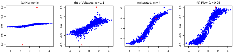
Figure 1: $f(\cdot)$ for a mixture of two Gaussians in $\mathbb{R}^{10}$ for a number of methods.

In the ADMM form, the problem (2) can be written as

$$\min_{\mathbf{x},\mathbf{z}\in\mathbb{R}^{m}}\;\, g(\mathbf{x})+\frac{1}{2}\sum_{e\in E}d_{e}x_{e}^{2}+\lambda\sum_{e\in E}d_{e}|z_{e}|$$

subj to $$\mathbf{x}-\mathbf{z}=\mathbf{0},$$

where $g(x)$ is the $0/\infty$ indicator function of the set $\{\mathbf{x}|A_{u}\mathbf{x}=\mathbf{b}_{s}\}$. Stacking the dissimilarities $d_{e}$ into a column-vector d, and defining the diagonal matrix $D=\mathrm{diag}(\mathbf{d})$, the ADMM algorithm then consists of iterations:

$$\mathbf{x}^{k+1}:= \arg\min_{\mathbf{x}}\>g(\mathbf{x})+\frac{1}{2}\mathbf{x}^{\mkern-1.5mu\mathsf{T}}D\mathbf{x}+\frac{\rho}{2}\|\mathbf{x}-\mathbf{z}^{k}+\mathbf{u}^{k}\|_{2}^{2}$$

$$\mathbf{z}^{k+1}:= S_{\mathbf{d}\lambda/\rho}(\mathbf{x}^{k+1}+\mathbf{u}^{k})$$

$$\mathbf{u}^{k+1}:= \mathbf{u}^{k}+\mathbf{x}^{k+1}-\mathbf{z}^{k+1}$$

Here, $S_{\mathbf{a}}(\mathbf{b})=(\mathbf{b}-\mathbf{a})_{+}-(-\mathbf{b}-\mathbf{a})_{+}$ is the component-wise soft-thresholding function.

The $\mathbf{x}$-iteration can be computed in a closed form as the solution of an equality constrained quadratic program, cf. Section 4.2.5 of (?). Letting $M=\mathrm{diag}(1/(\rho+\mathbf{d}))$, we first solve the linear system $A_{u}MA_{u}^{\mkern-1.5mu\mathsf{T}}\mathbf{y}=2\rho A_{u}M(\mathbf{z}^{k}-\mathbf{u}^{k})-\mathbf{b}_{s}$ for $\mathbf{y}$, and then let $\mathbf{x}^{k+1}:=2\rho M(\mathbf{z}^{k}-\mathbf{u}^{k})-MA_{u}^{\mathsf{T}}\mathbf{y}$. The most expensive step is the involved linear solve. Fortunately, the matrix $A_{u}MA_{u}^{\mkern-1.5mu\mathsf{T}}$ is both sparse (same fill as the graph Laplacian) and positive-definite. Thus, we compute its Cholesky factorization and use it throughout all iterations and for all unlabeled nodes, since $A_{u}MA_{u}^{\mkern-1.5mu\mathsf{T}}$ contains only fixed quantities.

We initialize the iterations by setting $\mathbf{z}^{0}=\mathbf{u}^{0}=\mathbf{0}$, and declare convergence when both $\max(\mathbf{x}^{k+1}-\mathbf{z}^{k+1})$ and $\max(\mathbf{z}^{k+1}-\mathbf{z}^{k})$ fall below a pre-set threshold. As explained in Section 3.3 of (?), these quantities are related to primal and dual feasibilities. Upon convergence, the prediction weights are computed using the formula $\mathbf{w}(s)=A_{l}\mathbf{z}$; thanks to soft-thresholding, using $\mathbf{z}$ instead of $\mathbf{x}$ avoids having a multitude of negligible non-zero entries.

6 Experiments

In this section, we validate the proposed framework and then showcase its interpretability aspect.

6.1 Validation

We experimentally validate a number of claims made about the flow based approach: 1) limiting the spread of the flow via sparsity term results in improved behavior in high-dimensional settings; 2) this improved behavior holds for real-world data sets and leads to increased predictive accuracy over HF; 3) our approach does not fall far behind the state-of-the-art in terms of accuracy. We also exemplify the directed/asymmetric formulation on a synthetic example.

We compare the flow framework to the original HF formulation and also to two improvements of HF designed to overcome the problems encountered in high-dimensional settings: $p$-Voltages—the method advocated in Alamgir and von Luxburg (?) (they call it $q$-Laplacian regularization) and further studied in (?; ?); Iterated Laplacians—a state-of-the-art method proposed in (?).

For data clouds we construct the underlying graph as a weighted $20$-nearest neighbor graph. The edge weights are computed using Gaussian RBF with $\sigma$ set as one-third of the mean distance between a point and its tenth nearest neighbor (?). The normalized graph Laplacian $L$ is used for HF and Iterated Laplacian methods. The edge costs for the flow approach are set by $d_{ij}=-2/(L_{ij}+L_{ji})$ as described in Section 3. The weights for $p$-Voltages are computed as $d_{ij}^{-1/(p-1)}$, see (?; ?).

Mixture of Two Gaussians

Consider a mixture of two Gaussians in $10$-dimensional Euclidean space, constructed as follows. We sample $500$ points from each of the two Gaussians with $\mathbf{\mu}_{1}=\mathbf{\mu}_{2}=\mathbf{0}$ and $\Sigma_{1}=\Sigma_{2}=I$. The points from each Gaussian are respectively shifted by $-1.5$ and $+1.5$ units along the first dimension. A single labeled point is used for each Gaussian; the labels are $-1$ for the left Gaussian and $+1$ for the right one. According to (?; ?), an appropriate value of $p$ for $p$-Voltages is $(10+1)/10=1.1$.

In Figure 1, we plot the estimated functions $f$ for various methods. The sampled points are projected along the first dimension, giving the $x$-axis in these plots; the $y$-axis shows the estimator $f$. Figure 1 (a) confirms the flatness of the HF solution as noted in (?). In classification problems flatness is undesirable as the solution can be easily shifted by a few random labeled samples to favor one or the other class. For regression problems, the estimator $f$ is unsuitable as it fails to be smooth, which can be seen by the discrepancy between the values at labeled nodes (shown as red triangles) and their surrounding.

The $p$-Voltages solution, Figure 1 (b), avoids the instability issue, but is not completely satisfactory in terms of smoothness. The iterated Laplacian and flow methods, Figure 1 (c,d), suffer neither from flatness nor instability. Note that in contrast to iterated Laplacian method, the flow formulation satisfies the maximum principle, and $f$ stays in the range $[-1,1]$ established by the provided labels.

Dataset	Harmonic	p-Voltages	Iterated	Flow
MNIST 3vs8	$8.5\pm 2.4$	$7.8\pm 1.8$	$6.1\pm 2.3$	$6.2\pm 1.6$
MNIST 4vs9	$22.3\pm 8.2$	$13.3\pm 2.8$	$8.5\pm 2.0$	$9.6\pm 2.7$
AUT-AVN	$27.9\pm 13.7$	$19.0\pm 5.1$	$11.5\pm 2.0$	$14.6\pm 2.7$
CCAT	$33.3\pm 8.5$	$25.4\pm 3.5$	$21.5\pm 3.4$	$22.3\pm 3.2$
GCAT	$20.0\pm 11.6$	$13.6\pm 3.7$	$9.2\pm 2.6$	$10.0\pm 1.7$
PCMAC	$30.6\pm 11.2$	$21.4\pm 3.2$	$14.1\pm 1.6$	$18.2\pm 3.3$
REAL-SIM	$31.5\pm 12.1$	$22.4\pm 3.6$	$15.3\pm 2.8$	$17.6\pm 3.3$

Table 1: Misclassification rates (%) and standard deviations.

Dataset	Harmonic	$\lambda=0.025$	$\lambda=0.05$	$\lambda=0.1$	$\lambda=0.2$
MNIST 3vs8	$8.5\pm 2.4$	$5.8\pm 1.6$	$5.9\pm 1.5$	$6.2\pm 1.4$	$6.7\pm 1.4$
MNIST 4vs9	$22.3\pm 8.2$	$9.4\pm 2.8$	$9.3\pm 2.7$	$9.7\pm 2.7$	$10.3\pm 2.7$
AUT-AVN	$27.9\pm 13.7$	$14.0\pm 2.6$	$14.8\pm 2.4$	$16.3\pm 2.3$	$18.4\pm 2.4$
CCAT	$33.3\pm 8.5$	$21.9\pm 3.0$	$22.5\pm 2.8$	$23.2\pm 2.5$	$24.5\pm 2.5$
GCAT	$20.0\pm 11.6$	$9.9\pm 1.6$	$10.8\pm 1.6$	$12.4\pm 1.8$	$14.1\pm 1.7$
PCMAC	$30.6\pm 11.2$	$17.2\pm 2.9$	$18.0\pm 2.5$	$19.5\pm 2.2$	$21.0\pm 2.2$
REAL-SIM	$31.5\pm 12.1$	$17.1\pm 3.4$	$17.7\pm 3.0$	$19.1\pm 2.7$	$21.1\pm 2.4$

Table 2: Misclassification rates (%) and standard deviations.

Benchmark Data Sets

Next we test the proposed method on high-dimensional image and text datasets used in (?), including MNIST 3vs8, MNIST 4vs9, aut-avn, ccat, gcat, pcmac, and real-sim. For each of these, we use a balanced subset of $1000$ samples. In each run we use $n_{l}=50$ labeled samples; in addition, we withheld $50$ samples for validation. The misclassification rate is computed for the remaining 900 samples. The results are averaged over $20$ runs. For $p$-Voltages, the value of $p$ for each run is chosen from $\{1.0625,1.125,1.25,1.5,2\}$ using the best performing value on the validation samples; note that $p=2$ corresponds to HF. For iterated Laplacian method, $m$ is chosen from $\{1,2,4,8,16\}$ with $m=1$ being equivalent to HF. For the flow approach, the value of $\lambda$ is chosen from $\{0,0.025,0.05,0.1,0.2\}$, where $\lambda=0$ is equivalent to HF.

The results summarized in Table 1 show that the flow approach outperforms HF and $p$-Voltages, even with the added benefit of interpretability (which the other methods do not have). The flow approach does have slightly lower accuracy than the state-of-the-art iterated Laplacian method, but we believe that this difference is a tolerable tradeoff for applications where interpretability is required.

Next, we compare HF and the flow approach but this time instead of selecting $\lambda$ by validation we use fixed values. The results presented in Table 2 demonstrate that the flow approach for each of the considered values consistently outperforms the base case of HF (i.e. $\lambda=0$). Note that larger values of $\lambda$ lead to increased misclassification rate, but the change is not drastic. This is important for interactive exploration because larger $\lambda$ values produce smaller flow subgraphs $G_{s}(\lambda)$ that are easier for the human companion to grasp.

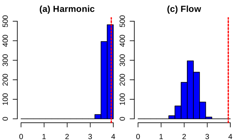
Figure 2: Weight statistics for MNIST 3vs8.

Finally, we show that the improvement over HF observed in these experiments relates to the flatness issue and, therefore, is brought about by limiting the spread of the flow. By analyzing the prediction weights in Eq. (1), we can compare HF to the flow based approach in terms of the flatness of solutions. To focus our discussion, let us concentrate on a single run of MNIST 3vs8 classification problem. Since the weights for the flow based and HF approaches lend themselves to a probabilistic interpretation (by Proposition 4, they are non-negative and add up to $1$), we can look at the entropies of the weights, $H(s)=-\sum_{i}w_{i}(s)\log w_{i}(s)$ for every unlabeled node $s=n_{l}+1,...,n$. For a given unlabeled $s$, the maximum entropy is achieved for uniform weights: $\forall i,w_{i}(s)=1/n_{l}$. Figure 2 shows the histograms of entropies, together with the red vertical line corresponding to the maximum possible entropy. In contrast to the flow based approach, the entropies from HF method are clustered closely to the red line, demonstrating that there is little variation in HF weights, which is a manifestation of the flatness issue.

Directed/Asymmetric Graphs

In this synthetic example, we demonstrate the change in the estimated $f(\cdot)$ induced by the use of asymmetric edge costs in the directed formulation given by Eq. (3). The underlying graph represents the road network of Minnesota, with edges showing the major roads and vertices being their intersections. As in the previous example, we pick two nodes (shown as triangles)) and label them with $\pm 1$ and depict the resulting estimator $f(\cdot)$ for the remaining unlabeled nodes using the shown color-coding. In Figure 3 (a), the graph is undirected, i.e. the edge costs are symmetric. In Figure 3 (b), we consider the directed graph obtained by doubling each edge into forward and backward versions. This time the costs for edges going from south to north ($\mbox{lat}_{i}<\mbox{lat}_{j}$) are multiplied by four. The latter setting makes flows originating at the top labeled node cheaper to travel towards south, and therefore shifts the “decision boundary” to the south.

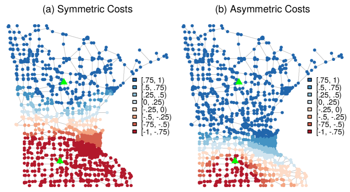
Figure 3: $f(\cdot)$ for symmetric and asymmetric edge costs.

6.2 Interpretability

As stated previously, one of the core benefits of the proposed framework is how it provides a detailed, transparent, and easily understood expression of the learning process. To exemplify this aspect of the proposed framework, we focus our discussion on a fixed data-point $s$ from MNIST 3vs8 and study the corresponding flow subgraphs $G_{s}(\lambda)$ for $\lambda=0.2,0.1$ and $0.05$; see Figure 4 (also see supplementary examples). The digit image for unlabeled node $s$ is outlined in red; the labeled node images are outlined in blue. The flows along the edges are in percents, and have been rounded up to avoid the clutter.

As expected, the size of the subgraph depends on the parameter $\lambda$. Recall that for each $\lambda>0$, the flow optimization automatically selects a subset of edges carrying non-zero flow—this is akin to variable selection in sparse regression (?). The figure confirms that the larger the strength of the sparsity penalty, the fewer edges get selected, and the smaller is the resulting subgraph. The amount of reduction in size is substantial: the underlying graph for this experiment has 1K nodes and ~15K edges.

As claimed, the acyclicity of the flow subgraphs $G_{s}(\lambda)$ leads to more intuitive layouts. We used the “dot” filter from Graphviz (?; ?) which is targeted towards visualizing hierarchical directed graphs. Since our flow subgraphs are DAGs, the “dot” filter gave satisfactory layouts without any manual tweaking. Indeed, all of the visualizations depicted in Figure 4 provide an overall sense of directionality, here from top to bottom: due to acyclicity there are no edges going “backward”. This makes it easy to trace the flow from sources, the labeled nodes, to the sink, the unlabeled node $s$.

Of course, the visualizations in Figure 4 benefit from the fact that the data points are digits, which allows including their images in lieu of abstract graph nodes. The same approach could be used for general image data sets as well. For other data types such as text, the nodes could depict some visual summary of the data point, and then provide a more detailed summary upon a mouse hover.

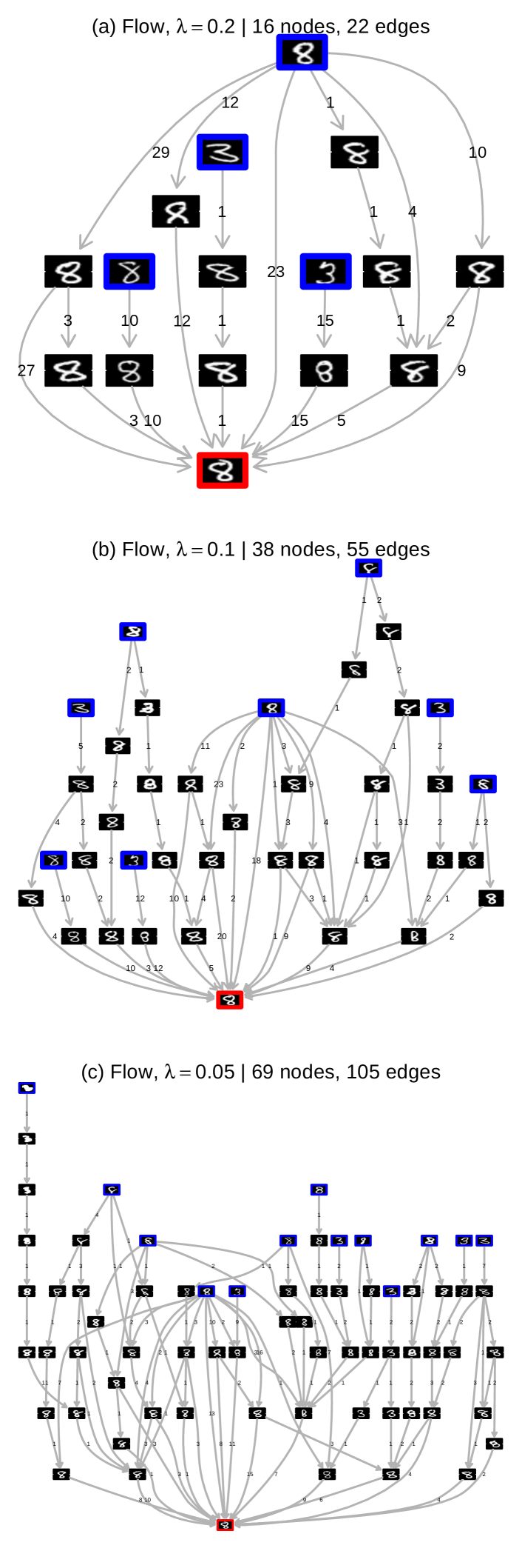
Figure 4: Flow subgraphs $G_{s}(\lambda)$ showing the information propagation from the labeled nodes (outlined in blue) to the unlabeled node $s$ (outlined in red). The flow values on the edges are in percents, and may fail to add up due to rounding.

7 Discussion and Future Work

We have presented a novel framework for graph-based semi-supervised learning that provides a transparent and easily understood expression of the learning process via the language of flows. This facilitates accountability and trust and makes a step towards the goal of improving human-computer collaboration.

Our work is inspired by (?) which pioneered the use of the flow interpretation of the standard resistance distances (c.f. (?)) to introduce a novel class of resistance distances that avoid the pitfalls of the standard resistance distance by concentrating the flow on fewer paths. They also proved an interesting phase transition behavior that led to specific suggestions for Laplacian-based semi-supervised learning. However, their proposal for semi-supervised learning is not based on flows, but rather on an appropriate setting of the parameter in the $p$-Voltages method (which they call $q$-Laplacian regularization); it was further studied in (?; ?). Although it is already apparent from the experimental results that our proposal is distinct from $p$-Voltages, we stress that there is a fundamental theoretical difference: $p$-Voltages method is non-linear and so cannot be expressed via Eq. (1), except when $p=2$. At a deeper level, these methods regularize the estimated function via its value discrepancies at adjacent nodes, and, therefore, do not directly provide a detailed understanding of how the values propagate along the graph.

One immediate direction for future work is to obtain a flow formulation for the iterated Laplacian method which gave best accuracy on the benchmark data sets. This may seem straightforward to do as iterated Laplacian method basically replaces the Laplacian operator $L$ in the regularizer by its power $L^{m}$. However, the matrix $L^{m}$ contains both positive and negative off-diagonal entries, and so, the corresponding edge costs are no longer positive, which renders the flow interpretation problematic. An indirect manifestation of this issue is the lack of a maximum principle for the iterated Laplacian method. Another complicating factor is that the stencils of $L^{m}$ grow very fast with $m$, e.g. $L^{4}$ is nearly a full matrix in the benchmark examples.

Another interesting future work direction is to explore approaches for generating multiple levels of explanations from the flow graph. For example, main paths of the information flow could be identified via graph summarization techniques and presented as an initial coarse summary, either in pictorial or textual form. As the user drills down on particular pathways, more detailed views could be generated.

Additional avenues for future study include algorithmic improvements and applications in other areas. The locality of the resulting weights can be used to devise faster algorithms that operate directly on an appropriate neighborhood of the given unlabeled node. Studying the sparsity parameter $\lambda$ for phase transition behavior can provide guidance for its optimal choice. In another direction, since the flow-based weights are non-negative and add up to 1, they are suitable for semi-supervised learning of probability distributions (?). Finally, the flow-based weights can be useful in different areas, such as descriptor based graph matching or shape correspondence in computer vision and graphics.

Acknowledgments:

We thank Eleftherios Koutsofios for providing expertise on graph visualization and helping with Graphviz. We are grateful to Simon Urbanek for computational support, and Cheuk Yiu Ip and Lauro Lins for help with generating visualizations in R.

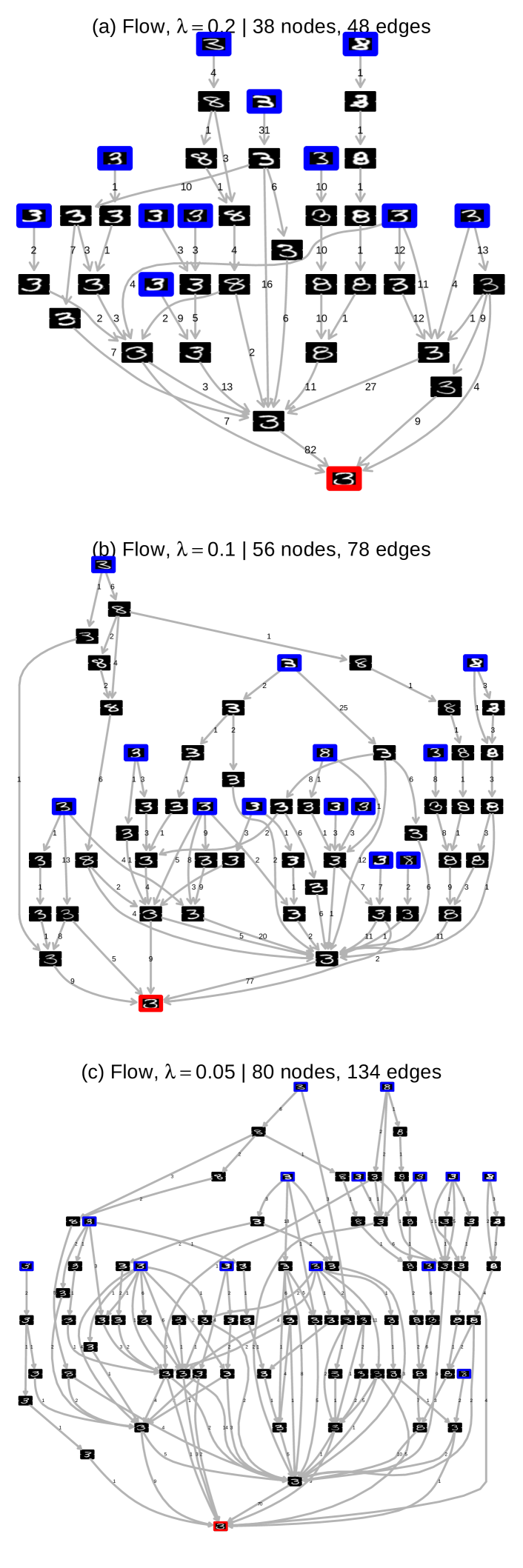
Figure 5: Supplementary example 1

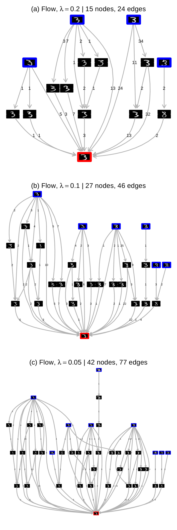
Figure 6: Supplementary example 2

Figure 7: Supplementary example 3

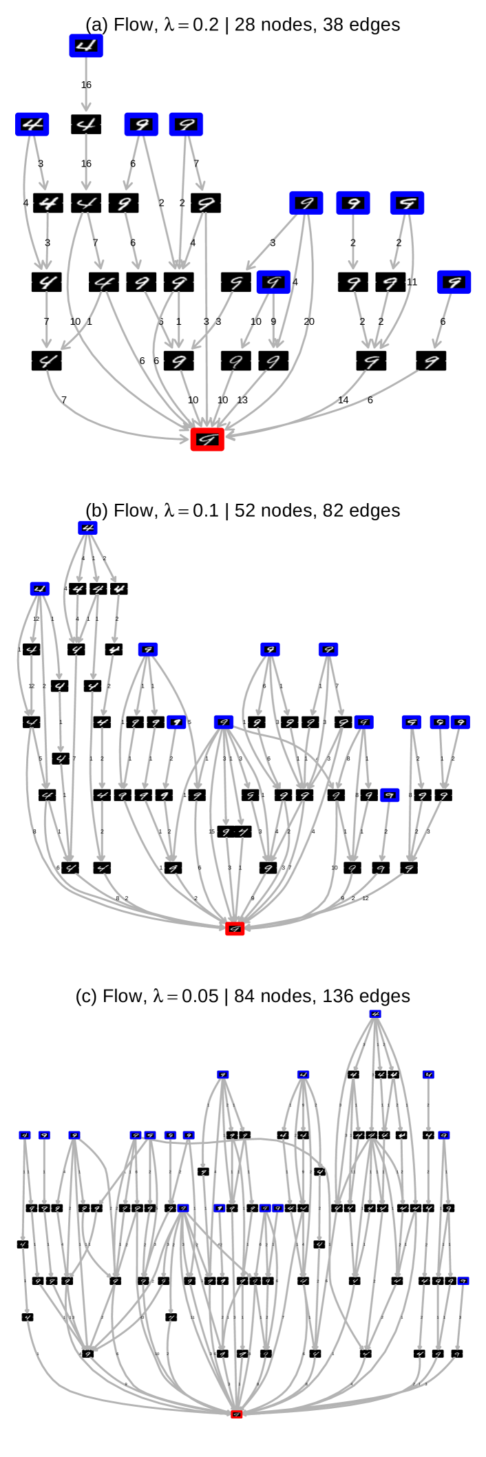
Figure 8: Supplementary example 4

References

- [Alamgir and von Luxburg 2011] Alamgir, M., and von Luxburg, U. 2011. Phase transition in the family of p-resistances. In Advances in Neural Information Processing Systems 24, 379–387.
- [Alaoui et al. 2016] Alaoui, A. E.; Cheng, X.; Ramdas, A.; Wainwright, M. J.; and Jordan, M. I. 2016. Asymptotic behavior of -based Laplacian regularization in semi-supervised learning. In COLT, 879–906.
- [Belkin, Niyogi, and Sindhwani 2006] Belkin, M.; Niyogi, P.; and Sindhwani, V. 2006. Manifold regularization: A geometric framework for learning from labeled and unlabeled examples. JMLR 7:2399–2434.
- [Bollobas 1998] Bollobas, B. 1998. Modern Graph Theory. Graduate texts in mathematics. Heidelberg: Springer.
- [Boyd et al. 2011] Boyd, S. P.; Parikh, N.; Chu, E.; Peleato, B.; and Eckstein, J. 2011. Distributed optimization and statistical learning via the alternating direction method of multipliers. Foundations and Trends in Machine Learning 3(1):1–122.
- [Bridle and Zhu 2013] Bridle, N., and Zhu, X. 2013. -voltages: Laplacian regularization for semi-supervised learning on high-dimensional data. Eleventh Workshop on Mining and Learning with Graphs (MLG2013).
- [Chapelle, Schölkopf, and Zien 2006] Chapelle, O.; Schölkopf, B.; and Zien, A., eds. 2006. Semi-Supervised Learning. Cambridge, MA: MIT Press.
- [Gansner and North 2000] Gansner, E. R., and North, S. C. 2000. An open graph visualization system and its applications to software engineering. Softw. Pract. Exper. 30(11):1203–1233.
- [Gansner et al. 1993] Gansner, E. R.; Koutsofios, E.; North, S. C.; and Vo, K.-P. 1993. A technique for drawing directed graphs. IEEE Trans. Softw. Eng. 19(3):214–230.
- [Hastie, Tibshirani, and Friedman 2009] Hastie, T. J.; Tibshirani, R. J.; and Friedman, J. H. 2009. The elements of statistical learning : data mining, inference, and prediction. Springer series in statistics. New York: Springer.
- [Nadler, Srebro, and Zhou 2009] Nadler, B.; Srebro, N.; and Zhou, X. 2009. Statistical analysis of semi-supervised learning: The limit of infinite unlabelled data. In Advances in Neural Information Processing Systems 22. 1330–1338.
- [Solomon et al. 2014] Solomon, J.; Rustamov, R.; Leonidas, G.; and Butscher, A. 2014. Wasserstein propagation for semi-supervised learning. In Proceedings of the 31st International Conference on Machine Learning (ICML-14), 306–314.
- [Subramanya and Bilmes 2011] Subramanya, A., and Bilmes, J. 2011. Semi-supervised learning with measure propagation. JMLR 12:3311–3370.
- [von Luxburg, Radl, and Hein 2010] von Luxburg, U.; Radl, A.; and Hein, M. 2010. Getting lost in space: Large sample analysis of the resistance distance. In Lafferty, J. D.; Williams, C. K. I.; Shawe-Taylor, J.; Zemel, R. S.; and Culotta, A., eds., Advances in Neural Information Processing Systems 23. 2622–2630.
- [von Luxburg, Radl, and Hein 2014] von Luxburg, U.; Radl, A.; and Hein, M. 2014. Hitting and commute times in large random neighborhood graphs. Journal of Machine Learning Research 15(1):1751–1798.
- [Wang, Ding, and Huang 2010] Wang, H.; Ding, C.; and Huang, H. 2010. Directed graph learning via high-order co-linkage analysis. ECML PKDD’10, 451–466.
- [Wu et al. 2012] Wu, X.; Li, Z.; So, A. M.; Wright, J.; and Chang, S. 2012. Learning with partially absorbing random walks. In Advances in Neural Information Processing Systems 25. 3086–3094.
- [Zhou and Belkin 2011] Zhou, X., and Belkin, M. 2011. Semi-supervised learning by higher order regularization. ICML 15:892–900.
- [Zhou, Huang, and Schölkopf 2005] Zhou, D.; Huang, J.; and Schölkopf, B. 2005. Learning from labeled and unlabeled data on a directed graph. In ICML, 1036–1043.
- [Zhou, Schölkopf, and Hofmann 2004] Zhou, D.; Schölkopf, B.; and Hofmann, T. 2004. Semi-supervised learning on directed graphs. In Advances in Neural Information Processing Systems 17, 1633–1640.
- [Zhu, Ghahramani, and Lafferty 2003] Zhu, X.; Ghahramani, Z.; and Lafferty, J. D. 2003. Semi-supervised learning using Gaussian fields and harmonic functions. In ICML, 912–919.
- [Zhu 2008] Zhu, X. 2008. Semi-supervised learning literature survey. Technical Report 1530, Computer Sciences, University of Wisconsin-Madison.