Heuristics with Performance Guarantees for the Minimum Number of Matches Problem in Heat Recovery Network Design

Abstract

Heat exchanger network synthesis exploits excess heat by integrating process hot and cold streams and improves energy efficiency by reducing utility usage. Determining provably good solutions to the minimum number of matches is a bottleneck of designing a heat recovery network using the sequential method. This subproblem is an $\mathcal{NP}$-hard mixed-integer linear program exhibiting combinatorial explosion in the possible hot and cold stream configurations. We explore this challenging optimization problem from a graph theoretic perspective and correlate it with other special optimization problems such as cost flow network and packing problems. In the case of a single temperature interval, we develop a new optimization formulation without problematic big-M parameters. We develop heuristic methods with performance guarantees using three approaches: (i) relaxation rounding, (ii) water filling, and (iii) greedy packing. Numerical results from a collection of 51 instances substantiate the strength of the methods.

This manuscript is dedicated, with deepest respect, to the memory of Professor C. A. Floudas. Professor Floudas showed that, given many provably-strong solutions to the minimum number of matches problem, he could design effective heat recovery networks. So the diverse solutions generated by this manuscript directly improve Professor Floudas’ method for automatically generating heat exchanger network configurations.

1 Introduction

Heat exchanger network synthesis (HENS) minimizes cost and improves energy recovery in chemical processes (Biegler et al. 1997, Smith 2000, Elia et al. 2010, Baliban et al. 2012). HENS exploits excess heat by integrating process hot and cold streams and improves energy efficiency by reducing utility usage (Floudas and Grossmann 1987, Gundersen and Naess 1988, Furman and Sahinidis 2002, Escobar and Trierweiler 2013). Floudas et al. (2012) review the critical role of heat integration for energy systems producing liquid transportation fuels (Niziolek et al. 2015). Other important applications of HENS include: refrigeration systems (Shelton and Grossmann 1986), batch semi-continuous processes (Zhao et al. 1998, Castro et al. 2015) and water utilization systems (Bagajewicz et al. 2002).

Heat exchanger network design is a mixed-integer nonlinear optimization (MINLP) problem (Yee and Grossmann 1990, Ciric and Floudas 1991, Papalexandri and Pistikopoulos 1994, Hasan et al. 2010). Mistry and Misener (2016) recently showed that expressions incorporating logarithmic mean temperature difference, i.e. the nonlinear nature of heat exchange, may be reformulated to decrease the number of nonconvex nonlinear terms in the optimization problem. But HENS remains a difficult MINLP with many nonconvex nonlinearities. One way to generate good HENS solutions is to use the so-called sequential method (Furman and Sahinidis 2002). The sequential method decomposes the original HENS MINLP into three tasks: (i) minimizing utility cost, (ii) minimizing the number of matches, and (iii) minimizing the investment cost. The method optimizes the three mathematical models sequentially with: (i) a linear program (LP) (Cerda et al. 1983, Papoulias and Grossmann 1983), (ii) a mixed-integer linear program (MILP) (Cerda and Westerberg 1983, Papoulias and Grossmann 1983), and (iii) a nonlinear program (NLP) (Floudas et al. 1986). The sequential method may not return the global solution of the original MINLP, but solutions generated with the sequential method are practically useful.

This paper investigates the minimum number of matches problem (Floudas 1995), the computational bottleneck of the sequential method. The minimum number of matches problem is a strongly $\mathcal{NP}$-hard MILP (Furman and Sahinidis 2001). Mathematical symmetry in the problem structure combinatorially increases the possible stream configurations and deteriorates the performance of exact, tree-based algorithms (Kouyialis and Misener 2017).

Because state-of-the-art approaches cannot solve the minimum number of matches problem to global optimality for moderately-sized instances (Chen et al. 2015b), engineers develop experience-motivated heuristics (Linnhoff and Hindmarsh 1983, Cerda et al. 1983). Linnhoff and Hindmarsh (1983) highlight the importance of generating good solutions quickly: a design engineer may want to actively interact with a good minimum number of matches solution and consider changing the utility usage as a result of the MILP outcome. Furman and Sahinidis (2004) propose a collection of approximation algorithms, i.e. heuristics with performance guarantees, for the minimum number of matches problem by exploiting the LP relaxation of an MILP formulation. Furman and Sahinidis (2004) present a unified worst-case analysis of their algorithms’ performance guarantees and show a non-constant approximation ratio scaling with the number of temperature intervals. They also prove a constant performance guarantee for the single temperature interval problem.

The standard MILP formulations for the minimum number of matches contain big-M constraints, i.e. the on/off switches associated with weak continuous relaxations of MILP. Both optimization-based heuristics and exact state-of-the-art methods for solving minimum number of matches problem are highly affected by the big-M parameter. Trivial methods for computing the big-M parameters are typically adopted, but Gundersen et al. (1997) propose a tighter way of computing the big-M parameters.

This manuscript develops new heuristics and provably efficient approximation algorithms for the minimum number of matches problem. These methods have guaranteed solution quality and efficient run-time bounds. In the sequential method, many possible stream configurations are required to evaluate the minimum overall cost (Floudas 1995), so a complementary contribution of this work is a heuristic methodology for producing multiple solutions efficiently. We classify the heuristics based on their algorithmic nature into three categories: (i) relaxation rounding, (ii) water filling, and (iii) greedy packing.

The relaxation rounding heuristics we consider are (i) Fractional LP Rounding (FLPR), (ii) Lagrangian Relaxation Rounding (LRR), and (iii) Covering Relaxation Rounding (CRR). The water-filling heuristics are (i) Water-Filling Greedy (WFG), and (ii) Water-Filling MILP (WFM). Finally, the greedy packing heuristics are (i) Largest Heat Match LP-based (LHM-LP), (ii) Largest Heat Match Greedy (LHM), (iii) Largest Fraction Match (LFM), and (iv) Shortest Stream (SS). Major ingredients of these heuristics are adaptations of single temperature interval algorithms and maximum heat computations with match restrictions. We propose (i) a novel MILP formulation, and (ii) an improved greedy approximation algorithm for the single temperature interval problem. Furthermore, we present (i) a greedy algorithm computing maximum heat between two streams and their corresponding big-M parameter, (ii) an LP computing the maximum heat in a single temperature interval using a subset of matches, and (iii) an extended maximum heat LP using a subset of matches on multiple temperature intervals.

The manuscript proceeds as follows: Section 2 formally defines the minimum number of matches problem and discusses mathematical models. Section 3 discusses computational complexity and introduces a new $\mathcal{NP}$-hardness reduction of the minimum number of matches problem from bin packing. Section 4 focusses on the single temperature interval problem. Section 5 explores computing the maximum heat exchanged between the streams with match restrictions. Sections 6 - 8 present our heuristics for the minimum number of matches problem based on: (i) relaxation rounding, (ii) water filling, and (iii) greedy packing, respectively, as well as new theoretical performance guarantees. Section 9 evaluates experimentally the heuristics and discusses numerical results. Sections 10 and 11 discuss the manuscript contributions and conclude the paper.

2 Minimum Number of Matches for Heat Exchanger Network Synthesis

This section defines the minimum number of matches problem and presents the standard transportation and transshipment MILP models. Table LABEL:tbl:notation contains the notation.

Table 1: Nomenclature

Name	Description
Cardinalities
$n$	Number of hot streams
$m$	Number of cold streams
$k$	Number of temperature intervals
$v$	Number of matches (objective value)
Indices
$i\in H$	Hot stream
$j\in C$	Cold stream
$s,t,u\in T$	Temperature interval
$b\in B$	Bin (single temperature interval problem)
Sets
$H$, $C$	Hot, cold streams
$T$	Temperature intervals
$M$	Set of matches (subset of $H\times C$)
$C_{i}(M),H_{j}(M)$	Cold, hot streams matched with $i\in H$, $j\in C$ in $M$
$B$	Bins (single temperature interval problem)
$A(M)$	Set of valid quadruples $(i,s,j,t)$ with respect to a set $M$ of matches
$A_{u}(M)$	Set of quadruples $(i,s,j,t)\in A(M)$ with $s\leq u<t$
$V^{H}(M)$	Set of pairs $(i,s)\in H\times T$ appearing in $A(M)$ (transportation vertices)
$V^{C}(M)$	Set of pairs $(j,t)\in C\times T$ appearing in $A(M)$ (transportation vertices)
$V_{i,s}^{C}(M)$	Set of pairs $(j,t)\in V^{C}(M)$ such that $(i,s,j,t)$ belongs to $A(M)$
$V_{j,t}^{H}(M)$	Set of pairs $(i,s)\in V^{H}(M)$ such that $(i,s,j,t)$ belongs to $A(M)$
Parameters
$h_{i}$	Total heat supplied by hot stream $i$ ($h_{i}=\sum_{s\in T}\sigma_{i,s}$)
$h_{\max}$	Maximum heat among all hot streams ($h_{\max}=\max_{i\in H}\{h_{i}\}$)
$c_{j}$	Total heat demanded by cold stream $j$ ($c_{j}=\sum_{t\in T}\delta_{j,t}$)
$\sigma_{i,s}$	Heat supply of hot stream $i$ in interval $s$
$\delta_{j,t}$	Heat demand of cold stream $j$ in interval $t$
$\vec{\sigma},\vec{\delta}$	Vectors of all heat supplies, demands
$\vec{\sigma}_{t},\vec{\delta}_{t}$	Vectors of all heat supplies, demands in temperature interval $t$
$R_{t}$	Residual heat exiting temperature interval $t$
$U_{i,j}$	Upper bound (big-M parameter) on the heat exchanged via match $(i,j)$
$\lambda_{i,j}$	Fractional cost approximation of match $(i,j)$ (Lagrangian relaxation)
$\vec{\lambda}$	Vector of all fractional cost approximations $\lambda_{i,j}$
Variables
$y_{i,j}$	Binary variable indicating whether $i$ and $j$ are matched
$q_{i,j,t}$	Heat of hot stream $i$ received by cold stream $j$ in interval $t$
$q_{i,s,j,t}$	Heat exported by hot stream $i$ in $s$ and received by cold stream $j$ in $t$
$\vec{y},\vec{q}$	Vectors of binary, continuous variables
$r_{i,s}$	Heat residual of heat of hot stream $i$ exiting $s$
$x_{b}$	Binary variable indicating whether bin $b$ is used
$w_{i,b}$	Binary variable indicating whether hot stream $i$ is placed in bin $b$
$z_{j,b}$	Binary variable indicating whether cold stream $j$ is placed in bin $b$
Other
$N$	Minimum cost flow network
$G$	Solution graph (single temperature interval problem)
$\phi(M)$	Filling ratio of a set $M$ of matches
$\vec{y}^{f},\vec{q}^{f}$	Optimal fractional solution
$\alpha_{i},\beta_{j}$	Number of matches of hot stream $i$, cold stream $j$
$L_{i,j}$	Heat exchanged from hot stream $i$ to cold stream $j$
$I$	Instance of the problem
$r$	Remaining heat of an algorithm

2.1 Problem Definition

Heat exchanger network design involves a set $HS$ of hot process streams to be cooled and a set $CS$ of cold process streams to be heated. Each hot stream $i$ posits an initial temperature $T_{\text{in},i}^{HS}$ and a target temperature $T_{\text{out},i}^{HS}$ ($<T_{\text{in},i}^{HS}$). Analogously, each cold stream $j$ has an initial temperature $T_{\text{in},j}^{CS}$ and a target temperature $T_{\text{out},j}^{CS}$ ($>T_{\text{in},j}^{CS}$). Every hot stream $i$ and cold stream $j$ are associated flow rate heat capacities $FCp_{i}$ and $FCp_{j}$, respectively. Minimum heat recovery approach temperature $\Delta T_{\min}$ relates the hot and cold stream temperature axes. A hot utility $i$ in a set $HU$ and a cold utility $j$ in a set $CU$ may be purchased at a cost, e.g. with unitary costs $\kappa_{i}^{HU}$ and $\kappa_{j}^{CU}$. Like the streams, the utilities have inlet and outlet temperatures $T_{\text{in},i}^{HU}$, $T_{\text{out},i}^{HU},T_{\text{in},j}^{CU}$ and $T_{\text{out},j}^{CU}$. The first step in a sequential approach to HENS minimizes the utility cost and thereby specifies the heat each utility introduces in the network. The next step minimizes the number of matches. F discusses the transition from the minimizing utility cost to minimizing the number of matches. After this transition, each utility may, without loss of generality, be treated as a stream.

The minimum number of matches problem posits a set of hot process streams to be cooled and a set of cold process streams to be heated. Each stream is associated with an initial and a target temperature. This set of temperatures defines a collection of temperature intervals. Each hot stream exports (or supplies) heat in each temperature interval between its initial and target temperatures. Similarly, each cold stream receives (or demands) heat in each temperature interval between its initial and target temperatures. F formally defines the temperature range partitioning. Heat may flow from a hot to a cold stream in the same or a lower temperature interval, but not in a higher one. In each temperature interval, the residual heat descends to lower temperature intervals. A zero heat residual is a pinch point. A pinch point restricts the maximum energy integration and divides the network into subnetworks.

A problem instance consists of a set $H=\{1,2,\ldots,n\}$ of hot streams, a set $C=\{1,2,\ldots,m\}$ of cold streams, and a set $T=\{1,2,\ldots,k\}$ of temperature intervals. Hot stream $i\in H$ has heat supply $\sigma_{i,s}$ in temperature interval $s\in T$ and cold stream $j\in C$ has heat demand $\delta_{j,t}$ in temperature interval $t\in T$. Heat conservation is satisfied, i.e. $\sum_{i\in H}\sum_{s\in T}\sigma_{i,s}=\sum_{j\in C}\sum_{t\in T}\delta_{j,t}$. We denote by $h_{i}=\sum_{s\in T}\sigma_{i,s}$ the total heat supply of hot stream $i\in H$ and by $c_{j}=\sum_{t\in T}\delta_{j,t}$ the total heat demand of cold stream $j\in C$.

A feasible solution specifies a way to transfer the hot streams’ heat supply to the cold streams, i.e. an amount $q_{i,s,j,t}$ of heat exchanged between hot stream $i\in H$ in temperature interval $s\in T$ and cold stream $j\in C$ in temperature interval $t\in T$. Heat may only flow to the same or a lower temperature interval, i.e. $q_{i,s,j,t}=0$, for each $i\in H$, $j\in C$ and $s,t\in T$ such that $s>t$. A hot stream $i\in H$ and a cold stream $j\in C$ are matched, if there is a positive amount of heat exchanged between them, i.e. $\sum_{s,t\in T}q_{i,s,j,t}>0$. The objective is to find a feasible solution minimizing the number of matches $(i,j)$.

2.2 Mathematical Models

The transportation and transshipment models formulate the minimum number of matches as a mixed-integer linear program (MILP).

Transportation Model (Cerda and Westerberg 1983)

As illustrated in Figure 1(a), the transportation model represents heat as a commodity transported from supply nodes to destination nodes. For each hot stream $i\in H$, there is a set of supply nodes, one for each temperature interval $s\in T$ with $\sigma_{i,s}>0$. For each cold stream $j\in C$, there is a set of demand nodes, one for each temperature interval $t\in T$ with $\delta_{j,t}>0$. There is an arc between the supply node $(i,s)$ and the destination node $(j,t)$ if $s\leq t$, for each $i\in H$, $j\in C$ and $s,t\in T$.

In the MILP formulation, variable $q_{i,s,j,t}$ specifies the heat transferred from hot stream $i\in H$ in temperature interval $s\in T$ to cold stream $j\in C$ in temperature interval $t\in T$. Binary variable $y_{i,j}$ if whether streams $i\in H$ and $j\in C$ are matched or not. Parameter $U_{i,j}$ is a big-M parameter bounding the amount of heat exchanged between every pair of hot stream $i\in H$ and cold stream $j\in C$, e.g. $U_{i,j}=\min\{h_{i},c_{j}\}$. The problem is formulated:

min $$\sum_{i\in H}\sum_{j\in C}y_{i,j}$$ (1)

$$\sum_{j\in C}\sum_{t\in T}q_{i,s,j,t}=\sigma_{i,s} i\in H,s\in T$$ (2)

$$\sum_{i\in H}\sum_{s\in T}q_{i,s,j,t}=\delta_{j,t} j\in C,t\in T$$ (3)

$$\sum_{s,t\in T}q_{i,s,j,t}\leq U_{i,j}\cdot y_{i,j} i\in H,j\in C$$ (4)

$$q_{i,s,j,t}=0 i\in H,j\in C,s,t\in T:s>t$$ (5)

$$y_{i,j}\in\{0,\,1\},q_{i,s,j,t}\geq 0 i\in H,j\in C,\;s,t\in T$$ (6)

Expression (1), the objective function, minimizes the number of matches. Equations (2) and (3) ensure heat conservation. Equations (4) enforce a match between a hot and a cold stream if they exchange a positive amount of heat. Equations (4) are big-M constraints. Equations (5) ensure that no heat flows to a hotter temperature.

The transportation model may be reduced by removing redundant variables and constraints. Specifically, a mathematically-equivalent reduced transportation MILP model removes: (i) all variables $q_{i,s,j,t}$ with $s>t$ and (ii) Equations (5). But modern commercial MILP solvers may detect redundant variables constrained to a fixed value and exploit this information to their benefit. Table 6 shows that the aggregate performance of CPLEX and Gurobi is unaffected by the redundant constraints and variables.

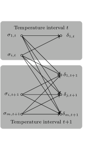
(a) Transportation Model

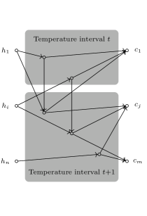
(b) Transshipment Model

Figure 1: In the transportation model (Cerda and Westerberg 1983), each hot stream $i$ supplies $\sigma_{i,t}$ units of heat in temperature interval $t$ which can be received, in the same or a lower temperature interval, by a cold stream $j$ which demands $\delta_{j,t}$ units of heat in $t$. In the transshipment model (Papoulias and Grossmann 1983), there are also intermediate nodes transferring residual heat to a lower temperature interval. This figure is adapted from Furman and Sahinidis (2004).

Transshipment Model (Papoulias and Grossmann 1983)

As illustrated in Figure 1(b), the transshipment formulation transfers heat from hot streams to cold streams via intermediate transshipment nodes. In each temperature interval, the heat entering a transshipment node either transfers to a cold stream in the same temperature interval or it descends to the transshipment node of the subsequent temperature interval as residual heat.

Binary variable $y_{i,j}$ is 1 if hot stream $i\in H$ is matched with cold stream $j\in C$ and 0 otherwise. Variable $q_{i,j,t}$ represents the heat received by cold stream $j\in C$ in temperature interval $t\in T$ originally exported by hot stream $i\in H$. Variable $r_{i,s}$ represents the residual heat of hot stream $i\in H$ that descends from temperature interval $s$ to temperature interval $s+1$. Parameter $U_{i,j}$ is a big-M parameter bounding the heat exchanged between hot stream $i\in H$ and cold stream $j\in C$, e.g. $U_{i,j}=\min\{h_{i},c_{j}\}$. The problem is formulated:

min $$\sum_{i\in H}\sum_{j\in C}y_{i,j}$$ (7)

$$\sum_{j\in C}q_{i,j,s}+r_{i,s}=\sigma_{i,s}+r_{i,s-1} i\in H,s\in T$$ (8)

$$r_{i,k}=0 i\in H$$ (9)

$$\sum_{i\in H}q_{i,j,t}=\delta_{j,t} j\in C,t\in T$$ (10)

$$\sum_{t\in T}q_{i,j,t}\leq U_{i,j}\cdot y_{i,j} i\in H,j\in C$$ (11)

$$y_{i,j}\in\{0,1\},\;q_{i,j,t},r_{i,s}\geq 0 i\in H,j\in C,s,t\in T$$ (12)

Expression (7) minimizes the number of matches. Equations (8)-(10) enforce heat conservation. Equation (11) allows positive heat exchange between hot stream $i\in H$ and cold stream $j\in C$ only if $(i,j)$ are matched.

3 Heuristics with Performance Guarantees

3.1 Computational Complexity

We briefly introduce $\mathcal{NP}$-completeness and basic computational complexity classes (Arora and Barak 2009, Papadimitriou 1994). A polynomial algorithm produces a solution for a computational problem with a running time polynomial to the size of the problem instance. There exist problems which admit a polynomial-time algorithm and others which do not. There is also the class of $\mathcal{NP}$-complete problems for which we do not know whether they admit a polynomial algorithm or not. The question of whether $\mathcal{NP}$-complete problems admit a polynomial algorithm is known as the $\mathcal{P}=\mathcal{NP}$ question. In general, it is conjectured that $\mathcal{P}\neq\mathcal{NP}$, i.e. $\mathcal{NP}$-complete problems are not solvable in polynomial time. An optimization problem is $\mathcal{NP}$-hard if its decision version is $\mathcal{NP}$-complete. A computational problem is strongly $\mathcal{NP}$-hard if it remains $\mathcal{NP}$-hard when all parameters are bounded by a polynomial to the size of the instance.

The minimum number of matches problem is known to be strongly $\mathcal{NP}$-hard, even in the special case of a single temperature interval. Furman and Sahinidis (2004) propose an $\mathcal{NP}$-hardness reduction from the well-known 3-Partition problem, i.e. they show that the minimum number of matches problem has difficulty equivalent to the 3-Partition problem. A presents an alternative $\mathcal{NP}$-hardness reduction from the bin packing problem. This alternative setting of the minimum number of matches problem gives new insight into the packing nature of the problem. A major contribution of this paper is to design efficient, greedy heuristics motivated by packing.

Theorem 1

There exists an $\mathcal{NP}$-hardness reduction from bin packing to the minimum number of matches problem with a single temperature interval.

Proof: See A.  

3.2 Approximation Algorithms

A heuristic with a performance guarantee is usually called an approximation algorithm (Vazirani 2001, Williamson and Shmoys 2011). Unless $\mathcal{P}=\mathcal{NP}$, there is no polynomial algorithm solving an $\mathcal{NP}$-hard problem. An approximation algorithm is a polynomial algorithm producing a near-optimal solution to an optimization problem. Formally, consider an an optimization problem, without loss of generality minimization, and a polynomial Algorithm $A$ for solving it (not necessarily to global optimality). For each problem instance $I$, let $C_{A}(I)$ and $C_{OPT}(I)$ be the algorithm’s objective value and the optimal objective value, respectively. Algorithm $A$ is $\rho$-approximate if, for every problem instance $I$, it holds that:

$$C_{A}(I)\leq\rho\cdot C_{OPT}(I).$$

That is, a $\rho$-approximation algorithm computes, in polynomial time, a solution with an objective value at most $\rho$ times the optimal objective value. The value $\rho$ is the approximation ratio of Algorithm $A$. To prove a $\rho$-approximation ratio, we proceed as depicted in Figure 2. For each problem instance, we compute analytically a lower bound $C_{LB}(I)$ of the optimal objective value, i.e. $C_{LB}(I)\leq C_{OPT}(I)$, and we show that the algorithm’s objective value is at most $\rho$ times the lower bound, i.e. $C_{A}(I)\leq\rho\cdot C_{LB}(I)$. The ratio of a $\rho$-approximation algorithm is tight if the algorithm is not $\rho-\epsilon$ approximate for any $\epsilon>0$. An algorithm is $O(f(n))$-approximate and $\Omega(f(n))$-approximate, where $f(n)$ is a function of an input parameter $n$, if the algorithm does not have an approximation ratio asymptotically higher and lower, respectively, than $f(n)$.

Figure 2: Analysis of an Approximation Algorithm

Approximation algorithms have been developed for two problem classes relevant to process systems engineering: heat exchanger networks (Furman and Sahinidis 2004) and pooling (Dey and Gupte 2015). Table 2 lists performance guarantees for the minimum number of matches problem; most are new to this manuscript.

Heuristic Abbrev. Section Performance Guarantee Running Time Single Temperature Interval Problem Simple Greedy SG 4.2 2^† (tight) $O(nm)$ Improved Greedy IG 4.2 1.5 (tight) $O(nm)$ Relaxation Rounding Heuristics Fractional LP Rounding FLPR 6.1 $O(k)^{\dagger}$, $O(U_{\max})$, $\Omega(n)$ 1 LP Lagrangian Relaxation Rounding LRR 6.2 2 LPs Covering Relaxation Rounding CRR 6.3 $O(nm)$ ILPs Water Filling Heuristics Water Filling MILP WFM 7 & 4.1 $O(k)^{\dagger}$, $\Omega(k)$ $O(k)$ MILPs Water Filling Greedy WFG 7 & 4.2 $O(k)^{\dagger}$, $\Omega(k)$ $O(nmk)$ Greedy Packing Heuristics Largest Heat Match LP-based LHM-LP 8.2 $O(\log n+\log(h_{\max}/\epsilon))$ $O(n^{2}m^{2})$ LPs Largest Heat Match Greedy LHM 8.2 $O(n^{2}m^{2}k)$ Largest Fraction Match LFM 8.3 $O(n^{2}m^{2}k)$ Shortest Stream SS 8.4 $O(nmk)$

Table 2: Performance guarantees for the minimum number of matches problem. The performance guarantees marked ${\dagger}$ are from Furman and Sahinidis (2004); all others are new to this manuscript.

4 Single Temperature Interval Problem

This section proposes efficient algorithms for the single temperature interval problem. Using graph theoretic properties, we obtain: (i) a novel, efficiently solvable MILP formulation without big-M constraints and (ii) an improved 3/2-approximation algorithm. Of course, the single temperature interval problem is not immediately applicable to the minimum number of matches problem with multiple temperature intervals. But designing efficient approximation algorithms for the single temperature interval is the first, essential step before considering multiple temperature intervals. Additionally, the water filling heuristics introduced in Section 7 repeatedly solve the single temperature interval problem.

In the single temperature interval problem, a feasible solution can be represented as a bipartite graph $G=(H\cup C,M)$ in which there is a node for each hot stream $i\in H$, a node for each cold stream $j\in C$ and the set $M\subseteq H\times C$ specifies the matches. B shows the existence of an optimal solution whose graph $G$ does not contain any cycle. A connected graph without cycles is a tree, so $G$ is a forest consisting of trees. B also shows that the number $v$ of edges in $G$, i.e. the number of matches, is related to the number $\ell$ of trees with the equality $v=n+m-\ell$. Since $n$ and $m$ are input parameters, minimizing the number of matches in a single temperature interval is equivalent to finding a solution whose graph consists of a maximal number $\ell$ of trees.

4.1 Novel MILP Formulation

We propose a novel MILP formulation for the single temperature interval problem. In an optimal solution without cycles, there can be at most $\min\{n,m\}$ trees. From a packing perspective, we assume that there are $\min\{n,m\}$ available bins and each stream is placed into exactly one bin. If a bin is non-empty, then its content corresponds to a tree of the graph. The objective is to find a feasible solution with a maximum number of bins.

To formulate the problem as an MILP, we define the set $B=\{1,2,\ldots,\min\{n,m\}\}$ of available bins. Binary variable $x_{b}$ is 0 if bin $b\in B$ is empty and 1, otherwise. A binary variable $w_{i,b}$ indicates whether hot stream $i\in H$ is placed into bin $b\in B$. Similarly, a binary variable $z_{j,b}$ specifies whether cold stream $j\in C$ is placed into bin $b\in B$. Then, the minimum number of matches problem can be formulated:

max $$\sum_{b\in B}x_{b}$$ (13)

$$x_{b}\leq\sum_{i\in H}w_{i,b} b\in B$$ (14)

$$x_{b}\leq\sum_{j\in C}z_{j,b} b\in B$$ (15)

$$\sum_{b\in B}w_{i,b}=1 i\in H$$ (16)

$$\sum_{b\in B}z_{j,b}=1 j\in C$$ (17)

$$\sum_{i\in H}w_{i,b}\cdot h_{i}=\sum_{j\in C}z_{j,b}\cdot c_{j} b\in B$$ (18)

$$x_{b},w_{i,b},z_{j,b}\in\{0,1\} b\in B,i\in H,j\in C$$ (19)

Expression (13), the objective function, maximizes the number of bins. Equations (14) and (15) ensure that a bin is used if there is at least one stream in it. Equations (16) and (17) enforce that each stream is assigned to exactly one bin. Finally, Eqs. (18) ensure the heat conservation of each bin. Note that, unlike the transportation and transshipment models, Eqs. (13)-(18) do not use a big-M parameter. D formulates the single temperature interval problem without heat conservation. Eqs. (25)-(30) are similar to Eqs. (13)-(19) except (i) they drop constraints (14) and (ii) equalities (16) & (18) become inequalities (27) & (29).

4.2 Improved Approximation Algorithm

Furman and Sahinidis (2004) propose a greedy 2-approximation algorithm for the minimum number of matches problem in a single temperature interval. We show that their analysis is tight. We also propose an improved, tight $1.5$-approximation algorithm by prioritizing matches with equal heat loads and exploiting graph theoretic properties.

The simple greedy (SG) algorithm considers the hot and the cold streams in non-increasing heat load order (Furman and Sahinidis 2004). Initially, the first hot stream is matched to the first cold stream and an amount $\min\{h_{1},c_{1}\}$ of heat is transferred between them. Without loss of generality $h_{1}>c_{1}$, which implies that an amount $h_{1}-c_{1}$ of heat load remains to be transferred from $h_{1}$ to the remaining cold streams. Subsequently, the algorithm matches $h_{1}$ to $c_{2}$, by transferring $\min\{h_{1}-c_{1},c_{2}\}$ heat. The same procedure repeats with the other streams until all remaining heat load is transferred.

Algorithm 1 Simple Greedy (SG), developed by Furman and Sahinidis (2004), is applicable to one temperature interval only.

1:Sort the streams so that $h_{1}\geq h_{2}\geq\ldots\geq h_{n}$ and $c_{1}\geq c_{2}\geq\ldots\geq c_{m}$.

2:Set $i=1$ and $j=1$.

3:while there is remaining heat load to be transferred do

4:     Transfer $q_{i,j}=\min\{h_{i},c_{j}\}$

5:     Set $h_{i}=h_{i}-q_{i,j}$ and $c_{j}=c_{j}-q_{i,j}$

6:     if $h_{i}=0$, then set $i=i+1$

7:     if $c_{j}=0$, then set $j=j+1$

8:end while

Furman and Sahinidis (2004) show that Algorithm SG is 2-approximate for one temperature interval. Our new result in Theorem 2 shows that this ratio is tight.

Theorem 2

Algorithm SG achieves an approximation ratio of 2 for the single temperature interval problem and it is tight.

Proof: See B.  

Algorithm IG improves Algorithm SG by: (i) matching the pairs of hot and cold streams with equal heat loads and (ii) using the acyclic property in the graph representation of an optimal solution. In practice, hot and cold process streams are unlikely to have equal supplies and demands of heat, so discussing equal heat loads is largely a thought experiment. But the updated analysis allows us to claim an improved performance bound on Algorithm SG. Additionally, the notion of matching roughly equivalent supplies and demands inspires the Section 8.3 Largest Fraction Match First heuristic.

Algorithm 2 Improved Greedy (IG) is applicable to one temperature interval only.

1:for each pair of hot stream $i$ and cold stream $j$ s.t. $h_{i}=c_{j}$ do

2:     Transfer $h_{i}$ amount of heat load (also equal to $c_{j}$) between them and remove them.

3:end for

4:Run Algorithm SG with respect to the remaining streams.

Theorem 3

Algorithm IG achieves an approximation ratio of 1.5 for the single temperature interval problem and it is tight.

Proof: See B.  

5 Maximum Heat Computations with Match Restrictions

This section discusses computing the maximum heat that can be feasibly exchanged in a minimum number of matches instance. Section 5.1 discusses the specific instance of two streams and thereby reduces the value of big-M parameter $U_{i,j}$. Sections 5.2 & 5.3 generalize Section 5.1 from 2 streams to any number of the candidate matches. Section 5.2 is limited to a restricted subset of matches in a single temperature interval. Section 5.3 calculates the maximum heat that can be feasibly exchanged for the most general case of multiple temperature intervals. These maximum heat computations are an essential ingredient of our heuristic methods and aim in using a match in the most profitable way. They also answer the feasibility of the minimum number of matches problem.

5.1 Two Streams and Big-M Parameter Computation

A common way of computing the big-M parameters is setting $U_{i,j}=\min\{h_{i},c_{j}\}$ for each $i\in H$ and $j\in C$. Gundersen et al. (1997) propose a better method for calculating the big-M parameter. Our novel Greedy Algorithm MHG (Maximum Heat Greedy) obtains tighter $U_{i,j}$ bounds than either the trivial bounds or the Gundersen et al. (1997) bounds by exploiting the transshipment model structure.

Given hot stream $i$ and cold stream $j$, Algorithm MHG computes the maximum amount of heat that can be feasibly exchanged between $i$ and $j$ in any feasible solution. Algorithm MHG is tight in the sense that there is always a feasible solution where streams $i$ and $j$ exchange exactly $U_{i,j}$ units of heat. Note that, in addition to $U_{i,j}$, the algorithm computes a value $q_{i,s,j,t}$ of the heat exchanged between each hot stream $i\in H$ in temperature interval $s\in T$ and each cold stream $j\in C$ in temperature interval $t\in T$, so that $\sum_{s,t\in T}q_{i,s,j,t}=U_{i,j}$. These $q_{i,s,j,t}$ values are required by greedy packing heuristics in Section 8.

Algorithm 3 is a pseudocode of Algorithm MHG. The correctness, i.e. the maximality of the heat exchanged between $i$ and $j$, is a corollary of the well known maximum flow - minimum cut theorem. Initially, the procedure transfers the maximum amount of heat across the same temperature interval; $q_{i,u,s,u}=\min\{\sigma_{i,u},\delta_{j,u}\}$ for each $u\in T$. The remaining heat is transferred greedily in a top down manner, with respect to the temperature intervals, by accounting heat residual capacities. For each temperature interval $u\in T$, the heat residual capacity $R_{u}=\sum_{i=1}^{n}\sum_{s=1}^{u}\sigma_{i,s}-\sum_{j=1}^{m}\sum_{t=1}^{u}\delta_{j,t}$ imposes an upper bound on the amount of heat that may descend from temperature intervals $1,2,\ldots,u$ to temperature intervals $u+1,u+2,\ldots,k$.

Algorithm 3 Maximum Heat Greedy (MHG)

Input: Hot stream $i\in H$ and cold stream $j\in C$

1:$\vec{q}\leftarrow\vec{0}$

2:for $u=1,2,\ldots,k-1$ do

3:     $R_{u}=\sum_{i=1}^{n}\sum_{s=1}^{u}\sigma_{i,s}-\sum_{j=1}^{m}\sum_{t=1}^{u}\delta_{j,t}$

4:end for

5:for $u=1,2,\ldots,k$ do

6:     $q_{i,u,j,u}\leftarrow\min\{\sigma_{i,u},\delta_{j,u}\}$

7:     $\sigma_{i,u}\leftarrow\sigma_{i,u}-q_{i,u,j,u}$

8:     $\delta_{j,u}\leftarrow\delta_{j,u}-q_{i,u,j,u}$

9:end for

10:for $s=1,2,\ldots,k-1$ do

11:     for $t=s+1,s+2,\ldots,k$ do

12:         $q_{i,s,j,t}=\min\{\sigma_{i,s},\delta_{j,t},\min_{s\leq u\leq t-1}\{R_{u}\}\}$

13:         $\sigma_{i,s}\leftarrow\sigma_{i,s}-q_{i,s,j,t}$

14:         $\delta_{j,t}\leftarrow\delta_{j,t}-q_{i,s,j,t}$

15:         for $u=s,s+1,s+2,\ldots,t-1$ do

16:              $R_{u}\leftarrow R_{u}-q_{i,s,j,t}$

17:         end for

18:     end for

19:end for

20:Return $\vec{q}$

5.2 Single Temperature Interval

Given an instance of the single temperature interval problem and a subset $M$ of matches, the maximum amount of heat that can be feasibly exchanged between the streams using only the matches in $M$ can be computed by solving MaxHeatLP. Like the single temperature interval algorithms of Section 4, MaxHeatLP is not directly applicable to a minimum number of matches problem with multiple temperature intervals. But MaxHeatLP is an important part of our water filling heuristics. For simplicity, MaxHeatLP drops temperature interval indices for variables $q_{i,j}$.

$$\begin{aligned} \text{max}&\sum_{(i,j)\in M}q_{i,j}\\ &\sum_{j\in C}q_{i,j}\leq h_{i}&i\in H\\ &\sum_{i\in H}q_{i,j}\leq c_{j}&j\in C\\ &q_{i,j}\geq 0&i\in H,j\in C\end{aligned}$$ (MaxHeatLP)

5.3 Multiple Temperature Intervals

Maximizing the heat exchanged through a subset of matches across multiple temperature intervals can solved with an LP that generalizes MaxHeatLP. The generalized LP must satisfy the additional requirement that, after removing a maximum heat exchange, the remaining instance is feasible. Feasibility is achieved using residual capacity constraints which are essential for the efficiency of greedy packing heuristics (see Section 8.1).

Given a set $M$ of matches, let $A(M)$ be the set of quadruples $(i,s,j,t)$ such that a positive amount of heat can be feasibly transferred via the transportation arc with endpoints the nodes $(i,s)$ and $(j,t)$. The set $A(M)$ does not contain any quadruple $(i,s,j,t)$ with: (i) $s>t$, (ii) $\sigma_{i,s}=0$, (iii) $\delta_{j,t}=0$, or (iv) $(i,j)\not\in M$. Let $V^{H}(M)$ and $V^{C}(M)$ be the set of transportation vertices $(i,s)$ and $(j,t)$, respectively, that appear in $A(M)$. Similarly, given two fixed vertices $(i,s)\in V^{H}(M)$ and $(j,t)\in V^{C}(M)$, we define the sets $V_{i,s}^{C}(M)$ and $V_{j,t}^{H}(M)$ of their respective neighbors in $A(M)$.

Consider a temperature interval $u\in T$. We define by $A_{u}(M)\subseteq A(M)$ the subset of quadruples with $s\leq u<t$, for $u\in T$. The total heat transferred via the arcs in $A_{u}(M)$ must be upper bounded by $R_{u}=\sum_{i=1}^{n}\sum_{s=1}^{u}\sigma_{i,s}-\sum_{j=1}^{m}\sum_{t=1}^{u}\delta_{j,t}$. Furthermore, $A(M)$ eliminates any quadruple $(i,s,j,t)$ with $R_{u}=0$, for some $s\leq u<t$. Finally, we denote by $T(M)$ the subset of temperature intervals affected by the matches in $M$, i.e. if $u\in T(M)$, then there exists a quadruple $(i,s,j,t)\in A(M)$, with $s\leq u<t$. The procedure $MHLP(M)$ is based on solving the following LP:

$$\max \sum_{(i,s,j,t)\in A(M)}q_{i,s,j,t}$$ (20)

$$\sum_{(j,t)\in V_{i,s}^{C}(M)}q_{i,s,j,t}\leq\sigma_{i,s} (i,s)\in V^{H}(M)$$ (21)

$$\sum_{(i,s)\in V_{j,t}^{H}(M)}q_{i,s,j,t}\leq\delta_{j,t} (j,t)\in V^{C}(M)$$ (22)

$$\sum_{(i,s,j,t)\in A_{u}(M)}q_{i,s,j,t}\leq R_{u} u\in T(M)$$ (23)

$$q_{i,s,j,t}\geq 0 (i,s,j,t)\in A(M)$$ (24)

Expression (20) maximizes the total exchanged heat by using only the matches in $M$. Constraints (21) and (22) ensure that each stream uses only part of its available heat. Constraints (23) enforce the heat residual capacities.

6 Relaxation Rounding Heuristics

This section investigates relaxation rounding heuristics for the minimum number of matches problem. These heuristics begin by optimizing an efficiently-solvable relaxation of the original MILP. The efficiently-solvable relaxation allows violation of certain constraints, so that the optimal solution(s) is (are) typically infeasible in the original MILP. The resulting infeasible solutions are subsequently rounded to feasible solutions for the original MILP. We consider 3 types of relaxations. Section 6.1 relaxes the integrality constraints and proposes fractional LP rounding. Section 6.2 relaxes the big-M constraints, i.e. Eqs. (4), and uses Lagrangian relaxation rounding. Section 6.3 relaxes the heat conservation equations, i.e. Eqs. (2)-(3), and takes an approach based on covering relaxations. Figure 3 shows the main components of relaxation rounding heuristics.

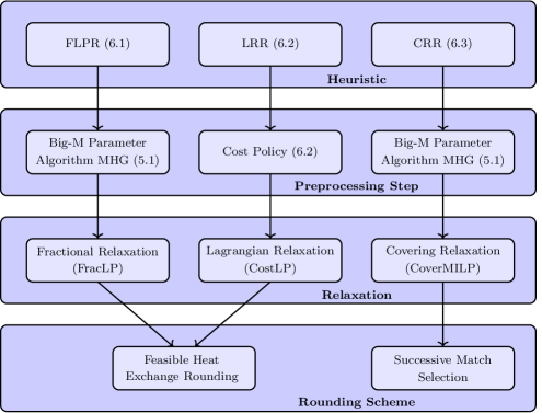
Figure 3: The main components of relaxation rounding heuristics are (i) a preprocessing step, (ii) a relaxation, and (iii) a rounding scheme. The preprocessing step constructs the relaxation. Fractional relaxation and covering relaxation require big-M parameter computations, while Lagrangian relaxation minimum cost LP requires cost calculations. FLPR and LRR compute a feasible heat exchange between all streams, i.e. values to variables $q_{i,s,j,t}$, by solving their respective relaxations and round the relaxed solutions according to Algorithm 4. Heuristic CRR adds matches incrementally until it ends up with a feasible solution. Feasibility is determined using the maximum heat LP in Section 5.3.

6.1 Fractional LP Rounding

The LP rounding heuristic, originally proposed by Furman and Sahinidis (2004), transforms an optimal fractional solution for the transportation MILP to a feasible integral solution. We show that the fractional LP can be solved efficiently via network flow techniques. We observe that, in the worst case, the heuristic produces a weak solution if it starts with an arbitrary optimal solution of the fractional LP. We derive a novel performance guarantee showing that the heuristic is efficient when the heat of each chosen match $(i,j)$ is close to big-M parameter $U_{i,j}$, in the optimal fractional solution.

Consider the fractional LP obtained by replacing the integrality constraints $y_{i,j}\in\{0,1\}$ of the transportation MILP, i.e. Eqs. (1)-(6), with the constraints $0\leq y_{i,j}\leq 1$, for each $i\in H$ and $j\in C$:

$$\begin{aligned} \min&\sum_{i\in H}\sum_{j\in C}y_{i,j}&\\ &\sum_{j\in C}\sum_{t\in T}q_{i,s,j,t}=\sigma_{i,s}&i\in H,s\in T\\ &\sum_{i\in H}\sum_{s\in T}q_{i,s,j,t}=\delta_{j,t}&j\in C,t\in T\\ &\sum_{s,t\in T}q_{i,s,j,t}\leq U_{i,j}\cdot y_{i,j}&i\in H,j\in C\\ &q_{i,s,j,t}=0&\;\;i\in H,j\in C,s,t\in T:s\leq t\\ &0\leq y_{i,j}\leq 1,\;q_{i,s,j,t}\geq 0&i\in H,j\in C,\;s,t\in T\end{aligned}$$ (FracLP)

FracLP can be solved via minimum cost flow methods. Figure 4 illustrates a network $N$, i.e. a minimum cost flow problem instance, such that finding a minimum cost flow in $N$ is equivalent to optimizing the fractional LP. Network $N$ is a layered graph with six layers of nodes: (i) a source node $S$, (ii) a node for each hot stream $i\in H$, (iii) a node for each pair $(i,s)$ of hot stream $i\in H$ and temperature interval $s\in T$, (iv) a node for each pair $(j,t)$ for each cold stream $j\in C$ and temperature interval $t\in T$, (v) a node for each cold stream $j\in C$, and (vi) a destination node $D$. We add: (i) the arc $(S,i)$ with capacity $h_{i}$ for each $i\in H$, (ii) the arc $(i,(i,s))$ with capacity $\sigma_{i,s}$ for each $i\in H$ and $s\in T$, (iii) the arc $((i,s),(j,t))$ with infinite capacity for each $i\in H$, $j\in C$ and $s,t\in T$, (iv) the arc $((j,t),j)$ with capacity $\delta_{j,t}$ for each $j\in H$ and $t\in T$, and (v) the arc $(j,D)$ with capacity $c_{j}$ for each $j\in C$. Each arc $((i,s),(j,t))$ has cost $1/U_{i,j}$ for $i\in H$, $j\in C$ and $s,t\in T$. Every other arc has zero cost. Any flow of cost $\sum_{i}h_{i}$ on network $N$ is equivalent to a feasible solution for FracLP with the same cost and vice versa.

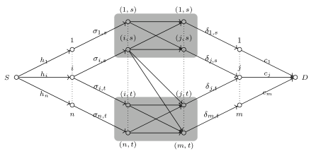
Figure 4: Minimum cost network flow formulation of FracLP. The heat is modeled as flow transferred from a source node $S$ to a destination node $D$. All finite capacities are labelled above the corresponding arcs. The cost is incurred in each arc between node $(i,s)\in H\times T$ and node $(j,t)\in C\times T$ under the condition that heat flows to the same or a lower temperature interval.

Furman and Sahinidis (2004) observe that any feasible solution of FracLP can be rounded to a feasible solution of the original problem via Algorithm 4, a simple greedy procedure that we call FLPR. Given a problem instance $I$, the procedure $FractionalLP(I)$ computes an optimal solution of FracLP. We denote by $(\vec{y}^{f},\vec{q}^{f})$ the optimal fractional solution.

Algorithm 4 Fractional LP Rounding (FLPR) (Furman and Sahinidis 2004)

1:$(\vec{y}^{f},\vec{q}^{f})\leftarrow FractionalLP(I)$ $\triangleright$ (FracLP) solving, Section 6.1

2:$\vec{q}\leftarrow\vec{q}^{f}$

3:for each $i\in H$ and $j\in C$ do

4:     if $\sum_{s,t\in T}q_{i,s,j,t}>0$ then

5:         $y_{i,j}\leftarrow 1$

6:     else

7:         $y_{i,j}\leftarrow 0$

8:     end if

9:end for

10:Return $(\vec{y},\vec{q})$

An inherent drawback of the Furman and Sahinidis (2004) approach is the existence of optimal fractional solutions with unnecessary matches. Theorem 4 shows that Algorithm FLPR performance is bad in the worst case, even for instances with a single temperature interval. The proof, given in C, can be extended so that unnecessary matches occur across multiple temperature intervals.

Theorem 4

Algorithm FLPR is $\Omega(n)$-approximate.

Proof: See C.  

Consider an optimal fractional solution to FracLP and suppose that $M\subseteq H\times C$ is the set of pairs of streams exchanging a positive amount of heat. For each $(i,j)\in M$, denote by $L_{i,j}$ the heat exchanged between hot stream $i$ and cold stream $j$. We define:

$$\phi(M)=\min_{(i,j)\in M}\left\{\frac{L_{i,j}}{U_{i,j}}\right\}$$

as the filling ratio, which corresponds to the minimum portion of an upper bound $U_{i,j}$ filled with the heat $L_{i,j}$, for some match $(i,j)$. Given an optimal fractional solution with filling ratio $\phi(M)$, Theorem 5 obtains a $1/\phi(M)$-approximation ratio for FLPR.

Theorem 5

Given an optimal fractional solution with a set $M$ of matches and filling ratio $\phi(M)$, FLPR produces a $\left(1/\phi(M)\right)$-approximate integral solution.

Proof: See C.  

In the case where all heat supplies and demands are integers, the integrality of the minimum cost flow polytope and Theorem 5 imply that FLPR is $U_{\max}$-approximate, where $U_{\max}=\max_{(i,j)\in H\times C}\{U_{i,j}\}$ is the biggest big-M parameter. A corollary of the $L_{i,j}/U_{i,j}$ ratio is that a fractional solution transferring heat $L_{i,j}$ close to capacity $U_{i,j}$ corresponds to a good integral solution. For example, if the optimal fractional solution satisfies $L_{i,j}>0.5\cdot U_{i,j}$, for every used match $(i,j)$ such that $L_{i,j}\neq 0$, then FLPR gives a 2-approximate integral solution. Finally, branch-and-cut repeatedly solves the fractional problem, so our new bound proves the big-M parameter’s relevance for exact methods. Because performance guarantee of FLPR scales with the big-M parameters $U_{i,j}$, we improve the heuristic performance by computing a small big-M parameter $U_{i,j}$ using Algorithm MHG in Section 5.1.

6.2 Lagrangian Relaxation Rounding

Furman and Sahinidis (2004) design efficient heuristics for the minimum number of matches problem by applying the method of Lagrangian relaxation and relaxing the big-M constraints. This approach generalizes Algorithm FLPR by approximating the fractional cost of every possible match $(i,j)\in H\times C$ and solving an appropriate LP using these costs. We present the LP and revisit different ways of approximating the fractional match costs.

In a feasible solution, the fractional cost $\lambda_{i,j}$ of a match $(i,j)$ is the cost incurred per unit of heat transferred via $(i,j)$. In particular,

$$\lambda_{i,j}=\left\{\begin{array}[]{ll}1/L_{i,j},&\mbox{if $L_{i,j}>0$, and}\\ 0,&\mbox{if $L_{i,j}=0$}\end{array}\right.$$

where $L_{i,j}$ is the heat exchanged via $(i,j)$. Then, the number of matches can be expressed as $\sum_{i,s,j,t}\lambda_{i,j}\cdot q_{i,s,j,t}$. Furman and Sahinidis (2004) propose a collection of heuristics computing a single cost value for each match $(i,j)$ and constructing a minimum cost solution. This solution is rounded to a feasible integral solution equivalently to FLPR.

Given a cost vector $\vec{\lambda}$ of the matches, a minimum cost solution is obtained by solving:

$$\begin{aligned} \text{min}&\sum_{i\in H}\sum_{j\in C}\sum_{s,t\in T}\lambda_{i,j}\cdot q_{i,s,j,t}\\ &\sum_{j\in C}\sum_{t\in T}q_{i,s,j,t}=\sigma_{i,s}&i\in H,s\in T\\ &\sum_{i\in H}\sum_{s\in T}q_{i,s,j,t}=\delta_{j,t}&j\in C,t\in T\\ &q_{i,s,j,t}\geq 0&i\in H,j\in C,\;s,t\in T\end{aligned}$$ (CostLP)

A challenge in Lagrangian relaxation rounding is computing a cost $\lambda_{i,j}$ for each hot stream $i\in H$ and cold stream $j\in C$. We revisit and generalize policies for selecting costs.

Cost Policy 1 (Maximum Heat)

Matches that exchange large amounts of heat incur low fractional cost. This observation motivates selecting $\lambda_{i,j}=1/U_{i,j}$, for each $(i,j)\in H\times C$, where $U_{i,j}$ is an upper bound on the heat that can be feasibly exchanged between $i$ and $j$. In this case, Lagrangian relaxation rounding is equivalent to FLPR (Algorithm 4).

Cost Policy 2 (Bounds on the Number of Matches)

This cost selection policy uses lower bounds $\alpha_{i}$ and $\beta_{j}$ on the number of matches of hot stream $i\in H$ and cold stream $j\in C$, respectively, in an optimal solution. Given such lower bounds, at least $\alpha_{i}$ cost is incurred for the $h_{i}$ heat units of $i$ and at least $\beta_{j}$ cost is incurred for the $c_{j}$ units of $j$. On average, each heat unit of $i$ is exchanged with cost at least ${\alpha_{i}}/{h_{i}}$ and each heat unit of $j$ is exchanged with cost at least ${\beta_{j}}/{c_{j}}$. So, the fractional cost of each match $(i,j)\in H\times C$ can be approximated by setting $\lambda_{i,j}={\alpha_{i}}/{h_{i}}$, $\lambda_{i,j}={\beta_{j}}/{c_{j}}$ or $\lambda_{i,j}=\frac{1}{2}(\frac{\alpha_{i}}{h_{i}}+\frac{\beta_{j}}{c_{j}})$.

Furman and Sahinidis (2004) use lower bounds $\alpha_{i}=1$ and $\beta_{j}=1$, for each $i\in H$ and $j\in C$. We show that, for any choice of lower bounds $\alpha_{i}$ and $\beta_{j}$, this cost policy for selecting $\lambda_{i,j}$ is not effective. Even when $\alpha_{i}$ and $\beta_{j}$ are tighter than 1, all feasible solutions of CostLP attain the same cost. Consider any feasible solution $(\vec{y},\vec{q})$ and the fractional cost $\lambda_{i,j}=\alpha_{i}/h_{i}$ for each $(i,j)\in H\times C$. Then the cost of $(\vec{y},\vec{q})$ in CostLP is:

$$\sum_{i\in H}\sum_{j\in C}\sum_{s,t\in T}\lambda_{i,j}\cdot q_{i,s,j,t}=\sum_{i\in H}\sum_{j\in C}\sum_{s,t\in T}\frac{\alpha_{i}}{h_{i}}\cdot q_{i,s,j,t}=\sum_{i\in H}\alpha_{i}.$$

Since every feasible solution in (CostLP) has cost $\sum_{i\in H}\alpha_{i}$, Lagrangian relaxation rounding returns an arbitrary solution. Similarly, if $\lambda_{i,j}={\beta_{j}}/{c_{j}}$ for $(i,j)\in H\times C$, every feasible solution has cost $\sum_{j\in C}\beta_{j}$. If $\lambda_{i,j}=\frac{1}{2}(\frac{\alpha_{i}}{h_{i}}+\frac{\beta_{j}}{c_{j}})$, all feasible solutions have the same cost $1/2\cdot(\sum_{i\in H}\alpha_{i}+\sum_{j\in C}\beta_{j})$.

Cost Policy 3 (Existing Solution)

This method of computing costs uses an existing solution. The main idea is to use the actual fractional costs for the solution’s matches and a non-zero cost for every unmatched streams pair. A minimum cost solution with respect to these costs may improve the initial solution. Suppose that $M$ is the set of matches in the initial solution and let $L_{i,j}$ be the heat exchanged via $(i,j)\in M$. Furthermore, let $U_{i,j}$ be an upper bound on the heat exchanged between $i$ and $j$ in any feasible solution. Then, a possible selection of costs is $\lambda_{i,j}=1/L_{i,j}$ if $(i,j)\in M$, and $\lambda_{i,j}=1/U_{i,j}$ otherwise.

6.3 Covering Relaxation Rounding

This section proposes a novel covering relaxation rounding heuristic for the minimum number of matches problem. The efficiency of Algorithm FLPR depends on lower bounding the unitary cost of the heat transferred via each match. The goal of the covering relaxation is to use these costs and lower bound the number of matches in a stream-to-stream to basis by relaxing heat conservation. The heuristic constructs a feasible integral solution by solving successively instances of the covering relaxation.

Consider a feasible MILP solution and suppose that $M$ is the set of matches. For each hot stream $i\in H$ and cold stream $j\in C$, denote by $C_{i}(M)$ and $H_{j}(M)$ the subsets of cold and hot streams matched with $i$ and $j$, respectively, in $M$. Moreover, let $U_{i,j}$ be an upper bound on the heat that can be feasibly exchanged between $i\in H$ and $j\in C$. Since the solution is feasible, it must be true that $\sum_{j\in C_{i}(M)}U_{i,j}\geq h_{i}$ and $\sum_{i\in H_{j}(M)}U_{i,j}\geq c_{j}$. These inequalities are necessary, though not sufficient, feasibility conditions. By minimizing the number of matches while ensuring these conditions, we obtain a covering relaxation:

$$\begin{aligned} \text{min}&\sum_{i\in H}\sum_{j\in C}y_{i,j}\\ &\sum_{j\in C}y_{i,j}\cdot U_{i,j}\geq h_{i}&i\in H\\ &\sum_{i\in H}y_{i,j}\cdot U_{i,j}\geq c_{j}&j\in C\\ &y_{i,j}\in\{0,1\}&i\in H,j\in C\end{aligned}$$ (CoverMILP)

In certain cases, the matches of an optimal solution to CoverMILP overlap well with the matches in a near-optimal solution for the original problem. Our new Covering Relaxation Rounding (CRR) heuristic for the minimum number of matches problem successively solves instances of the covering relaxation CoverMILP. The heuristic chooses new matches iteratively until it terminates with a feasible set $M$ of matches. In the first iteration, Algorithm CRR constructs a feasible solution for the covering relaxation and adds the chosen matches in $M$. Then, Algorithm CRR computes the maximum heat that can be feasibly exchanged using the matches in $M$ and stores the computed heat exchanges in $\vec{q}$. In the second iteration, the heuristic performs same steps with respect to the smaller updated instance $(\vec{\sigma}^{\prime},\vec{\delta}^{\prime})$, where $\sigma_{i,s}^{\prime}=\sigma_{i,s}-\sum_{j,t}q_{i,s,j,t}$ and $\delta_{j,t}^{\prime}=\delta_{j,t}-\sum_{i,s}q_{i,s,j,t}$. The heuristic terminates when all heat is exchanged.

Algorithm 5 is a pseudocode of heuristic CRR. Procedure $CoveringRelaxation(\vec{\sigma},\vec{\delta})$ produces an optimal subset of matches for the instance of the covering relaxation in which the heat supplies and demands are specified by the vectors $\vec{\sigma}$ and $\vec{\delta}$, respectively. Procedure $MHLP(\vec{\sigma},\vec{\delta},M)$ (LP-based Maximum Heat) computes the maximum amount of heat that can be feasibly exchanged by using only the matches in $M$ and is based on solving the LP in Section 5.3.

Algorithm 5 Covering Relaxation Rounding (CRR)

1:$M\leftarrow\emptyset$

2:$\vec{q}\leftarrow\vec{0}$

3:$r\leftarrow\sum_{i\in H}h_{i}$

4:while $r>0$ do

5:     For each $i\in H$ and $s\in T$, set $\sigma_{i,s}^{\prime}\leftarrow\sigma_{i,s}-\sum_{j\in C}\sum_{t\in T}q_{i,s,j,t}$

6:     For each $j\in C$ and $t\in T$, set $\delta_{j,t}^{\prime}\leftarrow\delta_{j,t}-\sum_{i\in H}\sum_{s\in T}q_{i,s,j,t}$

7:     $M^{\prime}\leftarrow CoveringRelaxation(\vec{\sigma}^{\prime},\vec{\delta}^{\prime})$ $\triangleright$ (CoverMILP) solving, Section 6.3

8:     $M\leftarrow M\cup M^{\prime}$

9:     $\vec{q}\leftarrow MHLP(\vec{\sigma},\vec{\delta},M^{\prime})$ $\triangleright$ Equations (20) - (24) LP solving, Section 5.3

10:     $r\leftarrow\sum_{i\in H}h_{i}-\sum_{i\in H}\sum_{j\in C}\sum_{s,t\in T}q_{i,s,j,t}$

11:end while

7 Water Filling Heuristics

This section introduces water filling heuristics for the minimum number of matches problem. These heuristics produce a solution iteratively by exchanging the heat in each temperature interval, in a top down manner. The water filling heuristics use, in each iteration, an efficient algorithm for the single temperature interval problem (see Section 4).

Figure 5 shows the main idea of a water filling heuristic for the minimum number of matches problem with multiple temperature intervals. The problem is solved iteratively in a top-down manner, from the highest to the lowest temperature interval. Each iteration produces a solution for one temperature interval. The main components of a water filling heuristic are: (i) a maximum heat procedure which reuses matches from previous iterations and (ii) an efficient single temperature interval algorithm.

(a) Top Down Temperature Interval Structure

(b) Excess Heat Descending

Figure 5: A water filling heuristic computes a solution by exploiting the top down temperature interval structure and moving from the higher to the lower temperature interval. In each temperature interval $t$, the heuristic isolates the streams with positive heat at $t$, it matches them and descends the excess heat to the next interval which is sequentially solved.

Given a set $M$ of matches and an instance $(\vec{\sigma_{t}},\vec{\delta}_{t})$ of the problem in the single temperature interval $t$, the procedure $MHS(\vec{\sigma}_{t},\vec{\delta}_{t},M)$ (Maximum Heat for Single temperature interval) computes the maximum heat that can be exchanged between the streams in $t$ using only the matches in $M$. At a given temperature interval $t$, the $MHS$ procedure solves the LP in Section 5.2. The procedure $SingleTemperatureInterval(\vec{\sigma}_{t},\vec{\delta}_{t})$ produces an efficient solution for the single temperature interval problem with a minimum number of matches and total heat to satisfy one cold stream. $SingleTemperatureInterval(\vec{\sigma}_{t},\vec{\delta}_{t})$ either: (i) solves the MILP exactly (Water Filling MILP-based or WFM) or (ii) applies the improved greedy approximation Algorithm IG in Section 4 (Water Filling Greedy or WFG). Both water filling heuristics solve instances of the single temperature interval problem in which there is no heat conservation, i.e. the heat supplied by the hot streams is greater or equal than the heat demanded by the cold streams. The exact WFM uses the MILP proposed in Eqs. (25) - (30) of D. The greedy heuristic WFG adapts Algorithm IG by terminating when the entire heat demanded by the cold streams has been transferred. After addressing the single temperature interval, the excess heat descends to the next temperature interval. Algorithm 6 represents our water filling approach in pseudocode. Figure 6 shows the main components of water filling heuristics.

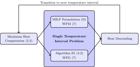
Figure 6: Water filling heuristics solve the temperature intervals serially in a top-down manner and keep composition feasible. The main components are (i) a maximum heat computation re-using higher temperature interval matches, (ii) a single temperature interval problem algorithm, and (iii) excess heat descending between consecutive temperature intervals. Heuristic WFM uses the D MILP formulation for solving the single temperature interval problem, while heuristic WFG uses the Section 4.2 Algorithm IG.

Algorithm 6 Water Filling (WF)

1:$M\leftarrow\emptyset$

2:$\vec{q}\leftarrow\vec{0}$

3:for $t=1,2,\ldots,k$ do

4:     if $t\neq 1$ then

5:         $\vec{q}\;^{\prime}\leftarrow MHS(\vec{\sigma}_{t},\vec{\delta}_{t},M)$ $\triangleright$ (MaxHeatLP) solve, Section 5.2

6:         $\vec{q}\leftarrow\vec{q}+\vec{q}\;^{\prime}$

7:         For each $i\in H$, set $\sigma_{i,t}\leftarrow\sigma_{i,t}-\sum_{j\in C}\sum_{t\in T}q_{i,j,t}^{\prime}$

8:         For each $j\in C$, set $\delta_{j,t}\leftarrow\delta_{j,t}-\sum_{i\in H}\sum_{s\in T}q_{i,j,t}^{\prime}$

9:     end if

10:     $(M^{\prime},\vec{q}\;^{\prime})\leftarrow SingleTemperatureInterval(\vec{\sigma}_{t},\vec{\delta}_{t})$ $\triangleright$ Eqs (25 - 30) or Alg IG, Sec 4.2

11:     $M\leftarrow M\cup M^{\prime}$

12:     $\vec{q}\leftarrow\vec{q}+\vec{q}\;^{\prime}$

13:     if $t\neq k$ then

14:         for $i\in H$ do

15:              $\vec{\sigma}_{i,t+1}\leftarrow\vec{\sigma}_{i,t+1}+(\vec{\sigma}_{i,t}-\sum_{j}q_{i,j,t})$ (excess heat descending)

16:         end for

17:     end if

18:end for

Theorem 6

Algorithms WFG and WFM are $\Omega(k)$-approximate.

Proof: See D.  

8 Greedy Packing Heuristics

This section proposes greedy heuristics motivated by the packing nature of the minimum number of matches problem. Each greedy packing heuristic starts from an infeasible solution with zero heat transferred between the streams and iterates towards feasibility by greedily selecting matches. The two main ingredients of such a heuristic are: (i) a match selection policy and (ii) a heat exchange policy for transferring heat via the matches. Section 8.1 observes that a greedy heuristic has a poor worst-case performance if heat residual capacities are not considered. Sections 8.2 - 8.4 define formally the greedy heuristics: (i) Largest Heat Match First, (ii) Largest Fraction Match First, and (iii) Smallest Stream First. Figure 7 shows the main components of greedy packing heuristics.

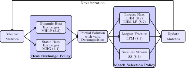
Figure 7: Greedy packing heuristics select matches iteratively one by one. The main components of greedy packing heuristics are (i) a heat exchange policy, and (ii) a match selection policy. Greedy packing heuristics apply these policies with respect to all unmatched stream pairs, in each iteration. Options for the heat exchange policy include dynamic heat exchange, which solves the Section 5.3 maximum heat LP, and static heat exchange, which uses the Section 5.1 greedy algorithm. Once the heat exchange policy has been applied for every unmatched pair of streams, a match selection policy chooses the new match, e.g. (i) with the largest heat (LHM), (ii) with the largest fraction (LFM), or (iii) of the shortest stream (SS).

8.1 A Pathological Example and Heat Residual Capacities

A greedy match selection heuristic is efficient if it performs a small number of iterations and chooses matches exchanging large heat load in each iteration. Our greedy heuristics perform large moves towards feasibility by choosing good matches in terms of: (i) heat and (ii) stream fraction. An efficient greedy heuristic should also be monotonic in the sense that every chosen match achieves a strictly positive increase on the covered instance size.

The Figure 8 example shows a pathological behavior of greedy non-monotonic heuristics. The instance consists of 3 hot streams, 3 cold streams and 3 temperature intervals. Hot stream $i\in H$ has heat supply $\sigma_{i,s}=1$ for $s=i$ and no supply in any other temperature interval. Cold stream $j\in C$ has heat demand $\delta_{j,t}=1$ for $t=j$ and no demand in any other temperature interval. Consider the heuristic which selects a match that may exchange the maximum amount of heat in each iteration. The matches $(h_{1},c_{2})$ and $(h_{2},c_{3})$ consist the initial selections. In the subsequent iteration, no match increases the heat that can be feasibly exchanged between the streams and the heuristic chooses unnecessary matches.

Figure 8: A bad example of a non monotonic heuristic. If a heuristic begins by matching $h_{1}$ with $c_{2}$ and $h_{2}$ with $c_{3}$, then many unnecessary matches might be required to end up with a feasible solution.

A sufficient condition enforcing strictly monotonic behavior and avoiding the above pathology, is for each algorithm iteration to satisfy the heat residual capacities. As depicted in Figure 9, a greedy heuristic maintains a set $M$ of selected matches together with a decomposition of the original instance $I$ into two instances $I^{A}$ and $I^{B}$. If $I=(H,C,T,\vec{\sigma},\vec{\delta})$, then it holds that $I^{A}=(H,C,T,\vec{\sigma}^{A},\vec{\delta}^{A})$ and $I^{B}=(H,C,T,\vec{\sigma}^{B},\vec{\delta}^{B})$, where $\mathbf{\sigma}=\vec{\sigma}^{A}+\vec{\sigma}^{B}$ and $\vec{\delta}=\vec{\delta}^{A}+\vec{\delta}^{B}$. The set $M$ corresponds to a feasible solution for $I^{A}$ and the instance $I^{B}$ remains to be solved. In particular, $I^{A}$ is obtained by computing a maximal amount of heat exchanged by using the matches in $M$ and $I^{B}$ is the remaining part of $I$. Initially, $I^{A}$ is empty and $I^{B}$ is exactly the original instance $I$. A selection of a match increases the total heat exchanged in $I^{A}$ and reduces it in $I^{B}$. E observes that a greedy heuristic is monotonic if $I^{B}$ is feasible in each iteration. Furthermore, $I^{B}$ is feasible if and only if $I^{A}$ satisfies the heat residual capacities $R_{u}=\sum_{i\in H}\sum_{s=1}^{u}\sigma_{i,s}-\sum_{j\in C}\sum_{t=1}^{u}\delta_{j,t}$, for $u\in T$.

Figure 9: Decomposition of a greedy packing heuristic. The problem instance $I$ is the union of the instance $I_{A}$ already solved by the heuristic and the instance $I_{B}$ that remains to be solved.

8.2 Largest Heat Match First

Our Largest Heat Match First heuristics arise from the idea that the matches should individually carry large amounts of heat in a near optimal solution. Suppose that $Q_{v}$ is the maximum heat that may be transferred between the streams using only a number $v$ of matches. Then, minimizing the number of matches is expressed as $\min\{v:Q_{v}\geq\sum_{i=1}^{n}h_{i}\}$. This observation motivates the greedy packing heuristic which selects matches iteratively until it ends up with a feasible set $M$ of matches exchanging $\sum_{i=1}^{n}h_{i}$ units of heat. In each iteration, the heuristic chooses a match maximizing the additional heat exchanged. Our two variants of largest heat matches heuristics are: (i) LP-based Largest Heat Match (LHM-LP) and (ii) Greedy Largest Heat Match (LHM).

Heuristic LHM-LP uses the $MHLP(M)$ (LP-based Maximum Heat) procedure to compute the maximum heat that can be transferred between the streams using only the matches in the set $M$. This procedure is repeated $O(nm)$ times in each iteration, once for every candidate match, and solves an LP incorporating the proposed heat residual capacities. Algorithm 7 is an LHM-LP heuristic using the LP in Section 5.3. The algorithm maintains a set $M$ of chosen matches and selects a new match $(i^{\prime},j^{\prime})$ to maximize $MHLP(M\cup(i^{\prime},j^{\prime}))$.

Algorithm 7 Largest Heat Match First LP-based (LHM-LP)

1:$M\leftarrow\emptyset$

2:$r\leftarrow\sum_{i\in H}h_{i}$

3:while $r>0$ do

4:     $(i^{\prime},j^{\prime})\leftarrow\arg\max_{(i,j)\in H\times C\setminus M}\{MHLP(M\cup\{(i,j)\})\}$ $\triangleright$ Eqs (20 - 24), Sec 5.3

5:     $M\leftarrow M\cup\{(i^{\prime},j^{\prime})\}$

6:     $r\leftarrow\sum_{i\in H}h_{i}-MHLP(M)$

7:end while

8:Return $M$

Theorem 7

Algorithm LHM-LP is $O(\log n+\log\frac{h_{\max}}{\epsilon})$-approximate, where $\epsilon$ is the required precision.

Proof: See E.  

LHM-LP heuristic is polynomial-time in the worst case. The $i$-th iteration solves $nm-i+1$ LP instances which sums to solving a total of $\sum_{i=1}^{nm}(nm-i+1)=O(n^{2}m^{2})$ LP instances in the worst case. However, for large instances, the algorithm is time consuming because of this iterative LP solving. So, we also propose an alternative, time-efficient greedy approach. The new heuristic version builds a solution by selecting matches and deciding the heat exchanges, without modifying them in subsequent iterations.

The new approach for implementing the heuristic, that we call LHM, requires the $MHG(\vec{\sigma},\vec{\delta},i,j)$ procedure. Given an instance $(\vec{\sigma},\vec{\delta})$ of the problem, it computes the maximum heat that can be feasibly exchanged between hot stream $i\in H$ and cold stream $j\in C$, as defined in Section 5.1. The procedure also computes a corresponding value $q_{i,s,j,t}$ of heat exchanged between $i\in H$ in temperature interval $s\in T$ and $j\in C$ in temperature interval $t\in T$. LHM maintains a set $M$ of currently chosen matches together with their respective vector $\vec{q}$ of heat exchanges. In each iteration, it selects the match $(i^{\prime},j^{\prime})$ and heat exchanges $q^{\prime}$ between $i^{\prime}$ and $j^{\prime}$ so that the value $MHG(\vec{\sigma},\vec{\delta},i^{\prime},j^{\prime})$ is maximum. Algorithm 8 is a pseudocode of this heuristic.

Algorithm 8 Largest Heat Match First Greedy (LHM)

1:$M\leftarrow\emptyset$

2:$\vec{q}\leftarrow\vec{0}$

3:$r\leftarrow\sum_{i\in H}h_{i}$

4:while $r>0$ do

5:     $(i^{\prime},j^{\prime},\vec{q}\;^{\prime})\leftarrow\arg\max_{(i,j)\in H\times C\setminus M}\{MHG(\vec{\sigma},\vec{\delta},i,j)\}$ $\triangleright$ Algorithm MHG, Section 5.1

6:     $M\leftarrow M\cup\{(i^{\prime},j^{\prime})\}$

7:     $\vec{q}\leftarrow\vec{q}+\vec{q}\;^{\prime}$

8:     For each $s\in T$, set $\sigma_{i^{\prime},s}\leftarrow\sigma_{i^{\prime},s}-\sum_{t\in T}q_{i^{\prime},s,j^{\prime},t}^{\prime}$

9:     For each $t\in T$, set $\delta_{j^{\prime},t}\leftarrow\delta_{j^{\prime},t}-\sum_{s\in T}q_{i^{\prime},s,j^{\prime},t}^{\prime}$

10:     $r\leftarrow r-\sum_{s,t\in T}q_{i^{\prime},s,j^{\prime},t}^{\prime}$

11:end while

12:Return $M$

8.3 Largest Fraction Match First

The heuristic Largest Fraction Match First (LFM) exploits the bipartite nature of the problem by employing matches which exchange large fractions of the stream heats. Consider a feasible solution with a set $M$ of matches. Every match $(i,j)\in M$ covers a fraction $\sum_{s,t\in T}\frac{q_{i,s,j,t}}{h_{i}}$ of hot stream $i\in H$ and a fraction $\sum_{s,t\in T}\frac{q_{i,s,j,t}}{c_{j}}$ of cold stream $j\in C$. The total covered fraction of all streams is equal to $\sum_{(i,j)\in M}\sum_{s,t\in T}\left(\frac{q_{i,s,j,t}}{h_{i}}+\frac{q_{i,s,j,t}}{c_{j}}\right)=n+m$. Suppose that $F_{v}$ is the maximum amount of total stream fraction that can be covered using no more than $v$ matches. Then, minimizing the number of matches is expressed as $\min\{v:F_{v}\geq n+m\}$. Based on this observation, the main idea of LFM heuristic is to construct iteratively a feasible set of matches, by selecting the match covering the largest fraction of streams, in each iteration. That is, LFM prioritizes proportional matches in a way that high heat hot streams are matched with high heat cold streams and low heat hot streams with low heat cold streams. In this sense, it generalizes the idea of Algorithm IG for the single temperature interval problem (see Section 4), according to which it is beneficial to match streams of (roughly) equal heat.

An alternative that would be similar to LHM-LP is an LFM heuristic with an $MFLP(M)$ (LP-based Maximum Fraction) procedure computing the maximum fraction of streams that can be covered using only a given set $M$ of matches. Like the LHM-LP heuristic, this procedure would be based on solving an LP (see E), except that the objective function maximizes the total stream fraction. The LFM heuristic can be also modified to attain more efficient running times using Algorithm $MHG$, as defined in Section 5.1. In each iteration, the heuristic selects the match $(i,j)$ with the highest value $\frac{U_{i,j}^{\prime}}{h_{i}}+\frac{U_{i,j}^{\prime}}{c_{j}}$, where $U_{i,j}^{\prime}$ is the maximum heat that can be feasibly exchanged between $i$ and $j$ in the remaining instance.

8.4 Smallest Stream Heuristic

Subsequently, we propose Smallest Stream First (SS) heuristic based on greedy match selection, which also incorporates stream priorities so that a stream is involved in a small number of matches. Let $\alpha_{i}$ and $\beta_{j}$ be the number of matches of hot stream $i\in H$ and cold stream $j\in C$, respectively. Minimizing the number of matches problem is expressed as $\min\{\sum_{i\in H}\alpha_{i}\}$, or equivalently $\min\{\sum_{j\in C}\beta_{j}\}$. Based on this observation, we investigate heuristics that specify a certain order of the hot streams and match them one by one, using individually a small number of matches. Such a heuristic requires: (i) a stream ordering strategy and (ii) a match selection strategy. To reduce the number of matches of small hot streams, heuristic SS uses the order $h_{1}\leq h_{2}\leq\ldots\leq h_{n}$.

In each iteration, the next stream is matched with a low number of cold streams using a greedy match selection strategy; we use greedy LHM heuristic. Observe that SS heuristic is more efficient in terms of running time compared to the other greedy packing heuristics, because it solves a subproblem with only one hot stream in each iteration. Algorithm 9 is a pseudocode of SS heuristic. Note that other variants of ordered stream heuristics may be obtained in a similar way. The heuristic uses the $MHG$ algorithm in Section 5.1.

Algorithm 9 Smallest Steam First (SS)

1:Sort the hot streams in non-decreasing order of their heat loads, i.e. $h_{1}\leq h_{2}\leq\ldots\leq h_{n}$.

2:$M\leftarrow\emptyset$

3:$\vec{q}\leftarrow\vec{0}$

4:for $i\in H$ do

5:     $r\leftarrow h_{i}$

6:     while $r>0$ do

7:         $(i,j^{\prime},\vec{q}\;^{\prime})\leftarrow\arg\max_{j\in C}\{MHG(\vec{\sigma},\vec{\delta},i,j)\}$ $\triangleright$ Algorithm MHG, Section 5.1

8:         $M\leftarrow M\cup\{(i,j^{\prime})\}$

9:         $\vec{q}\leftarrow\vec{q}+\vec{q}\;^{\prime}$

10:         For each $s\in T$, set $\sigma_{i,s}\leftarrow\sigma_{i,s}-\sum_{t\in T}q_{i,s,j^{\prime},t}^{\prime}$

11:         For each $t\in T$, set $\delta_{j^{\prime},t}\leftarrow\delta_{j^{\prime},t}-\sum_{s\in T}q_{i,s,j^{\prime},t}^{\prime}$

12:         $r\leftarrow r-\sum_{s,t\in T}q_{i^{\prime},s,j^{\prime},t}^{\prime}$

13:     end while

14:end for

15:Return $M$

9 Numerical Results

This section evaluates the proposed heuristics on three test sets. Section 9.1 provides information on system specifications and benchmark instances. Section 9.2 presents computational results of exact methods and shows that commercial, state-of-the-art approaches have difficult solving moderately-sized instances to global optimality. Section 9.3 evaluates experimentally the heuristic methods and compares the obtained results with those reported by Furman and Sahinidis (2004). All result tables are provided in G. Letsios et al. (2017) provide test cases and source code for the paper’s computational experiments.

9.1 System Specification and Benchmark Instances

All computations are run on an Intel Core i7-4790 CPU 3.60GHz with 15.6 GB RAM running 64-bit Ubuntu 14.04. CPLEX 12.6.3 and Gurobi 6.5.2 solve the minimum number of matches problem exactly. The mathematical optimization models and heuristics are implemented in Python 2.7.6 and Pyomo 4.4.1 (Hart et al. 2011, 2012).

We use problem instances from two existing test sets (Furman and Sahinidis 2004, Chen et al. 2015b). We also generate two collections of larger test cases. The smaller of the two sets uses work of Grossmann (2017). The larger of the two sets was created using our own random generation method. An instance of general heat exchanger network design consists of streams and utilities with inlet, outlet temperatures, flow rate heat capacities and other parameters. F shows how a minimum number of matches instances arises from the original instance of general heat exchanger network design.

The Furman (2000) test set consists of test cases from the engineering literature. Table 4 reports bibliographic information on the origin of these test cases. We manually digitize this data set and make it publicly available for the first time (Letsios et al. 2017). Table 4 lists the 26 problem instance names and information on their sizes. The total number streams and temperature intervals varies from 6 to 38 and from 5 to 32, respectively. Table 4 also lists the number of binary and continuous variables as well as the number of constraints in the transshipment MILP formulation.

The Chen et al. (2015a, b) test set consists of 10 problem instances. These instances are classified into two categories depending on whether they consist of balanced or unbalanced streams. Test cases with balanced streams have flowrate heat capacities in the same order of magnitude, while test cases with unbalanced streams have dissimilar flowrate heat capacities spanning several orders of magnitude. The sizes of these instances range from 10 to 42 streams and from 12 to 35 temperature intervals. Table 4 reports more information on the size of each test case.

The Grossmann (2017) test set is generated randomly. The inlet, outlet temperatures of these instances are fixed while the values of flowrate heat capacities are generated randomly with fixed seeds. This test set contains 12 moderately challenging problems (see Table 4) with a classification into balanced and unbalanced instances, similarly to the Chen et al. (2015a, b) test set. The smallest problem involves 27 streams and 23 temperature intervals while the largest one consists of 43 streams and 37 temperature intervals.

The Large Scale test set is generated randomly. These instances have 80 hot streams, 80 cold streams, 1 hot utility and 1 cold utility. For each hot stream $i\in HS$, the inlet temperature $T_{\text{in},i}^{HS}$ is chosen uniformly at random in the interval $(30,400]$. Then, the outlet temperature $T_{\text{out},i}^{HS}$ is selected uniformly at random in the interval $[30,T_{\text{in},i}^{HS})$. Analogously, for each cold stream $j\in CS$, the outlet temperature $T_{\text{out},j}^{CS}$ is chosen uniformly at random in the interval $(20,400]$. Next, the inlet temperature $T_{\text{in},j}^{CS}$ is chosen uniformly at random in the interval $[20,T_{\text{out},j}^{CS})$. The flow rate heat capacities $FCp_{i}$ and $FCp_{j}$ of hot stream $i$ and cold stream $j$ are chosen as floating numbers with two decimal digits in the interval $[0,15]$. The hot utility has inlet temperature $T_{\text{in}}^{HU}=500$, outlet temperature $T_{\text{out}}^{HS}=499$, and cost $\kappa^{HU}=80$. The cold utility has inlet temperature $T_{\text{in}}^{CU}=20$, outlet temperature $T_{\text{out}}^{CU}=21$, and cost $\kappa^{CU}=20$. The minimum heat recovery approach temperature is $\Delta T_{\min}=10$.

9.2 Exact Methods

We evaluate exact methods using state-of-the-art commercial approaches. For each problem instance, CPLEX and Gurobi solve the Section 2 transportation and transshipment models. Based on the difficulty of each test set, we set a time limit for each solver run as follows: (i) 1800 seconds for the Furman (2000) test set, (ii) 7200 seconds for the Chen et al. (2015a, b) test set, and (iii) 14400 seconds for the Grossmann (2017) and large scale test sets. In each solver run, we set absolute gap 0.99, relative gap $4\%$, and maximum number of threads 1.

Table 5 reports the best found objective value, CPU time and relative gap, for each solver run. Observe that state-of-the-art approaches cannot, in general, solve moderately-sized problems with 30-40 streams to global optimality. For example, none of the test cases in the Grossmann (2017) or large scale test sets is solved to global optimality within the specified time limit. Table 9 contains the results reported by Furman and Sahinidis (2004) using CPLEX 7.0 with 7 hour time limit. CPLEX 7.0 fails to solve 4 instances to global optimality. Interestingly, CPLEX 12.6.3 still cannot solve 3 of these 4 instances with a 1.5 hour timeout.

Theoretically, the transshipment MILP is better than the transportation MILP because the former has asymptotically fewer variables. This observation is validated experimentally with the exception of very few instances, e.g. balanced10, in which the transportation model computes a better solution within the time limit. CPLEX and Gurobi are comparable and neither dominates the other. Instances with balanced streams are harder to solve, which highlights the difficulty introduced by symmetry, see Kouyialis and Misener (2017). The preceding numerical analysis refers to the extended transportation MILP. Table 6 compares solver performance to the reduced transportation MILP, i.e. a formulation removing redundant variables $q_{i,s,j,t}$ with $s>t$ and Equations (5). Note that modern versions of CPLEX and Gurobi show effectively no difference between the two formulations.

9.3 Heuristic Methods

We implement the proposed heuristics using Python and develop the LP models with Pyomo (Hart et al. 2011, 2012). We use CPLEX 12.6.3 with default settings to solve all LP models within the heuristic methods. Letsios et al. (2017) make the source code available. The following discussion covers the 48 problems with 43 streams or fewer. Section 9.4 discusses the 3 examples with 160 streams each.

The difficulty of solving the minimum number of matches problem to global optimality motivates the design of heuristic methods and approximation algorithms with proven performance guarantees. Tables 7 and 8 contain the computed objective value and CPU times, respectively, of the heuristics for all test cases. For the challenging Chen et al. (2015a, b) and Grossmann (2017) test sets, heuristic LHM-LP always produces the best solution. The LHM-LP running time is significantly higher compared to all heuristics due to the iterative LP solving, despite the fact that it is guaranteed to be polynomial in the worst case. Alternatively, heuristic SS produces the second best heuristic result with very efficient running times in the Chen et al. (2015a, b) and Grossmann (2017) test sets. Figure 10 depicts the performance ratio of the proposed heuristics using a box and whisker plot, where the computed objective value is normalized with the one found by CPLEX for the transshipment MILP. Figure 11 shows a box and whisker plot of the CPU times of all heuristics in $\log_{10}$ scale normalized by the minimum CPU time for each test case. Figure 12 shows a line chart verifying that our greedy packing approach produces better solutions than the relaxation rounding and water filling ones.

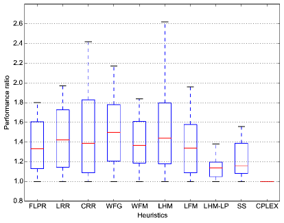
Figure 10: Box and whisker diagram of 48 heuristic performance ratios, i.e. computed solution / best known solution for the problems with 43 streams or fewer.

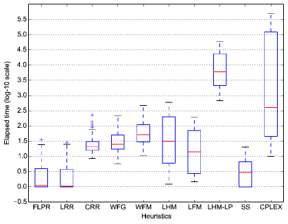
Figure 11: Box and whisker diagram of 48 CPU times ($\log_{10}$ scale) normalized by the minimum CPU time for each test case.

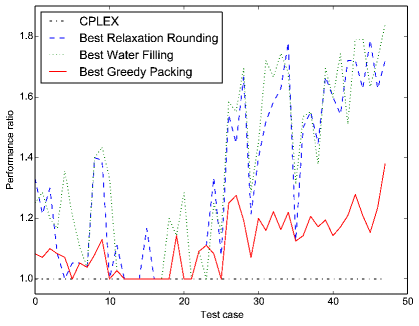
Figure 12: Line chart comparing the performance ratio, i.e. computed solution / best known solution, of the best computed result by heuristic methods: relaxation rounding, water filling, and greedy packing. This graph applies to the 48 problems with 43 streams or fewer.

Table 9 contains the heuristic results reported by Furman and Sahinidis (2004) and the ones obtained with our improved version of the FLPR, LRR, and WFG heuristics of Furman and Sahinidis (2004). Our versions of FLPR, LRR, and WFG perform better for the Furman and Sahinidis (2004) test set because of our new Algorithm MHG for tightening the big-M parameters. For example, out of the 26 instances, our version of FLPR performs strictly better than the Furman and Sahinidis (2004) version 20 times and worse only once (10sp1). To further explore the effect of the big-M parameter, Table 10 shows how different computations for the big-M parameter change the FLPR and LRR performance. Table 10 also demonstrates the importance of the big-M parameter on the transportation MILP fractional relaxation quality.

In particular, Table 10 compares the three big-M computation methods discussed in Section 5.1: (i) the trivial bounds, (ii) the Gundersen et al. (1997) method, and (iii) our greedy Algorithm MHG. Our greedy maximum heat algorithm dominates the other approaches for computing the big-M parameters. Algorithm MHG also outperforms the other two big-M computation methods by finding smaller feasible solutions via both Fractional LP Rounding and Lagrangian Relaxation Rounding. In the 48 test cases, Algorithm MHG produces the best FLPR and LRR feasible solutions in 46 and 43 test cases, respectively. Algorithm MHG is strictly best for 33 FLPR and 32 LRR test cases. Finally, Algorithm MHG achieves the tightest fractional MILP relaxation for all test instances.

Figure 10 and Table 7 show that our new CRR heuristic is competitive with the other relaxation rounding heuristics, performing as well or better than FLPR or LRR in 19 of the 48 test cases and strictly outperforming both FLPR and LRR in 8 test cases. Although CRR solves a sequence of MILPs, Figure 11 and Table 8 show that its running time is efficient compared to the other relaxation rounding heuristics.

Our water filling heuristics are equivalent to or better than Furman and Sahinidis (2004) for 25 of their 26 test set instances (all except 7sp2). In particular, our Algorithm WFG is strictly better than their WFG in 18 of 26 instances and is worse in just one. This improvement stems from the new 1.5-approximation algorithm for the single temperature interval problem (see Section 4.2). The novel Algorithm WFM is competitive with Algorithm WFG and produces equivalent or better feasible solutions for 37 of the 48 test cases. In particular, WFM has a better performance ratio than WFG (see Figure 10) and WFM is strictly better than WFG in all but 1 of the Grossmann (2017) instances. The strength of WFM highlights the importance of our new MILP formulation in Eqs. (13)-(19). At each iteration, WFM solves an MILP without big-M constraints and therefore has a running time in the same order of magnitude as its greedy counterpart WFG (see Figure 11).

In summary, our heuristics obtained via the relaxation rounding and water filling methods improve the corresponding ones proposed by Furman and Sahinidis (2004). Furthermore, greedy packing heuristics achieve even better results in more than $90\%$ of the test cases.

9.4 Larger Scale Instances

Although CPLEX and Gurobi do not converge to global optimality for many of the Furman (2000), Chen et al. (2015a, b), and Grossmann (2017) instances, the solvers produce the best heuristic solutions in all test cases. But the literature instances are only moderately sized. We expect that the heuristic performance improves relative to the exact approaches as the problem sizes increase. Towards a more complete numerical analysis, we randomly generate 3 larger scale instances with 160 streams each.

For larger problems, the running time may be important to a design engineer (Linnhoff and Hindmarsh 1983). We apply the least time consuming heuristic of each type for solving the larger scale instances, i.e. apply relaxation rounding heuristic FLPR, water filling heuristic WFG, and greedy packing heuristic SS. We also solve the transshipment model using CPLEX 12.6.3 with a 4h timeout. The results are in Table 11.

For these instances, greedy packing SS computes a better solution than the relaxation rounding FLPR heuristic or the water filling WFG heuristic, but SS has larger running time. In instance large-scale1, greedy packing SS computes 218, a better solution than the CPLEX value 219. Moreover, the CPLEX heuristic spent the first 1hr of computation time at solution 257 (18% worse than the solution SS obtains in 10 minutes) and the next 2hr of computation time at solution 235 (8% worse than the solution SS obtains in 10 minutes). Any design engineer wishing to interact with the results would be frustrated by these times.

In instance large-scale2, CPLEX computes a slightly better solution (239) than the SS heuristic (242). But the good CPLEX solution is computed slightly before the 4h timeout. For more than 3.5hr, the best CPLEX heuristic is 273 (13% worse than the solution SS obtains in 10 minutes). Finally, in instance large-scale0, CPLEX computes a significantly better solution (175) than the SS heuristic (233). But CPLEX computes the good solution after 2h and the incumbent is similar to the greedy packing SS solution for the first 2 hours. These findings demonstrate that greedy packing approaches are particularly useful when transitioning to larger scale instances.

Note that we could additionally study approaches to improve the heuristic performance of CPLEX, e.g. by changing CPLEX parameters or using a parallel version of CPLEX. But the point of this paper is to develop a deep understanding of a very important problem that consistently arises in process systems engineering (Floudas et al. 2012).

10 Discussion of Manuscript Contributions

This section reflects on this paper’s contributions and situates the work with respect to existing literature. We begin in Section 4 by designing efficient heuristics for the minimum number of matches problem with the special case of a single temperature interval. Initially, we show that the 2 performance guarantee by Furman and Sahinidis (2004) is tight. Using graph theoretic properties, we propose a new MILP formulation for the single temperature interval problem which does not contain any big-M constraints. We also develop an improved, tight, greedy 1.5-approximation algorithm which prioritizes stream matches with equal heat loads. Apart from the its independent interest, solving the single temperature interval problem is a major ingredient of water filling heuristics.

The multiple temperature interval problem requires big-M parameters. We reduce these parameters in Section 5 by computing the maximum amount of heat transfer with match restrictions. Initially, we present a greedy algorithm for exchanging the maximum amount of heat between two streams. This algorithm computes tighter big-M parameters than Gundersen et al. (1997). We also propose LP-based ways for computing the maximum exchanged heat using only a subset of the available matches. Maximum heat computations are fundamental ingredients of our heuristic methods and detect the overall problem feasibility. This paper emphasizes how tighter big-M parameters improve heuristics with performance guarantees, but notice that improving the big-M parameters will also tend to improve exact methods.

Section 6 further investigates the relaxation rounding heuristics of Furman and Sahinidis (2004). Furman and Sahinidis (2004) propose a heuristic for the minimum number of matches problem based on rounding the LP relaxation of the transportation MILP formulation (Fractional LP Rounding (FLPR)). Initially, we formulate the LP relaxation as a minimum cost flow problem showing that it can be solved with network flow techniques which are more efficient than generic linear programming. We derive a negative performance guarantee showing that FLPR has poor performance in the worst case. We also prove a new positive performance guarantee for FLPR indicating that its worst-case performance may be improved with tighter big-M parameters. Experimental evaluation shows that the performance of FLPR improves with our tighter algorithm for computing big-M parameters. Motivated by the method of Lagrangian Relaxation, Furman and Sahinidis (2004) proposed an approach generalizing FLPR by approximating the cost of the heat transferred via each match. We revisit possible policies for approximating the cost of each match. Interestingly, we show that this approach can be used as a generic method for potentially improving a solution of the minimum number of matches problem. Heuristic Lagrangian Relaxation Rounding (LRR) aims to improve the solution of FLPR in this way. Finally, we propose a new heuristic, namely Covering Relaxation Rounding (CRR), that successively solves instances of a new covering relaxation which also requires big-M parameters.

Section 7 defines water filling heuristics as a class of heuristics solving the minimum number of matches problem in a top-down manner, i.e. from highest to lowest temperature interval. Cerda et al. (1983) and Furman and Sahinidis (2004) have solution methods based on water filling. We improve these heuristics by developing novel, efficient ways for solving the single temperature interval problem. For example, heuristics MILP-based Water Filling (WFM) and Greedy Water Filling (WFG) incorporate the new MILP formulation (Eqs. 13-19) and greedy Algorithm IG, respectively. With appropriate LP, we further improve water filling heuristics by reusing in each iteration matches selected in previous iterations. Furman and Sahinidis (2004) showed a performance guarantee scaling with the number of temperature intervals. We show that this performance guarantee is asymptotically tight for water filling heuristics.

Section 8 develops a new greedy packing approach for designing efficient heuristics for the minimum the number of matches problem motivated by the packing nature of the problem. Greedy packing requires feasibility conditions which may be interpreted as a decomposition method analogous to pinch point decomposition, see Linnhoff and Hindmarsh (1983). Similarly to Cerda et al. (1983), stream ordering affects the efficiency of greedy packing heuristics. Based on the feasibility conditions, the LP in Eqs. (20)-(24) selects matches carrying a large amount of heat and incurring low unitary cost for exchanging heat. Heuristic LP-based Largest Heat Match (LHM-LM) selects matches greedily by solving instances of this LP. Using a standard packing argument, we obtain a new logarithmic performance guarantee. LHM-LP has a polynomial worst-case running time but is experimentally time-consuming due to the repeated LP solving. We propose three other greedy packing heuristic variants which improve the running time at the price of solution quality. These other variants are based on different time-efficient strategies for selecting good matches. Heuristic Largest Heat Match (LHM) selects matches exchanging high heat in a pairwise manner. Heuristic Largest Fraction Match (LFM) is inspired by the idea of our greedy approximation algorithm for the single temperature interval problem which prioritizes roughly equal matches. Heuristic Smallest Stream First (SS) is inspired by the idea of the tick-off heuristic (Linnhoff and Hindmarsh 1983) and produces matches in a stream to stream basis, where a hot stream is ticked-off by being matched with a small number of cold streams.

Finally, Section 9 shows numerically that our new way of computing the big-M parameters, our improved algorithms for the single temperature interval, and the other enhancements improve the performance of relaxation rounding and water-filling heuristics. The numerical results also show that our novel greedy packing heuristics typically find better feasible solutions than relaxation rounding and water-filling ones. But the tradeoff is that the relaxation rounding and water filling algorithms achieve very efficient run times.

11 Conclusion

In his PhD thesis, Professor Floudas showed that, given a solution to the minimum number of matches problem, he could solve a nonlinear optimization problem designing effective heat recovery networks. But the sequential HENS method cannot guarantee that promising minimum number of matches solutions will be optimal (or even feasible!) to Professor Floudas’ nonlinear optimization problem. Since the nonlinear optimization problem is relatively easy to solve, we propose generating many good candidate solutions to the minimum number of matches problem. This manuscript develops nine heuristics with performance guarantees to the minimum number of matches problem. Each of the nine heuristics is either novel or provably the best in its class. Beyond approximation algorithms, our work has interesting implications for solving the minimum number of matches problem exactly, e.g. the analysis into reducing big-M parameters or the possibility of quickly generating good primal feasible solutions.

Acknowledgments
We gratefully acknowledge support from EPSRC EP/P008739/1, an EPSRC DTP to G.K., and a Royal Academy of Engineering Research Fellowship to R.M.

Appendix A $\mathcal{NP}$-hardness Reduction

Theorem 1

There exists an $\mathcal{NP}$-hardness reduction from bin packing to the minimum number of matches problem with a single temperature interval.

Proof:
Initially, define the decision version of bin packing. A bin packing instance consists of a set $B=\{1,2,\ldots,m\}$ of bins, each bin of capacity $K$, and a set $O=\{1,2,\ldots,n\}$ of objects, where object $i\in O$ has size $s_{i}\in(0,K]$. The goal is to determine whether there exist a feasible packing $O_{1},O_{2},\ldots,O_{m}$ of the objects into the bins, where $O_{j}\subseteq O$ is the subset of objects packed in bin $j\in B$. Each object is placed in exactly one bin, i.e. $\cup_{j=1}^{m}O_{j}=O$ and $O_{j}\cap O_{j^{\prime}}=\emptyset$ for each $1\leq j<j^{\prime}\leq m$, and the total size of the objects in a bin do not exceed its capacity, i.e. $\sum_{i\in O_{j}}s_{i}\leq K$, for $j\in B$.

Consider an instance $(O,n,B,m)$ of bin packing. Construct an instance of the minimum number of matches problem with a single temperature interval by setting $H=O$, $h_{i}=s_{i}$ for $i=1,\ldots,n$, $C=B$ and $c_{j}=K$ for $j=1,\ldots,m$. We claim that bin packing has a feasible solution if and only if the constructed minimum number of matches instance is feasible using exactly $n$ matches.

To the first direction, consider a feasible packing $O_{1},\ldots,O_{m}$. For each $i\in H$ and $j\in C$, we obtain a solution for the minimum number of matches instance by setting $q_{i,j}=h_{i}$ if $i\in O_{j}$, and $q_{i,j}=0$, otherwise. By the constraints $\cup_{j=1}^{m}O_{j}=O$ and $O_{j}\cap O_{j^{\prime}}=\emptyset$ for each $1\leq j<j^{\prime}\leq m$, there is exactly one $j\in B$ such that $i\in O_{j}$. Hence, the number of matches is $|\{(i,j)\in H\times C:q_{i,j}>0\}|=n$ and $\sum_{j\in C}q_{i,j}=h_{i}$ for every $i\in H$. Since the capacity of bin $j\in B$ is not exceeded, we have that $\sum_{i\in O_{j}}s_{i}\leq K$, or equivalently $\sum_{i\in H}q_{i,j}\leq c_{j}$ for all $j\in C$. Thus, the obtained solution is feasible.

To the other direction, consider a feasible solution for the minimum number of matches instance. Obtain a feasible packing by placing object $i\in O$ in the bin $j$ if and only if $q_{i,j}>0$. Since the solution contains at most $n$ matches and $h_{i}>0$, for each $i\in H$, each hot stream $i\in H$ matches with exactly one cold stream $j\in C$ and it holds that $q_{i,j}=h_{i}$. That is, each object is placed in exactly one bin. Given that $\sum_{i\in H}q_{i,j}\leq c_{j}=K$, the bin capacity constraints are also satisfied.  

Appendix B Single Temperature Interval Problem

Lemma 8 concerns the structure of an optimal solution for the single temperature interval problem. It shows that the corresponding graph is acyclic and that the number of matches is related to the number of graph’s connected components (trees), if arc directions are ignored.

Lemma 8

Consider an instance $H$, $C$ of the single temperature interval problem. For each optimal solution $(\vec{y}^{*},\vec{q}^{*})$, there exists an integer $\ell^{*}\in[1,\min\{n,m\}]$ s.t.

• if arc directions are ignored, the corresponding graph $G(\vec{y}^{*},\vec{q}^{*})$ is a forest consisting of $\ell^{*}$ trees, i.e. there are no cycles, and

• $(\vec{y}^{*},\vec{q}^{*})$ contains $v^{*}=m+n-\ell^{*}$ matches.

Proof:
Assume that $G(\vec{y}^{*},\vec{q}^{*})$ contains a cycle, after removing arc directions. Moreover, let $M=\{(i_{1},j_{1}),(i_{2},j_{1}),(i_{2},j_{2}),(i_{3},j_{2}),\ldots,(i_{g},j_{g-1}),(i_{g},j_{g}),(i_{1},j_{g})\}$ be a subset of matches forming a cycle. Denote by $q_{\min}^{*}=\min\{q_{i,j}^{*}:(i,j)\in M\}$ the minimum amount of heat transferred via a match in $M$. Without loss of generality, assume that $q_{i_{1},j_{1}}^{*}=q_{\min}^{*}$. Starting from $(\vec{y}^{*},\vec{q}^{*})$, produce a feasible solution $(\vec{y},\vec{q})$ as follows. Set $q_{i_{1},j_{1}}=0$, $q_{i_{e},j_{e}}=q_{i_{e},j_{e}}^{*}-q_{\min}^{*}$ and $q_{i_{e},j_{e-1}}=q_{i_{e},j_{e-1}}^{*}+q_{\min}^{*}$, for $e=2,\ldots,g$, as well as $q_{i_{1},j_{g}}=q_{i_{1},j_{g}}^{*}+q_{\min}^{*}$. The new solution $(\vec{y},\vec{q})$ is feasible and has a strictly smaller number of matches compared to $(\vec{y}^{*},\vec{q}^{*})$, which is a contradiction.

Since $G(\vec{y}^{*},\vec{q}^{*})$ does not contain a cycle, it must be a forest consisting of $\ell^{*}$ trees (which we call bins from a packing perspective). Let $B=\{1,\ldots,\ell^{*}\}$ be the set of these trees and $M_{b}$ the subset of matches in tree $b\in B$. By definition, tree $b\in B$ contains $|M_{b}|$ matches (edges) and, therefore, $|M_{b}|+1$ streams (nodes). Furthermore, each stream appears in exactly one tree implying that $\sum_{b=1}^{\ell^{*}}|M_{b}|=n+m-\ell^{*}$. Thus, it holds that the number of matches in $(\vec{y}^{*},\vec{q}^{*})$ is equal to:

$$v=\sum_{b=1}^{\ell^{*}}|M_{b}|=n+m-\ell^{*}.\vspace{-24pt}$$

 

Theorem 2 that Algorithm SG, developed by Furman and Sahinidis (2004), is tight.

Theorem 2

Algorithm SG achieves an approximation ratio of 2 for the single temperature interval problem and it is tight.

Proof:
In the algorithm’s solution, the number $v$ of matches is equal to the number of steps that the algorithm performs. For each pair of streams $i\in H$ and $j\in C$ matched by the algorithm, at least one has zero remaining heat load exactly after they have been matched. Therefore, the number of steps is at most $v\leq n+m-1$. The optimal solution contains at least $v^{*}\geq\max\{n,m\}$. Hence, the algorithm is 2-approximate.

Consider a set of $n$ hot streams with heat loads $h_{i}=2n+1-i$ for $1\leq i\leq n$ and $m=n+1$ cold streams with $c_{j}=2n-j$, for $1\leq j\leq m$. As shown in Figure 13 for the special case $n=5$, the algorithm uses $2n$ matches while the optimal solution has $n+1$ matches. Hence, the 2 approximation ratio of Algorithm SG is asymptotically tight.  

(a) Algorithm SG: 10

(b) Optimal solution: 6

Figure 13: An instance showing the tightness of the 2 performance guarantee for Algorithm SG.

Lemma 9 formalizes the benefit of matching stream pairs with equal heat loads and indicates the way of manipulating these matches in the analysis of Algorithm IG and the proof of Theorem 3.

Lemma 9

Consider an instance $(H,C)$ of the single temperature interval problem and suppose that there exists a pair of streams $i\in H$ and $j\in C$ such that $h_{i}=c_{j}$. Then,

• there exists an optimal solution $(\vec{y}^{*},\vec{q}^{*})$ s.t. $q_{i,j}^{*}=h_{i}$, i.e. $i$ and $j$ are matched together,

• any $\rho$-approximate solution for $(H\setminus\{i\},C\setminus\{j\})$ is also $\rho$-approximate for $(H,C)$ with the addition of match $(i,j)$.

Proof:
Consider an optimal solution $(\vec{y}^{*},\vec{q}^{*})$ in which $i$ and $j$ are not matched solely to each other. Suppose that $i$ is matched with $j_{1},j_{2},\ldots,j_{m^{\prime}}$ while $j$ is matched with $i_{1},i_{2},\ldots,i_{n^{\prime}}$. Without loss of generality, $q_{i,j}^{*}=0$; the case $0<q_{i,j}^{*}<h_{i}$ is treated similarly. Starting from $(\vec{y}^{*},\vec{q}^{*})$, we obtain the slightly modified solution $(\vec{y},\vec{q})$ in which $i$ is matched only with $j$. The $c_{j}$ units of heat of $i_{1},i_{2},\ldots,i_{n^{\prime}}$ originally transferred to $j$ are now exchanged with $j_{1},j_{2},\ldots,j_{m^{\prime}}$, which are no longer matched with $i$. The remaining solution is not modified. Analogously to the proof of Theorem 2, we show that there can be at most $n^{\prime}+m^{\prime}-1$ new matches between the $n^{\prime}$ hot streams (i.e. $i_{1},i_{2},\ldots,i_{n^{\prime}}$) and the $m^{\prime}$ cold streams (i.e. $j_{1},j_{2},\ldots,j_{m^{\prime}}$) in $(\vec{y},\vec{q})$. By also taking into account the new match $(i,j)$, we conclude that there exists always a solution in which $i$ is only matched with $j$ and has no more matches than $(\vec{y}^{*},\vec{q}^{*})$.

Consider an optimal solution $(\vec{y}^{*},\vec{q}^{*})$ for $(H,C)$, in which there are $v^{*}$ matches and $i$ is matched only with $j$. An optimal solution for $(H\setminus\{i\},C\setminus\{j\})$ contains $v^{*}-1$ matches. Suppose that $(\vec{y},\vec{q})$ is the union of a $\rho$-approximate solution for $(H\setminus\{i\},C\setminus\{j\})$ and the match $(i,j)$. Let $v$ be the number of matches in $(\vec{y},\vec{q})$. Clearly, $v-1\leq\rho\cdot(v^{*}-1)$ which implies that $v\leq\rho\cdot v^{*}$, as $\rho\geq 1$.  

The following theorem shows a tight analysis for Algorithm IG.

Theorem 3

Algorithm IG achieves an approximation ratio of 1.5 for the single temperature interval problem and it is tight.

Proof:
By Theorem 2, Algorithm IG produces a solution $(\vec{y},\vec{q})$ with $v\leq n+m$ matches. Consider an optimal solution $(\vec{y}^{*},\vec{q}^{*})$. By Lemma 8, $(\vec{y}^{*},\vec{q}^{*})$ consists of $\ell^{*}$ trees and has $v^{*}=n+m-\ell^{*}$ matches. Due Lemma 9, we may assume that instance does not contain a pair of equal hot and cold streams. Hence, each tree in the optimal solution contains at least 3 streams, i.e. $\ell^{*}\leq(n+m)/3$. Thus, $v^{*}\geq(2/3)(n+m)$ and we conclude that $v\leq(3/2)v^{*}$.

For the tightness of our analysis, consider an instance of the problem with $n$ hot streams, where $h_{i}=4n-2i$ for $i=1,\ldots,n$, and $m=2n$ cold streams such that $c_{j}=4n-2j-1$ for $j=1,\ldots,n$ and $c_{j}=1$ for $j=n+1,\ldots,2n$. Algorithm IG uses $3n$ matches, while the optimal solution uses $2n$ matches. Hence the $3/2$ approximation ratio of the algorithm is tight. Figures 14(a) and 14(b) show the special case with $n=4$.  

(a) Algorithm IG: 11

(b) Optimal solution: 8

Figure 14: An instance showing the tightness of the 1.5 performance guarantee for Algorithm IG.

Appendix C Relaxation Rounding Heuristics

Theorem 4

Algorithm FLPR is $\Omega(n)$-approximate.

Proof:
We construct a minimum number of matches instance for which Algorithm FLPR produces a solution $\Omega(n)$ times far from the optimal solution. This instance consists of a single temperature interval and an equal number of hot and cold streams, i.e. $n=m$, with the same heat load $h_{i}=n$ and $c_{j}=n$, for each $i\in H$ and $j\in C$. Because of the single temperature interval, we ignore the temperature interval indices of the variables $\vec{q}$. In the optimal solution, each hot stream is matched with exactly one cold stream and there are $v^{*}=n$ matches in total. Given that there exist feasible solutions such that $q_{i,j}=n$, for every possible $i\in H$ and $j\in C$, the algorithm computes the upper bound $U_{i,j}=n$. In an optimal fractional solution, it holds that $q_{i,j}^{f}=1$, for each $i\in H$ and $j\in C$. In this case, Algorithm FLPR sets $y_{i,j}=1$ for each pair of streams $i\in H$, $j\in C$ and uses a total number of matches equal to $v=\sum_{i\in H}\sum_{j\in C}y_{i,j}=\Omega(n^{2})$. Therefore, it is $\Omega(n)$-approximate.  

Theorem 5

Given an optimal fractional solution with a set $M$ of matches and filling ratio $\phi(M)$, FLPR produces a $\frac{1}{\phi(M)}$-approximate integral solution.

Proof:
We denote Algorithm FLPR’s solution and the optimal fractional solution by $(\vec{y},\vec{q})$ and $(\vec{y}^{f},\vec{q}^{f})$, respectively. Moreover, suppose that $(\vec{y}^{*},\vec{q}^{*})$ is an optimal integral solution. Let $M\subseteq H\times C$ be the set of matched pairs of streams by the algorithm, i.e. $y_{i,j}=1$, if $(i,j)\in M$, and $y_{i,j}=0$, otherwise. Then, it holds that:

$$\sum_{(i,j)\in M}y_{i,j} =\sum_{(i,j)\in M}\frac{U_{i,j}}{L_{i,j}}\sum_{s,t\in T}\frac{q_{i,s,j,t}}{U_{i,j}}$$

$$\leq\frac{1}{\phi(M)}\sum_{(i,j)\in M}\sum_{s,t\in T}\frac{q_{i,s,j,t}^{f}}{U_{i,j}}$$

$$\leq\frac{1}{\phi(M)}\sum_{(i,j)\in M}y_{i,j}^{f}$$

$$\leq\frac{1}{\phi(M)}\sum_{i\in H}\sum_{j\in C}y_{i,j}^{*}.$$

The first equality is obtained by using the fact that, for each $(i,j)\in M$, it holds that $y_{i,j}=\frac{U_{i,j}}{L_{i,j}}\frac{L_{i,j}}{U_{i,j}}$ and $L_{i,j}=\sum_{s,t\in T}q_{i,s,j,t}$. The first inequality is true by the definition of the filling ratio $\phi(M)$ and the fact that $\vec{q}=\vec{q}^{f}$. The second inequality holds by the big-M constraint of the fractional relaxation. The final inequality is valid due to the fact that the optimal fractional solution is a lower bound on the optimal integral solution.  

Appendix D Water Filling Heuristics

The reformulated MILP in Eqs. (25)-(30) solves the single temperature interval problem without heat conservation. It is similar to the MILP in Eqs. (13)-(19) with heat conservation, except that it does not contain constraints (14) while Equalities (16) and (18) become the inequalities (27) and (29). In the single temperature interval problem with (without) heat conservation, the total heat of hot streams is equal to (greater than or equal to) the demand of the cold streams. Each water filling algorithm step solves the single temperature interval problem without heat conservation. All heat demands of cold streams are satisfied and the excess heat supply of hot streams descends to the subsequent temperature interval.

max $$\sum_{b\in B}x_{b}$$ (25)

$$x_{b}\geq\sum_{j\in C}z_{j,b} b\in B$$ (26)

$$\sum_{b\in B}w_{i,b}\leq 1 i\in H$$ (27)

$$\sum_{b\in B}z_{j,b}=1 j\in C$$ (28)

$$\sum_{i\in H}w_{i,b}\cdot h_{i}\geq\sum_{j\in C}z_{j,b}\cdot c_{j} b\in B$$ (29)

$$x_{b},w_{i,b},z_{j,b}\in\{0,1\} b\in B,i\in H,j\in C$$ (30)

Theorem 6 shows an asymptotically tight performance guarantee for water filling heuristics proportional to the number of temperature intervals. The positive performance guarantee implies the proof of Furman and Sahinidis (2004).

Theorem 6

Algorithms WFG and WFM are $\Theta(k)$-approximate (i.e. both $O(k)$-approximate and $\Omega(k)$-approximate).

Proof:
A water filling algorithm solves an instance of the single temperature interval problem in each temperature interval $t=1,\ldots,k$. This instance consists of at most $n$ hot streams and at most $m$ cold streams. By Theorem 2, algorithms WFG and WFM introduce at most $n+m$ new matches in each temperature interval and produce a solution with $v\leq k(n+m)$ matches. In the optimal solution, each hot and cold stream appears in at least one match which means that $v^{*}\geq\max\{n,m\}$ matches are chosen in total. So, $v\leq 2k\cdot v^{*}$.

On the negative side, we show a lower bound on the performance guarantee of algorithms WFG and WFM using the extension of the problem instance in Figure 15 with an equal number of hot streams, cold streams and temperature intervals, i.e. $m=n=k$. Each hot stream $i\in H$ has heat supply $\sigma_{i,s}\in\{0,1\}$ and each cold stream $j\in C$ has heat demand $\delta_{j,t}\in\{0,1\}$, for each $s,t\in T$. Hot stream $i$ has unit heat in temperature intervals $\{1,\ldots,k-i+1\}$ and no supply elsewhere. Cold stream $j$ demands unit heat in temperature intervals $\{j,\ldots,k\}$ and no demand elsewhere. In the optimal solution, hot stream $i$ is matched with cold stream $j=i$ and there are $v^{*}=k$ matches in total. Algorithms WFG and WFM produce the same solution in which hot stream $i$ is matched with cold streams $\{1,2,\ldots,k-i+1\}$, where $j=i$, and there are $v=O(k^{2})$ matches in total.  

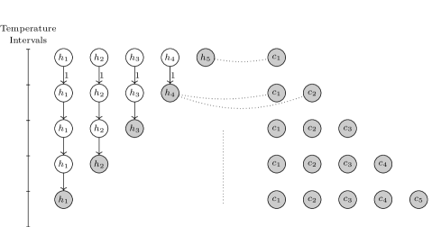
Figure 15: An instance showing (asymptotically) the tightness of the $O(k)$ performance guarantee for greedy packing heuristics. In this instance, it holds that $n=m=k$ and every heat supply and heat demand belongs to $\{0,1\}$ in each temperature interval. In the optimal solution, hot stream $i$ is matched with cold stream $j=i$ and there are $n$ matches. In the algorithm’s solution, hot stream $i$ is matched with cold streams $1,\ldots,m-i+1$ and there are $\Omega(n^{2})$ matches in total.

Appendix E Greedy Packing Heuristics

Lemma 10 shows a condition ensuring the strict monotonicity of a greedy heuristic which decomposes any instance $I$ into the instances $I^{A}$ (already solved) and $I^{B}$ (remaining to be solved) in each iteration (see Section 8.1).

Lemma 10

A greedy heuristic is strictly monotonic if $I^{B}$ is feasible in each iteration.

Proof:
Given that $I^{A}$ is of maximal heat (see Section 8.1), any match of $M$ is redundant in any feasible solution of $I^{B}$. Since $I^{B}$ is feasible, there exists a match in $H\times C\setminus M$ whose selection increases the amount of heat exchanged in $I^{A}$.  

Lemma 11 states necessary and sufficient conditions for the feasibility of a minimum number of matches instance $I$. The first set of conditions ensures that heat always flows from the hot side to the same or lower temperature intervals on the cold side. The last condition enforces heat conservation.

Lemma 11

An instance $I$ of the minimum number of matches is feasible if and only if the following conditions hold.

• For each $u\in T\setminus\{k\}$, it is the case that $R_{u}\geq 0$, or equivalently

  $$\sum_{i\in H}\sum_{s=1}^{u}\sigma_{i,s}\geq\sum_{j\in C}\sum_{t=1}^{u}\delta_{j,t}$$

• It holds that $R_{k}=0$, or equivalently

  $$\sum_{i\in H}\sum_{s=1}^{k}\sigma_{i,s}=\sum_{j\in C}\sum_{t=1}^{k}\delta_{j,t}.$$

Proof:
To the first direction, a violation of a condition makes the task of constructing a feasible solution impossible. To the opposite direction, Algorithm MHG in Section 3 constructs a feasible solution for every instance satisfying the conditions; it suffices to consider all the hot and cold streams as one large hot and large cold stream, respectively. The single hot stream has heat load $\sum_{i\in H}\sigma_{i,s}$ in temperature interval $s\in T$ and the single cold stream has heat load $\sum_{j,t}\delta_{j,t}$ in temperature interval $t\in T$.  

Given a decomposition of an instance $I$ into instances $I^{A}$ and $I^{B}$, Lemma 12 shows that a careful construction of $I^{A}$ respecting the proposed heat residual capacities in Section 8.1 implies that $I^{B}$ is also feasible.

Lemma 12

Consider a decomposition of a feasible instance $I$ into the instances $I^{A}$ and $I^{B}$. Let $R$, $\vec{R}^{A}$ and $\vec{R}^{B}$ be the corresponding heat residual capacities. If $I^{A}$ is feasible and it holds that $R_{u}^{A}\leq R_{u}$ for each $u\in T$, then $I^{B}$ is also feasible.

Proof:
To show that the Lemma is true, it suffices to show that $I^{B}$ satisfies the feasibility conditions of Lemma 11. Consider a temperature interval $u\in T\setminus\{k\}$. Then,

$$R_{u}^{A}\leq R_{u} \Leftrightarrow\sum_{i\in H}\sum_{s=1}^{u}\sigma_{i,s}^{A}-\sum_{j\in C}\sum_{t=1}^{u}\delta_{j,t}^{A}\leq\sum_{i\in H}\sum_{s=1}^{u}\sigma_{i,s}-\sum_{j\in C}\sum_{t=1}^{u}\delta_{j,t}$$

$$\Leftrightarrow\sum_{i\in H}\sum_{s=1}^{u}\left(\sigma_{i,s}-\sigma_{i,s}^{A}\right)\geq\sum_{j\in C}\sum_{t=1}^{u}\left(\delta_{j,t}-\delta_{j,t}^{A}\right)$$

$$\Leftrightarrow\sum_{i\in H}\sum_{s=1}^{u}\sigma_{i,s}^{B}\geq\sum_{j\in C}\sum_{t=1}^{u}\delta_{j,t}^{B}$$

In the same fashion, the fact that $R_{k}=R_{k}^{A}=0$ implies that $R_{k}^{B}=0$. Hence, $I^{B}$ is feasible.  

Given a set $M$ matches, the LP in Eqs. (31)-(35) maximizes the total stream fraction that can be covered using only matches in $M$. It is similar to the LP in Eqs. (20)-(24) in Section 8.2, except that the maximum fraction objective function (31) replaces the maximum heat objective function (20).

$$\max \sum_{(i,s,j,t)\in A(M)}\left(\frac{q_{i,s,j,t}}{h_{i}}+\frac{q_{i,s,j,t}}{c_{j}}\right)$$ (31)

$$\sum_{(j,t)\in V_{i,s}^{C}(M)}q_{i,s,j,t}\leq\sigma_{i,s} (i,s)\in V^{H}(M)$$ (32)

$$\sum_{(i,s)\in V_{j,t}^{H}(M)}q_{i,s,j,t}\leq\delta_{j,t} (j,t)\in V^{C}(M)$$ (33)

$$\sum_{(i,s,j,t)\in A_{u}(M)}q_{i,s,j,t}\leq R_{u} u\in T$$ (34)

$$q_{i,s,j,t}\geq 0 (i,s,j,t)\in A(M)$$ (35)

The following theorem shows a performance guarantee for Algorithm LHM-LP using a standard packing argument.

Theorem 7

Algorithm LHM-LP is $O(\log n+\log\frac{h_{\max}}{\epsilon})$-approximate, where $\epsilon$ is the required precision.

Proof:
Initialy, we show an approximation ratio of $O(\log n+\log h_{\max})$ for the special case of the problem with integer parameters. Then, we generalize the result to decimal parameters.

We denote by $v$ the number of the algorithm’s matches and by $v^{*}$ the number of matches in an optimal solution. To upper bound $v$, we assign unitary costs to the transferred heat in the algorithm’s solution as follows. Algorithm LHM-LP constructs a feasible set $M$ of matches greedily. At each iteration, LHM-LP selects a match whose addition in $M$ maximizes the heat that can be feasibly exchanged using the matches in $M$. For $\ell=1,\ldots,v$, let $M_{\ell}$ be the set of selected matches at the end of the $\ell$-th iteration and $Q_{\ell}$ be the maximum amount of heat the can be feasibly exchanged between all streams using exactly the matches in $M_{\ell}$. Before the algorithm begins, $M_{0}=\emptyset$ and $Q_{0}=0$. The extra amount of transferable heat with the addition of the $\ell$-th chosen match is $E_{\ell}=Q_{\ell}-Q_{\ell-1}$, for $\ell=1,\ldots,v$. We set the unitary cost to this part of the algorithm’s total heat as $\kappa_{\ell}=\frac{1}{E_{\ell}}$. Then, the algorithm’s number of matches can be expressed:

$$v=\sum_{\ell=1}^{v}\kappa_{\ell}\cdot E_{\ell}.$$ (36)

Let $S_{\ell}$ be the total remaining heat to be transferred when the $\ell$-th iteration completes. Then, $S_{0}=Q$ and $S_{\ell}=Q-Q_{\ell}$, for $\ell=1,\ldots,v$, where $Q=\sum_{i=1}^{n}h_{i}$ is the total amount of heat. Note that $S_{v}=0$ because the algorithm produces a feasible solution. Since the algorithm chooses the match that results in the highest increase of transferred heat in each iteration, it must be the case that $E_{1}\geq\ldots\geq E_{v}$ or equivalently $\kappa_{1}\leq\ldots\leq\kappa_{v}$. At the end of the $\ell$-th iteration, the remaining heat can be transferred using at most $v^{*}$ additional matches by selecting the remaining matches of an optimal solution. Using a simple average argument we get that $\kappa_{\ell}\leq\frac{v^{*}}{S_{\ell-1}}$, for each $\ell=1,\ldots,v$. Thus, Eq. (36) implies:

$$v\leq\sum_{\ell=1}^{v}\left(\frac{v^{*}}{S_{\ell-1}}\right)\cdot E_{\ell}=\sum_{\ell=1}^{v}\left(\frac{E_{\ell}}{Q-Q_{\ell-1}}\right)\cdot v^{*}.$$ (37)

By the integrality of the minimum cost network flow polytope, each value $E_{\ell}$ is an integer, for $\ell=1,\ldots,v$. Hence,

$$\frac{E_{\ell}}{Q-Q_{\ell-1}}=\sum_{e=1}^{E_{\ell}}\frac{1}{Q-Q_{\ell-1}}\leq\sum_{e=1}^{E_{\ell}}\frac{1}{Q-Q_{\ell-1}-e+1}.$$

Given that $Q_{\ell}=Q_{\ell-1}+E_{\ell}$,

$$\frac{E_{\ell}}{Q-Q_{\ell-1}}\leq\sum_{e=Q_{\ell-1}}^{Q_{\ell}-1}\frac{1}{Q-e}.$$ (38)

Inequalities (37) and (38) imply:

$$v\leq\left(\sum_{e=1}^{Q}\frac{1}{e}\right)\cdot v^{*}.$$

Using the asymptotic bound $\sum_{e=1}^{Q}\frac{1}{e}=O(\log Q)$ of harmonic series and the fact that $Q\leq n\cdot h_{max}$, we conclude that the algorithm is $O(\log n+\log h_{\max})$-approximate, where $h_{\max}=\max_{i\in H}\{h_{i}\}$ is the maximum heat of a hot stream.

Generalizing to decimal parameters, the algorithm is $O(\log n+\log\frac{h_{\max}}{\epsilon})$, where $\epsilon$ is the precision required for solving the problem instance. The reasoning is the same except that, instead of considering integer units, we consider $\epsilon$ units to extend inequality (38).  

Appendix F Minimum Utility Cost Problem

This section shows how to obtain a minimum number of matches problem instance from a general heat exchanger network design problem instance via minimizing utility cost. We include this appendix for completeness, but this material is available elsewhere (Floudas 1995). Table LABEL:tbl:notation_min_utility lists the notation.

General heat exchanger network design

An instance of the general heat exchanger network design consists of a set $HS=\{1,2,\ldots,ns\}$ of hot streams, a set $CS=\{1,2,\ldots,ms\}$ of cold streams, a set $HU=\{1,2,\ldots,nu\}$ of hot utilities and a set $CU=\{1,2,\ldots,mu\}$ of cold utilities. Each hot stream $i\in HS$ (cold stream $j\in CS$) has initial inlet, outlet temperatures $T_{\text{in},i}^{HS}$, $T_{\text{out},i}^{HS}$ (resp. $T_{\text{in},j}^{CS}$, $T_{\text{out},j}^{CS}$) and flowrate heat capacity $FCp_{i}$ (resp. $FCp_{j}$). Each hot utility $i\in HU$ (cold utility $j\in CU$) is associated with inlet, outlet temperatures $T_{\text{in},i}^{HU}$, $T_{\text{out},i}^{HU}$ (resp. $T_{\text{in},j}^{CU}$, $T_{\text{out},j}^{CU}$) and a cost $\kappa_{i}^{HU}$ (resp. $\kappa_{j}^{CU}$).

Table 3: Minimum Utility Cost Notation

Name	Description
Cardinalities, Indices, Sets
$ns,ms$	Number of hot, cold streams
$nu,mu$	Number of hot, cold utilities
$k$	Number of temperature intervals
$i\in HS\cup HU$	Hot stream, utility
$j\in CS\cup CU$	Cold stream, utility
$t\in TI$	Temperature interval
$HS,CS$	Set of hot, cold streams
$HU,CU$	Set of hot, cold utilities
$TI$	Set of temperature intervals
Parameters
$FCp_{i},FCp_{j}$	Flowrate heat capacity of hot stream $i$, cold stream $j$
$T_{\text{in},i}^{HS},T_{\text{out},i}^{HS}$	Inlet, outlet temperature of hot stream $i$
$T_{\text{in},j}^{CS},T_{\text{out},j}^{CS}$	Inlet, outlet temperature of cold stream $j$
$T_{\text{in},i}^{HU},T_{\text{out},i}^{HU}$	Inlet, outlet temperature of hot utility $i$
$T_{\text{in},j}^{CU},T_{\text{out},j}^{CU}$	Inlet, outlet temperature of cold utility $j$
$\Delta T_{\min}$	Minimum heat recovery approach temperature
$\kappa_{i}^{HU},\kappa_{j}^{CU}$	Unitary cost of hot utility $i$, cold utility $j$
$\sigma_{i,t}^{HS}$	Heat supply of hot stream $i$ in interval $t$
$\delta_{j,t}^{CS}$	Heat demand of cold stream $j$ in interval $t$
Variables
$\sigma_{i,t}^{HU}$	Heat supply of hot utility $i$ in interval $t$
$\delta_{j,t}^{CU}$	Heat demand of cold utility $j$ in interval $t$
$R_{t}$	Residual heat exiting temperature interval $t$

Temperature intervals

The sequential method begins by computing a set $TI=\{1,2,\ldots,k\}$ of $k$ temperature intervals (Linnhoff and Flower 1978, Ciric and Floudas 1989). A minimum heat recovery approach temperature $\Delta T_{\min}$ specifies the minimum temperature difference between two streams exchanging heat. In order to incorporate $\Delta T_{\min}$ in the problem’s setting, we enforce that each temperature interval corresponds to a temperature range on the hot stream side shifted up by $\Delta T_{\min}$ with respect to to its corresponding temperature range on the cold stream side. Let $TI^{H}$ and $TI^{C}$ be the temperature intervals on the hot and cold side, respectively. Consider, on the hot side, all $k+1$ discrete temperature values $T_{1}>T_{2}>\ldots>T_{k+1}$ belonging to the set $\{T_{\text{in},i}^{HS}:i\in HS\}\cup\{T_{\text{in},i}^{HU}:i\in HU\}\cup\{T_{\text{in},j}^{CS}+\Delta T_{\min}:j\in CS\}\cup\{T_{\text{in},j}^{CU}+\Delta T_{\min}:j\in CU\}$. Then, we define $TI^{H}=\cup_{t=1}^{k}\{[T_{t},T_{t+1}]\}$ and $TI^{C}=\cup_{t=1}^{k}\{[T_{t}-\Delta T_{\min},T_{t+1}-\Delta T_{\min}]\}$. We set $TI=TI^{H}$ and we observe that $TI^{C}$ contains exactly the same temperature intervals with $TI$ shifted by $\Delta T_{\min}$. Moreover, we set $\Delta T_{t}=T_{t}-T_{t+1}$, for $t\in TI$.

For each temperature interval $t\in TI$, we are now able to compute the quantity $\sigma_{i,t}^{HS}$ of heat load exported by hot stream $i\in HS$ as well as the amount $\delta_{j,t}^{CS}$ of heat load received by cold stream $j\in CS$ in $t\in TI$. Specifically, for each $i\in HS$ and $t\in TI$, we set

$$\sigma_{i,t}^{HS}=\left\{\begin{array}[]{ll}FCp_{i}\cdot\Delta T_{t},&\mbox{if $T_{i}^{\text{in}}\geq T_{t}$ and $T_{i}^{\text{out}}\leq T_{t+1}$}\\ FCp_{i}\cdot(T_{t}-T_{i}^{\text{out}}),&\mbox{if $T_{i}^{\text{in}}\geq T_{t}$ and $T_{i}^{\text{out}}>T_{t+1}$}\\ 0,&\mbox{if $T_{i}^{\text{in}}<T_{t}$}\end{array}\right.$$

Similarly, for each $j\in CS$ and $t\in TI$,

$$\delta_{j,t}^{CS}=\left\{\begin{array}[]{ll}FCp_{j}\cdot\Delta T_{t},&\mbox{if $T_{j}^{\text{in}}\leq T_{t+1}-\Delta T_{\min}$ and $T_{j}^{\text{out}}\geq T_{t}-\Delta T_{\min}$}\\ FCp_{j}\cdot(T_{j}^{\text{out}}-(T_{t+1}-\Delta T_{\min})),&\mbox{if $T_{j}^{\text{in}}\leq T_{t+1}-\Delta T_{\min}$ and $T_{j}^{\text{out}}<T_{t}-\Delta T_{\min}$}\\ 0,&\mbox{if $T_{j}^{\text{in}}>T_{t+1}-\Delta T_{\min}$}\end{array}\right.$$

Minimum utility cost

This problem is solved in order to compute the minimum amount of utility heat so that there is heat balance in the network. For each hot utility $i\in HU$ and cold utility $j\in CU$ the continuous variables $\sigma_{i,t}^{HU}$ and $\delta_{j,t}^{CU}$ correspond to the amount of heat of $i$ and $j$, respectively, in temperature interval $t$. The LP uses a heat residual variable $R_{t}$, for each $t\in TI$. Let $TI_{i}$ be the set of temperature intervals to which hot utility $i\in HU$ can transfer heat, feasibly. Similarly, let $TI_{j}$ be the set of temperature intervals from which cold utility $j\in CU$ can receive heat. The minimum utility cost problem can be solved by using the following LP model (see Cerda et al. (1983), Papoulias and Grossmann (1983)).

$$\min \sum_{i\in HU}\sum_{t\in TI}\kappa_{i}^{HU}\cdot\sigma_{i,t}^{HU}+\sum_{j\in CU}\sum_{t\in TI}\kappa_{j}^{CU}\cdot\delta_{j,t}^{CU}$$ (39)

$$\sum_{i\in HS}\sigma_{i,t}^{HS}+\sum_{i\in HU}\sigma_{i,t}^{HU}+R_{t}=\sum_{j\in CS}\delta_{j,t}^{CS}+\sum_{j\in CU}\delta_{j,t}^{CU}+R_{t+1}\;\;\;\; t\in TI$$ (40)

$$R_{1},R_{k+1}=0$$ (41)

$$\sigma_{i,t}^{HU}=0 i\in HU,t\in TI\setminus TI_{i}$$ (42)

$$\delta_{j,t}^{CU}=0 j\in CU,t\in TI\setminus TI_{j}$$ (43)

$$\sigma_{i,t}^{HU},\delta_{j,t}^{CU},R_{t}\geq 0 i\in HU,j\in CU,t\in TI$$ (44)

Expression 39 minimizes the utility cost. Constraints 40 and 41 ensure energy balance. Constraints 42 and 43 ensure that heat flows from a temperature interval to the same or a lower temperature interval.

Minimum number of matches

Given an optimal solution of the minimum utility cost problem, we obtain an instance of the minimum number of matches problem as follows. All utilities are considered as streams, i.e.  $H=HS\cup HU$, $C=CS\cup CU$, $n=ns+nu$ and $m=ms+mu$. Furthermore, $T=TI$. Finally, for each $i\in H$ and $t\in T$ the parameter $\sigma_{i,t}$ is equal to $\sigma_{i,t}^{HS}$ or $\sigma_{i,t}^{HU}$ depending on whether $i$ was originally a hot stream or utility. The parameters $\delta_{j,t}$ are obtained similarly, for each $j\in C$ and $t\in T$.

Appendix G Experimental Results

Test Case Hot Streams Cold Streams Temp. Intervals Binary Vars Continuous Vars Constraints Ref Furman and Sahinidis (2004) Test Set 10sp-la1 5 6 9 30 315 134 Linnhoff. and Ahmad (1989) 10sp-ol1 5 7 8 35 320 136 Shenoy (1995) 10sp1 5 6 9 30 315 134 Pho and Lapidus (1973) 12sp1 10 3 13 30 520 209 Grossmann and Sargent (1978) 14sp1 7 8 14 56 882 273 Grossmann and Sargent (1978) 15sp-tkm 10 7 15 70 1200 335 Tantimuratha et al. (2000) 20sp1 10 11 20 110 2400 540 Grossmann and Sargent (1978) 22sp-ph 12 12 18 144 2808 588 Polley and Heggs (1999) 22sp1 12 12 17 144 2652 564 Miguel et al. (1998) 23sp1 11 13 19 143 2926 610 Mocsny and Govind (1984) 28sp-as1 17 13 15 221 3570 688 Ahmad and Smith (1989) 37sp-yfyv 21 17 32 357 12096 1594 Yu et al. (2000) 4sp1 3 3 5 9 60 42 Lee et al. (1970) 6sp-cf1 3 4 5 12 75 50 Ciric and Floudas (1989) 6sp-gg1 3 3 5 9 60 42 Gundersen and Grossmann (1990) 6sp1 3 4 6 12 90 57 Lee et al. (1970) 7sp-cm1 4 5 8 20 192 96 Colberg and Morari (1990) 7sp-s1 7 2 8 14 168 93 Shenoy (1995) 7sp-torw1 5 4 7 20 175 88 Trivedi et al. (1990) 7sp1 3 5 6 15 108 66 Masso and Rudd (1969) 7sp2 4 4 7 16 140 76 Masso and Rudd (1969) 7sp4 7 2 8 14 168 93 Dolan et al. (1990) 8sp-fs1 6 4 8 24 240 110 Farhanieh and Sunden (1990) 8sp1 5 5 8 25 240 110 Grossmann and Sargent (1978) 9sp-al1 5 6 9 30 315 134 Ahmad and Linnhoff (1989) 9sp-has1 6 5 9 30 324 135 Hall et al. (1990) Chen et al. (2015a, b) Test Set balanced10 12 11 20 132 2880 604 balanced12 14 13 23 182 4508 817 balanced15 17 16 28 272 8092 1213 balanced5 7 6 12 42 588 205 balanced8 10 9 16 90 1600 404 unbalanced10 12 11 20 132 2880 604 unbalanced15 17 16 28 272 8092 1213 unbalanced17 19 18 32 342 11552 1545 unbalanced20 22 21 36 462 17424 2032 unbalanced5 7 6 12 42 588 205 Grossmann (2017) Test Set balanced12_random0 14 13 23 182 4508 817 balanced12_random1 14 13 23 182 4508 817 balanced12_random2 14 13 23 182 4508 817 balanced15_random0 17 16 28 272 8092 1213 balanced15_random1 17 16 28 272 8092 1213 balanced15_random2 17 16 28 272 8092 1213 unbalanced17_random0 19 18 32 342 11552 1545 unbalanced17_random1 19 18 32 342 11552 1545 unbalanced17_random2 19 18 32 342 11552 1545 unbalanced20_random0 22 21 36 462 17424 2032 unbalanced20_random1 22 21 36 462 17424 2032 unbalanced20_random2 22 21 36 462 17424 2032

Table 4: Problem sizes of the test cases. The number of variables and constraints are computed with respect to the transshipment model. All test cases are available online (Letsios et al. 2017).

Test Case CPLEX Transportation CPLEX Transshipment Gurobi Transportation Gurobi Transshipment Value Time (s) Gap Value Time (s) Gap Value Time (s) Gap Value Time (s) Gap Furman and Sahinidis (2004) Test Set (30min time limit) 10sp-la1 12 0.04 12 0.03 12 0.10 12 0.09 10sp-ol1 14 0.06 14 0.03 14 0.13 14 0.11 10sp1 10 0.51 10 0.05 10 0.24 10 0.13 12sp1 12 0.08 12 0.05 12 0.16 12 0.11 14sp1 14 145.50 14 41.23 14 170.45 14 126.71 15sp-tkm 19 0.17 19 0.07 19 0.28 19 0.14 20sp1 19 * 19% 19 * 19% 19 * 21% 19 * 15% 22sp-ph 26 0.25 26 0.04 26 0.44 26 0.13 22sp1 25 * 12% 25 * 11% 25 * 12% 25 * 12% 23sp1 23 * 28% 23 * 28% 23 * 30% 23 * 26% 28sp-as1 30 0.19 30 0.05 30 0.44 30 0.12 37sp-yfyv 36 54.80 36 7.36 36 20.40 36 6.02 4sp1 5 0.03 5 0.02 5 0.10 5 0.08 6sp-cf1 6 0.03 6 0.03 6 0.09 6 0.09 6sp-gg1 3 0.02 3 0.02 3 0.09 3 0.08 6sp1 6 0.03 6 0.02 6 0.30 6 0.09 7sp-cm1 10 0.02 10 0.02 10 0.09 10 0.08 7sp-s1 10 0.02 10 0.02 10 0.09 10 0.08 7sp-torw1 10 0.03 10 0.02 10 0.10 10 0.09 7sp1 7 0.03 7 0.04 7 0.09 7 0.08 7sp2 7 0.05 7 0.03 7 0.09 7 0.09 7sp4 8 0.03 8 0.02 8 0.10 8 0.08 8sp-fs1 11 0.03 11 0.02 11 0.10 11 0.08 8sp1 9 0.04 9 0.03 9 0.14 9 0.10 9sp-al1 12 0.04 12 0.03 12 0.11 12 0.09 9sp-has1 13 0.04 13 0.04 13 0.12 13 0.09 Chen et al. (2015a, b) Test Set (2h time limit) balanced10 25 * 6% 24 1607.14 25 * 4% 24 358.18 balanced12 30 * 16% 28 * 7% 29 * 13% 29 * 10% balanced15 36 * 19% 37 * 17% 35 * 17% 36 * 16% balanced5 14 0.27 14 0.20 14 0.43 14 0.23 balanced8 20 180.84 20 69.16 20 997.01 20 248.08 unbalanced10 25 36.24 25 7.45 25 46.81 25 15.97 unbalanced15 36 * 8% 36 * 4% 36 * 8% 36 * 4% unbalanced17 43 * 15% 43 * 11% 43 * 13% 43 * 9% unbalanced20 55 * 22% 51 * 13% 51 * 17% 50 * 10% unbalanced5 16 0.09 16 0.05 16 0.26 16 0.13 Grossmann (2017) Test Set (4h time limit) balanced12_random0 29 * 13% 28 * 7% 29 * 13% 28 * 7% balanced12_random1 29 * 13% 29 * 9% 30 * 13% 29 * 10% balanced12_random2 30 * 16% 29 * 10% 29 * 10% 29 * 10% balanced15_random0 36 * 18% 36 * 15% 35 * 14% 36 * 13% balanced15_random1 36 * 18% 36 * 15% 35 * 17% 35 * 11% balanced15_random2 36 * 17% 35 * 12% 36 * 16% 35 * 11% unbalanced17_random0 44 * 16% 43 * 9% 43 * 13% 43 * 9% unbalanced17_random1 44 * 16% 44 * 10% 44 * 15% 43 * 6% unbalanced17_random2 43 * 13% 43 * 9% 43 * 13% 43 * 9% unbalanced20_random0 51 * 16% 51 * 12% 52 * 19% 52 * 13% unbalanced20_random1 52 * 18% 52 * 15% 52 * 19% 51 * 11% unbalanced20_random2 51 * 16% 52 * 14% 52 * 19% 50 * 10%

Table 5: Computational results using exact solvers CPLEX 12.6.3 and Gurobi 6.5.2 with relative gap 4%. Relative gap is defined (best incumbent - best lower bound) / best incumbent and * indicates timeout. Bold values mark the best solver result. The transshipment formulation performs better than the transportation model: the transshipment model solves one additional problem (balanced10) and performs as well or better than the transportation model on 46 of the 48 test cases (with respect to time or gap closed). CPLEX solves the small models slightly faster than Gurobi while Gurobi closes more of the optimality gap for large problems. All exact method results are available online (Letsios et al. 2017).

Test Case CPLEX Transportation CPLEX Reduced Transportation Gurobi Transportation Gurobi Reduced Transportation Value Time Gap Value Time Gap Value Time Gap Value Time Gap Furman and Sahinidis (2004) Test Set(30min time limit) 10sp-la1 12 0.04 12 0.05 12 0.10 12 0.13 10sp-ol1 14 0.06 14 0.04 14 0.13 14 0.11 10sp1 10 0.51 10 0.65 10 0.24 10 0.13 12sp1 12 0.08 12 0.08 12 0.16 12 0.13 14sp1 14 145.50 14 144.87 14 170.45 14 172.62 15sp-tkm 19 0.17 19 0.14 19 0.28 19 0.20 20sp1 19 * 19% 19 * 19% 19 * 21% 19 * 21% 22sp-ph 26 0.25 26 0.13 26 0.44 26 0.24 22sp1 25 * 12% 25 * 12% 25 * 12% 25 * 12% 23sp1 23 * 28% 23 * 28% 23 * 30% 23 * 30% 28sp-as1 30 0.19 30 0.09 30 0.44 30 0.23 37sp-yfyv 36 54.80 36 32.86 36 20.40 36 89.50 4sp1 5 0.03 5 0.02 5 0.10 5 0.08 6sp-cf1 6 0.03 6 0.02 6 0.09 6 0.08 6sp-gg1 3 0.02 3 0.02 3 0.09 3 0.08 6sp1 6 0.03 6 0.02 6 0.30 6 0.08 7sp-cm1 10 0.02 10 0.02 10 0.09 10 0.09 7sp-s1 10 0.02 10 0.02 10 0.09 10 0.12 7sp-torw1 10 0.03 10 0.03 10 0.10 10 0.09 7sp1 7 0.03 7 0.23 7 0.09 7 0.08 7sp2 7 0.05 7 0.04 7 0.09 7 0.09 7sp4 8 0.03 8 0.02 8 0.10 8 0.10 8sp-fs1 11 0.03 11 0.05 11 0.10 11 0.10 8sp1 9 0.04 9 0.07 9 0.14 9 0.13 9sp-al1 12 0.04 12 0.03 12 0.11 12 0.10 9sp-has1 13 0.04 13 0.04 13 0.12 13 0.10 Chen et al. (2015a, b) Test Set (2h time limit) balanced10 25 * 6% 25 * 6% 25 * 4% 25 * 8% balanced12 30 * 16% 30 * 16% 29 * 13% 29 * 13% balanced15 36 * 19% 37 * 21% 35 * 17% 36 * 19% balanced5 14 0.27 14 0.26 14 0.43 14 0.33 balanced8 20 180.84 20 885.66 20 997.01 20 214.00 unbalanced10 25 36.24 25 64.92 25 46.81 25 61.19 unbalanced15 36 * 8% 36 * 9% 36 * 8% 36 * 8% unbalanced17 43 * 15% 43 * 15% 43 * 13% 43 * 13% unbalanced20 55 * 22% 53 * 21% 51 * 17% 53 * 20% unbalanced5 16 0.09 16 0.08 16 0.26 16 0.22 Grossmann (2017) Test Set (4h time limit) balanced12_random0 29 * 13% 28 * 8% 29 * 13% 29 * 13% balanced12_random1 29 * 13% 29 * 11% 30 * 13% 29 * 10% balanced12_random2 30 * 16% 29 * 13% 29 * 10% 28 * 7% balanced15_random0 36 * 18% 36 * 18% 35 * 14% 36 * 19% balanced15_random1 36 * 18% 36 * 18% 35 * 17% 35 * 17% balanced15_random2 36 * 17% 37 * 19% 36 * 16% 36 * 19% unbalanced17_random0 44 * 16% 43 * 14% 43 * 13% 43 * 13% unbalanced17_random1 44 * 16% 44 * 15% 44 * 15% 44 * 15% unbalanced17_random2 43 * 13% 43 * 14% 43 * 13% 44 * 13% unbalanced20_random0 51 * 16% 51 * 16% 52 * 19% 52 * 19% unbalanced20_random1 52 * 18% 52 * 18% 52 * 19% 52 * 17% unbalanced20_random2 51 * 16% 51 * 17% 52 * 19% 53 * 20%

Table 6: Computational results using exact solvers CPLEX 12.6.3 and Gurobi 6.5.2 with relative gap 4% for solving the transportation and reduced transportation MILP models. The relative gap is (best incumbent - best lower bound) / best incumbent and * indicates timeout. All exact method results are available online in Letsios et al. (2017).

Test Case Relaxation Rounding Water Filling Greedy Packing CPLEX FLPR LRR CRR WFG WFM LHM LFM LHM-LP SS Furman and Sahinidis (2004) Test Set 10sp-la1 16 17 16 16 15 15 13 14 13 12 10sp-ol1 18 18 17 18 18 19 17 15 16 14 10sp1 18 15 13 15 12 17 15 11 12 10 12sp1 16 17 13 14 15 18 17 13 13 12 14sp1 14 20 18 21 19 16 16 15 16 14 15sp-tkm 20 22 20 23 25 21 22 19 21 19 20sp1 22 20 23 24 21 20 21 20 21 19* 22sp-ph 27 28 28 27 28 37 27 27 27 26 22sp1 35 37 36 42 35 34 31 27 29 25* 23sp1 32 32 40 50 33 32 32 26 26 23* 28sp-as1 30 30 30 40 45 50 50 30 40 30 37sp-yfyv 44 40 45 37 43 55 46 40 37 36 4sp1 5 5 5 5 5 5 5 5 5 5 6sp-cf1 6 6 6 6 7 6 6 6 6 6 6sp-gg1 3 3 3 3 3 3 3 3 3 3 6sp1 8 7 9 9 6 6 6 6 6 6 7sp-cm1 10 10 10 10 10 10 10 10 10 10 7sp-s1 10 10 10 10 10 10 10 10 10 10 7sp-torw1 11 12 10 12 12 12 11 11 10 10 7sp1 8 10 11 10 8 9 8 8 8 7 7sp2 7 7 7 9 9 7 7 7 7 7 7sp4 8 8 8 8 8 10 8 8 8 8 8sp-fs1 13 13 12 12 12 15 12 14 12 11 8sp1 11 11 10 14 9 10 10 10 10 9 9sp-al1 16 17 16 16 15 15 13 14 13 12 9sp-has1 15 14 15 15 16 15 14 13 15 13 Chen et al. (2015a, b) Test Set balanced10 39 42 37 42 38 40 42 30 35 24 balanced12 42 48 53 48 45 48 41 37 41 28* balanced15 60 69 71 63 61 82 62 43 51 37* balanced5 18 17 18 18 19 20 18 15 19 14 balanced8 28 33 35 29 32 29 30 24 30 20 unbalanced10 38 46 43 46 43 42 35 29 33 25 unbalanced15 57 64 63 64 60 85 55 44 49 36* unbalanced17 70 78 73 79 75 86 67 50 57 43* unbalanced20 89 89 104 84 90 106 80 61 68 51* unbalanced5 19 20 18 21 22 19 18 18 18 16 Grossmann (2017) Test Set balanced12_random0 42 48 52 44 43 44 45 32 42 28* balanced12_random1 45 49 53 50 45 47 43 35 40 29* balanced12_random2 42 49 57 49 40 46 43 34 42 29* balanced15_random0 60 61 66 67 61 64 63 43 53 36* balanced15_random1 56 65 71 66 56 65 55 40 52 36* balanced15_random2 54 69 63 63 61 67 55 41 54 35* unbalanced17_random0 74 80 86 81 65 102 72 52 67 43* unbalanced17_random1 74 74 104 84 77 100 70 55 56 44* unbalanced17_random2 70 79 95 77 77 111 76 52 59 43* unbalanced20_random0 93 93 109 100 85 115 86 60 64 51* unbalanced20_random1 83 89 117 92 88 114 100 63 75 52* unbalanced20_random2 87 86 111 102 92 131 96 69 74 52*

Table 7: Upper bounds, i.e. feasible solutions, computed by our heuristics and CPLEX 12.6.3 with time limit (i) 30min for the Furman and Sahinidis (2004) Test Set, (ii) 2h for the Chen et al. (2015a, b) test set, and (iii) 4h for the Grossmann (2017) test set. Symbol * indicates timeout. Bold values indicate the best computed value. Italic values indicate the best heuristic result. The proposed heuristics produce feasible as good as the exact solver for 13 of the 48 test cases. All heuristic results are available online (Letsios et al. 2017).

Test Case Relaxation Rounding Water Filling Greedy Packing CPLEX FLPR LRR CRR WFG WFM LHM LFM LHM-LP SS Furman and Sahinidis (2004) Test Set 10sp-la1 0.01 0.01 0.10 0.14 0.28 0.02 0.01 7.76 $<0.01$ 0.03 10sp-ol1 0.01 0.01 0.07 0.10 0.21 0.02 0.01 9.83 $<0.01$ 0.03 10sp1 0.01 0.01 0.10 0.13 0.26 0.02 0.01 7.39 $<0.01$ 0.05 12sp1 0.01 0.01 0.10 0.25 0.40 0.04 0.02 9.79 $<0.01$ 0.05 14sp1 0.01 0.01 0.13 0.22 0.42 0.09 0.04 24.49 0.02 41.23 15sp-tkm 0.01 0.01 0.12 0.23 0.52 0.17 0.09 29.46 0.02 0.07 20sp1 0.01 0.01 0.29 0.37 0.60 0.52 0.24 64.63 0.05 * 22sp-ph 0.01 0.02 0.20 0.46 0.64 0.92 0.30 156.76 0.05 0.04 22sp1 0.02 0.02 0.32 0.39 0.60 0.76 0.34 144.77 0.06 * 23sp1 0.04 0.04 0.34 0.29 0.52 0.91 0.40 239.94 0.07 * 28sp-as1 0.01 0.01 0.09 0.31 0.57 1.26 0.38 227.06 0.05 0.05 37sp-yfyv 0.02 0.03 0.92 0.82 1.45 14.68 4.74 1435.94 0.50 7.36 4sp1 0.01 0.01 0.04 0.08 0.16 $<0.01$ $<0.01$ 0.75 $<0.01$ 0.02 6sp-cf1 0.01 0.01 0.09 0.08 0.18 $<0.01$ $<0.01$ 1.25 $<0.01$ 0.03 6sp-gg1 0.01 0.01 0.05 0.07 0.12 $<0.01$ $<0.01$ 0.42 $<0.01$ 0.02 6sp1 0.01 0.01 0.07 0.07 0.14 $<0.01$ $<0.01$ 1.36 $<0.01$ 0.02 7sp-cm1 0.01 0.01 0.05 0.10 0.24 0.01 $<0.01$ 3.51 $<0.01$ 0.02 7sp-s1 0.01 0.01 0.05 0.13 0.23 0.01 $<0.01$ 2.18 $<0.01$ 0.02 7sp-torw1 0.01 0.01 0.09 0.09 0.21 0.01 0.01 3.82 $<0.01$ 0.02 7sp1 0.01 0.01 0.09 0.08 0.17 $<0.01$ $<0.01$ 2.10 $<0.01$ 0.04 7sp2 0.01 0.01 0.09 0.06 0.16 $<0.01$ $<0.01$ 2.15 $<0.01$ 0.03 7sp4 0.01 0.01 0.04 0.13 0.27 $<0.01$ $<0.01$ 1.61 $<0.01$ 0.02 8sp-fs1 0.01 0.01 0.09 0.15 0.27 0.01 $<0.01$ 5.84 $<0.01$ 0.02 8sp1 0.01 0.01 0.10 0.13 0.25 0.01 $<0.01$ 4.75 $<0.01$ 0.03 9sp-al1 0.01 0.01 0.09 0.13 0.28 0.02 0.01 8.18 $<0.01$ 0.03 9sp-has1 0.01 0.01 0.09 0.12 0.34 0.02 0.01 6.99 $<0.01$ 0.04 Chen et al. (2015a, b) Test Set balanced10 0.02 0.02 0.32 0.43 0.84 1.15 0.50 181.13 0.09 1607.14 balanced12 0.03 0.03 0.62 0.57 1.05 2.74 1.00 397.37 0.16 * balanced15 0.05 0.05 0.83 0.76 1.23 10.96 3.45 1147.96 0.41 * balanced5 0.01 0.01 0.11 0.25 0.50 0.05 0.03 13.64 0.01 0.20 balanced8 0.02 0.01 0.21 0.31 0.65 0.33 0.15 68.85 0.04 69.16 unbalanced10 0.03 0.02 0.30 0.47 0.72 1.19 0.50 173.88 0.08 7.45 unbalanced15 0.05 0.04 0.90 0.74 1.34 11.28 3.78 1185.72 0.39 * unbalanced17 0.07 0.07 1.45 0.95 1.76 21.25 8.31 2742.15 0.71 * unbalanced20 0.13 0.13 3.08 1.25 2.41 47.55 15.94 7154.64 1.34 * unbalanced5 0.01 0.01 0.11 0.26 0.45 0.05 0.04 16.40 0.01 0.05 Grossmann (2017) Test Set balanced12_random0 0.03 0.03 0.46 0.59 1.00 2.51 1.15 351.10 0.17 * balanced12_random1 0.03 0.03 0.46 0.59 1.11 2.74 0.99 398.26 0.16 * balanced12_random2 0.03 0.03 0.46 0.60 0.88 2.61 0.95 382.57 0.17 * balanced15_random0 0.04 0.05 0.83 0.76 1.49 8.87 4.13 1241.33 0.43 * balanced15_random1 0.05 0.04 0.90 0.83 1.36 9.01 3.22 1041.37 0.42 * balanced15_random2 0.05 0.05 0.90 0.82 1.53 9.26 3.43 1104.94 0.43 * unbalanced17_random0 0.12 0.11 1.85 0.95 1.72 24.25 8.65 3689.80 0.80 * unbalanced17_random1 0.12 0.12 1.82 0.79 1.54 24.08 8.32 4052.52 1.53 * unbalanced17_random2 0.12 0.12 1.89 1.00 1.60 25.60 9.72 3471.80 0.73 * unbalanced20_random0 0.18 0.17 3.23 1.22 2.18 50.67 18.37 8820.55 1.31 * unbalanced20_random1 0.21 0.19 3.48 1.24 2.21 51.19 19.35 9613.90 1.40 * unbalanced20_random2 0.23 0.22 3.17 1.28 2.33 56.47 17.93 11854.82 1.40 *

Table 8: CPU times of the heuristics and CPLEX 12.6.3 with time limit (i) 30min for the Furman and Sahinidis (2004) test set, (ii) 2h for the Chen et al. (2015a, b) test set, and (iii) 4h for the Grossmann (2017) test set. An * indicates timeout. All heuristic results are available online (Letsios et al. 2017).

Test Case Relaxation Rounding Water Filling CPLEX FS04 LKM17 FS04 LKM17 FS04 LKM17 FLPR LRR FLPR LRR CRR WFG WFG WFM Value Time Value Time 10sp-la1 21 19 16 17 16 22 16 15 12 0.07 12 0.03 10sp-ol1 22 17 18 18 17 23 18 18 14 0.09 14 0.03 10sp1 14 14 18 15 13 21 15 12 10 2.20 10 0.05 12sp1 17 18 16 17 13 18 14 15 12 0.04 12 0.05 14sp1 27 21 14 20 18 27 21 19 14 33.76 14 41.23 15sp-tkm 29 27 20 22 20 29 23 25 19 0.70 19 0.07 20sp1 24 25 22 20 23 25 24 21 19 ** 19 * 22sp-ph 34 40 27 28 28 35 27 28 26 1.84 26 0.04 22sp1 41 42 35 37 36 54 42 35 25 ** 25 * 23sp1 38 32 32 32 40 60 50 33 23 ** 23 * 28sp-as1 41 45 30 30 30 43 40 45 30 0.03 30 0.05 37sp-yfyv 67 59 44 40 45 61 37 43 36 ** 36 7.36 4sp1 5 6 5 5 5 5 5 5 5 0.00 5 0.02 6sp-cf1 6 6 6 6 6 7 6 7 6 0.01 6 0.03 6sp-gg1 3 3 3 3 3 3 3 3 3 0.00 3 0.02 6sp1 9 10 8 7 9 9 9 6 6 0.00 6 0.02 7sp-cm1 11 10 10 10 10 10 10 10 10 0.00 10 0.02 7sp-s1 10 10 10 10 10 10 10 10 10 0.00 10 0.02 7sp-torw1 14 15 11 12 10 13 12 12 10 0.03 10 0.02 7sp1 10 13 8 10 11 10 10 8 7 0.01 7 0.04 7sp2 8 7 7 7 7 8 9 9 7 0.04 7 0.03 7sp4 11 9 8 8 8 8 8 8 8 0.00 8 0.02 8sp-fs1 14 14 13 13 12 14 12 12 11 0.01 11 0.02 8sp1 11 13 11 11 10 14 14 9 9 0.03 9 0.03 9sp-al1 17 19 16 17 16 20 16 15 12 0.03 12 0.03 9sp-has1 16 14 15 14 15 18 15 16 13 0.03 13 0.04

Table 9: Comparison of our results (labelled LKM17) with the ones reported by Furman and Sahinidis (2004) (labelled FS04). The LKM17 heuristics FLPR, LRR, and WFG perform better than their FS04 counterparts because of our improved calculation of the big-M parameter $U_{ij}$. The CPLEX comparison basically confirms that CPLEX has improved in the past 13 years: LKM17 use CPLEX 12.6.3 while FS04 use CPLEX 7.0. An * indicates 30min timeout while ** corresponds to a 7h timeout. All results are available online (Letsios et al. 2017).

Test Case Fractional LP Rounding Lagrangian Relaxation Rounding Fractional Relaxation Simple GTA97 LKM17 Simple GTA97 LKM17 Simple GTA97 LKM17 Furman and Sahinidis (2004) Test Set 10sp-la1 17 15 16 17 16 17 7.04 7.57 8.35 10sp-ol1 20 19 18 22 23 18 8.29 8.86 9.94 10sp1 18 18 18 14 17 15 7.11 7.24 7.39 12sp1 17 17 16 17 17 17 10.06 10.12 10.26 14sp1 27 20 14 22 17 20 8.79 8.92 9.06 15sp-tkm 27 27 20 25 25 22 11.01 11.47 14.31 20sp1 22 22 22 27 24 20 11.75 11.75 11.75 22sp-ph 31 30 27 32 30 28 20.15 20.89 22.23 22sp1 45 37 35 40 44 37 13.66 14.04 15.86 23sp1 40 37 32 35 33 32 13.31 13.40 13.40 28sp-as1 41 30 30 45 30 30 27.51 27.96 28.45 37sp-yfyv 56 53 44 42 42 40 31.96 31.93 32.28 4sp1 5 5 5 5 5 5 4.03 4.06 4.25 6sp-cf1 6 6 6 6 6 6 4.10 4.10 4.18 6sp-gg1 3 3 3 3 3 3 3.00 3.00 3.00 6sp1 8 7 8 8 7 7 4.00 4.00 4.00 7sp-cm1 11 10 10 10 10 10 6.61 7.15 8.40 7sp-s1 10 10 10 10 10 10 7.83 7.83 10.00 7sp-torw1 15 15 11 14 13 12 5.68 5.84 6.56 7sp1 10 10 8 9 9 10 5.00 5.00 5.01 7sp2 9 7 7 7 7 7 4.37 4.37 4.37 7sp4 11 11 8 9 9 8 7.01 7.01 7.11 8sp-fs1 15 13 13 14 13 13 6.89 7.50 8.69 8sp1 11 11 11 12 12 11 6.15 6.22 6.30 9sp-al1 17 15 16 17 16 17 7.04 7.57 8.35 9sp-has1 16 15 15 14 15 14 6.91 7.14 9.98 Chen et al. (2015a, b) Test Set balanced10 61 46 39 46 43 42 13.51 13.92 15.29 balanced12 71 52 42 57 56 48 15.69 16.16 17.48 balanced15 91 63 60 91 69 69 18.84 19.31 21.56 balanced5 26 19 18 20 22 17 8.09 8.40 8.95 balanced8 42 33 28 38 35 33 11.54 11.88 12.76 unbalanced10 52 49 38 53 54 46 14.31 15.05 16.96 unbalanced15 73 60 57 76 62 64 19.62 20.59 23.17 unbalanced17 96 78 70 101 84 78 21.90 23.53 27.48 unbalanced20 132 95 89 137 99 89 25.89 27.72 32.43 unbalanced5 23 22 19 21 23 20 8.34 8.82 10.93 Grossmann (2017) Test Set balanced12_random0 73 56 42 61 52 48 15.76 16.21 17.51 balanced12_random1 62 56 45 60 54 49 15.67 16.06 17.37 balanced12_random2 66 51 42 53 57 49 15.67 16.14 17.40 balanced15_random0 93 68 60 75 73 61 18.59 19.19 21.47 balanced15_random1 96 68 56 79 73 65 18.86 19.38 21.59 balanced15_random2 102 64 54 86 76 69 18.73 19.41 21.95 unbalanced17_random0 106 77 74 108 95 80 22.48 23.97 27.64 unbalanced17_random1 116 82 74 99 91 74 22.43 23.89 27.66 unbalanced17_random2 101 84 70 94 92 79 21.99 23.61 27.74 unbalanced20_random0 131 95 93 136 103 93 26.02 27.91 32.49 unbalanced20_random1 138 91 83 139 104 89 26.01 27.74 32.64 unbalanced20_random2 138 102 87 131 100 86 25.68 27.67 32.60

Table 10: This table compares the effect of three different methods for computing the big-M parameter $U_{ij}$: (i) simple greedy, (ii) the Gundersen et al. (1997) (GTA97) method and (iii) our greedy Algorithm MHG (LKM17). Bold values mark the best result for each of the heuristics. LKM17 outperforms the other two big-M computation methods by finding smaller feasible solutions via both Fractional LP Rounding and Lagrangian Relaxation Rounding. It also acheives the tightest fractional relaxation for all test instances.

Test Case Relaxation Rounding Water Filling Greedy Packing CPLEX FLPR WFG SS Transshipment Value Time Value Time Value Time Value Time large_scale0 233 8.84 306 58.52 233 642.94 175 * large_scale1 273 15.59 432 54.53 218 652.00 219 * large_scale2 279 41.83 497 54.46 242 670.32 239 *

Table 11: Upper bounds, i.e. feasible solutions, for large-scale instances computed by the least time consuming heuristics of each type and CPLEX 12.6.3 transshipment model with 4h timeout. Symbol * indicates timeout. Bold marks the best upper bound. Italic marks the best heuristic result. In instance large_scale1, heuristic LFM computes the best heuristic result.

References

- Ahmad and Linnhoff (1989) Ahmad, S., B. Linnhoff. 1989. Supertargeting: Different process structures for different economics. J. Energy Res Tech 111 131–136.
- Ahmad and Smith (1989) Ahmad, S., R. Smith. 1989. Targets and design for minimum number of shells in heat exchanger networks. AIChE J 67 481 – 494.
- Arora and Barak (2009) Arora, S., B. Barak. 2009. Computational Complexity: A Modern Approach. Cambridge University Press.
- Bagajewicz et al. (2002) Bagajewicz, M., H. Rodera, M. Savelski. 2002. Energy efficient water utilization systems in process plants. Comput Chem Eng 26 59 – 79.
- Baliban et al. (2012) Baliban, R. C., J. A. Elia, R. Misener, C. A. Floudas. 2012. Global optimization of a MINLP process synthesis model for thermochemical based conversion of hybrid coal, biomass, and natural gas to liquid fuels. Comput Chem Eng 42 64 – 86.
- Biegler et al. (1997) Biegler, L. T., I. E. Grossmann, A. W. Westerberg. 1997. Systematic methods of chemical process design. Prentice-Hall international series in the physical and chemical engineering sciences, Prentice Hall PTR.
- Castro et al. (2015) Castro, P. M., B. Custodio, H. A. Matos. 2015. Optimal scheduling of single stage batch plants with direct heat integration. Comput Chem Eng 82 172 – 185.
- Cerda and Westerberg (1983) Cerda, J., A.W. Westerberg. 1983. Synthesizing heat exchanger networks having restricted stream/stream matches using transportation problem formulations. Chem Eng Sci 38 1723–1740.
- Cerda et al. (1983) Cerda, J., A.W. Westerberg, D. Mason, B. Linnhoff. 1983. Minimum utility usage in heat exchanger network synthesis: A transportation problem. Chem Eng Sci 38 373–387.
- Chen et al. (2015a) Chen, Y., I. Grossmann, D. Miller. 2015a. Large-scale MILP transshipment models for heat exchanger network synthesis. Available from CyberInfrastructure for MINLP [www.minlp.org, a collaboration of Carnegie Mellon University and IBM Research] at: www.minlp.org/library/problem/index.php?i=191.
- Chen et al. (2015b) Chen, Y., I. E. Grossmann, D. C. Miller. 2015b. Computational strategies for large-scale MILP transshipment models for heat exchanger network synthesis. Comput Chem Eng 82 68–83.
- Ciric and Floudas (1991) Ciric, A. R., C. A. Floudas. 1991. Heat exchanger network synthesis without decomposition. Comput Chem Eng 15 385 – 396.
- Ciric and Floudas (1989) Ciric, A.R., C.A. Floudas. 1989. A retrofit approach for heat exchanger networks. Comput Chem Eng 13 703 – 715.
- Colberg and Morari (1990) Colberg, R. D., M. Morari. 1990. Area and capital cost targets for heat exchanger network synthesis with constrained matches and unequal heat transfer coefficients. Comput Chem Eng 14 1 – 22.
- Dey and Gupte (2015) Dey, S. S., A. Gupte. 2015. Analysis of MILP techniques for the pooling problem. Oper Res 63 412–427.
- Dolan et al. (1990) Dolan, W. B., P. T. Cummings, M. D. Le Van. 1990. Algorithmic efficiency of simulated annealing for heat exchanger network design. Comput Chem Eng 14 1039–1050.
- Elia et al. (2010) Elia, J. A., R. C. Baliban, C. A. Floudas. 2010. Toward novel hybrid biomass, coal, and natural gas processes for satisfying current transportation fuel demands, 2: Simultaneous heat and power integration. Ind Eng Chem Res 49 7371–7388.
- Escobar and Trierweiler (2013) Escobar, M., J. O. Trierweiler. 2013. Optimal heat exchanger network synthesis: A case study comparison. Appl Therm Eng 51 801–826.
- Farhanieh and Sunden (1990) Farhanieh, B., B. Sunden. 1990. Analysis of an existing heat exchanger network and effects of heat pump installations. Heat Rec Syst and CHP 10 285–296.
- Floudas (1995) Floudas, C. A. 1995. Nonlinear and Mixed-Integer Optimization: Fundamentals and Applications Topics in Chemical Engineering. Topics in Chemical Engineering, Oxford University Press, New York.
- Floudas et al. (1986) Floudas, C. A., A. R. Ciric, I. E. Grossmann. 1986. Automatic synthesis of optimum heat exchanger network configurations. AIChE J 32 276–290.
- Floudas et al. (2012) Floudas, C. A., J. A. Elia, R. C. Baliban. 2012. Hybrid and single feedstock energy processes for liquid transportation fuels: A critical review. Comput Chem Eng 41 24 – 51.
- Floudas and Grossmann (1987) Floudas, C. A., I. E. Grossmann. 1987. Synthesis of flexible heat exchanger networks with uncertain flowrates and temperatures. Comput Chem Eng 11 319 – 336.
- Furman (2000) Furman, K. C. 2000. Analytical investigations in heat exchanger network synthesis. Ph.D. thesis, University of Illinois.