AMORPH: A statistical program for characterizing amorphous materials by X-ray diffraction¹

Abstract

AMORPH utilizes a new Bayesian statistical approach to interpreting X-ray diffraction results of samples with both crystalline and amorphous components. AMORPH fits X-ray diffraction patterns with a mixture of narrow and wide components, simultaneously inferring all of the model parameters and quantifying their uncertainties. The program simulates background patterns previously applied manually, providing reproducible results, and significantly reducing inter- and intra-user biases. This approach allows for the quantification of amorphous and crystalline materials and for the characterization of the amorphous component, including properties such as the centre of mass, width, skewness, and nongaussianity of the amorphous component. Results demonstrate the applicability of this program for calculating amorphous contents of volcanic materials and independently modeling their properties in compositionally variable materials.

1 Introduction

Quantification and characterization of amorphous materials is an important area of research in terrestrial and planetary sciences (e.g., Schmidt et al., 2009, Dehouck et al., 2014, Wall et al., 2014, Morris et al., 2016, Zorn et al., 2018). Powder X-ray diffraction (XRD), although primarily a tool for characterization of crystalline materials, also provides a means to investigate amorphous materials (e.g., Rowe et al., 2012, Achilles et al., 2013). X-ray amorphous materials lack long-range crystallographic order and produce broad humps with low intensities in XRD patterns. X-ray diffraction of rocks/soils containing amorphous materials (e.g. volcanic glass, amorphous silica, and organics) produces a diffraction pattern which is a combination of the crystalline and amorphous phases. Recent studies have debated the nature of amorphous materials in planetary sciences (e.g. Schmidt et al., 2009, Dehouck et al., 2014), and a growing number of applications to terrestrial volcanics have presented an avenue of expansion for XRD methodologies for amorphous material analysis (Ellis et al., 2015, Kanakiya et al., 2017, Zorn et al., 2018). Here we present a new statistical approach and computer program, AMORPH, which utilizes Bayesian inference to determine the crystallinity, and other characteristics, of partially amorphous materials from X-ray diffraction patterns, as well as the uncertainty in these quantities.

Several techniques currently exist for the quantification of amorphous materials in heterogeneous (amorphous + crystalline) materials. However, these each present their own limitations. The two most commonly used approaches in recent literature either rely on a calibration curve for different crystallinities (calibration method; Rowe et al., 2012) or a combined Rietveld-Reference Intensity Ratio (RIR) method (Gualtieri, 1996, 2000). While the combined Rietveld-RIR procedure allows for quantification of both the amorphous and crystalline materials, for proper characterization it requires a library of pure components, spiked with a reference material (e.g. corundum). Sample spiking presents additional complications as it reduces the observed intensity of the amorphous material thus reducing the accuracy of pattern matching to determine abundances. An Excel-based adaptation of this pattern matching technique (FULLPAT; Chipera and Bish, 2002) is routinely utilized for characterizing remotely acquired X-ray diffraction patterns, such as those measured by the CheMin instrument on the Mars Science Laboratory (MSL) Curiosity rover (Blake et al., 2012, Bish et al., 2013). The problem faced by RIR approaches is they are based on modeling of an observed diffraction pattern compared to library measurements, and therefore do not allow an independent assessment of the characteristics of the amorphous material. Furthermore, natural X-ray amorphous phases have a wide variety of compositions such that the library measurements may not include the amorphous phase(s) present in the sample. In comparison, the calibration method focuses solely on the quantification of the amorphous material. This method utilizes the integrated counts associated with the amorphous and crystalline componentry:

$$C_{\rm m}\%=[C_{\rm pa}]/[A_{\rm pa}+C_{\rm pa}]\times 100$$ (1)

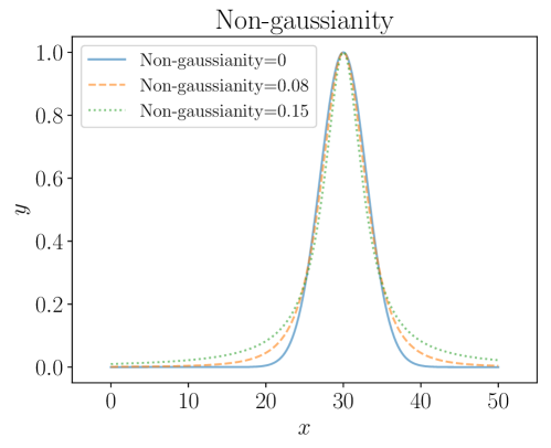
Figure 5: Examples of amorphous component shapes with different values for the nongaussianity.

where $C_{\rm m}$ is the measured crystallinity, and $C_{\rm pa}$ and $A_{\rm pa}$ are the integrated peak areas for the crystalline and amorphous components, respectively (see Figure 5 of Wall et al. (2014)). While its simplicity has made it advantageous, the calibration methodology has been limited in that the quality of the results largely depend on the ability of the user to manually assign backgrounds for count integration, resulting in potentially large inter-user variations. Although the point of the calibration curve is to reduce the inter-user variation, determinations still tend to be associated with moderate user error (3–5 vol %). As every user must independently practice background fittings using the calibration method, the results ultimately are only as good as the user’s ability to manually fit the data. This technique, while not constrained by a necessary library of diffraction patterns, also does not characterize the XRD properties of the amorphous material. This study presents a new approach using Bayesian inference to automate background determination for the calibration method, removing inter-user and intra-user biases in the determination of crystallinity and peak characteristics for amorphous/partially amorphous materials, regardless of what they are.

This paper is structured as follows. In Section 2, we outline the Bayesian framework of inference in general terms. In Section 3 we describe the specific modelling assumptions made by AMORPH, and Section 4 lists the probabilistic assumptions (i.e., the prior distributions) assumed by the program. Section 5 presents some example applications and comparisons with standard techniques, and finally we conclude in Section 6. Basic instructions for installation and use of AMORPH are given in A.

2 Bayesian inference

AMORPH is founded upon Bayesian inference (Gregory, 2005, O’Hagan and Forster, 2004, Sivia and Skilling, 2006), where probability distributions are used to model states of uncertainty about the values of unknown quantities. Bayesian inference is often implemented computationally with Markov Chain Monte Carlo (MCMC) methods (Mackay, 2003), and AMORPH is no exception. Loosely speaking, the goal is to fit a dataset with a model by exploring those regions of the model’s parameter space that are consistent with the data. The model assumptions are described in detail in Section 3, and the computation is performed with Diffusive Nested Sampling (an advanced MCMC method Brewer et al., 2011) as implemented in the software package DNest4 (Brewer and Foreman-Mackey, 2016). This method is robust to complicated posterior distributions.

There have been many approaches to problems of separating background from compact signals when noise is present, such as the famous CLEAN algorithm (Clark, 1980), through to more explicitly Bayesian approaches (e.g. Padayachee et al., 1999, Skilling, 1998, Harkness and Green, 2000, Hobson & McLachlan, 2003, Worpel & Schwope, 2015). AMORPH can be viewed as another case of this, with assumptions customized to this specific application.

Typically, one starts with the ‘prior distribution’ for unknown quantities (‘parameters’) $\boldsymbol{\theta}$, written $p(\boldsymbol{\theta}|I)$ (the probability distribution for $\boldsymbol{\theta}$ given prior information $I$). Throughout this paper, the bold $\boldsymbol{\theta}$ is used to denote a collection of unknown parameters, whereas $2\theta$ (with the factor of two, and the non-bold $\theta$) is later used to refer to the incident angle plus reflected angle, which is the standard notation in X-ray diffraction.

The prior describes an initial state of uncertainty about the parameter values, and is often a wide probability distribution. The prior is supplemented with $p(\boldsymbol{d}|\boldsymbol{\theta},I)$, sometimes called a ‘sampling distribution’, which describes the uncertainty about the data which we would have, if we knew the parameters (and the prior information), as a function of the parameters. The sampling distribution describes uncertainty about what data will be observed, but encodes some knowledge about the fact that the data have something to do with the parameters $\boldsymbol{\theta}$. For example, $p(\boldsymbol{d}|\boldsymbol{\theta},I)$ often encodes the assumption that the data has noise in it, and the specific noise values are unknown a priori.

The product of these two distributions is the joint prior

$$p(\boldsymbol{\theta},\boldsymbol{d}|I) =p(\boldsymbol{\theta}|I)p(\boldsymbol{d}|\boldsymbol{\theta},I)$$ (2)

which describes uncertainty about the value of both the parameters and the dataset. Once a specific observed dataset $\boldsymbol{d}_{\rm obs}$ is known, knowledge about $\boldsymbol{\theta}$ is updated from the prior $p(\boldsymbol{\theta}|I)$ to the posterior

$$p(\boldsymbol{\theta}|\boldsymbol{d}_{\rm obs},I) \propto p(\boldsymbol{\theta}|I)p(\boldsymbol{d}_{\rm obs}|\boldsymbol{\theta},I).$$ (3)

which takes the specific data $\boldsymbol{d}_{\rm obs}$ into account via conditioning. With the specific dataset, $p(\boldsymbol{d}_{\rm obs}|\boldsymbol{\theta},I)$ becomes a function of the unknown parameters $\boldsymbol{\theta}$ only and is called the likelihood function. The posterior distribution is therefore proportional to the prior distribution times the likelihood function.

When $\boldsymbol{\theta}$ is a large collection of parameters, the posterior distribution is a probability distribution over a high-dimensional parameter space. To represent it computationally, Markov Chain Monte Carlo (MCMC) methods are often used to generate samples from the parameter space, according to the posterior distribution. The output is a collection of plausible values of the parameters which can be used to approximate posterior probabilities. For example, the probability some parameter $\phi$ is greater than 3.4 is approximately the proportion of the posterior samples that have $\phi>3.4$. While many data analysis procedures work by finding the best fitting values of the parameters (i.e., a maximum likelihood estimate), Bayesian inference via MCMC involves exploring a range of plausible values for the parameters. Since AMORPH uses Diffusive Nested Sampling, it also calculates the ‘marginal likelihood’ or ‘evidence’ quantity $p(\boldsymbol{d}|I)$, which quantifies how well the model fits the data overall, averaged over all possible values of its parameters. This allows straightforward model comparison with any alternatives that may be proposed in the future (Skilling, 2006).

The computational cost of running AMORPH varies, as the posterior distribution depends on the data. The size of the dataset is important, of course. Another important factor is the number of MCMC samples desired. To quantify the uncertainty about a few scalar parameters, about 100 posterior samples is usually sufficient. Indeed, Mackay (2003, p. 380) suggests that only about twelve are needed for the uncertainty about a single quantity! However, if one wants to produce smooth histograms or look at details of the posterior distribution, many more samples are required.

On a modern desktop PC and using aggressive numerical settings (see A for details), some useful posterior samples can be obtained in about 15 minutes when the dataset contains about 1500 points. Typical analyses take approximately 5 hours to fully complete and yield a few hundred posterior samples. However, the complete runs presented in this paper took about a day each to run, as we ran with more conservative settings to ensure the number of posterior samples was about 1000 for each dataset.

3 The model curve

AMORPH fits the data with a model curve defined over some range from $x_{\rm min}$ to $x_{\rm max}$ (Fig. 1). Throughout this section, we use $x$ as a synonym for $2\theta$, since the problem is basically a curve-fitting problem where $x$ and $y$ are typically used.

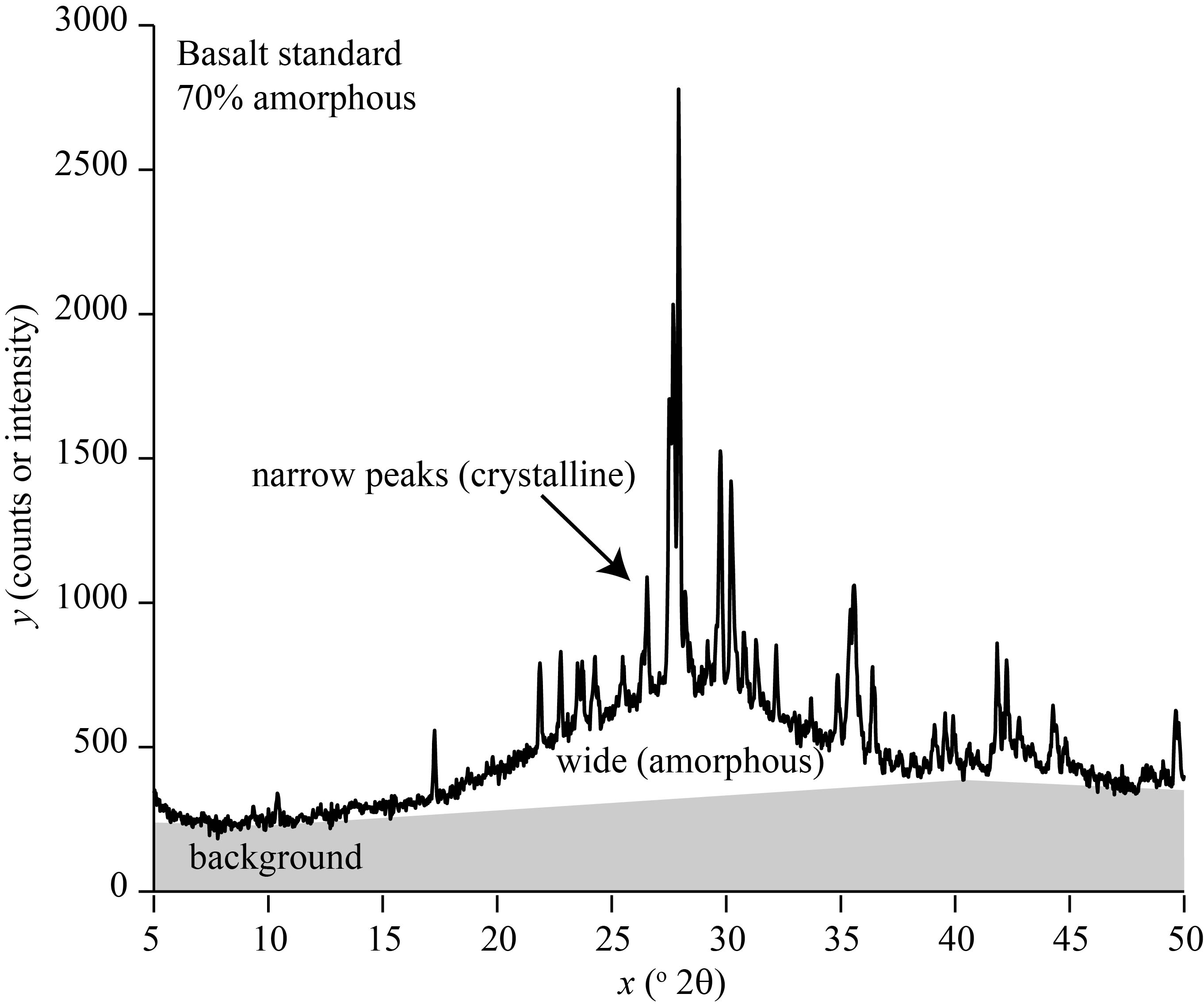
Figure 1: Powder X-ray diffraction results for a basalt standard with 70% amorphous material. Annotation corresponds to the model components: background, amorphous (wide) component, and crystalline component (narrow peaks).

The model curve is a function $y=f(x;\boldsymbol{\theta})$, which is assumed to be a sum of the following components identified in Figure 1:

1. A background component, described by parameters $\boldsymbol{\theta}_{\rm bg}$

2. An amorphous component, described by parameters $\boldsymbol{\theta}_{\rm amorph}$

3. A crystalline component, described by parameters $\boldsymbol{\theta}_{\rm xtal}$

The total model function $f_{\rm tot}(x)$ is therefore

$$f_{\rm tot}(x) =f_{\rm bg}(x;\boldsymbol{\theta}_{\rm bg})+f_{\rm amorph}(x;\boldsymbol{\theta}_{\rm amorph})+f_{\rm xtal}(x;\boldsymbol{\theta}_{\rm xtal})$$ (4)

and the measured amorphous content ($A_{\rm m}$ or $1-C_{\rm m}$) is defined, similar to Equation 1, as the proportion of the area in the amorphous and crystalline components which is accounted for by the amorphous component:

$${A_{\rm m}=1-C_{\rm m}} =\frac{\int_{x_{\rm min}}^{x_{\rm max}}f_{\rm amorph}(x;\boldsymbol{\theta}_{\rm amorph})\,dx}{\int_{x_{\rm min}}^{x_{\rm max}}f_{\rm amorph}(x;\boldsymbol{\theta}_{\rm amorph})\,dx+\int_{x_{\rm min}}^{x_{\rm max}}f_{\rm xtal}(x;\boldsymbol{\theta}_{\rm xtal})\,dx}$$ (5)

From each sample from the posterior distribution for all of the parameters, it is straightforward to compute the proportion of amorphous material, and hence calculate the marginal posterior distribution of the amorphous content. In the following subsections, we describe the specific parameterizations of the three parts of the model curve, that is, the functional forms of $f_{\rm bg}$, $f_{\rm amorph}$, and $f_{\rm xtal}$.

3.1 The background component

The background component is assumed to be piecewise linear, with constant slope between $x=x_{\rm min}$ and $x=10$°, between $x=10$° and $x=40$°, and between $x=40$° and $x=x_{\rm max}$. These values are selected to maintain a linear background over the interval from 10–40°, the predominant range of amorphous materials (8.8 – 2.25 Å) analyzed using a Cu K$\alpha$ x-ray source (Table 1), while still allowing for some flexibility in the structure of the background outside this range.

We parameterized the background component using five parameters. Firstly, there is a mean level $b$, which sets the typical amplitude of the background component. There are also four parameters $n_{1},...,n_{4}$, which determine the offset of four ‘control points’ from the mean level. The positions of the four control points are then:

$$\left(x_{\rm min},be^{n_{1}}\right)$$

$$\left(10,be^{n_{2}}\right)$$

$$\left(40,be^{n_{3}}\right)$$

$$\left(x_{\rm max},be^{n_{4}}\right).$$

Control points may be set by the user, as it may depend on the X-ray source in use and changes in the required range for the linear background as a function of the nature of the amorphous material (Table 1). The value of the background component at any other point is found by linear interpolation of these control points. Figure 2 shows three example background curves generated from this parameterization, with typical values of the parameters.

X-ray Anode	X-ray wavelength	Control point 2	Control point 3
	(Å)	(°$2\theta$)	(°$2\theta$)
Cr	2.29	15.0	61.2
Fe	1.94	12.7	51.1
Co	1.79	11.7	46.9
Cu	1.54	10.0	40.0
Mo	0.71	4.6	18.2
Ag	0.56	3.6	14.3

Table 1: Typical XRD anodes with recommended background control points based on a predominant 8.8–2.25 Å amorphous peak.

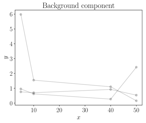
Figure 2: Three example functions showing possible shapes of the background component.

3.2 The crystalline component

We assume that there is some number $N_{\rm xtal}$ of narrow peaks due to crystalline material, each of which has the same shape. The shapes of the narrow peaks are controlled by a single shape parameter $\nu_{\rm xtal}$, assumed common to all of the narrow peaks. The chosen shape is based on the Student’s $t$-distribution, which allows the peaks to be heavy-tailed if $\nu_{\rm xtal}$ is low, and to be Lorentzian or Cauchy in shape if $\nu_{\rm xtal}$ is exactly 1. As $\nu_{\rm xtal}$ is high, the shape approximates a gaussian.

The $i$th peak is parameterized by its central position $X_{i,\rm xtal}$, total integrated ‘mass’ $M_{i,\rm xtal}$, and width $W_{i,\rm xtal}$. The parameter vector for crystalline component is

$$\boldsymbol{\theta}_{\rm xtal} =\{N_{\rm xtal},\nu_{\rm xtal},X_{1,\rm xtal},...,X_{N,\rm xtal},M_{1,\rm xtal},...,M_{N,\rm xtal},W_{1,\rm xtal},...,W_{N,\rm xtal}\}$$ (6)

and the total shape contributed by the crystalline component is a sum of the $N_{\rm xtal}$ peaks:

$$f_{\rm xtal}(x;\boldsymbol{\theta}_{\rm xtal}) =\frac{\Gamma(\frac{\nu_{\rm xtal}+1}{2})}{\sqrt{\nu_{\rm xtal}\pi}\Gamma(\frac{\nu_{\rm xtal}}{2})}\sum_{i=1}^{N_{\rm xtal}}\frac{M_{i,\rm xtal}}{W_{i,\rm xtal}}\left(1+\frac{1}{\nu}\left(\frac{x-X_{i,\rm xtal}}{W_{i,\rm xtal}}\right)^{2}\right)^{-\frac{\nu_{\rm xtal}+1}{2}}.$$ (7)

The terms inside the sum have the form of the probability density function of the $t$-distribution, adjusted by shifting according to the central position and widening by the width, and the total integral is scaled by the mass parameters. $\Gamma()$ is the gamma function.

For computational efficiency, evaluation of Equation 7 is performed using a lookup table. In addition, we evaluate the peak shapes at the $x$-position of each data point, rather than integrating the peak shape across a finite bin width. This is faster but must be kept in mind when interpreting parameters affected by this assumption, such as the widths of the narrow peaks.

3.3 The amorphous component

The amorphous component is also composed of a sum of peaks, which we chose to be gaussians. The parameterization is the same as for the crystalline peaks but with a fixed, high value for the shape parameter. Apart from the gaussian shape, the only other difference is the prior distributions for the positions, masses, and widths, given in Section 4. In short, the wide gaussians representing the amorphous component are more likely to be located near the middle of the dataset, and to be wider. The constrainted prior for the positions of the wide amorphous peaks prevents the program from attempting to explain background variations near the edge of the data using the amorphous component.

There is some number $N_{\rm amorph}$ of gaussians in the amorphous component. The $i$th gaussian is parameterized by its central position $X_{i,\rm amorph}$, mass (total integral) $M_{i,\rm amorph}$, and width $W_{i,\rm amorph}$. The parameter vector for the wide gaussians is

$$\boldsymbol{\theta}_{\rm amorph}=\{N_{\rm amorph},X_{1,\rm amorph},...,X_{N,\rm amorph},M_{1,\rm amorph},...,M_{N,\rm amorph},$$ (8)

$$\quad\quad W_{1,\rm amorph},...,W_{N,\rm amorph}\}$$ (9)

and the total shape contributed by the amorphous component is a sum of the $N_{\rm amorph}$ gaussians:

$$f_{\rm amorph}(x;\boldsymbol{\theta}_{\rm amorph}) =\frac{1}{\sqrt{2\pi}}\sum_{i=1}^{N_{\rm amorph}}\frac{M_{i,\rm amorph}}{W_{i,\rm amorph}}\exp\left[-\frac{1}{2W_{i,\rm amorph}^{2}}\left(x-X_{i,\rm amorph}\right)^{2}\right].$$ (10)

Figure 3 shows several examples of possible amorphous component shapes. The prior distributions (specified in Section 4) constrain the central positions of these gaussians much more strongly than the central positions of the narrow peaks (crystalline component). AMORPH is primarily able to distinguish the crystalline and amorphous components due to the different priors for the widths of the two different sets of peaks.

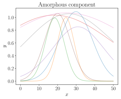
Figure 3: Some examples of plausible shapes for the amorphous component, generated from the prior distribution for its parameters (Section 4). For visual purposes only, these were scaled to amplitudes $\sim$ 1.

3.4 Derived properties

Some derived properties of the amorphous component can be used to summarize its shape. We have included the ‘width’ (second central moment, analogous to the standard deviation), ‘skewness’, which describes asymmetry, and ‘nongaussianity’ which quantifies the departure from gaussianity. These are not the same concept, as the amorphous component could be non-gaussian while still being symmetric (and thus having zero skewness).

Defining a normalized version of the amorphous component as

$$g(x) =\frac{f_{\rm amorph}(x)}{\int_{-\infty}^{\infty}f_{\rm amorph}(x^{\prime})\,dx^{\prime}},$$ (11)

its center of mass is

center $$=\int_{-\infty}^{\infty}xg(x)\,dx.$$ (12)

The width of the amorphous component (its second central moment, perhaps better interpreted as a half-width) is defined by

width $$=\sqrt{\int_{-\infty}^{\infty}g(x)\left(x-\textnormal{center}\right)^{2}\,dx},$$ (13)

and the skewness is

skewness $$=\int_{-\infty}^{\infty}g(x)\left(\frac{x-\textnormal{center}}{\textnormal{width}}\right)^{3}\,dx.$$ (14)

To quantify the non-gaussianity, we construct a gaussian $g^{\prime}(x)$ with the same centre, width, and total integral as $g(x)$, and compute the Kullback-Leibler divergence from $g^{\prime}$ to $g$:

non-gaussianity $$=\int_{-\infty}^{\infty}g(x)\log\left[\frac{g(x)}{g^{\prime}(x)}\right]\,dx.$$ (15)

where

$$g^{\prime}(x) =\frac{1}{\textnormal{width}\times\sqrt{2\pi}}\exp\left[-\frac{1}{2\times(\textnormal{width})^{2}}\left(x-\textnormal{center}\right)^{2}\right].$$ (16)

The Kullback-Leibler divergence is a standard way of quantifying how different one ‘measure’ ($\equiv$ density function, for our purposes here) is from another (Knuth and Skilling, 2012). It is zero when the two measures are the same, in our case, if $g(x)$ is a gaussian. See Figures 4 and 5 for example shapes for the amorphous component, and corresponding values of the skewness and nongaussianity.

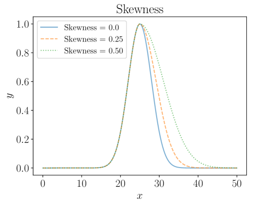
Figure 4: Examples of amorphous component shapes with different values for the skewness.

4 Prior probability distributions

The joint prior distribution for all of the unknown parameters and the data must be specified. When the number of parameters is large, this is often done hierarchically, by specifying the priors conditional on some ‘hyperparameters’, and then assigning priors to the hyperparameters.

In these cases, the joint prior distribution for the hyperparameters $\boldsymbol{\alpha}$, parameters, and data, is written $p(\boldsymbol{\alpha},\boldsymbol{\theta},\boldsymbol{d}|I)$, and is usually factorized in this way:

$$p(\boldsymbol{\alpha},\boldsymbol{\theta},\boldsymbol{d}|I) =p(\boldsymbol{\alpha}|I)p(\boldsymbol{\theta}|\boldsymbol{\alpha},I)p(\boldsymbol{d}|\boldsymbol{\theta},\boldsymbol{\alpha},I)$$ (17)

$$=p(\boldsymbol{\alpha}|I)p(\boldsymbol{\theta}|\boldsymbol{\alpha},I)p(\boldsymbol{d}|\boldsymbol{\theta},I)$$ (18)

where the first step is true in general by the product rule of probability, and the second step assumes that knowing the parameters would make the hyperparameters irrelevant when predicting what data would be observed. In the AMORPH model, we introduced hyperparameters describing the typical integrated area (‘mass’) and width of the peaks for the amorphous component, and the degree to which the actual masses and widths are scattered around that typical value. This was also done for the crystalline component.

A directed acyclic graph, also known as a probabilistic graphical model (PGM), which depicts the dependence structure of the entire joint prior probability distribution, is shown in Figure 6. The prior distributions themselves are specified in Table 2.

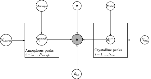
Figure 6: The PGM. The hyperparameters controlling the prior distributions for the amorphous and crystalline peaks are denoted collectively by $\boldsymbol{\alpha}_{\rm amorph}$ and $\boldsymbol{\alpha}_{\rm xtal}$ respectively. The noise-related parameters are collected under $\boldsymbol{\sigma}$. The data is $\boldsymbol{y}$.

Quantity	Meaning	Prior distribution
Prior information
$n$	Number of measurements	given
$\{x_{1},x_{2},...,x_{n}\}$	$x$-values of measurements	given
$x_{\rm range}$	Range of measurements	$\max(x_{1},...,x_{n})-\min(x_{1},...,x_{n})$
Hyperparameters
$N_{\rm xtal}$	Number of narrow peaks	$\propto 1/(N_{\rm xtal}+1)$, $N_{\rm xtal}\in\{0,1,...,1000\}$
$N_{\rm amorph}$	Number of wide peaks	$\propto 1/(N_{\rm amorph}+1)$, $N_{\rm amorph}\in\{0,1,...,1000\}$
$a_{\ln M,\rm xtal}$	Typical log-mass of narrow peaks	Laplace(0, 5)
$a_{\ln M,\rm amorph}$	Typical log-mass of wide peaks	Laplace(0, 5)
$b_{\ln M,\rm xtal}$	Diversity of log-mass of narrow peaks	Uniform(0, 5)
$b_{\ln M,\rm amorph}$	Diversity of log-mass of wide peaks	Uniform(0, 5)
$a_{\ln W,\rm xtal}$	Typical log-width of narrow peaks	LogUniform$(10^{-3}x_{\rm range},0.05x_{\rm range})$
$a_{\ln W,\rm amorph}$	Typical log-width of wide peaks	LogUniform$(0.05x_{\rm range},x_{\rm range})$
$b_{\ln W,\rm xtal}$	Diversity of log-width of narrow peaks	Uniform(0, 0.1)
$b_{\ln W,\rm amorph}$	Diversity of log-width of wide peaks	Uniform(0, 0.2)
Background parameters
$b$	Mean background level	$\ln b\sim$ Laplace$(0,5)$
$\{n_{1},...,n_{4}\}$	Background deviations	independent Normal$(0,1)$
Crystalline parameters
$X_{i,\rm xtal}$	Positions of narrow peaks	Uniform$(x_{\rm min},x_{\rm max})$
$M_{i,\rm xtal}$	Masses of narrow peaks	$\ln M_{i,\rm xtal}\sim\textnormal{Laplace}\left(a_{\ln M,\rm xtal},b_{\ln M,\rm xtal}\right)$
$W_{i,\rm xtal}$	Widths of narrow peaks	$\ln W_{i,\rm xtal}\sim\textnormal{Laplace}\left(a_{\ln W,\rm xtal},b_{\ln W,\rm xtal}\right)$
$\nu_{\rm xtal}$	Shape of narrow peaks (common)	LogUniform$(0.1,100)$
Amorphous parameters
$X_{i,\rm amorph}$	Positions of wide peaks	Uniform$(x_{\rm min}+0.3x_{\rm range},x_{\rm max}-0.3x_{\rm range})$
$M_{i,\rm amorph}$	Masses of wide peaks	$\ln M_{i,\rm amorph}\sim\textnormal{Laplace}\left(a_{\ln M,\rm amorph},b_{\ln M,\rm amorph}\right)$
$W_{i,\rm amorph}$	Widths of wide peaks	$\ln W_{i,\rm amorph}\sim\textnormal{Laplace}\left(a_{\ln W,\rm amorph},b_{\ln W,\rm amorph}\right)$
Noise parameters
$\sigma_{0}$	Constant noise level	$\ln\sigma_{0}\sim\textnormal{Laplace}(0,5)$
$\sigma_{1}$	Noise proportional to $\sqrt{\textnormal{model}}$	$\ln\sigma_{1}\sim\textnormal{Laplace}(0,5)$
$\nu$	Shape parameter for $t$-distribution	LogUniform$(1,1000)$
	for noise
Data
$\{y_{1},y_{2},...,y_{n}\}$	Measurements	independent
		Student-$t\left(f(x_{i};\boldsymbol{\theta}),\sqrt{\sigma_{0}^{2}+\sigma_{1}f(x_{i};\boldsymbol{\theta})},\nu\right)$

Table 2: The prior distributions for all hyperparameters, parameters, and the data.

Most of the chosen distributions were intended to be reasonably conservative and wide, but not excessively so. Some of the prior distributions in AMORPH use the log-uniform distribution, sometimes (erroneously) called a Jeffreys prior, whose density for a quantity $z$ is proportional to $1/z$. This prior is equivalent to a uniform prior for the logarithm of the quantity, and encodes the fact that the order of magnitude of a positive quantity may be unknown.

We used a Laplace distribution for some informative priors, rather than a more conventional normal distribution, because it assigns higher prior probability to values far from the center (compared to a normal distribution), and can be computed conveniently. Specifically, special functions such as the inverse of the error function are needed. The Laplace distribution with location parameter (central position) $a$ and scale parameter (width) $b$ has probability density given by

$$p(x|a,b) =\frac{1}{2b}\exp\left[-\frac{|x-a|}{b}\right].$$ (19)

The priors for the positions and widths of the ‘amorphous’ and ‘crystalline’ peaks are different, to account for the prior knowledge that they should result in wide peaks near the centre of the domain, and narrow peaks throughout the domain respectively.

The prior for the data given all the parameters (i.e., the sampling distribution) is a student-$t$ distribution, centered at the model curve $f(x;\boldsymbol{\theta})$. The $t$ distribution allows for potentially heavier tails than a normal distribution would. Thus, analyses with AMORPH should be able to cope with discrepant datapoints as long as they are not locally correlated (which would cause them to be mistaken for peaks).

AMORPH does not assume a known number of peaks for either the amorphous or the crystalline component — the appropriate number of peaks is inferred from the data. The maximum number of peaks for each component is set to 1000.

5 Applications

5.1 Crystallinity

To date, applications of crystallinity determinations via XRD methodologies on terrestrial samples have primarily focused on volcanic materials (e.g., Wall et al., 2014, Ellis et al., 2015, Andrade et al., 2017, Zorn et al., 2018), linking crystallinity of volcanic glass to timescales of geologic processes. The primary advantage of this technique being its ability to determine crystallinities for finer grain sizes than typically possible through standard petrologic techniques (Rowe et al., 2012). In contrast, planetary science usages for determining crystallinity have largely focused on quantification of the amorphous and crystalline components for mass balance determination of physical and chemical components in diverse geologic materials (e.g., Blake et al., 2013, Dehouck et al., 2014).

The AMORPH program calculates a fraction of amorphous material ($A_{\rm m}$) for each posterior sample of the parameters using Equation 5. Thus, measured crystallinity ($C_{\rm m}$) is easily determined from the relationship $C_{\rm m}=1-A_{\rm m}$. To test the applicability of AMORPH crystallinity results, we have analysed the Mars Scientific Laboratory (MSL) CheMin instrument X-ray diffraction patterns of loose basaltic sand from the Bagnold Sand Dunes (Gobabeb; Achilles et al., 2017, Lapotre et al., 2017) and sediments drilled from a silicic mudstone (Buckskin sample; Morris et al., 2016), both which have significant amorphous materials (CheMin instrument data). CheMin diffraction patterns have been processed using the original Co K$\alpha$ ($1.7890$ Å) data as well as data transformed from a Co K$\alpha$ to Cu K$\alpha$ ($1.5406$ Å) X-ray source using Bragg’s law. This recalculation simply allows for an easier visual comparison to terrestrial samples analysed with the more standard Cu K$\alpha$ X-ray source (see below). Note that for Co K$\alpha$ results, background critical points have been adjusted to 11.7–46.9° $2\theta$ to maintain the linear background over the amorphous region from $\sim$ 8.8 to 2.25 Å(Table  1). Although the results are uncalibrated, measured crystallinites provide a good first approximation of actual crystallinity, and relative differences are robust. Measured amorphous content of the Gobabeb 2 sample is 36.7 $\pm$ 2.9$\%$ (63.3$\%$ crystallinity) while the Buckskin 2 sediment contains 45.3 $\pm$ 2.9$\%$ amorphous phases (54.7 $\%$ crystallinity; Fig. 7). Comparatively, published FULLPAT calculations of amorphous contents are  35 $\pm$ 15$\%$ for Gobabeb and 50 $\pm$ 15$\%$ for Buckskin (Achilles et al., 2017, Morris et al., 2016).

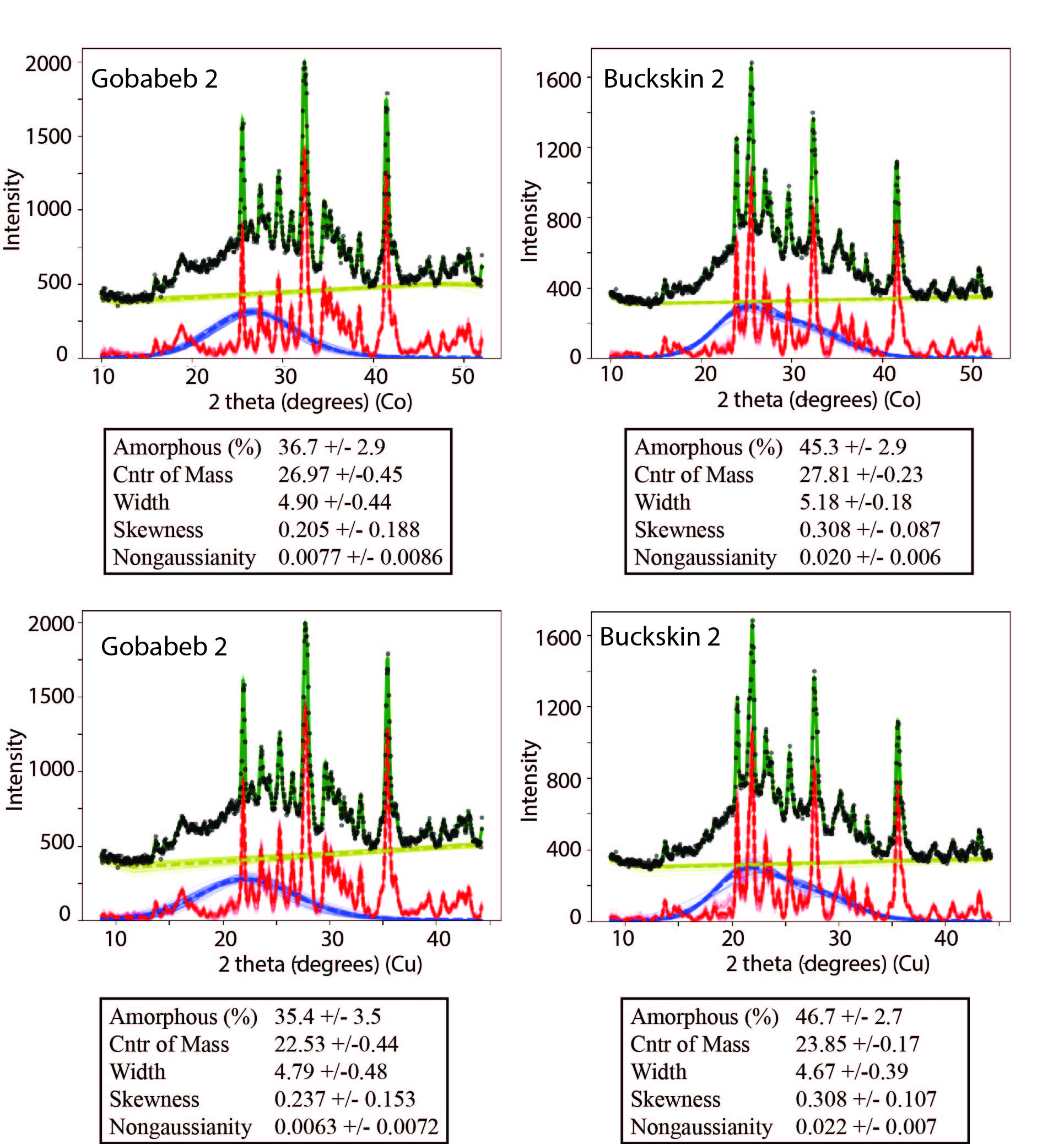
Figure 7: Analysis of Gobabeb 2 (left) and Buckskin 2 (right) results from the CheMin instrument on the MSL Curiosity rover (data sourced as above). Upper panels illustrate initial Co K$\alpha$ processed results while lower panels show AMORPH results after translating data to a Cu K$\alpha$ source (see text for details). Thin solid lines represent individual model results for crystalline (red) and amorphous (blue) components, linear backgrounds (yellow), and compiled model results (green). Bold dashed lines (same colors as individual model results) indicate average model results. Calculated statistics provided by AMORPH for each analysis are indicated below the model results.

The measured crystallinity is not equivalent to an “actual” or “true” crystallinity, although the values are often very close to one another as noted above. Therefore, this procedure does not negate the need for calibration standards to translate measured crystallinity to an actual crystallinity. Calibration standards can be easily created by mixing powdered minerals (e.g. olivine, pyroxene, plagioclase) with powdered glass in known proportions to simulate volcanic material of varying crystallinities (e.g., Rowe et al., 2012, Wall et al., 2014).

Transmission and absorption of X-rays in the material will vary as the ratio of mineral to glass changes in the sample, causing a deviation from a 1:1 line (Fig. 8). In addition to theoretical considerations, practical challenges also exist for background fitting. At low crystallinity ($\lesssim 10\%$) diffraction patterns are dominated by the low amplitude amorphous peak such that removing the effects of background noise becomes problematic, resulting in overestimated crystallinities. At high crystallinity ($\gtrsim 90\%$) the problem arises that peak overlaps in multi-mineral assemblages cause apparent broadening effects, and may be subsequently modeled as “amorphous” and thus crystallinities underestimated. The calibration curve therefore is utilized to remove these effects. This is also an important step as different X-ray diffractometers will provide slightly different calibration curves (Fig. 8). Differences between instruments largely reflect changes in background intensity and shape, particularly at low values of $2\theta$.

Since the wide peak for many amorphous materials does not extend appreciably out of the range from 10–40° $2\theta$ (for a Cu K$\alpha$ source), peak area integration outside of this range will decrease proportionally the relative contribution of the amorphous material (only peaks for crystalline materials are outside this range in the example depicted in Figure 9, with the corresponding fitting residuals and the posterior distributions for the number of narrow peaks in Figure 10 and Figure 11, respectively). It should be noted of course that this only effects the measured crystallinity and as long as the calibration standards are processed under the same conditions as the unknown, the “actual” crystallinity is not significantly affected by the choice in selected analysis interval. Results of the AMORPH calculations show good agreement to calibration curves using the manual calibration approach for the same set of standards analyzed on the same PANalytical Empyrean X-ray diffractometer (Fig. 12).

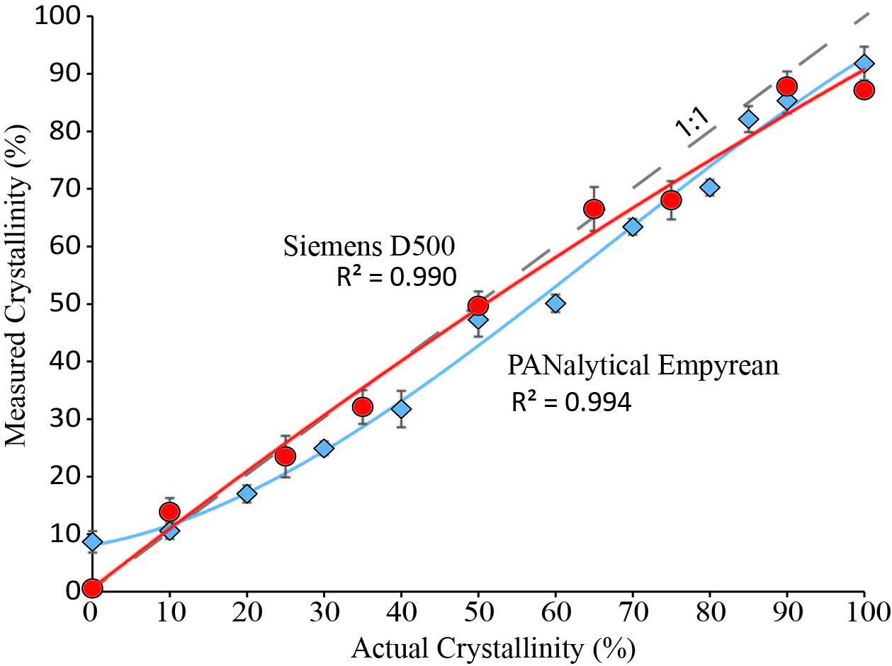
Figure 8: Two calibration curves of the same standard material (rhyolite) are compared from different instrumentation, including a Siemens D500 (Washington State University; red circles) and a PANalytical Empyrean (University of Auckland; blue diamonds).

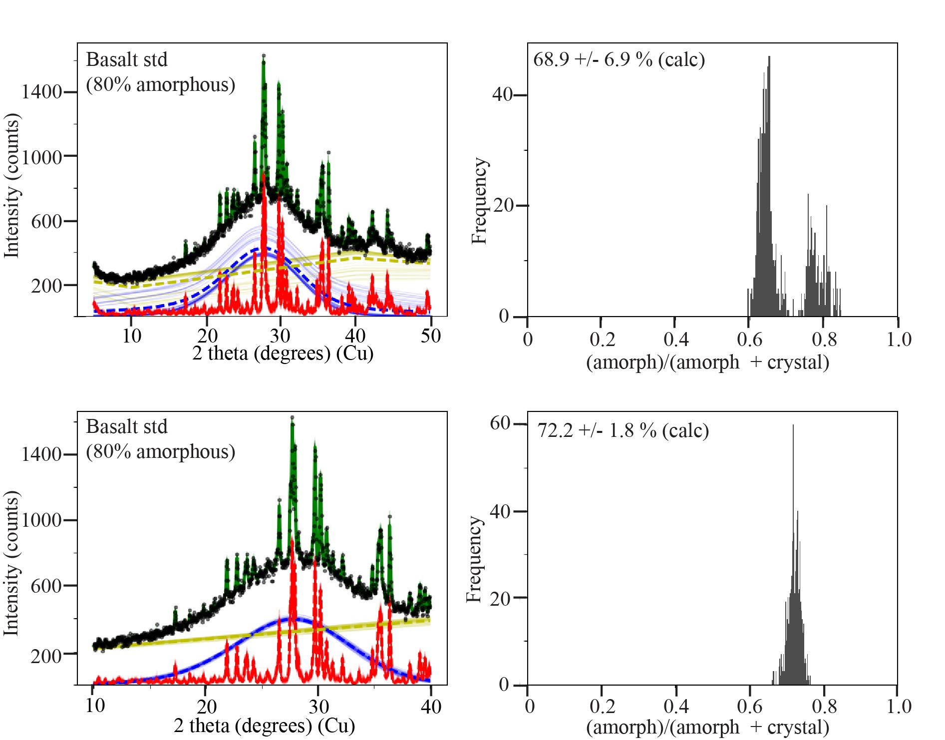
Figure 9: Model results for a basalt standard containing 80% amorphous glass. Data was processed from 5–50° $2\theta$ (upper left panel) with a calculated amorphous content of 68.9% (upper right panel). The same data was processed instead from 10–40° $2\theta$ (lower left panel) with a calculated amorphous content of 72.2% (lower right panel). Line colors same as in Figure 7. The reasons for the differences are discussed in the text.

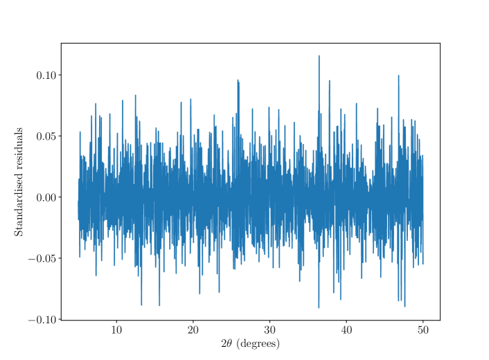
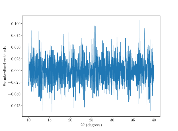
Figure 10: Residuals of the model fits shown in Figure 9, showing that the features of the data have been captured (upper panel is 5–50° $2\theta$; lower panel is 10–40° $2\theta$ dataset). Technically, there is no single set of residuals, but a posterior distribution over them, represented by the residuals of each curve in the generated sample. Therefore, these plots show the residuals of the posterior mean model curve.

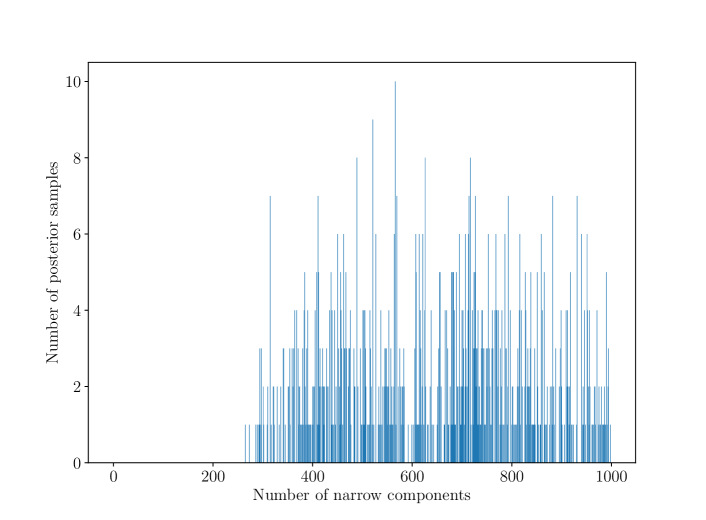
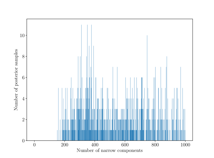
Figure 11: Posterior distributions for the number of narrow peaks for the fits shown in Figure 9 (upper panel is 5–50° $2\theta$; lower panel is 10–40° $2\theta$ dataset). A minimum number of peaks is required in both cases, but the data cannot rule out large numbers of peaks (of very small amplitude). There are more peaks in the 5–50°case.

For some materials, e.g. allophane, the amorphous region extends beyond the 10–40° $2\theta$ range and thus would require analysis over a larger $2\theta$ interval. The trade-off in extending the $2\theta$ range is increased processing time and further deviation from a 1:1 calibration line. Since the analysis time is, in part, a function of the number of data points, if greater range in $2\theta$ is required, decreasing the total number of points (larger step size during analysis or manual removal of points in $2\theta$ regions not of interest) will offset additional analysis time. Thus we recommend that the optimal range for data processing in terms of time and accuracy is from 8.8 to 2.2 Å or 10–40° $2\theta$ for a Cu K$\alpha$ X-ray source (see Table 1 for other X-ray sources) for crystallinity measurements of most volcanics. Importantly, reducing the data range from 5–50° $2\theta$ to 10–40° $2\theta$, does not increase the error associated with the peak fitting computational process with respect to other sources of error in sample selection and processing. In fact, for some analyses the variance in calculated crystallinity is appreciably reduced by shortening the range in analysed $2\theta$ and thereby reducing potential error associated with modeling background positions (Fig  9).

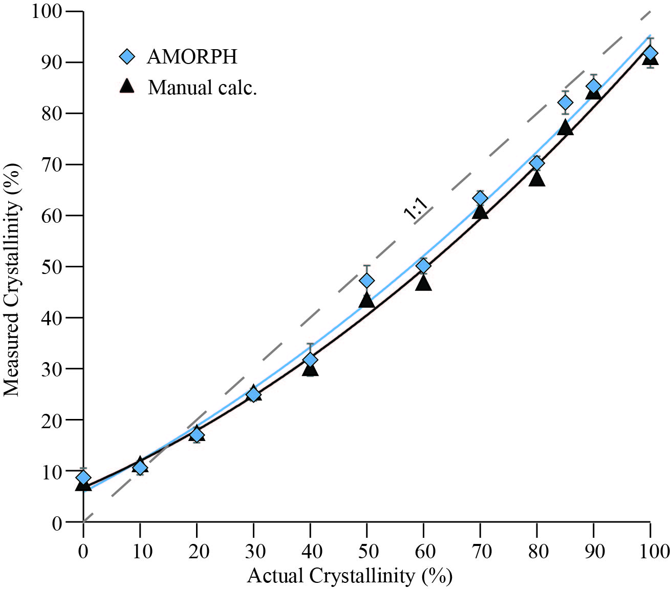
Figure 12: Comparison of calibration results for rhyolite calculated from AMORPH compared to a calibration calculated using the manual procedure described by Rowe et al. (2012).

5.2 Amorphous Characteristics

As discussed above, one of the primary advantages of the AMORPH program is that it can independently model characteristics of the amorphous component. In particular, centre of mass, skewness, and nongaussianity are distinctive amongst different amorphous materials. In contrast to crystallinity determinations, the focus of applications looking at the characteristics of the amorphous material are for indentification of the amorphous phase(s) (e.g., Dehouck et al., 2014). To test the ability of AMORPH to characterise amorphous phases, we present amorphous characteristics of rhyolite and basalt glass picked from a Taupo pumice (73.5 wt% SiO₂; P2166C; Barker et al., 2015) and a Kilauea basalt (51 wt% SiO₂; KS08-108E; Wooten et al., 2009, Rowe et al., 2015), respectively. The most notable differences in the amorphous component characteristics calculated for diffraction patterns for basalt and rhyolite glass include a positive skewness and shift to lower centre of mass $2\theta$ values for the rhyolite glass compared to the basalt glass (Fig 13).

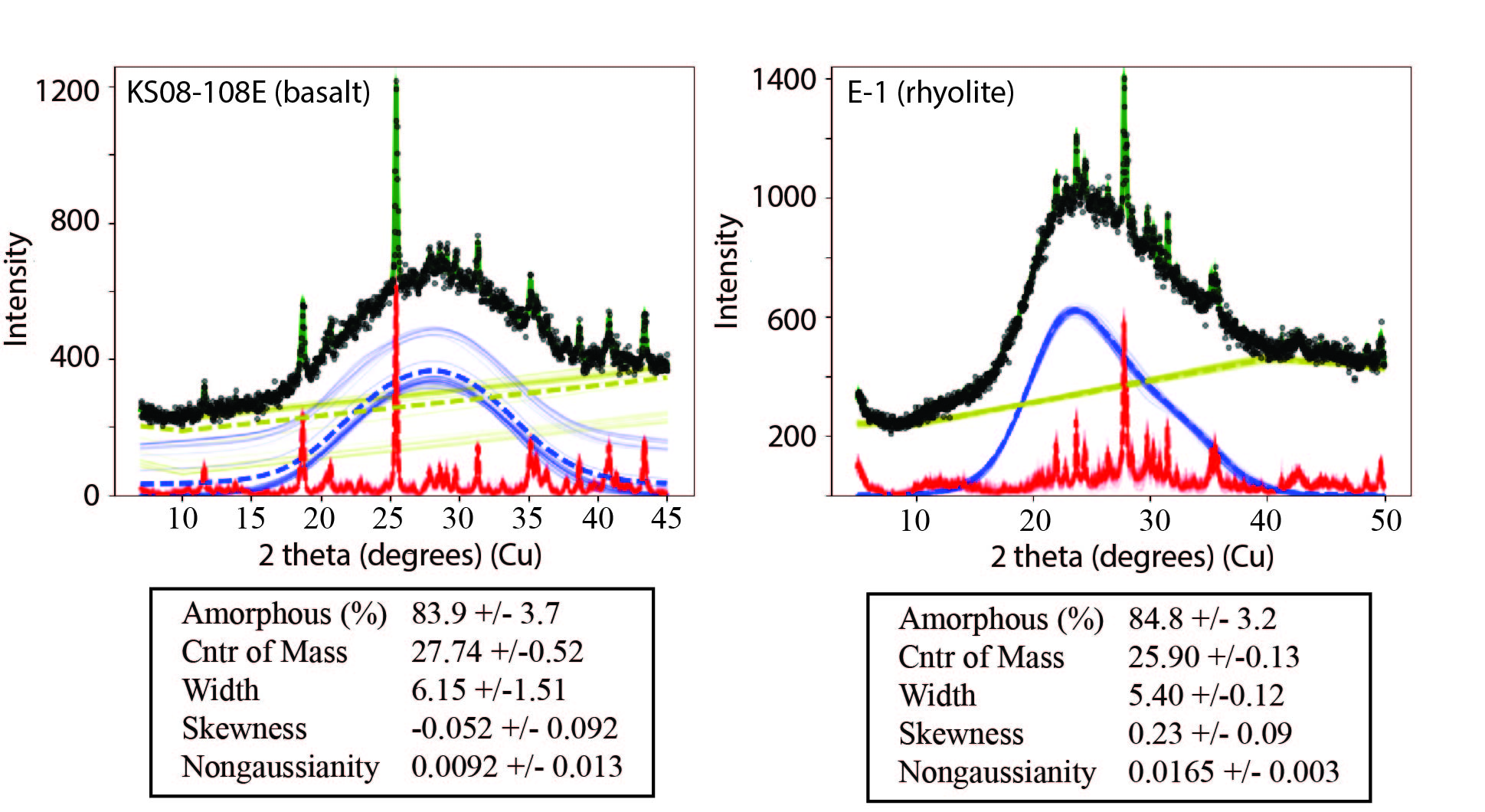
Figure 13: Examples of changing characteristics of amorphous material based on composition. Kilauea basalt glass (left) and taupo rhyolite glass (right) were analyzed on a PANalytical Empyrean XRD at University of Auckland. Calculated statistics for each analysis are provided below the model results. Line colors same as described in Figure 7. Note in particular the change in skewness from basalt to rhyolite.

Although CheMin diffraction analyses were run on a different X-ray diffractometer from the terrestrial samples shown here, similar relative changes in amorphous characteristics can be observed in X-ray diffraction data from Mars (Fig  7). It is unknown if/how the X-ray source (e.g. Cu versus Co) fundamentally changes the peak shape characteristics of the amorphous content in this study. However, qualitative assessment suggests similar overall peak shapes between terrestrial samples analysed with a Cu X-ray anode (Fig. 13) and those analysed with a Co X-ray anode (Fig. 7). In particular, the Buckskin 2 analysis of the amorphous component indicates a greater positive skewness than the Gobabeb 2 sample. In addition, the nongaussianity of the Buckskin 2 sample is $\sim 3\times$ greater compared to the Gobabeb 2 amorphous component. These results suggest a change in the composition of the amorphous material between the two Martian samples. This interpretation, is consistent with prior published results which suggest that at the Gobabeb locality (Namib Dune, Bagnold Dune Field), the sample is dominated by a basaltic mineralogy, while at the Buckskin locality, the amorphous component has been calculated to contain  77 wt% SiO₂ (i.e. rhyolitic; Morris et al., 2016, Achilles et al., 2017).

While results may imply a qualitative relationship to composition, further testing and an understanding of the program’s limitations is necessary to better quantify compositional correlations. In particular, the AMORPH program can quantify the peak shape and proportion of amorphous material but it cannot deconvolve the diffraction pattern of multiple amorphous phases, nor can it distinguish between non-crystalline materials and X-ray amorphous phases such as nanophase oxides (Blake et al., 2013).

6 Conclusions

The AMORPH program’s statistical approach to interpreting amorphous materials in X-ray diffraction patterns provides a new and unique methodology. By explicitly specifying a set of assumptions and computing their implications, we can automatically produce outputs separating the amorphous and crystalline components and quantifying their properties, along with a corresponding uncertainty estimate for any inferred quantity. A significant outcome of this research is that it reduces intra- and inter-user variability by eliminating the need for manual background fitting, the largest source of error in the calibration methodology for quantifying the amorphous component. Results demonstrate that this approach 1) accurately reproduces values of known crystallinity and 2) is consistent with prior manual approaches to the calibration method. Quantification of the amorphous content however still requires a calibration curve to correct for x-ray absorption/emission in heterogeneous materials, and to remove systematic biases in both background fitting and instrumentation.

In addition to the quantification of amorphous and crystalline components, the AMORPH program calculates statistical parameters of the amorphous component, including the centre of mass, width of amorphous component, skewness, and nongaussianity. Characterization of the amorphous component requires no calibration and outputs show clear distinctions, in particular in terms of skewness, as a function of changing composition of the amorphous material in the demonstrated examples of geologic materials from Earth and Mars.

References

Appendix A Installation and usage

The entire repository, including C++ and Python source code, and a precompiled executable file for Microsoft Windows, is hosted on Bitbucket at the following URL:

https://bitbucket.org/eggplantbren/amorph

AMORPH is free software, released under the terms of the GNU General Public Licence, version 3. For most users, we suggest simply using the pre-compiled Windows executable AMORPH.exe from the repository. Before executing the program, open config.yaml in a text editor to set up the run. This file contains all the information about the run, such as the name of the file containing the data. Then run AMORPH.exe. All files to be processed by AMORPH need to be in .txt file format, space delimited, with no headers. For simplicity, text files for processing should be located in the same folder as the AMORPH.exe program.

The configuration file lets you control the data being analyzed, and various options such as the number of simultaneous threads to run. You can also choose to use either OPTIONS_AGGRESSIVE or OPTIONS (or your own file), which contain parameter settings for DNest4. OPTIONS is more conservative than OPTIONS_AGGRESSIVE, as the names suggest.

The program is set to run until 10,000 saved parameter sets (‘particles’) have been generated. Data outputs may be viewed at any point, however, closing the program before reaching 10,000 will reduce the accuracy of the final calculations. After running for a while, the output can be viewed by running the Python script showresults.py:

python3 showresults.py

This script makes use of the packages Numpy and matplotlib, and has only been tested under Python 3. Anaconda is a convenient distribution of Python which comes with scientific packages pre-installed. Since AMORPH is really just a specific data analysis situation implemented for DNest4 (Brewer and Foreman-Mackey, 2016), that paper provides much more detail about AMORPH’s output and further available options.

References

- Achilles et al. (2017) Achilles, C.N., et al. 2017. Mineralogy of an active eolian sediment from the Namib Dune, Gale Crater, Mars. Journal of Geophysical Research Planets, 122(11), 2344-2361, doi: 10.1002/2017JE005262.
- Achilles et al. (2013) Achilles, C.N., Morris, R.V., Chipera, S.J., Ming, D.W., & Rampe, E.B. 2013. X-ray diffraction reference intensity ratios of amorphous and poorly crystalline phases: Implications for CheMin on the Mars Science Laboratory mission. 44th Lunar and Planetary Science Conference.
- Andrade et al. (2017) Andrade, F.R.D., Polo, L.A., Janasi, V.A., & Caralho, M.S. 2017. Volcanic glass in Cretaceous dacites and rhyolites of the Parana Magmatic Province, southern Brazil: Characterization and quantification by XRD-Reitveld. Journal of Volcanology and Geothermal Research, doi: 10.1016/j.jvolgeores.2017.08.008.
- Barker et al. (2015) Barker, S.J., Wilson, C.J.N., Allan, A.S.R., & Schipper, C.I. 2015. Fine-scale temporal recovery, reconstruction and evolution of a post-supereruption magmatic system. Contributions to Mineralogy and Petrology, 170:5; doi: 10.1007/s00410-015-1155-2.
- Berger et al. (2016) Berger, J.A., et al. 2016. A global Mars dust composition refined by the Alpha-Particle X-ray Spectrometer in Gale Crater. Geophysical Research Letters, 43, 67-75.
- Bish et al. (2013) Bish, D. L. et al. 2013. X-ray diffraction results from Mars Science Laboratory: mineralogy of Rocknest at Gale Crater. Science, 341, 1238932.
- Blake et al. (2012) Blake, D. et al. 2012. Characterization and calibration of the CheMin mineralogical instrument on Mars Science Laboratory. Space Science Reviews, 170, 341-399. doi: 10.1007/s11214-012-9905-1.
- Blake et al. (2013) Blake, D. F. et al. 2013. Curiosity at Gale Crater, Mars: characterization and analysis of the Rocknest sand shadow. Science, 341, 1239505.
- Brewer et al. (2011) Brewer, B. J., Pártay, L. B., & Csányi, G. 2011. Diffusive nested sampling. Statistics and Computing, 21(4), 649-656.
- Brewer and Foreman-Mackey (2016) Brewer, B. J., & Foreman-Mackey, D. 2016. DNest4: Diffusive Nested Sampling in C++ and Python. Journal of Statistical Software, accepted. arxiv: 1606.03757.
- Brewer et al. (2013) Brewer, B. J., Foreman-Mackey, D., & Hogg, D.W. 2013. Probabilistic catalogs for crowded stellar fields. The Astronomical Journal 146:7, doi:10.1088/0004-6256/146/1/7.
- Chipera and Bish (2002) Chipera, S.J., & Bish, D.L. 2002. FULLPAT: a full-pattern quantitative analysis program for X-ray powder diffraction using measured and calculated patterns. Journal of Applied Crystallography, 35, 744-749.
- Clark (1980) Clark, B. G. 1980. An efficient implementation of the algorithm ‘CLEAN’. Astronomy and Astrophysics 89, 377-378.
- Dehouck et al. (2014) Dehouck, E., McLennan, S.M., Meslin, P-Y., change & Cousin, A. 2014. Constraints on abundance, composition and nature of X-ray amorphous components of soils and rocks at Gale crater, Mars. Journal of Geophysical Research Planets, 119, 2640-2657.
- Ellis et al. (2015) Ellis, B.S., Cordonnier, B., Rowe, M.C., Szymanowski, D., Bachmann, O., & Andrews, G.D.M. 2015. Groundmass crystallisation and cooling rates of lava-like ignimbrites: the Grey’s Landing ignimbrite, southern Idaho, USA. Bulletin of Volcanology, doi 10.1007/s00445-015-0972-5.
- Gregory (2005) Gregory, P. C. 2005. Bayesian Logical Data Analysis for the Physical Sciences: A Comparative Approach with Mathematica® Support. Cambridge University Press, 468pp.
- Gualtieri (1996) Gualtieri, A. 1996. Modal analysis of pyroclastic rocks by combined Rietveld and RIR methods. Powder Diffraction, 11(2), 97-106.
- Gualtieri (2000) Gualtieri, A. 2000. Accuracy of XRPD QPA using the combined Rietveld-RIR method. Journal of Applied Crystallography, 33, 267-278.
- Harkness and Green (2000) Harkness, M. A. & Green, P. J. 2000. Parallel chains, delayed rejection and reversible jump MCMC for object recognition, British Machine Vision Conference Proceedings.
- Hobson & McLachlan (2003) Hobson, M. P., & McLachlan, C. 2003. A Bayesian approach to discrete object detection in astronomical data sets. Monthly Notices of the Royal Astronomical Society, 338, 765-784. doi:/10.1046/j.1365-8711.2003.06094.x
- Kanakiya et al. (2017) Kanakiya, S., Adam, L., Esteban, L., Rowe, M.C., & Shane, P. 2017. Dissolution and secondary mineral precipitation in basalts due to reactions with carbonic acid. Journal of Geophysical Research Solid Earth, 122, 4312-4327, doi:10.1002/2017JB014019.
- Knuth and Skilling (2012) Knuth, K. H., Skilling, J. 2012. Foundations of inference. Axioms, 1(1), 38–73.
- Lapotre et al. (2017) Lapotre, M.G.A., Ehlmann, B.L., Minson, S.E., Arvidson, R.E., Ayoug, F., Fraeman, A.A., Ewing, R.C., & Bridges, N.T. 2017. Compositional variations in sands of the Bagnold Dunes, Gale Crater, Mars, from Visible-Shortwave Infrared Spectroscopy and comparison with ground truth from the Curiosity Rover. Journal of Geophysical Research Planets, 122(12), 2489-2509. doi: 10.1002/2016JE005133.
- Mackay (2003) MacKay, D. J. C. 2003. Information theory, inference and learning algorithms. Cambridge University Press, 628pp.
- Morris et al. (2016) Morris, R.V., et al. 2016. Silicic volcanism on Mars evidenced by tridymite in high-SiO2 sedimentary rock at Gale crater. Proceedings of the National Academy of Sciences, 113(26), 7071-7076.
- O’Hagan and Forster (2004) O’Hagan, A., & Forster, J. J. 2004. Kendall’s advanced theory of statistics, volume 2B: Bayesian inference, volume 2. Arnold, 496pp.
- Padayachee et al. (1999) Padayachee, J., Prozesky, V., Von Der Linden, W., Nkwinika, M. S., & Dose, V. 1999. Bayesian PIXE background subtraction. Nuclear Instruments and Methods in Physics Research Section B: Beam Interactions with Materials and Atoms, 150(1-4), 129-135.
- Rowe et al. (2012) Rowe, M.C., Ellis, B.S., & Lindeberg, A. 2012. Quantifying crystallization and devitrification of rhyolites by means of X-ray diffraction and electron microprobe analysis. American Mineralogist, 97, 1685-1699.
- Rowe et al. (2015) Rowe, M.C., Thornber, C.R., & Orr, T.R. 2015. Primitive components, crustal assimilation, and magmatic degassing during the early 2008 Kilauea summit eruptive activity. Hawaiian Volcanoes: From Source to Surface, ed(s) R. Carey, V. Cayol, M. Poland, and D. Weis. p. 439-455.
- Schmidt et al. (2009) Schmidt, M. E. et al. 2009. Spectral, mineralogical, and geochemical variations across Home Plate, Gusev Crater, Mars indicate high and low temperature alteration. Earth and Planetary Science Letters, 281, 258–268.
- Sivia and Skilling (2006) Sivia, D., Skilling, J. 2006. Data analysis: a Bayesian tutorial. Oxford University Press, 246pp.
- Skilling (2006) Skilling, J. 2006. Nested sampling for general Bayesian computation. Bayesian analysis, 1, 4, 833–859.
- Skilling (1998) Skilling J., 1998, Massive Inference and Maximum Entropy, in Maximum Entropy and Bayesian Methods, Kluwer Academic Publishers, Dordrecht/Boston/London p.14
- Wall et al. (2014) Wall, K.T., Rowe, M.C., Ellis, B.S., Schmidt, M.E., & Eccles, J.D. 2014. Determining volcanic eruption styles on Earth and Mars from crystallinity measurements. Nature Communications, doi: 10.1038/ncomms6090.
- Wooten et al. (2009) Wooten, K.M., Thornber, C.R., Orr, T.R., Ellis, J.F., & Trusdell, F.A. 2009. Catalog of tephra samples from Kilauea’s summit eruption, March-December 2008: U.S. Geological Survey Open-File Report 2009-1134, 26pp.
- Worpel & Schwope (2015) Worpel, H., & Schwope, A. D. (2015). Background subtraction and transient timing with Bayesian Blocks. Astronomy & Astrophysics, 578, A80.
- Zorn et al. (2018) Zorn, E.U., Rowe, M.C., Cronin, S.J., Ryan, A.G., Kennedy, L., & Russell, J.K. 2018. Influence of porosity and groundmass crystallinity on dome rock strength; a case study from Mt. Taranaki, New Zealand. Bulletin of Volcanology, 80:35, doi: 10.1007/s00445-018-1210-8.