Axion dark matter in a model
Abstract
Slightly extending a right-handed neutrino version of the model, we show that it is not only possible to solve the strong problem but also to give the total dark matter abundance reported by the Planck collaboration. Specifically, we consider the possibility of introducing a scalar singlet to implement a gravity stable Peccei-Quinn mechanism in this model. Remarkably, for allowed regions of the parameter space, the arising axions with masses meV can both make up the total dark matter relic density through nonthermal production mechanisms and be very close to the region to be explored by the IAXO helioscope.
pacs:
95.35.+d, 14.80.-j, 12.60.CnI Introduction
The impressive observation that almost thirty percent of the energy content of the Universe is due to dark matter (DM) is challenging our understanding of particle physics and cosmology. For a historical review see Ref. Bertone and Hooper . Much effort have been done in order to unravel the nature of DM. Experiments designed to detect weakly interacting massive particles (WIMPs), the, so far, DM candidate paradigm, have failed in providing positive results Bertone et al. (2005); Bergström (2012). At the same time, the Large Hadron Collider (LHC) has not been able to produce any signal of a DM candidate, as is the case of the lightest supersymmetric partners of the standard model (SM) neutral particles (gauge or scalar), called neutralinos, or gravitinos (partners of the graviton) ATLAS Collaboration (2016).
As a consequence of these negative results, it is noticeable the growing interest in studying axions and axionlike particles (ALPs) because they are well motivated alternatives to WIMPs. Moreover, they can be linked to solutions of still intriguing astrophysical phenomena Dias et al. (2014): (i) ALPs may be the explanation to the TeV photon cosmic transparency if there are gamma ray ALP oscillations. If so, gamma rays could be converted to ALPs due to the magnetic fields near active galactic nuclei, for instance, traveling “freely” for a long distance to our galaxy and then reconverted into gamma rays in the galactic magnetic fields; (ii) also, ALPs may explain the anomalous energy loss of white dwarfs because from the luminosity of this kind of stars it is inferred that a new energy loss mechanism is needed. In the present scenario, this mechanism could be related to axions or ALPs bremsstrahlung if they directly couple to electrons. All these astrophysical processes constrain the relevant parameters describing axions and ALPs physics. In fact, besides these theoretical arguments for considering axions and/or ALPs, there is also much experimental effort searching for this kind of particles Graham et al. (2015). A variety of experiments have been designed and, in general, they are classified as haloscopes, helioscopes and light-shining through a wall, and most of them are based on the conversion of axions or ALPs into gamma rays in the presence of strong magnetic fields Battaglieri and et al. (2017).
The axion field was initially introduced as a dynamical solution for the so-called strong CP problem. This problem comes from the extra term which has to be added to the QCD Lagrangian due to the nontrivial structure of the QCD vacuum:
where is the gluon field strength and its dual. This –term violates P, T and symmetries and, hence, it induces a neutron electric dipole moment (NEDM). In order to be in agreement with experimental NEDM data the value of the parameter must be Kim and Carosi (2010). The strong problem is, then, to explain why this parameter is so small. After including weak interactions, the coefficient of the term changes to , where is the quark mass matrix. The Peccei–Quinn (PQ) solution to this problem is implemented by introducing a global U symmetry that must be spontaneously broken and afflicted by a color anomaly. The axion is then the Nambu–Goldstone boson associated to the breaking of that U symmetry, which is now known as the U symmetry. After including the axion field, the total Lagrangian has a term proportional to the color anomaly :
where is the axion-decay constant and it is related to the magnitude of the vacuum expectation value (VEV) that breaks the U symmetry. We also have that the divergence of the PQ current, , is . Hence, the violating term is now proportional to ( and it is shown that minimizes the axion effective potential so that, when the axion field is redefined, the violating term is no longer present in the Lagrangian, solving in this way the strong problem. Although the axion is massless at tree level, it is, in fact, a pseudo-Nambu-Goldstone boson since it gains a mass due to nonperturbative QCD effects related to the color anomaly. The axion mass and all its couplings are governed by the value of . The original conception of the axion was ruled out long ago because was thought to be near the electroweak scale, implying in a “visible” axion, in contradiction with laboratory and astrophysical constraints. Few years after the PQ proposal it was realized that for large enough values of the axion could be a cold dark matter candidate Preskill et al. (1983); Abbott and Sikivie (1983); Dine and Fischler (1983). In fact, for high symmetry breaking scales, the axion is a nonbaryonic extremely weakly-interacting massive particle, stable on cosmological time scales, which makes it a candidate to dark matter. Later in the text we discuss the constraints on coming from NEDM, “invisibility” of the axion, and astrophysical data.
In order to consider the axion a viable DM candidate we must deal with its relic abundance which strongly depends on the history of the Universe. In particular, the cosmological scenario for the axion production changes significantly if the PQ symmetry is broken before or after the inflationary expansion of the Universe. The main issue related to the order of these events concerns the axion-production mechanisms. There are production mechanisms due to topological defects, like axionic strings and domain walls, that are comparable to the vacuum misalignment one. Hence, on one hand, if the PQ-symmetry breaking occurs before inflation, inflation will erase these topological defects. On the other hand, if the PQ-symmetry breaking happens after inflation, it is expected an additional number of axions to be produced due to the decay of the topological defects, affecting directly the relic abundance estimative. In this work we consider axions as DM candidates in the so-called post-inflationary scenario, when the reheating temperature, , is high enough to restore the PQ symmetry, , which will be broken at a later time, when the temperature of the Universe falls below the critical temperature .
As we can see, axions present some features with relevant implications not only in particle physics but also in cosmology and it is also a strong indication that physics beyond the SM is in order. In this vein a large variety of models, extensions of the SM, has been proposed. Most of them claim for very appealing achievements relating the DM solution to another yet unsolved issue in particle physics Carvajal et al. (2017); Sánchez-Vega and Schmitz (2015); Sánchez-Vega et al. (2014), as it is the case of the lightness of the active neutrino masses, the smallness of the strong violation, or the hierarchy problem, for instance.
Among others, a way of introducing new physics is to consider a model with a larger symmetry group. In particular, there is a class of models based on the gauge group (the so called models, for shortness), which are interesting extensions of the SM. In general, these models bring welcome features which we review very shortly here. We can take advantage of the larger group representation to choose the matter content in order to introduce new degrees of freedom which are appropriate to implement, for instance, a mechanism to generate tiny active neutrino masses, in the lepton sector. The quark sector will also have new degrees of freedom and, depending on the particular representation, the model can have quarks with exotic electric charges or not. The issue of the chiral anomaly cancellation is solved provided we have the same number of triplets and anti-triplets, including color counting. Then, considering that we have the same number of lepton and quark families, say , we find that must be three or a multiple of three. However, from the QCD asymptotic freedom we find that the number of families must be just three in order to get the correct, negative, sign of the renormalization group function. Note that, contrarily to the SM, the total number of families must be considered altogether in order to get the model anomaly free. Hence, the number of families and the number of colors are related to each other by the anomaly cancellation condition. This fact is a direct consequence of the gauge invariance and it can be seen as a hint to the solution to the family replication issue. We can still mention other interesting features: (i) the electric charge quantization does not depend if neutrinos are Majorana or Dirac fermions Pires and Ravinez (1998); (ii) the model described in Refs. Pisano and Pleitez (1992); Frampton (1992); Foot et al. (1993) presents the relation , which relates the and the coupling constants, and , respectively, to the electroweak angle. This relations shows a Landau-like pole at some , energy scale, , for which Dias et al. (2005a), and it would be an explanation to the observed value . (iii) The Peccei-Quinn symmetry, usually introduced to solve the strong problem, can be introduced in a natural way Montero and Sánchez-Vega (2011). In this work we consider a version of a model where a gravity stable PQ mechanism can be implemented. We analyze the conditions under which the axion, resulting from the spontaneous breaking of the PQ symmetry in this model, can be considered a dark matter candidate.
This work is organized as follows. In Sec. II, we present the general features of the model, including its matter content, Yukawa interactions and scalar potential. In Sec. III we show the main steps to make the axion invisible and the PQ mechanism stable against gravitational effects. We also show the axion effective potential from which its mass is derived. In Sec. IV we consider the axion production mechanisms in order to compute its abundance in the Universe. Results for the vacuum misalignment and decay of the string and string-wall system mechanisms are given. In Sec. V we confront the predictions from the previous section with the observational constraints, coming mainly from the Planck-collaboration results for the DM abundance, the NEDM data and direct axion searches, in order to constrain the parameter space of the model. Section VI is devoted to our final discussions and conclusions.
II Briefly reviewing the model
We consider the model with right-handed neutrinos, , in the same multiplet as the SM leptons, and . In other words, in this model all of the left-handed leptons, with , belong to the same representation, where the numbers inside the parenthesis denote the quantum numbers of , and gauge groups, respectively. This model was proposed in Refs. Foot et al. (1994); Montero et al. (1993) and it has been subsequently considered in Refs. S. de Pires and Rodrigues da Silva (2004); Dias et al. (2005b); Dong et al. (2006, 2007); Mizukoshi et al. (2011); Dias and Pleitez (2004); Montero and Sánchez-Vega (2011); Cogollo et al. (2014); Montero and Sánchez-Vega (2015); Boucenna et al. (2015). It shares appealing features with other versions of models Pisano and Pleitez (1992); Frampton (1992); Foot et al. (1993); Clavelli and Yang (1974); Lee and Weinberg (1977); Lee and Shrock (1978); Singer (1979); Singer et al. (1980). Furthermore, the existence of right-handed neutrinos allows mass terms at tree level, but it is necessary to go to the one-loop level to obtain neutrino masses in agreement with experiments Dong et al. (2007).
The remaining left-handed fermionic fields of the model belong to the following representations
| (1) | ||||
| (2) |
where ; and “” means the transformation properties under the local symmetry group. Additionally, in the right-handed field sector we have
| (3) | ||||
| (4) |
where ; and .
In order to generate the fermion and boson masses, the symmetry must be spontaneously broken to the electromagnetic group, i.e., to the symmetry, where is the electric charge. To do this, it is necessary to introduce, at least, three SU triplets, , as shown in Ref. Montero and Sánchez-Vega (2015), which are given by
| (5) |
| (6) |
Once these fermionic and bosonic fields are introduced in the model, we can write the most general Yukawa Lagrangian, invariant under the local gauge group, as follows
| (7) |
with
| (8) | |||||
| (9) | |||||
| (10) |
where is the Levi-Civita symbol and and , , , are in the same range as in Eq. (3). It is also straightforward to write down the most general scalar potential consistent with gauge invariance and renormalizability as
| (11) | |||||
| with | |||||
| (12) | |||||
| (13) | |||||
We have divided the total scalar potential in two pieces, , invariant under the discrete symmetry (, , , and all the other fields even by the symmetry), and , which breaks . This discrete symmetry is motivated by the implementation of the PQ mechanism as shown below.
It is well known that the minimal vacuum structure needed to give masses to all the particles in the model is
| (14) |
which correctly reduces the symmetry to the one. In principle, the remaining neutral scalars, and , can also gain VEVs. However, in this case, dangerous Nambu-Goldstone bosons can arise in the physical spectrum, as shown in Ref. B. L. Sánchez-Vega et al. (2018). In this paper, we are going to consider only the minimal vacuum structure given in Eq. (14).
III Implementing a gravity stable PQ mechanism
The key ingredient to implement the PQ mechanism is the invariance of the entire Lagrangian under a global symmetry, called , which must be both afflicted by a color anomaly and spontaneously broken Kim (1979); Dine et al. (1981); Georgi and Wise (1982); Srednicki (1985). In general, the implementation of the PQ mechanism in the models is relatively straightforward Dias and Pleitez (2004); Montero and Sánchez-Vega (2011). In particular, in Ref. Montero and Sánchez-Vega (2011) a gravitationally stable PQ mechanism for the model considered here is successfully implemented. We are going to review its main results for completeness.
First of all, we search for all symmetries of the Lagrangian given in Eqs. (7) and (11). Doing so, we find only two symmetries, U and U, which clearly do not satisfy the two minimal conditions required for the symmetry. See Table 1 for the quantum number assignments of the fields for these symmetries. In other words, the U is not naturally allowed by the gauge symmetry.
However, if the Lagrangian is slightly modified by imposing a discrete symmetry such that , , , all terms in are forbidden. In addition, the Yukawa Lagrangian interactions given in Eqs. (8-10) are slightly modified to
| (15) | |||||
| H.c., | |||||
| (16) | |||||
| (17) |
Consequently, with the imposition of this symmetry a U symmetry is automatically introduced with the charges given in Table 2.
| (, ) | (, ) | (, ) | ||||||
|---|---|---|---|---|---|---|---|---|
| U |
As get VEVs, an axion appears in the physical spectrum. However, it is a visible axion because the U symmetry is actually broken by , which is upper bounded by the value of GeV, as shown in Refs. Montero and Sánchez-Vega (2011); B. L. Sánchez-Vega et al. (2018). Hence, this scenario is ruled out Bardeen et al. (1987). Nevertheless, a singlet scalar, , can be introduced in order to make the axion invisible. Its role is to break the PQ symmetry at an energy scale much larger than the electroweak one. This field does not couple directly to quarks and leptons, however it couples to the scalar triplets, , and , through Hermitian terms and the non-Hermitian term , from which it gets a PQ charge equal to , cf. Table 2. Notice that this term is allowed as long as the field is odd under the symmetry, i.e., .
Although the discrete symmetry apparently introduces the PQ mechanism in the model, there are two issues with it. First, the and gauge symmetries allow some renormalizable terms in the scalar potential, such as , , , , , that explicitly violate the PQ symmetry in an order low enough to make the PQ mechanism ineffective. Second, since the PQ symmetry is global, it is expected to be broken by gravitational effects Kamionkowski and March-Russell (1992); Holman et al. (1992). Thus, a mechanism to stabilize the axion solution has to be introduced. As usual, the entire Lagrangian is considered to be invariant under a discrete gauge symmetry (anomaly free) Krauss and Wilczek (1989); Ibáñez (1993); Babu et al. (2003a, b); Dias and Pleitez (2004); Montero and Sánchez-Vega (2011) and, in addition, this symmetry is supposed to induce the U symmetry. For it is found that all effective operators of the form (where is a positive integer and is the reduced Planck mass) that can jeopardize the PQ mechanism are suppressed. In particular, in Ref. Montero and Sánchez-Vega (2011) two different symmetries, and , were found to stabilize the PQ mechanism for the Lagrangian given by Eqs. (11,15-17). The specific charge assignments for these symmetries are shown in Table 3. Note that the term in the scalar potential is prohibited by both of these discrete symmetries and it must be removed from the entire Lagrangian.
| (, ) | (, ) | (, ) | |||||||
|---|---|---|---|---|---|---|---|---|---|
We remark that both the and discrete symmetries in Table 3 are anomaly free. This type of discrete symmetry is known as gauge discrete symmetry and it is assumed to be a remnant of a gauge (local) symmetry valid at very high energies, Krauss and Wilczek (1989). The anomaly-free conditions are necessary in order to truly protect the PQ mechanism against gravity effects Ibáñez and Ross (1991); Banks and Dine (1992); Ibáñez (1993); Luhn and Ramond (2008), Specifically, these discrete symmetries satisfy , where and are the , anomalies, respectively. Other anomalies, such as , do not give useful low energy constraints because these depend on some arbitrary choices concerning to the full theory. In particular, the anomaly depends on the fermions which get masses at very high energy and are integrated out in the low-energy Lagrangian. All the details of these anomaly conditions applied to the model can be found in Ref. Montero and Sánchez-Vega (2011).
In both cases, the axion, , is the phase of the field, i.e., , which implies . As it is well known, to make the axion compatible with astrophysical and cosmological considerations, the axion-decay constant (related to by , with being the number of domain walls in the theory. In this model we have ), must be in the range GeV GeV (we are assuming a post-inflationary PQ symmetry breaking scenario). Note that this high value of , justifies the approximation in the form of axion eigenstate. It is also important to remember that in this model and is expected to be at the TeV energy scale.
Now, we can go further calculating the axion mass, . In this
model, the axion gains mass because the U
symmetry is both anomalous under the group and
explicitly broken by gravity-induced operators,
(with ). These operators have a high
dimension () because of the protecting or
discrete symmetries, as shown in Table 3. These two effects induce an effective potential
for the axion, , from which it is possible to determine the axion mass.
In more detail, as the U symmetry
is anomalous, we will have a term in the effective potential,
which can be written as
| (18) |
where MeV and MeV are the mass and decay constant of the neutral pion, respectively; and are the masses of the up and down quarks. Note that has a minimum when , which solves the strong problem in the usual way.
However, because of the PQ symmetry is also explicitly broken by gravity effects, the effective potential gets another term, , which reads
| (19) |
where for and , respectively. The phase inside the trigonometric function can be written as
| (20) |
where is the phase of the coupling constant and is the parameter which couples to the gluonic field strength and its dual. This extra term in the scalar potential, Eq. (19), has two important consequences. First, it induces a shift in the value of where has a minimum. Expanding in powers of , we find that in the minimum, the axion VEV satisfies
| (21) |
where we have used Note that for (or for ) we have that in the minimum, as it should be to solve the strong problem. However, in the general case, the value of does not satisfy the NEDM constraint Kim and Carosi (2010), which imposes
| (22) |
In addition, brings a mass contribution for the axion, . From Eq. (19) we obtain
| (23) |
This contribution can, in general, be much larger than the well-known axion-mass term coming from the QCD nonperturbative terms, Eq. (18),
| (24) |
Thus, in order to maintain the axion mass stable, we are going to look for values of the parameters , and for that both satisfy the NEDM constraint and leave the axion mass stable .
Before closing this section, it is important to remark that although the model considered in this paper has additional contributions to -violating processes that in principle can contribute to the NEDM, these do not require tuning the model parameters at the same order of the parameter as it was correctly estimated in Ref. Montero and Sánchez-Vega (2011). Roughly speaking, the dominant contribution to the up-quark electric dipole moment, , coming from the interchange of the scalar is of order where is the sine of the -violating phase, , and with , and where is the up-quark mass; and are the exotic quark and scalar masses, respectively. For reasonable Yukawa couplings (, ) and -violating phases, and for and masses of order of TeV, the is in agreement with experiments without requiring a strong fine-tuning of the parameter of the model Montero and Sánchez-Vega (2011).
IV Reviewing the nonthermal production of axion dark matter
For the postinflationary values considered here, cold dark matter in the form of axions can be produced by three different processes: the misalignment mechanism Turner and Wilczek (1991), where the axion field oscillates about the minimum of its potential, trying to decrease the energy after the breaking of the PQ symmetry; and the decay of one-dimensional (global strings Harari and Sikivie (1987)) and two-dimensional (domain walls Vilenkin and Everett (1982)) topological defects, which appear after breaking this symmetry. Now, we will briefly review the general expressions for the axion relic density in these three mechanisms following Ref. Kawasaki et al. (2015).
IV.1 Misalignment mechanism
The equation of motion for the axion field in a homogeneous and isotropic Universe, is of the type of a damped harmonic oscillator with a natural frequency equal to the axion mass. In this case, taking into account nonperturbative effects of QCD at finite temperature and considering the interacting instanton liquid model (IILM) Wantz and Shellard (2010a), the axion mass depends on the temperature as Wantz and Shellard (2010b)
| (25) |
where the values of the parameters are , and Wantz and Shellard (2010b). This dependence, is valid in the regime where the axion mass at temperature is less than its value at temperature zero, given by where , which leads to a minimum temperature for the validity of the fit. The temperature at which the axion field begins to oscillate is given by Kawasaki et al. (2015)
| (26) |
where is the number of relativistic degrees of freedom at temperature . Eq. (26) is valid for temperatures greater than , where Eq. (25) holds, and it is also assumed a not too strong dependence on the temperature of , which, for the range analyzed in this work, varies between 80 and 85 Kolb and Turner (1994), what would change the abundance of axion dark matter by a factor of . Once the adiabatic condition is satisfied, both the entropy and the number of axions with momentum zero per comoving volume are conserved Preskill et al. (1983), and it is possible to obtain the dark matter abundance Kawasaki et al. (2015)
| (27) |
where and have been used.
IV.2 Decay of global strings
Global strings are the first of the topological defects that appear after the breaking of the U(1)PQ symmetry at because the field (with PQ charge equal to in the model considered here) acquires a VEV Vilenkin (1985); Kawasaki et al. (2015). Actually, the breaking of the PQ symmetry leads to the formation of a densely knotted network of cosmic axion strings, which oscillate under their own tension, losing their energy by radiating axions Davis (1986). The radiation process lasts from the PQ-symmetry breaking time to the QCD phase transition time. Using results of numerical studies which provide the time dependence of (energy density of strings) and (energy density of axions produced by the string decays), it is possible to obtain the nowadays abundance of radiated axions Hiramatsu et al. (2011, 2012),
| (28) |
with , and . is the number of domain walls in this model, and is the same parameter that appears in Eq. (25).
IV.3 Decay of string-wall systems
In the model considered, a subgroup remains after the breaking of the U symmetry, which makes the vacuum manifold to be made of several disconnected components. When the temperature of the Universe lies between the electroweak and QCD phase transition energy scales, domain walls appear as a consequence of breaking this discrete symmetry. These domain walls are attached by strings and occur at the boundaries between regions of space-time where the value of the field is different. These inhomogeneities of space-time are in tension with the assumptions of standard cosmology. So, it is necessary that these domain walls decay at a certain time after being formed Sikivie (1982). Actually, the domain walls bounded by strings begin to oscillate and eventually, when their tensions are greater than the tensions of the strings, their annihilations lead to axion production Vilenkin and Shellard (1994); Lyth (1992).
The energy density of domain walls can overclose the Universe due to its dependence on the inverse of the square of the scale factor, , which
decreases at a slower rate than the corresponding to matter, , and radiation, . In our case, this problem is solved
by the introduction of a Planck-suppressed operator in the effective potential for the axion field , parametrized as in Eq. (19).
The current axion abundance is given by the expression Kawasaki et al. (2015); Ringwald and Saikawa (2016):
| (29) |
where , and is a parameter obtained from numerical
simulations. Finally, we will refer to the case as the exact scaling, and as the
deviation from scaling. From here on, we use for the deviation from scaling case, since it is the suggested value by numerical
simulations Kawasaki et al. (2015).
In order to conclude this section, we have seen that axions can be produced by three different non-thermal mechanisms, which leads to the result that the total abundance of axions in the Universe can be written as the sum of all these contributions, Eqs. (27), (28) and (29), i.e.,
| (30) |
The total dark matter abundance due to axions is upper bounded by the observational constraint on the current relic density (at ) as reported by the Planck Collaboration Ade et al. (2016). In the next section, we will analyze the behavior of each contribution to the total abundance, in order to establish a suitable region of parameters for the model analyzed in this work.
V Constraining the nonthermal production of axion dark matter
In general, the total dark matter relic density due to axions in this model depends on and . The dependence on and is direct because and explicitly depend on these parameters. Nevertheless, the dependence on is indirect. Roughly speaking, this discrete symmetry constrains the order of the dominant gravity-induced operator . In other words, the discrete symmetry sets the exponent which directly affects the total dark matter due to axions. Actually, we have two discrete symmetries, and (see Table 3), that stabilize the PQ mechanism, which implies that there are two cases to be considered, and . On the other hand, the domain wall parameter, , is set to be equal to by the PQ symmetry and the matter content in the model. Thus, we are interested in knowing if the model with or/and symmetry provides the total dark matter reported by the Planck collaboration Ade et al. (2016) when take their allowed values, without conflicting with the constraints on the axion phenomenology.
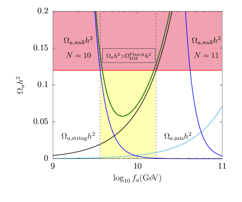
In order to do that, it is convenient, first, to study separately the behavior of the three axion production mechanisms which results are shown in Fig. 1. Specifically, the cyan and black lines show the axion abundances produced by misalignment and global string decay mechanisms, respectively. On the other hand, the blue lines show the abundance of axion dark matter due to the decay of domain wall systems for and , calculated for the coupling constant value . Two shaded regions are also shown: the light red one corresponds to the exclusion region coming from the constraint of the over closure of the Universe Ade et al. (2016), and the yellow region gives the possible interval for the axion decay constant , for which no over abundance of axions from decay of global strings or domain walls is produced. Finally, the dark green line corresponds to the total abundance of axions, , as given by Eq. (30), obtained for the case and . The case for is not shown because for all the considered values of the axion relic density is overabundant.
From Fig. 1 some conclusions are straightforward. First, and grow when grows. Thus, in principle, these are dominant for the greater values of (). However, the misalignment mechanism is always subdominant because has an extra global factor. Indeed, the misalignment mechanism contributes at most by for the total dark matter density. In contrast, is decreasing with and thus it dominates for the smaller values of (). That can be understood realizing that the domain-wall time decay is larger for smaller values, making the domain wall more stable and, in this way, explaining why this mechanism contributes more for the axion relic density when is smaller. The opposite behavior of and allow to set an upper and lower bound on . For , is constrained to be in order to satisfy Ade et al. (2016). Actually, the interval of allowed values is slightly thinner because all of the three axion production mechanisms contribute simultaneously. Also, note that the upper bound above is independent on the value of and on the value of , as can be seen from Eq. (28). In contrast, the lower bound is only valid for the case of . Actually, the case of is completely ruled out and, for this reason, our analysis will be concerned exclusively with the symmetry case.
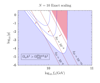
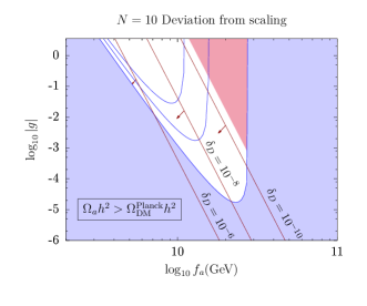
Once we have gained a general knowledge about the behavior of as function of for , we can go further studying the parameter space for the case, allowed by the axion phenomenology. In particular, in Fig. 2 we show the parameter space for the cases of exact scaling (, left frame) and deviation from scaling (, right frame). The range of values of the coupling constant, , has been chosen to include values of . The blue curves correspond to the regions where the total axion dark matter abundance is equal to , taking into account the uncertainties in the parameters and in Eqs. (28) and (29). Notice that for a given value of , is lower bounded by these lines. Larger values of imply . The light blue shaded region is ruled out by the over closure of the Universe for the case of the parameter in Eq. (29) and for the factor in Eq. (28). From the remaining region, it is possible to exclude another large part applying the axion mass stability condition, [see the discussion near Eq. (23)]. Because is directly proportional to and , cf. Eq. (23), and is inversely proportional to , cf. Eq. (24), the forbidden region, denoted by the light red color, is in the top right part of the plane. In addition, in Fig. 2 are shown three dark red lines which correspond to the NEDM constraint, given by Eq. (22), for different values of . It is important to realize that values of order one (not shown) do not give allowed regions in the parameter space. It is necessary to allow in order to have nonexcluded regions which are below the lines. In particular, we calculate the maximum values of that give allowed regions in the parameter space. The corresponding results, in the cases of exact scaling () and deviation from scaling (), are
| (31) |
These values are obtained by taking , and considering the uncertainties in the parameters of the three axion production mechanisms. Lower values of would require higher tuning on the parameter, with values of the order as shown in Fig. 2. In general, for fixed, the tuning on depends on the decay constant and the mechanism of axion dark matter production: if the decay of domain walls was dominant (left side of the curves), the tuning would be less severe than if the production by string decay (right side of the curves) was the dominant one.
Also, in Fig. 2 is shown that for a small enough in order to satisfy the NEDM condition, and for a given value between and , there are two separated regions for where axions can make up the total DM relic density. For instance, taking and considering the uncertainties in the parameters, these regions and their corresponding axion masses for the exact scaling case, are
| (32) |
In the first range for the production of dark matter is mainly through the decay of domain walls, while in the second range it is due to the decay of strings. Taking smaller values for , will lead to more stringent intervals for both and . For the case of deviation from scaling, we find , corresponding to , when the domain walls decay is the leading production mechanism, and , leading to , for the string decay as the dominant contribution.
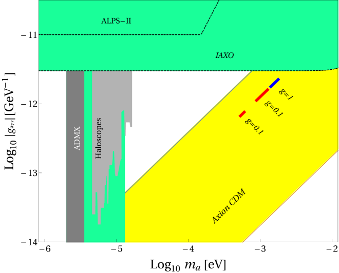
Finally, for values of of order one, we can make predictions regarding the observability of axion in current and/or future experiments. Specifically, the axion coupling to two photons, , depends on the decay constant, the electromagnetic and color anomaly coefficients, and , respectively. It is known that these anomaly coefficients are completely determined by the fermion content and the U charges of the model, cf. Table (2). Standard calculations for anomaly coefficients Srednicki (1985); Carvajal et al. (2015) furnish and . With this information, we can go further plotting, in Fig 3, as a function of for the regions where axions make up the total dark matter relic density and for two different values of , specifically and . This figure clearly shows two allowed regions for : with and with , and one region for : with . The reason why there is only one region for larger values is that the gravitational mass grows with and thus, it conflicts with the condition for lower axion masses. Moreover, it is notable that for the range with larger masses (blue line), the axion parameters of this model are very close to the projected region which is going to be explored by the IAXO experiment Ringwald and Saikawa (2016); Dafni and et al. (2016).
VI Conclusions
In this work, we consider a version of an alternative electroweak model based on the gauge symmetry, the so called models, when the color gauge group is added. For this version, which includes right-handed neutrinos, it is shown in Ref. Montero and Sánchez-Vega (2011) that the PQ mechanism for the solution of the strong problem can be implemented. In this implementation, the axion, the pseudo Nambu-Goldstone boson that emerges from the PQ-symmetry breaking, is made invisible by the introduction of the scalar singlet whose VEV, , is much larger than , and any other VEV in the model. Moreover, the axion is also protected against gravitational effects, that could destabilize its mass, by a discrete symmetry, with .
Once we have set this consistent scenario, we investigate the capabilities of this axion, produced in the framework of this particular model, to be a postinflationary cold dark matter candidate. We started focusing in the axion-production mechanisms. As it was explained in the previous section, from Fig. 1 we see that the vacuum misalignment mechanism does not dominate the DM relic abundance, and, if it was the only production mechanism in action, an upper bound for could be set by imposing that it should account for all the DM abundance, i.e., , and we would find the corresponding value , for the parameters determined by the model, in this case However, there are two other more efficient mechanisms due to the decay of topological defects: cosmic strings and domain walls. As the curves for and grow in opposite directions, relatively to the values, we can determine an upper bound and a lower bound for by imposing the total matches the observed Planck results. This is the case when we add up all the contributions for , and we find . However, we would like to stress that this is not the case for . For there is no value of for which the addition of the partial abundances lies below the observed result. It means that the , which possesses the good quality of stabilizing the axion, is not appropriate for the axion-production issue since it makes the domain wall mechanism too efficient and overpopulates the Universe.
As it can be seen from Fig. 1, for any fixed allowed value of , there are two values of that are in agreement with the value of . In fact they are regions, if we take into account the uncertainties following the discussion in the previous section for Fig. 2. Outside these regions, the axion abundance will be a fraction of . See the solid dark green curve in Fig. 1 for . If this happens to be the case, i.e., if these predicted regions are somehow excluded, by future experimental data for the axion mass value, for instance, then, another kind of DM will be needed. We have also found special values for , , by requiring the minimal compatible intersection region between the curves that obey the NEDM and constraints. This value was obtained considering the maximum value of , i.e., , cf. Fig. 22(a). For lower values of , higher tuning on is required. However, it seems unnatural to require severe levels of tuning on , since for this quantity a tiny value is the result of the difference between two terms that have completely different origins.
Regarding the capabilities of detecting the axion dark matter, Fig. 3 shows the sensitivities of several experiments in the plane. In this plot, the thick blue and red lines are the regions where the axion abundance is responsible for all the observed DM. These lines were obtained by using of order one. Moreover, the blue region corresponding to masses of the order of meV and , lies very close to the projected IAXO sensitivity, so that it will be reachable in the near future.
Looking back to our results we can conclude that this version of the model, concerning the axion DM issue and the strong problem, is phenomenologically consistent. This model, besides its good qualities presented in the introduction, also possesses new degrees of freedom that are not yet experimentally probed. For instance, the model has charged and neutral scalars (besides the Higgs), extra vector bosons and extra quarks, that are expected to be heavy, and could, in principle, be searched at colliders. See Refs. Cao and Zhang ; Corcella et al. (2017) for recent studies concerning the model phenomenology, in general, at the LHC.
Acknowledgements.
B. L. S. V. is thankful for the support of FAPESP funding Grant No. 2014/19164-6. A. R. R. C would like to thank Coordenação de Aperfeiçoamento de Pessoal de Nível Superior (CAPES), Brasil, for financial support.References
- (1) G. Bertone and D. Hooper, arXiv:1605.04909 .
- Bertone et al. (2005) G. Bertone, D. Hooper, and J. Silk, Phys. Rep. 405, 279 (2005).
- Bergström (2012) L. Bergström, Ann. Phys. (Berlin) 524, 479 (2012).
- ATLAS Collaboration (2016) ATLAS Collaboration, J. High Energy Phys. 9, 175 (2016).
- Dias et al. (2014) A. G. Dias, A. C. B. Machado, C. C. Nishi, A. Ringwald, and P. Vaudrevange, J. High Energy Phys. 06, 037 (2014).
- Graham et al. (2015) P. W. Graham, I. G. Irastorza, S. K. Lamoreaux, A. Lindner, and K. A. van Bibber, Annu. Rev. Nucl. Part. Sci. 65, 485 (2015).
- Battaglieri and et al. (2017) M. Battaglieri and et al., (2017), arXiv:1707.04591 .
- Kim and Carosi (2010) J. E. Kim and G. Carosi, Rev. Mod. Phys. 82, 557 (2010).
- Preskill et al. (1983) J. Preskill, M. B. Wise, and F. Wilczek, Phys. Lett. 120B, 127 (1983).
- Abbott and Sikivie (1983) L. Abbott and P. Sikivie, Phys. Lett. 120B, 133 (1983).
- Dine and Fischler (1983) M. Dine and W. Fischler, Phys. Lett. 120B, 137 (1983).
- Carvajal et al. (2017) C. D. R. Carvajal, B. L. Sánchez-Vega, and O. Zapata, Phys. Rev. D 96, 115035 (2017).
- Sánchez-Vega and Schmitz (2015) B. L. Sánchez-Vega and E. R. Schmitz, Phys. Rev. D 92, 053007 (2015).
- Sánchez-Vega et al. (2014) B. L. Sánchez-Vega, J. C. Montero, and E. R. Schmitz, Phys. Rev. D 90, 055022 (2014).
- Pires and Ravinez (1998) C. A. d. S. Pires and O. P. Ravinez, Phys. Rev. D 58, 035008 (1998).
- Pisano and Pleitez (1992) F. Pisano and V. Pleitez, Phys. Rev. D 46, 410 (1992).
- Frampton (1992) P. H. Frampton, Phys. Rev. Lett. 69, 2889 (1992).
- Foot et al. (1993) R. Foot, O. F. Hernández, F. Pisano, and V. Pleitez, Phys. Rev. D 47, 4158 (1993).
- Dias et al. (2005a) A. G. Dias, R. Martinez, and V. Pleitez, Eur. Phys. J. C 39, 101 (2005a).
- Montero and Sánchez-Vega (2011) J. C. Montero and B. L. Sánchez-Vega, Phys. Rev. D 84, 055019 (2011).
- Foot et al. (1994) R. Foot, H. N. Long, and T. A. Tran, Phys. Rev. D 50, R34 (1994).
- Montero et al. (1993) J. C. Montero, F. Pisano, and V. Pleitez, Phys. Rev. D 47, 2918 (1993).
- S. de Pires and Rodrigues da Silva (2004) C. A. S. de Pires and P. S. Rodrigues da Silva, Eur. Phys. J. C 36, 397 (2004).
- Dias et al. (2005b) A. G. Dias, C. A. de S. Pires, and P. S. R. da Silva, Phys. Lett. B 628, 85 (2005b).
- Dong et al. (2006) P. V. Dong, T. T. Huong, D. T. Huong, and H. N. Long, Phys. Rev. D 74, 053003 (2006).
- Dong et al. (2007) P. V. Dong, H. N. Long, and D. V. Soa, Phys. Rev. D 75, 073006 (2007).
- Mizukoshi et al. (2011) J. K. Mizukoshi, C. A. de S. Pires, F. S. Queiroz, and P. S. R. da Silva, Phys. Rev. D 83, 065024 (2011).
- Dias and Pleitez (2004) A. G. Dias and V. Pleitez, Phys. Rev. D 69, 077702 (2004).
- Cogollo et al. (2014) D. Cogollo, A. X. Gonzalez-Morales, F. S. Queiroz, and P. R. Teles, J. Cosmol. Astropart. Phys. 11, 002 (2014).
- Montero and Sánchez-Vega (2015) J. C. Montero and B. L. Sánchez-Vega, Phys. Rev. D 91, 037302 (2015).
- Boucenna et al. (2015) S. M. Boucenna, J. W. F. Valle, and A. Vicente, Phys. Rev. D 92, 053001 (2015).
- Clavelli and Yang (1974) L. Clavelli and T. C. Yang, Phys. Rev. D 10, 658 (1974).
- Lee and Weinberg (1977) B. W. Lee and S. Weinberg, Phys. Rev. Lett. 38, 1237 (1977).
- Lee and Shrock (1978) B. W. Lee and R. E. Shrock, Phys. Rev. D 17, 2410 (1978).
- Singer (1979) M. Singer, Phys. Rev. D 19, 296 (1979).
- Singer et al. (1980) M. Singer, J. W. F. Valle, and J. Schechter, Phys. Rev. D 22, 738 (1980).
- B. L. Sánchez-Vega et al. (2018) B. L. Sánchez-Vega, E. R. Schmitz, and J. C. Montero, Eur. Phys. J. C 78, 166 (2018).
- Kim (1979) J. E. Kim, Phys. Rev. Lett.. 43, 103 (1979).
- Dine et al. (1981) M. Dine, W. Fischler, and M. Srednicki, Phys. Lett. 104B, 199 (1981).
- Georgi and Wise (1982) H. Georgi and M. B. Wise, Phys. Lett. 116B, 123 (1982).
- Srednicki (1985) M. Srednicki, Nucl. Phys. B 260, 689 (1985).
- Bardeen et al. (1987) W. A. Bardeen, R. Peccei, and T. Yanagida, Nucl. Phys. B279, 401 (1987).
- Kamionkowski and March-Russell (1992) M. Kamionkowski and J. March-Russell, Phys. Lett. B 282, 137 (1992).
- Holman et al. (1992) R. Holman, S. D. Hsu, T. W. Kephart, E. W. Kolb, R. Watkins, and L. M. Widrow, Phys. Lett. B 282, 132 (1992).
- Krauss and Wilczek (1989) L. M. Krauss and F. Wilczek, Phys. Rev. Lett. 62, 1221 (1989).
- Ibáñez (1993) L. E. Ibáñez, Nucl. Phys. B398, 301 (1993).
- Babu et al. (2003a) K. S. Babu, I. Gogoladze, and K. Wang, Phys. Lett. B 560, 214 (2003a).
- Babu et al. (2003b) K. Babu, I. Gogoladze, and K. Wang, Nucl. Phys. B660, 322 (2003b).
- Ibáñez and Ross (1991) L. E. Ibáñez and G. G. Ross, Phys. Lett. B 260, 291 (1991).
- Banks and Dine (1992) T. Banks and M. Dine, Phys. Rev. D 45, 1424 (1992).
- Luhn and Ramond (2008) C. Luhn and P. Ramond, JHEP 07, 085 (2008), 0805.1736 .
- Turner and Wilczek (1991) M. S. Turner and F. Wilczek, Phys. Rev. Lett. 66, 5 (1991).
- Harari and Sikivie (1987) D. Harari and P. Sikivie, Phys. Lett. B 195, 361 (1987).
- Vilenkin and Everett (1982) A. Vilenkin and A. E. Everett, Phys. Rev. Lett. 48, 1867 (1982).
- Kawasaki et al. (2015) M. Kawasaki, K. Saikawa, and T. Sekiguchi, Phys. Rev. D 91, 065014 (2015).
- Wantz and Shellard (2010a) O. Wantz and E. P. S. Shellard, Nucl. Phys. B 829, 110 (2010a).
- Wantz and Shellard (2010b) O. Wantz and E. P. S. Shellard, Phys. Rev. D 82, 123508 (2010b).
- Kolb and Turner (1994) E. Kolb and M. Turner, The Early Universe, Vol. 69 (Addison-Wesley, New York, 1994).
- Vilenkin (1985) A. Vilenkin, Phys. Rep. 121, 263 (1985).
- Davis (1986) R. L. Davis, Phys. Lett. B 180, 225 (1986).
- Hiramatsu et al. (2011) T. Hiramatsu, M. Kawasaki, T. Sekiguchi, M. Yamaguchi, and J. Yokoyama, Phys. Rev. D 83, 123531 (2011).
- Hiramatsu et al. (2012) T. Hiramatsu, M. Kawasaki, K. Saikawa, and T. Sekiguchi, Phys. Rev. D 85, 105020 (2012).
- Sikivie (1982) P. Sikivie, Phys. Rev. Lett. 48, 1156 (1982).
- Vilenkin and Shellard (1994) A. Vilenkin and E. P. S. Shellard, Cosmic Strings and Other Topological Defects, Cambridge Monographs on Mathematical Physics (Cambridge University Press, Cambridge, England, 1994).
- Lyth (1992) D. H. Lyth, Phys. Lett. B 275, 279 (1992).
- Ringwald and Saikawa (2016) A. Ringwald and K. Saikawa, Phys. Rev. D 93, 085031 (2016).
- Ade et al. (2016) P. A. R. Ade et al. (Planck), Astron. Astrophys. 594, A13 (2016).
- Carvajal et al. (2015) C. D. R. Carvajal, A. G. Dias, C. C. Nishi, and B. L. Sánchez-Vega, 05, 069 (2015), [Erratum: JHEP08,103(2015)].
- Dafni and et al. (2016) T. Dafni and et al., Nuclear and Particle Physics Proceedings 273, 244 (2016).
- Bastidon (2015) N. Bastidon (ALPS II), in Proceedings, 11th Patras Workshop on Axions, WIMPs and WISPs (Axion-WIMP 2015): Zaragoza, Spain, June 22-26, 2015 (Verlag Deutsches Elektronen-Synchrotron, Hamburg, 2015) p. 31.
- Bähre et al. (2013) R. Bähre, B. Döbrich, J. Dreyling-Eschweiler, S. Ghazaryan, R. Hodajerdi, D. Horns, F. Januschek, E.-A. Knabbe, A. Lindner, D. Notz, et al., J. Instrum. 8, T09001 (2013).
- Armengaud et al. (2014) E. Armengaud, F. Avignone, M. Betz, P. Brax, P. Brun, G. Cantatore, J. Carmona, G. Carosi, F. Caspers, S. Caspi, et al., J. Instrum. 9, T05002 (2014).
- (73) Q.-H. Cao and D.-M. Zhang, arXiv preprint arXiv:1611.09337 .
- Corcella et al. (2017) G. Corcella, C. Corianò, A. Costantini, and P. H. Frampton, Phys. Lett. B 773, 544 (2017).