An adaptive, implicit, conservative 1D-2V multi-species Vlasov-Fokker-Planck multiscale solver in planar geometry

Abstract

We consider a 1D-2V Vlasov-Fokker-Planck multi-species ionic description coupled to fluid electrons. We address temporal stiffness with implicit time stepping, suitably preconditioned. To address temperature disparity in time and space, we extend the conservative adaptive velocity-space discretization scheme proposed in [Taitano et al., J. Comput. Phys., 318, 391–420, (2016)] to a spatially inhomogeneous system. In this approach, we normalize the velocity-space coordinate to a temporally and spatially varying local characteristic speed per species. We explicitly consider the resulting inertial terms in the Vlasov equation, and derive a discrete formulation that conserves mass, momentum, and energy up to a prescribed nonlinear tolerance upon convergence. Our conservation strategy employs nonlinear constraints to enforce these properties discretely for both the Vlasov operator and the Fokker-Planck collision operator. Numerical examples of varying degrees of complexity, including shock-wave propagation, demonstrate the favorable efficiency and accuracy properties of the scheme.

1 Introduction

The Vlasov-Fokker-Planck (VFP) collisional kinetic description, coupled with Maxwell’s equations, is regarded as a first-principles physical model for describing weakly coupled plasmas in all collisionality regimes, and accordingly, has a wide range of applications in laboratory (e.g., magnetic and inertial thermonuclear fusion), space (e.g., Earth’s magnetosphere), and astrophysical (e.g., stellar mass ejections) plasmas. In the VFP system, collisions are modeled by the Fokker-Planck collision operator, which describes collisional relaxation of particle distribution functions in plasmas under the assumption of binary, grazing-angle collisions [1, 2, 3, 4, 5, 6]. Mathematically, the Fokker-Planck operator is integro-differential, non-local, and very difficult to invert.

The system of VFP equations for various plasma species supports disparate length and time scales, as well as arbitrary temperature disparity in time and space, which makes this system particularly challenging to solve with grid-based approaches. The challenges of temperature disparity are evident when one considers the thermal speed, $v_{th}=\sqrt{2T/m}$, which provides a characteristic width of the plasma species distribution function and is a function of the plasma temperature, $T$, and particle species mass, $m$. In many practical applications of interest, $v_{th}$ variation for a given species can span several orders of magnitude in configuration space. In addition, mass differences result in strong $v_{th}$ disparities for different species. Since the velocity-space domain size is determined for a given species by the hottest region (large $v_{th}$), and the velocity-grid spacing must resolve the coldest region (small $v_{th}$), velocity-space discretizations with uniform Cartesian grids in such scenarios may lead to impractical grid size requirements.

Several studies recognized and tried to address these challenges by normalizing the velocity coordinate to the local thermal velocity [7, 8, 9, 10]. In this fashion, the grid will expand as the plasma heats, and contract as it cools. Particularly relevant to this study is the work in Ref. [8], where the velocity-space domain was adapted for multiple ion species based on a single local average $v_{th}$ (over the ion species) and hydrodynamic velocity of the plasma. This powerful strategy enabled the fully kinetic implosion simulations of inertial confinement fusion (ICF) capsules [8, 11, 12], but required intermittent remapping in both the physical and velocity space. None of these strategies conserve mass, momentum, and energy, and some of them [9] break the structured nature of the underlying computational mesh.

Recently, a novel strategy that deals with strong temperature disparity, avoids remapping, and works on structured meshes was proposed in Ref. [13] for the 0D-2V multispecies Fokker-Planck equation. The strategy employs a multiple-grid approach by normalizing each species’ velocity to its thermal speed. The Fokker-Planck equation was transformed analytically, and then discretized on a mesh. The transformed equations exposed the continuum conservation symmetries, which were then enforced in the discrete via nonlinear constraints. This strategy ensures that the species’ distribution function is always well resolved regardless of temperature or mass disparity.

In this study, we extend the conservative, multiple-dynamic velocity-space adaptive strategy developed in Ref. [13] to a spatially inhomogeneous, 1D Cartesian system. We consider a quasi-neutral plasma with multiple kinetic ion species and fluid electrons. As before, ionic species are evolved on a velocity-space grid normalized to a temporally and spatially varying characteristic speed, $v^{*}$ (a function of their $v_{th}$), and the VFP equation is analytically transformed. This transformation introduces additional inertial terms, which are carefully discretized to ensure simultaneous conservation of mass, momentum, and energy.

The rest of the paper is organized as follows. Section 2 introduces the VFP and fluid-electron equations and discusses their conservation properties. In Sec. 3, we introduce the normalized Vlasov equation, and provide a detailed discussion on the implementation of the proposed schemes in the following order: 1) a discretization of the Vlasov-Fokker-Planck equation with the additional inertial terms, 2) a discretization of the fluid electron equation, 3) our discrete conservation strategy for fluid electrons and kinetic ions, 4) a discrete conservation strategy for the Vlasov component with the added inertial terms, and 5) temporal and spatial evolution of $v^{*}$. The numerical performance of the scheme is demonstrated with various multi-species tests of varying degrees of complexity in Sec. 4. Finally, we conclude in Sec. 5.

2 The multi-species Vlasov-Rosenbluth-Fokker-Planck equation with fluid electrons

A dynamic evolution of weakly-coupled collisional plasmas is described by the Vlasov-Fokker-Planck equation for the particle distribution function (PDF), $f\left(\mathbf{\mathbf{x},\mathbf{v},t}\right)$ in configuration space, $\mathbf{x}$, velocity space, $\mathbf{v}$, and time, $t$:

$$\partial_{t}f_{\alpha}+\nabla_{x}\cdot\left(\mathbf{v}f_{\alpha}\right)+\frac{q_{\alpha}}{m_{\alpha}}\nabla_{v}\cdot\left[\left(\mathbf{E}+\mathbf{v}\times\mathbf{B}\right)f_{\alpha}\right]=\sum_{\beta=1}^{N_{s}}C_{\alpha\beta},$$ (2.1)

where $\mathbf{E}$ is the electric field, $\mathbf{B}$ is the magnetic field, $N_{s}$ is the total number of plasma species in the system, and $C_{\alpha\beta}$ is the Fokker-Planck collision operator for species $\alpha$ colliding with species $\beta$:

$$C_{\alpha\beta}=\Gamma_{\alpha\beta}\nabla_{v}\cdot\left[\stackrel{{\scriptstyle\leftrightarrow}}{{\mathsfsl{D}}}_{\beta}\cdot\nabla_{v}f_{\alpha}-\frac{m_{\alpha}}{m_{\beta}}\mathbf{{A}}_{\beta}f_{\alpha}\right].$$ (2.2)

Here, $\Gamma_{\alpha\beta}=\frac{2\pi Z_{\alpha}^{2}Z_{\beta}^{2}e^{4}\Lambda_{\alpha\beta}}{m_{\alpha}^{2}},$ $\stackrel{{\scriptstyle\leftrightarrow}}{{\mathsfsl{D}}}{}_{\beta}$ and $\mathbf{{A}}_{\beta}$ are the tensor-diffusion and friction coefficients for species $\beta$, $m_{\alpha}$ and $m_{\beta}$ are the masses of species $\alpha$ and $\beta$, respectively, $Z_{\alpha}=q_{\alpha}/e$ is the ionization state of species $\alpha$, $e$ is the proton charge, and $\Lambda_{\alpha\beta}$ is the Coulomb logarithm ($\Lambda_{\alpha\beta}=10$ is assumed for simplicity in this study for all species).

The Rosenbluth formulation of the Fokker-Planck collision operator [1] computes the velocity-space-transport coefficients from the so-called Rosenbluth potentials $G_{\beta}$, $H_{\beta}$ as:

$$\stackrel{{\scriptstyle\leftrightarrow}}{{\mathsfsl{D}}}_{\beta} = \nabla_{v}\nabla_{v}G_{\beta},$$ (2.3)

$$\mathbf{A}_{\beta} = \nabla_{v}H_{\beta},$$ (2.4)

which, in turn, are computed from the distribution function of species $\beta$ as:

$$\nabla_{v}^{2}H_{\beta}=-8\pi f_{\beta},$$ (2.5)

$$\nabla_{v}^{2}G_{\beta}=H_{\beta}.$$ (2.6)

The Rosenbluth form is completely equivalent to the integral Landau form [6], but more advantageous algorithmically because it can be inverted with $\mathcal{O}(N)$ complexity (with $N$ the number of degrees of freedom in velocity space) [14].

The collision operator, Eq. (2.2), preserves the positivity of $f_{\alpha}$, and conserves mass, momentum, and energy. The conservation properties stem from the following symmetries [15]:

$$\left<1,C_{\alpha\beta}\right>_{v} = 0,$$ (2.7)

$$m_{\alpha}\left<\mathbf{v},C_{\alpha\beta}\right>_{v} = -m_{\beta}\left<\mathbf{v},C_{\beta\alpha}\right>_{v},$$ (2.8)

$$m_{\alpha}\left<\frac{v^{2}}{2},C_{\alpha\beta}\right>_{v} = -m_{\beta}\left<\frac{v^{2}}{2},C_{\beta\alpha}\right>_{v},$$ (2.9)

where the inner product is defined as $\left<A,B\right>_{v}=2\pi\int_{-\infty}^{\infty}dv_{||}\int_{0}^{\infty}dv_{\perp}v_{\perp}A(\mathbf{v})\,B(\mathbf{v})$ (for the cylindrically symmetric coordinate system in the velocity space employed herein). These conservation symmetries can be enforced in the discrete following the general procedures discussed in Refs. [14, 13].

In this study, we consider a 1D planar geometry in the configuration space without a magnetic field. Without loss of generality, we consider a 2V cylindrically symmetric coordinate system in the velocity space. We adopt a fluid-electron model with a reduced ion-electron collision operator. We obtain the following simplified system of equations comprised of the ion-Vlasov-Fokker-Planck equation (per species $\alpha$),

$$\partial_{t}f_{\alpha}+\partial_{x}\left(v_{||}f_{\alpha}\right)+\frac{q_{\alpha}}{m_{\alpha}}E_{||}\partial_{v_{||}}f_{\alpha}=\sum_{\beta}^{N_{s}}C_{\alpha\beta}+C_{\alpha e}$$ (2.10)

and the electron-temperature equation,

$$\frac{3}{2}\frac{\partial}{\partial t}\left[n_{e}T_{e}\right]+\frac{5}{2}\partial_{x}\left[u_{||,e}n_{e}T_{e}\right]+\partial_{x}Q_{||,e}-q_{e}n_{e}u_{||,e}E_{||}=\sum_{\alpha}^{N_{s}}W_{e\alpha}.$$ (2.11)

Here, $Q_{||,e}$ is the parallel electron-heat flux, $n_{e}$ is the electron density, $T_{e}$ is the electron temperature, $u_{||,e}$ is the parallel electron fluid velocity, $P_{e}=n_{e}T_{e}$ is the electron pressure, $W_{e\alpha}$ describes the electron-ion energy exchange,

$$W_{e\alpha}=F_{||,\alpha e}u_{||,\alpha}+3\nu_{e\alpha}\frac{m_{e}}{m_{\alpha}}n_{e}\left(T_{\alpha}-T_{e}\right),$$ (2.12)

$\mathbf{F}_{\alpha e}^{T}=\left[F_{||,\alpha e},0\right]$ is the friction force between the $\alpha$-ion species and electrons, and

$$\nu_{e\alpha}=\frac{4\sqrt{2\pi}n_{\alpha}q_{\alpha}^{2}e^{4}\Lambda_{e\alpha}}{3\sqrt{m_{e}}T_{e}^{3/2}}$$ (2.13)

is the electron-ion collision frequency. The frictional force between the $\alpha$-ion species and electrons is given by,

$$\mathbf{F}_{\alpha e}=-m_{e}n_{e}\nu_{e\alpha}\left(\mathbf{u}_{\alpha}-\left\langle\mathbf{u}_{\alpha}\right\rangle\right)+\alpha_{0}m_{e}n_{e}\nu_{e\alpha}\left(\mathbf{u}_{e}-\left\langle\mathbf{u}_{\alpha}\right\rangle\right)+\beta_{0}\frac{n_{e}\nu_{e\alpha}\nabla T_{e}}{\sum_{\alpha}^{N_{s}}\nu_{e\alpha}},$$ (2.14)

and the electron heat flux by

$$\mathbf{Q}_{e}=\beta_{0}n_{e}T_{e}\left(\mathbf{u}_{e}-\left\langle\mathbf{u}_{\alpha}\right\rangle\right)-\kappa_{e}\nabla T_{e}.$$ (2.15)

Definitions of coefficients $\alpha_{0},$$\beta_{0}$, $\kappa_{e}$, and the collision-frequency-averaged ion velocity, $\left\langle\mathbf{u}_{\alpha}\right\rangle$, can be found in App. A and in Ref. [16] .

The parallel (to the x-axis) component of the ambipolar-electric field, $E_{||}$, in Eq. (2.11) is found from the inertialess electron momentum equation ,

$$E_{||}=\frac{\sum_{\alpha}^{N_{s}}F_{||,\alpha e}+\partial_{x}P_{e}}{q_{e}n_{e}}.$$ (2.16)

Finally, we assume quasi-neutrality,

$$n_{e}=\sum_{\alpha}^{N_{s}}Z_{\alpha}n_{\alpha},$$ (2.17)

and ambipolarity,

$$u_{||,e}=\frac{\sum_{\alpha}^{N_{s}}Z_{\alpha}nu_{||,\alpha}}{n_{e}},$$ (2.18)

to close the system.

The electron-ion collision operator $C_{\alpha e}$ in Eq. (2.10) is given by:

$$C_{\alpha e}=\Gamma_{\alpha e}\nabla_{v}\cdot\left[\stackrel{{\scriptstyle\leftrightarrow}}{{\mathsfsl{D}}}_{\alpha e}\cdot\nabla_{v}f_{\alpha}-\frac{m_{\alpha}}{m_{e}}\mathbf{A}_{\alpha e}f_{\alpha}\right],$$ (2.19)

where we adopt the reduced ion-electron potentials [17]:

$$G_{\alpha e}=\frac{2}{3}\frac{n_{e}}{\sqrt{\pi}}\frac{\left(\mathbf{v}-\mathbf{u}_{\alpha}\right)\cdot\left(\mathbf{v}-\mathbf{u}_{\alpha}\right)}{v_{th,e}},$$ (2.20)

$$H_{\alpha e}=-\frac{8}{3}\frac{n_{e}}{\sqrt{\pi}v_{th,e}^{3}}\left[\frac{\left(\mathbf{v}-\mathbf{u}_{\alpha}\right)\cdot\left(\mathbf{v}-\mathbf{u}_{\alpha}\right)}{2}-\frac{\mathbf{F}_{\alpha e}}{m_{e}n_{e}\nu_{e\alpha}}\cdot\left(\mathbf{v}-\mathbf{u}_{\alpha}\right)\right].$$ (2.21)

Here, $\mathbf{v}^{T}=\left[v_{||},v_{\perp}\right]$, $\mathbf{u}_{\alpha}^{T}=\left[u_{||,\alpha},0\right]$, $v_{th,e}$ is the electron thermal speed, and the transport coefficients are:

$$\stackrel{{\scriptstyle\leftrightarrow}}{{\mathsfsl{D}}}_{\alpha e}=\nabla_{v}\nabla_{v}G_{\alpha e}=\frac{4}{3}\frac{n_{e}}{\sqrt{\pi}}\frac{\stackrel{{\scriptstyle\leftrightarrow}}{{\mathsfsl{I}}}}{v_{th,e}},$$ (2.22)

$$\mathbf{A}_{\alpha e}=\text{$\mathbf{A}$}_{\alpha e,u}+\mathbf{A}_{\alpha e,F},$$ (2.23)

where $\stackrel{{\scriptstyle\leftrightarrow}}{{\mathsfsl{I}}}$ is the unit dyad,

$$\mathbf{A}_{\alpha e,u}=\nabla_{v}H_{\alpha e,u}=-\frac{8}{3}\frac{n_{e}}{\sqrt{\pi}v_{th,e}^{3}}\left(\mathbf{v}-\mathbf{u}_{\alpha}\right)$$ (2.24)

and

$$\mathbf{A}_{\alpha e,F}=\nabla_{v}H_{\alpha e,F}=\frac{8}{3}\frac{n_{e}}{\sqrt{\pi}v_{th,e}^{3}}\frac{\mathbf{F}_{\alpha e}}{m_{e}n_{e}\nu_{e\alpha}}.$$ (2.25)

2.1 Conservation properties of the kinetic-ion/fluid-electron system

The coupled kinetic-ion and fluid-electron system possesses continuum conservation properties. We remark that, although these properties are well known and have been discussed by others in the past [18], we reproduce them here to explicitly expose the continuum symmetries that are required to ensure the conservation properties. The goal is to develop a strategy that can ensure these properties discretely (Sec. 3.4).

Mass conservation follows trivially from the ion mass conservation and quasi-neutrality. Momentum conservation follows from taking the $m_{\alpha}v_{||}$ moment of the ion Vlasov equation summed over all ions:

$$\sum_{\alpha}^{N_{s}}\left[m_{\alpha}\partial_{t}I_{||,\alpha}+m_{\alpha}\partial_{x}S_{2,||,\alpha}-q_{\alpha}n_{\alpha}E_{||}\right]=\sum_{\alpha}^{N_{s}}m_{\alpha}\left[\sum_{\beta}^{N_{s}}\left\langle v_{||},C\left(f_{\alpha},f_{\beta}\right)\right\rangle_{\mathbf{v}}+\left\langle v_{||},C_{\alpha e}\right\rangle_{\mathbf{v}}\right],$$ (2.26)

where $I_{||,\alpha}=\left\langle v_{||},f_{\alpha}\right\rangle_{\mathbf{v}}$ is the parallel specific momentum density flux, $S_{2,||,\alpha}=\left\langle v_{||},v_{||}f_{\alpha}\right\rangle_{\mathbf{v}}$ is the parallel-parallel component of the pressure tensor, and $q_{\alpha}n_{\alpha}E_{||}=-q_{\alpha}E_{||}\left\langle v_{||},\partial_{v_{||}}f_{\alpha}\right\rangle_{v}$ is the parallel electrostatic force. The first term on the right-hand side (RHS) of Eq. (2.26) vanishes due to momentum conservation across ion species [14]. The second term on the RHS uses the reduced-collision operator between ion species and electrons, and it can be expanded as follows:

$$m_{\alpha}\left\langle v_{||},C_{\alpha e}\right\rangle_{\mathbf{v}}=m_{\alpha}\Gamma_{\alpha e}\left\langle v_{||},\nabla_{v}\cdot\left[\stackrel{{\scriptstyle\leftrightarrow}}{{\mathsfsl{D}}}_{\alpha e}\cdot\nabla f_{\alpha}-\frac{m_{\alpha}}{m_{e}}\mathbf{A}_{\alpha e}f_{\alpha}\right]\right\rangle_{\mathbf{v}}$$

$$=m_{\alpha}\Gamma_{\alpha e}\left[\underbrace{\left\langle v_{||},\nabla_{v}\cdot\left[\stackrel{{\scriptstyle\leftrightarrow}}{{\mathsfsl{D}}}_{\alpha e}\cdot\nabla_{v}f_{\alpha}\right]\right\rangle_{\mathbf{v}}}_{ⓐ}-\frac{m_{\alpha}}{m_{e}}\left\langle v_{||},\nabla_{v}\cdot\left[\left(\underbrace{\mathbf{A}_{\alpha e,u}}_{ⓑ}+\underbrace{\mathbf{A}_{\alpha e,F}}_{ⓒ}\right)f_{\alpha}\right]\right\rangle_{\mathbf{v}}\right].$$ (2.27)

Here, the terms $ⓐ$ and $ⓑ$ vanish independently:

$$m_{\alpha}\left\langle v_{||},\Gamma_{\alpha e}\nabla_{v}\cdot\left[\stackrel{{\scriptstyle\leftrightarrow}}{{\mathsfsl{D}}}_{\alpha e}\cdot\nabla_{v}f_{\alpha}\right]\right\rangle_{v}=m_{\alpha}\Gamma_{\alpha e}\frac{4}{3}\frac{n_{e}}{v_{th,e}\sqrt{\pi}}\left\langle v_{||},\nabla_{v}\cdot\left[\stackrel{{\scriptstyle\leftrightarrow}}{{\mathsfsl{I}}}\cdot\nabla_{v}f_{\alpha}\right]\right\rangle_{v}=0$$ (2.28)

and

$$m_{\alpha}\Gamma_{\alpha e}\left\langle v_{||},\nabla_{v}\cdot\left[\frac{m_{\alpha}}{m_{e}}\mathbf{A}_{\alpha e,u}f_{\alpha}\right]\right\rangle_{v}=-m_{\alpha}\Gamma_{\alpha e}\frac{m_{\alpha}}{m_{e}}\frac{8}{3}\frac{n_{e}}{v_{th,e}^{3}\sqrt{\pi}}\left\langle v_{||},\nabla_{v}\cdot\left[\left(\mathbf{v}-\mathbf{u}_{\alpha}\right)f_{\alpha}\right]\right\rangle_{v}=0.$$ (2.29)

The term $ⓒ$ becomes [by Eq. (2.25)]:

$$m_{\alpha}\Gamma_{\alpha e}\left\langle v_{||},\nabla_{v}\cdot\left[\frac{m_{\alpha}}{m_{e}}\mathbf{A}_{\alpha e,F}f_{\alpha}\right]\right\rangle_{\mathbf{v}}=-F_{||,\alpha e}.$$ (2.30)

When combined with quasi-neutrality, Eq. (2.17), and the ion electrostatic acceleration term:

$$\sum_{\alpha}^{N_{s}}q_{\alpha}n_{\alpha}E_{||}=-\left(\partial_{x}P_{e}+\sum_{\alpha}^{N_{s}}F_{||,\alpha e}\right),$$ (2.31)

Eq. 2.26 yields the total plasma momentum equation

$$\sum_{\alpha}^{N_{s}}m_{\alpha}\left[\partial_{t}I_{\alpha}+\partial_{x}S_{2,||,\alpha}\right]+\partial_{x}P_{e}=0,$$ (2.32)

which is in a conservative form.

To show energy conservation, we take the second moment ($m_{\alpha}\frac{v^{2}}{2}$) of the ion Vlasov equation as:

$$\sum_{\alpha}^{N_{s}}\left[m_{\alpha}\partial_{t}U_{\alpha}+m_{\alpha}\partial_{x}S_{3,||,\alpha}-q_{\alpha}n_{\alpha}u_{||,\alpha}E_{||}\right]=\sum_{\alpha}^{N_{s}}m_{\alpha}\left[\sum_{\beta}^{N_{s}}\left\langle\frac{v^{2}}{2},C\left(f_{\alpha},f_{\beta}\right)\right\rangle_{\mathbf{v}}+\left\langle\frac{v^{2}}{2},C_{\alpha e}\right\rangle_{\mathbf{v}}\right].$$ (2.33)

Here, $U_{\alpha}=\left\langle\frac{v^{2}}{2},f_{\alpha}\right\rangle_{\mathbf{v}}$ is the specific-energy density, $S_{3,\alpha,||}=\left\langle v_{||}\frac{v^{2}}{2},f_{\alpha}\right\rangle_{\mathbf{v}}$ is the parallel component of the specific-energy density flux, and $q_{\alpha}n_{\alpha}u_{||,\alpha}E_{||}=-q_{\alpha}E_{||}\left\langle\frac{v^{2}}{2},\partial_{v_{||}}f_{\alpha}\right\rangle$. The first term on the RHS vanishes owing to energy conservation across ion species. The second term on the RHS can be expanded as follows:

$$m_{\alpha}\left\langle\frac{v^{2}}{2},C_{\alpha e}\right\rangle_{\mathbf{v}}=m_{\alpha}\Gamma_{\alpha e}\left[\underbrace{\left\langle\frac{v^{2}}{2},\nabla_{v}\cdot\left[\stackrel{{\scriptstyle\leftrightarrow}}{{\mathsfsl{D}}}_{\alpha e}\cdot\nabla f_{\alpha}\right]\right\rangle_{\mathbf{v}}}_{ⓐ}-\frac{m_{\alpha}}{m_{e}}\left\langle\frac{v^{2}}{2},\nabla_{v}\cdot\left[\left(\underbrace{\mathbf{A}_{\alpha e,u}}_{ⓑ}+\underbrace{\mathbf{A}_{\alpha e,F}}_{ⓒ}\right)f_{\alpha}\right]\right\rangle_{\mathbf{v}}\right].$$ (2.34)

Here, terms $ⓐ$, $ⓑ$, and $ⓒ$ independently yield [using Eq. (2.22) and (2.23)]:

$$\Gamma_{\alpha e}m_{\alpha}\left\langle\frac{v^{2}}{2},\nabla_{v}\cdot\left[\stackrel{{\scriptstyle\leftrightarrow}}{{\mathsfsl{D}}}_{\alpha e}\cdot\nabla_{v}f_{\alpha}\right]\right\rangle_{v}=m_{\alpha}\Gamma_{\alpha e}\frac{4}{3}\frac{n_{e}}{v_{th,e}\sqrt{\pi}}\left\langle\frac{v^{2}}{2},\nabla_{v}\cdot\left[\stackrel{{\scriptstyle\leftrightarrow}}{{\mathsfsl{I}}}\cdot\nabla_{v}f_{\alpha}\right]\right\rangle_{v}=3\nu_{e\alpha}\frac{m_{e}}{m_{\alpha}}n_{e}T_{e},$$ (2.35)

$$m_{\alpha}\Gamma_{\alpha e}\left\langle\frac{v^{2}}{2},\nabla_{v}\cdot\left[\frac{m_{\alpha}}{m_{e}}\mathbf{A}_{\alpha e,u}f_{\alpha}\right]\right\rangle_{v}=3\nu_{e\alpha}\frac{m_{e}}{m_{\alpha}}n_{e}T_{\alpha},$$ (2.36)

and

$$m_{\alpha}\Gamma_{\alpha e}\left\langle\frac{v^{2}}{2},\nabla_{v}\cdot\left[\frac{m_{\alpha}}{m_{e}}\mathbf{A}_{\alpha e,F}f_{\alpha}\right]\right\rangle_{v}=-u_{||,\alpha}F_{||,\alpha e}.$$ (2.37)

Gathering terms, the energy moment of the ion-electron collision operator yields:

$$m_{\alpha}\left\langle\frac{v^{2}}{2},C_{\alpha e}\right\rangle_{v}=3\nu_{e\alpha}\frac{m_{e}}{m_{\alpha}}n_{e}\left(T_{e}-T_{\alpha}\right)+u_{||,\alpha}F_{||,\alpha e}=-W_{e\alpha}.$$ (2.38)

Using the fluid electron temperature equation and ambipolarity, we finally obtain:

$$\partial_{t}\left(\frac{3}{2}n_{e}T_{e}+\sum_{\alpha}^{N_{s}}m_{\alpha}U_{\alpha}\right)+\partial_{x}\left(\frac{5}{2}u_{||,e}n_{e}T_{e}+\sum_{\alpha}^{N_{s}}m_{\alpha}S_{3,\alpha,||}+Q_{||,e}\right)=0,$$ (2.39)

which is a conservative form of the evolution equation for the total plasma energy density $\frac{3}{2}n_{e}T_{e}+\sum_{\alpha}^{N_{s}}m_{\alpha}U_{\alpha}$.

3 Numerical implementation

3.1 VFP equation in normalized velocity variables

We consider the normalization of all velocity-space quantities for a species $\alpha$ to a reference speed, $v_{\alpha}^{*}\left(x,t\right)$, related to their thermal speed, as follows:

$$\mathbf{\widehat{v}}_{\alpha}=\frac{\mathbf{v}}{v_{\alpha}^{*}},\;\partial_{\widehat{v}_{||}}=v_{\alpha}^{*}\partial_{\widehat{v}_{||}},\;\widehat{f}_{\alpha}=\left(v_{\alpha}^{*}\right)^{3}f_{\alpha}.$$

Here, the hat denotes quantities normalized to $v_{\alpha}^{*}$. As an example, the density, drift, and temperature moments are defined as:

$$n_{\alpha}=\left\langle 1,\widehat{f}_{\alpha}\right\rangle_{\widehat{v}},\;u_{||,\alpha}=v_{\alpha}^{*}\widehat{u}_{||,\alpha}=v_{\alpha}^{*}\left\langle\widehat{v}_{||},\widehat{f}_{\alpha}\right\rangle_{\widehat{v}},\;T_{\alpha}=\left(v_{\alpha}^{*}\right)^{2}\widehat{T}_{\alpha}=\frac{m_{\alpha}\left(v_{\alpha}^{*}\right)^{2}\left\langle\left(\widehat{\mathbf{v}}-\widehat{\mathbf{u}}_{\alpha}\right)^{2},\widehat{f}_{\alpha}\right\rangle_{\widehat{v}}}{3\left\langle 1,\widehat{f}_{\alpha}\right\rangle_{\widehat{v}}}$$

where $\left\langle\left(\cdot\right),\widehat{f}_{\alpha}\right\rangle_{\widehat{v}}=2\pi\int_{-\infty}^{\infty}d\widehat{v}_{||}\int_{0}^{\infty}\left(\cdot\right)\widehat{f}_{\alpha}\widehat{v}_{\perp}d\widehat{v}_{\perp}$.The normalization of other relevant quantities and the collision operator are discussed in Ref. [13]. We note that, as $v^{*}$ is a function of local $v_{th}$ for a given plasma species (elaborated in Sec. 3.6), the grid will expand as the plasma heats, and contract as it cools; refer to Fig. 3.1.

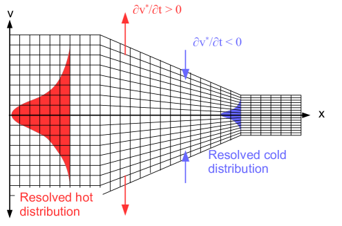
Figure 3.1: Illustration of the velocity space adaptivity.

The temporal and spatial dependence of $v_{\alpha}^{*}$ introduces inertial terms in the Vlasov equation, Eq. (2.10), which after the transformation reads (App. B):

$$\partial_{t}\widehat{f}_{\alpha}+\partial_{x}\left(v_{\alpha}^{*}\widehat{v}_{||}\widehat{f}_{\alpha}\right) + \partial_{\widehat{v}_{||}}\left[\left(\frac{q_{\alpha}}{m_{\alpha}}\frac{E_{||}}{v_{\alpha}^{*}}\right)\widehat{f}_{\alpha}\right]-\widehat{\nabla}_{\widehat{v}}\cdot\left[\left(\frac{\partial_{t}v_{\alpha}^{*}}{v_{\alpha}^{*}}\right)\mathbf{\widehat{v}}\widehat{f}_{\alpha}\right]-\widehat{\nabla}_{\widehat{v}}\cdot\left[\left(\partial_{x}v_{\alpha}^{*}\right)\mathbf{\widehat{v}}\widehat{v}_{||}\widehat{f}_{\alpha}\right]$$ (3.1)

$$= \left(v_{\alpha}^{*}\right)^{3}\left(\sum_{\beta}^{N_{s}}C_{\alpha\beta}+C_{\alpha e}\right)=\sum_{\beta}^{N_{s}}\widehat{C}_{\alpha\beta}+\widehat{C}_{\alpha e}.$$

3.2 Discretization of the VFP equation with inertial terms

We discretize the VFP equation using finite volumes in a 1D planar configuration space ($x$) and 2V cylindrical-velocity space ($\widehat{v}_{||}$ and $\widehat{v}_{\perp}$) with azimuthal symmetry. We compute the discrete volume for cell (i,j,k) as:

$$\Delta V_{i,j,k}=2\pi\Delta x\Delta\widehat{v}_{||}\widehat{v}_{\perp,k}\Delta\widehat{v}_{\perp},$$

where $\Delta x$, $\Delta\widehat{v}_{||}$, and $\Delta\widehat{v}_{\perp}$ are mesh spacings in the configuration space and the parallel- and perpendicular-velocity space, respectively. For a uniform mesh (assumed henceforth), we have:

$$\Delta x=\frac{L_{x}}{N_{x}},\,\,\Delta\widehat{v}_{||}=\frac{L_{||}}{N_{||}},\,\,\Delta\widehat{v}_{\perp}=\frac{L_{\perp}}{N_{\perp}},$$

where $L_{x}$, $L_{||}$, and $L_{\perp}$ are the configuration space, and parallel and perpendicular velocity-space domain sizes, respectively, and $N_{x}$, $N_{||}$, and $N_{\perp}$ are the corresponding number of cells. The mesh is arranged such that cell faces map to the domain boundary (and therefore outermost cell centers are half a mesh-spacing away from the boundary). We define the distribution function $f$ and the Rosenbluth potentials $H$, $G$ at cell centers.

Velocity-space inner products are approximated via a mid-point quadrature rule as

$$\left<A,B\right>_{\widehat{v}}\approx 2\pi\sum_{j=1}^{N_{||}}\sum_{k=1}^{N_{\perp}}\widehat{v}_{\perp,k}\Delta\widehat{v}_{||}\Delta\widehat{v}_{\perp}A_{j,k}B{}_{j,k}$$ (3.2)

for scalars and

$$\left<\mathbf{A},\mathbf{B}\right>_{\widehat{v}}\approx 2\pi\left[\sum_{j=0}^{N_{||}}\sum_{k=1}^{N_{\perp}}\widehat{v}_{\perp,k}\Delta\widehat{v}_{||}\Delta\widehat{v}_{\perp}A_{||,j+1/2,k}B{}_{||,j+1/2,k}+\sum_{j=1}^{N_{||}}\sum_{k=0}^{N_{\perp}}\widehat{v}_{\perp,k+1/2}\Delta\widehat{v}_{||}\Delta\widehat{v}_{\perp}A_{\perp,j,k+1/2}B{}_{\perp,j,k+1/2}\right]$$

for vectors (with components defined at cell faces as denoted by the half-integer indices $j+1/2$, $k+1/2$).

We discretize Eq. (3.1) in a conservative form as

$$\frac{c^{p+1}\widehat{f}_{\alpha,i,j,k}^{p+1}+c^{p}\widehat{f}_{\alpha,i,j,k}^{p}+c^{p-1}\widehat{f}_{\alpha,i,j,k}^{p-1}}{\Delta t}+\underbrace{\frac{F_{\alpha,i+1/2,j,k}^{p+1}-F_{\alpha,i-1/2,j,k}^{p+1}}{\Delta x}}_{ⓐ}+\underbrace{\frac{J_{\alpha,acc,i,j+1/2,k}^{p+1}-J_{\alpha,acc,i,j-1/2,k}^{p+1}}{\Delta\widehat{v}_{||}}}_{ⓑ}$$

$$+\underbrace{\left[\frac{J_{||,\alpha,t,i,j+1/2,k}^{p+1}-J_{||,\alpha,t,i,j-1/2,k}^{p+1}}{\Delta\widehat{v}_{||}}+\frac{\widehat{v}_{\perp,k+1/2}J_{\perp,\alpha,t,i,j,k+1/2}^{p+1}-\widehat{v}_{\perp,k-1/2}J_{\perp,\alpha,t,i,j,k-1/2}^{p+1}}{\widehat{v}_{\perp,k}\Delta\widehat{v}_{\perp}}\right]}_{ⓒ}$$

$$+\underbrace{\left[\frac{J_{||,\alpha,x,i,j+1/2,k}^{p+1}-J_{||,\alpha,x,i,j-1/2,k}^{p+1}}{\Delta\widehat{v}_{||}}+\frac{\widehat{v}_{\perp,k+1/2}J_{\perp,\alpha,x,i,j,k+1/2}^{p+1}-\widehat{v}_{\perp,k-1/2}J_{\perp,\alpha,x,i,j,k-1/2}^{p+1}}{\widehat{v}_{\perp,k}\Delta\widehat{v}_{\perp}}\right]}_{ⓓ}$$

$$=\sum_{\beta}^{N_{s}}\left.C_{\alpha\beta}^{p+1}\right|_{i,j,k}+\left.C_{\alpha e}^{p+1}\right|_{i,j,k}.$$ (3.3)

Here, $c^{p+1}$, $c^{p}$, and $c^{p-1}$ are the coefficients for the second-order backwards difference formula (BDF2) [14] and $p$ is the discrete time index.

The term $ⓐ$ corresponds to the discretization of the spatial streaming term, with

$$F_{\alpha,i+1/2,j,k}^{p+1}=v_{\alpha,i+1/2}^{*,p}\widehat{v}_{||,j}\textnormal{Interp}\left(\widehat{v}_{||,j},\widehat{f}_{\alpha}^{p+1}\right)_{i+1/2,j,k},$$

$$v_{\alpha,i+1/2}^{*}=\frac{v_{\alpha,i+1}^{*}+v_{\alpha,i}^{*}}{2},$$

where $\textnormal{Interp}\left(a,\phi\right)_{face}$ is an advection interpolation operator of a scalar $\phi$ at a cell face based on a given velocity $a$, which can be written in general as

$$\textnormal{Interp}\left(a,\phi\right)_{face}=\sum_{i^{\prime}=1}^{N}\omega_{face,i^{\prime}}\left(a,\phi\right)\phi_{i^{\prime}}.$$ (3.4)

The coefficients $\omega_{face,i^{\prime}}$ are the interpolation weights for the spatial cells $i^{\prime}$ surrounding the cell face of interest (in this study, they are determined by the SMART discretization [19]).

The term $ⓑ$ corresponds to the electrostatic-acceleration term with

$$J_{\alpha,acc,i,j+1/2,k}^{p+1}={\cal A}_{\alpha,i}^{p+1}\textnormal{Interp}\left({\cal A}_{\alpha,i}^{p+1},\widehat{f}_{\alpha}^{p+1}\right)_{i,j+1/2,k},$$ (3.5)

where

$${\cal A}_{\alpha,i}^{p+1}=\frac{q_{\alpha}}{m_{\alpha}}\frac{E_{||,i}^{p+1}}{v_{\alpha,i}^{*,p}}.$$

The term $ⓒ$ corresponds to the inertial term due to temporal variation of the normalization velocity, $v_{\alpha}^{*},$ with

$$J_{||,\alpha,t,i,j+1/2,k}^{p+1}={\cal I}_{\alpha,t,i}^{p}\widehat{v}_{||,j+1/2}\textnormal{Interp}\left({\cal I}_{\alpha,t,i}^{p}\widehat{v}_{||,j+1/2},\widehat{f}_{\alpha}^{p+1}\right)_{i,j+1/2,k}$$

and

$$J_{\perp,\alpha,t,i,j,k+1/2}^{p+1}={\cal I}_{\alpha,t,i}^{p}\widehat{v}_{\perp,k+1/2}\textnormal{Interp}\left({\cal I}_{\alpha,t,i}^{p}\widehat{v}_{\perp,k+1/2},\widehat{f}_{\alpha}^{p+1}\right)_{i,j,k+1/2},$$

where

$${\cal I}_{\alpha,t,i}^{p}=-\frac{\left(\partial_{t}v_{\alpha}^{*,p}\right)_{i}}{v_{\alpha,i}^{*,p}}\approx-\frac{c^{p+1}v_{\alpha,i}^{*,p}+c^{p}v_{\alpha,i}^{*,p-1}+c^{p-1}v_{\alpha,i}^{*,p-2}}{v_{\alpha,i}^{*,p}\Delta t}.$$ (3.6)

We lag the time level between the BDF2 coefficients and the normalization velocity for well-posedness of the velocity-space grid motion [13].

The term $ⓓ$ corresponds to the inertial term due to the spatial variation of the normalization velocity, $v_{\alpha}^{*}$, with

$$J_{||,\alpha,x,i,j+1/2,k}^{p+1}={\cal I}_{\alpha,x,i}^{p}\widehat{v}_{||,j+1/2}^{2}\textnormal{Interp}\left({\cal I}_{\alpha,x,i}^{p},\widehat{f}_{\alpha}^{p+1}\right)_{i,j+1/2,k},$$ (3.7)

$$J_{\perp,\alpha,x,i,j,k+1/2}^{p+1}={\cal I}_{\alpha,x,i}^{p}\widehat{v}_{||,j}\widehat{v}_{\perp,k+1/2}\textnormal{Interp}\left({\cal I}_{\alpha,x,i}^{p}\widehat{v}_{||,j},\widehat{f}_{\alpha}^{p+1}\right)_{i,j,k+1/2},$$ (3.8)

where

$${\cal I}_{\alpha,x,i}^{p}=-\left(\partial_{x}v_{\alpha}^{*,p}\right)_{i}\approx-\frac{v_{\alpha,i+1/2}^{*,p}-v_{\alpha,i-1/2}^{*,p}}{\Delta x}.$$ (3.9)

Finally, the right-hand-side of Eq. (3.3) corresponds to the Fokker-Planck-collision operator and its treatment is discussed in detail in Refs. [14, 13]. In this study, we use the mimetic differencing approach for the tensor diffusion operator in the collision term proposed in Ref. [20].

3.3 Discretization of the electron temperature equation

The electron temperature equation, Eq. (2.11), is also discretized using a finite-volume scheme in space and BDF2 in time:

$$\frac{3}{2}\frac{c^{p+1}n_{e,i}^{p+1}T_{e,i}^{p+1}+c^{p}n_{e,i}^{p}T_{e,i}^{p}+c^{p-1}n_{e,i}^{p-1}T_{e,i}^{p-1}}{\Delta t^{k}}+\frac{5}{2}\frac{u_{||,e,i+1/2}^{p+1}\left(\widetilde{n_{e}T_{e}}\right)_{i+1/2}^{p+1}-u_{||,e,i-1/2}^{p+1}\left(\widetilde{n_{e}T_{e}}\right)_{i-1/2}^{p+1}}{\Delta x}+$$

$$\frac{Q_{||,e,i+1/2}^{p+1}-Q_{||,e,i-1/2}^{p+1}}{\Delta x}-q_{e}\left[\left(n_{e}u_{||,e}\right)_{i}^{E}E_{||,i}\right]^{p+1}=3\nu_{e\alpha,i}^{p+1}\frac{m_{e}}{m_{\alpha}}n_{e,i}^{p+1}\left(T_{\alpha,i}^{p+1}-T_{e,i}^{p+1}\right)+F_{||,\alpha e,i}^{p+1}u_{||,\alpha,i}^{p+1}.$$ (3.10)

Here the tilde denotes a cell-face discretization for the advection quantities (SMART in this study). The quantity with a superscript $E$ in Eq. (3.10) are defined so as to enforce conservation properties, and will be discussed shortly. Other terms in Eq. (3.10) are defined as:

$$u_{||,e,i+1/2}^{p+1}=0.5\left(u_{||,e,i+1}^{p+1}+u_{||,e,i}^{p+1}\right),$$

$$Q_{||,e,i+1/2}^{p+1}=\left[\beta_{0}n_{e}\left(u_{||,e}-\left\langle u_{||,\alpha}\right\rangle\right)\right]_{i+1/2}^{p+1}\widetilde{T}_{e,i+1/2}^{p+1}-\kappa_{||,e,i+1/2}^{p+1}\frac{T_{e,i+1}^{p+1}-T_{e,i}^{p+1}}{\Delta x},$$ (3.11)

where

$$\left[\beta_{0}n_{e}\left(u_{||,e}-\left\langle u_{||,\alpha}\right\rangle\right)\right]_{i+1/2}^{p+1}=0.5\left\{\left[\beta_{0}n_{e}\left(u_{||,e}-\left\langle u_{||,\alpha}\right\rangle\right)\right]_{i+1}^{p+1}+\left[\beta_{0}n_{e}\left(u_{||,e}-\left\langle u_{||,\alpha}\right\rangle\right)\right]_{i}^{p+1}\right\},$$ (3.12)

$$\kappa_{||,e,i+1/2}^{p+1}=0.5\left[\kappa_{||,e,i+1}^{p+1}+\kappa_{||,e,i}^{p+1}\right],$$ (3.13)

$$F_{||,\alpha e,i}^{p+1} = -m_{e}n_{e,i}^{p+1}\nu_{e\alpha,i}^{p+1}\left(u_{||,\alpha,i}^{p+1}-\left\langle u_{||,\alpha,i}\right\rangle^{p+1}\right)+\alpha_{0,i}^{p+1}m_{e}n_{e,i}^{p+1}\nu_{e\alpha,i}^{p+1}\left(u_{||,e,i}^{p+1}-\left\langle u_{||,\alpha,i}\right\rangle^{p+1}\right)$$ (3.14)

$$+\beta_{0,i}^{p+1}\frac{n_{e,i}^{p+1}\nu_{e\alpha,i}^{p+1}}{\sum_{\alpha}^{N_{s}}\nu_{e\alpha,i}^{p+1}}\frac{T_{e,i+1}^{p+1}-T_{e,i-1}^{p+1}}{2\Delta x}.$$

3.4 Definitions for electron quantities to ensure simultaneous discrete conservation of mass, momentum, and energy in the kinetic-ion/fluid-electron system

In this section, we will obtain discrete expressions for the electron density, the electron drift velocity, and the electric field that ensure conservation of mass, momentum, and energy within the kinetic-ion/fluid-electron system.

In Sec. 2.1, we proved that the kinetic-ion-fluid-electron system possesses continuum conservation properties for mass, momentum, and energy. Here, we take an approach similar to that discussed in Refs. [14] and [13], and introduce discrete nonlinear constraints to enforce these properties in the ion-electron collision operator, the electric field, and the Joule-heating term (in the electron temperature equation). The ion-electron collision operator is modified to become

$$\widehat{C}_{\alpha e}=\Gamma_{\alpha e}\widehat{\nabla}_{\widehat{v}}\cdot\left[\gamma_{G,\alpha e}\mathbf{J}_{G,\alpha e}-\frac{m_{\alpha}}{m_{e}}\left[\gamma_{H,\alpha e,u}\mathbf{J}_{H,\alpha e,u}+\gamma_{H,\alpha e,F}\mathbf{J}_{H,\alpha e,F}\right]\right].$$ (3.15)

Here,

$$\mathbf{J}_{G,\alpha e}=\stackrel{{\scriptstyle\leftrightarrow}}{{\mathsfsl{D}}}_{\alpha e}\cdot\nabla_{v}f_{\alpha},$$ (3.16)

$$\mathbf{J}_{H,\alpha e,u}=\mathbf{A}_{\alpha e,u}f_{\alpha},$$ (3.17)

and

$$\mathbf{J}_{H,\alpha e,F}=\mathbf{A}_{\alpha e,F}f_{\alpha}$$ (3.18)

are the collisional-velocity-space fluxes and $\gamma_{G,\alpha e}$, $\gamma_{H,\alpha e,u}$, and $\gamma_{H,\alpha e,F}$ are the nonlinear-constraint functions that ensure discrete conservation of momentum and energy for collisions between kinetic ions and fluid electrons (App. C).

In order to ensure discrete global momentum conservation between kinetic ions and fluid electrons, we require the following relationship in the continuum (Sec. 2.1):

$$\sum_{\alpha}\left[q_{\alpha}E_{||}\left\langle v_{||},\partial_{v_{||}}f\right\rangle_{v}-m_{\alpha}\left\langle v_{||},C_{\alpha e}\right\rangle_{v}\right]=\partial_{x}P_{e}.$$

We specialize this expression at cell centers $i$ as:

$$\sum_{\alpha}\left[q_{\alpha}E_{||}\left\langle v_{||},\partial_{v_{||}}f\right\rangle_{v}-m_{\alpha}\left\langle v_{||},C_{\alpha e}\right\rangle_{v}\right]_{i}=\left.\partial_{x}P_{e}\right|_{i}.$$

The first term in the left-hand side gives:

$$\left\langle v_{||},\partial_{v_{||}}f\right\rangle_{v,i}=-n_{\alpha,i}^{E},$$

where $n_{\alpha,i}^{E}$ is a density computed by integration by parts, but which accounts for the sign of the electric field in the original advection operator as:

$$n_{\alpha,i}^{E}=\sum_{j,k}\Delta\widetilde{V}_{j+1/2,k}\textnormal{Interp}\left(E_{\parallel,i}^{p+1},\widehat{f}_{\alpha}^{p+1}\right)_{i,j+1/2,k}.$$ (3.19)

Here, $\sum_{j,k}\equiv\sum_{j}\sum_{k}$, and $\Delta\widetilde{V}_{j+1/2,k}=2\pi v_{\perp,k}\Delta v_{\perp}\Delta v_{||}$. We define a corresponding electron density by quasineutrality as:

$$n_{e,i}^{E}=\sum_{\alpha}^{N_{s}}Z_{\alpha}n_{\alpha,i}^{E}.$$ (3.20)

The second term in the left-hand side gives:

$$\sum_{\alpha}\left[m_{\alpha}\left\langle v_{||},C_{\alpha e}\right\rangle_{v}\right]_{i}=\left.\sum_{\alpha}F_{\alpha e,||}\right|_{i}$$

when the associated ion-electron collision operator symmetries are satisfied (App. C). There results the following definition of the discrete electric field at spatial cell index $i$:

$$E_{||,i}=\frac{\left(\partial_{x}P_{e}+\sum_{\alpha}F_{\alpha e}\right)_{i}}{q_{e}n_{e,i}^{E}}$$ (3.21)

This result ensures momentum conservation for the kinetic-ion/fluid-electron system.

To ensure energy conservation for the kinetic-ion/fluid-electron system, we require the following relationship in the continuum (which we specialize at the cell $i$):

$$(n_{e}u_{e,||})_{i}^{E}=-\sum_{\alpha}\left[Z_{\alpha}\left\langle\frac{v^{2}}{2},\partial_{v_{||}}f\right\rangle_{v,i}\right].$$ (3.22)

We achieve this discretely as before by computing an electric-field-aware momentum moment as:

$$-\left\langle\frac{v^{2}}{2},\left(\partial_{v_{||}}f\right)\right\rangle_{v,i}=\sum_{j,k}\Delta\widetilde{V}_{j+1/2,k}v_{||,j+1/2}\textnormal{Interp}\left(E_{\parallel,i}^{p+1},\widehat{f}_{\alpha}^{p+1}\right)_{i,j+1/2,k},$$ (3.23)

and compute the fluid-electron Joule-heating term in Eq. (2.11) as:

$$\left(n_{e}u_{e}\right)_{i}^{E}=\sum_{\alpha}Z_{\alpha}\left(n_{\alpha}u_{||,\alpha}\right)_{i}^{E}.$$ (3.24)

To summarize, we have defined $n_{e,i}^{E}$, $\left(n_{e}u_{e}\right)_{i}^{E}$, and $E_{||,i}$ as given by Eqs. (3.19), (3.24), (3.21) to ensure conservation of momentum and energy within the kinetic-ions/fluid-electron system. We point out that Eqs. (3.21) and (3.24) are the key innovations in this section.

3.5 Discretization of ion Vlasov component: exact conservation properties

This section describes the procedure to ensure the set of exact conservation symmetries of the Vlasov piece in the ion kinetic equation in the presence of velocity-space grid adaptivity. We begin by developing separate discretizations for mass, momentum, and energy conservation in a periodic spatial domain without any background field. In this, we follow a procedure almost identical to the 0D2V case [13]. We continue by developing a simultaneous mass and momentum conserving discretization, and a simultaneous mass and energy conserving discretization. Finally, we combine all the conservation properties. We remark, that the detailed derivations of conservation symmetries for the temporal terms in the Vlasov equation and for the collision operator have been considered elsewhere [14, 13], with a more numerically robust generalization based on a constrained-minimization approach discussed in App. D, and, therefore, only the spatial gradient terms are considered here.

3.5.1 Mass conservation

Consider the spatial gradient terms in the Vlasov equation, (3.1) :

$$\partial_{x}\left(v^{*}\widehat{v}_{||}\widehat{f}\right)-\partial_{x}v^{*}\widehat{\nabla}_{\widehat{v}}\cdot\left(\mathbf{\widehat{v}}\widehat{v}_{||}\widehat{f}\right).$$ (3.25)

Mass conservation is revealed by taking the $m\widehat{v}{}^{0}$ moment to find

$$\partial_{x}\left(v^{*}mn\hat{u}_{||}\right),$$ (3.26)

which is in a conservative form. Here, $n\hat{u}_{||}=\left\langle 1,\widehat{v}_{||}\widehat{f}\right\rangle_{\mathbf{\widehat{v}}}$. Note that the second term in the expression (3.25) is in a divergence form in velocity space, and therefore its $m\widehat{v}^{0}$ moment trivially vanishes both continuously and discretely.

3.5.2 Momentum conservation

Similarly to Ref. [13], we re-write the expression in (3.25) by multiplying by $v^{*}$ and using the chain rule to obtain

$$\partial_{x}\left(\left(v^{*}\right)^{2}\widehat{v}_{||}f\right)-\partial_{x}v^{*}\left[v^{*}\widehat{v}_{||}f+\widehat{\nabla}_{\widehat{v}}\cdot\left(\mathbf{\widehat{v}}v^{*}\widehat{v}_{||}f\right)\right].$$ (3.27)

By taking the $m\widehat{v}_{||}$ moment, and noting that $\left\langle v_{||},v^{*}\widehat{v}_{||}\widehat{f}+\widehat{\nabla}_{\widehat{v}}\cdot\left(\mathbf{\widehat{v}}v^{*}\widehat{v}_{||}\widehat{f}\right)\right\rangle_{\mathbf{\widehat{v}}}=0$, we obtain,

$$m\left\langle\widehat{v}_{||},\partial_{x}\left(\left(v^{*}\right)^{2}\widehat{v}_{||}\widehat{f}\right)-\partial_{x}v^{*}\left[v^{*}\widehat{v}_{||}\widehat{f}+\widehat{\nabla}_{\widehat{v}}\cdot\left(\mathbf{\widehat{v}}v^{*}\widehat{v}_{||}\widehat{f}\right)\right]\right\rangle_{\widehat{v}}=\partial_{x}\left[m\left(v^{*}\right)^{2}\widehat{S}_{2,||}\right],$$ (3.28)

which again is in a conservative form. Here, $\widehat{S}_{2,||}=\left\langle\widehat{v}_{||}^{2},\widehat{f}\right\rangle_{\widehat{v}}$.

It follows that the key requirement for the momentum conservation is to have the $m\widehat{v}_{||}$ moment of $v^{*}\widehat{v}_{||}\widehat{f}+\widehat{\nabla}_{\widehat{v}}\cdot\left(\mathbf{\widehat{v}}v^{*}\widehat{v}_{||}\widehat{f}\right)$ be zero, which is generally not true discretely. In order to enforce this property, we modify expression (3.27) by introducing a constraint function, $\Upsilon_{x}$, as follows:

$$\partial_{x}\left(\left(v^{*}\right)^{2}\widehat{v}_{||}\widehat{f}\right)-\partial_{x}v^{*}\left[v^{*}\widehat{v}_{||}\widehat{f}+\widehat{\nabla}_{\widehat{v}}\cdot\left(\Upsilon_{x}\mathbf{\widehat{v}}v^{*}\widehat{v}_{||}\widehat{f}\right)\right],$$ (3.29)

where

$$\Upsilon_{x}=1+\sum_{l=0}^{N}C_{l}^{\Upsilon}P_{l}^{\Upsilon}\left(\widehat{v}_{||},\widehat{v}_{\perp}\right).$$ (3.30)

Here, $C_{l}^{\Upsilon}$ is the constraint coefficient for the basis function $P_{l}^{\Upsilon}$, which is obtained by solving a constrained-minimization problem for the following objective function:

$$F\left(\mathbf{C}^{\Upsilon},\lambda\right)=\frac{1}{2}\sum_{l=0}^{N}\left(C_{l}^{\Upsilon}\right)^{2}-\lambda\left(\left\langle\widehat{v}_{||},v^{*}\widehat{v}_{||}\widehat{f}\right\rangle_{\mathbf{\widehat{v}}}+\left\langle\widehat{v}_{||},\widehat{\nabla}_{\widehat{v}}\cdot\left(\left[1+\sum_{l=0}^{N}C_{l}^{\Upsilon}P_{l}^{\Upsilon}\right]\mathbf{\widehat{v}}v^{*}\widehat{v}_{||}\widehat{f}\right)\right\rangle_{\mathbf{\widehat{v}}}\right),$$ (3.31)

where $\lambda$ is a Lagrange multiplier, $\mathbf{C}^{\Upsilon}$ is a vector of the constraint coefficients, and $P^{\Upsilon}$ is the constraint basis. The particular choice of basis functions in this study is described in App. C. We remark that this minimization procedure is a generalization of the conservation strategy in Ref. [13].

3.5.3 Energy conservation

As before, we re-write the conservation equation by multiplying Eq. (3.25) by $\left(v^{*}\right)^{2}$ and using the chain rule to cast it into the energy-conserving form:

$$\partial_{x}\left(\left(v^{*}\right)^{3}\widehat{v}_{||}\widehat{f}\right)-\partial_{x}\left(v^{*}\right)^{2}\left[v^{*}\widehat{v}_{||}\widehat{f}+\frac{\widehat{\nabla}_{\widehat{v}}}{2}\cdot\left(\mathbf{\widehat{v}}v^{*}\widehat{v}_{||}\widehat{f}\right)\right].$$ (3.32)

Taking the $m\widehat{v}^{2}/2$ moment of this expression and noting that $\left\langle\frac{\widehat{v}^{2}}{2},v^{*}\widehat{v}_{||}\widehat{f}+\frac{\widehat{\nabla}_{\widehat{v}}}{2}\cdot\left(\widehat{\mathbf{v}}v^{*}\widehat{v}_{||}\widehat{f}\right)\right\rangle_{\mathbf{v}}=0$, we find:

$$\frac{m}{2}\left\langle\widehat{v}^{2},\partial_{x}\left(\left(v^{*}\right)^{3}\widehat{v}_{||}\widehat{f}\right)-\partial_{x}\left(v^{*}\right)^{2}\left[v^{*}\widehat{v}_{||}\widehat{f}+\frac{\widehat{\nabla}_{\widehat{v}}}{2}\cdot\left(\mathbf{\widehat{v}}v^{*}\widehat{v}_{||}\widehat{f}\right)\right]\right\rangle_{\mathbf{\widehat{v}}}=\partial_{x}\left(m\left(v^{*}\right)^{3}\widehat{S}_{3,||}\right),$$ (3.33)

which is again in a conservative form. Here, $\widehat{S}_{3,||}=\frac{1}{2}\left\langle\widehat{v}^{2},\widehat{v}_{||}\widehat{f}\right\rangle_{\mathbf{\widehat{v}}}$.

The key requirement for a discrete energy conservation is to have the $m\widehat{v}^{2}/2$ moment of the quantity $v^{*}\widehat{v}_{||}\widehat{f}+\frac{\widehat{\nabla}_{\widehat{}v}}{2}\cdot\left(\mathbf{\widehat{v}}v^{*}\widehat{v}_{||}\widehat{f}\right)$ cancel discretely. As before, in order to enforce this constraint, we modify expression (3.32) by introducing a constraint function, $\gamma_{x}$, as follows:

$$\partial_{x}\left[\left(v^{*}\right)^{3}\widehat{v}_{||}\widehat{f}\right]-\partial_{x}\left(v^{*}\right)^{2}\left[v^{*}\widehat{v}_{||}\widehat{f}+\frac{\widehat{\nabla}_{\widehat{v}}}{2}\cdot\left(\gamma_{x}\mathbf{\widehat{v}}v^{*}\widehat{v}_{||}\widehat{f}\right)\right],$$ (3.34)

where:

$$\gamma_{x}=1+\sum_{l=0}^{N}C_{l}^{\gamma}P_{l}^{\gamma}\left(\widehat{v}_{||},\widehat{v}_{\perp}\right)$$ (3.35)

with similar definitions for $C_{l}^{\Upsilon}$ and $P_{l}^{\Upsilon}$ as in the momentum-only conserving formulation. The coefficients $C_{l}^{\gamma}$ are obtained in an manner identical to $C_{l}^{\Upsilon}$, but with a different constraint, Eq. (3.34).

3.5.4 Simultaneous conservation of mass and momentum

Next, we obtain a discretization that simultaneously enforces mass and momentum conservation. The conservation scheme is developed by recursively applying the chain rule discussed earlier [expressions (3.27) and (3.25)]. The recursive application follows a procedure similar to that outlined in Ref. [13] for the temporal terms.

For the spatial terms, we employ the following transformation to derive the momentum-conserving form (3.27) from the mass-conserving form (3.25) of the spatial-gradient terms in the Vlasov equation:

$$\left(v^{*}\right)^{2}\partial_{x}\left(v^{*}\widehat{v}_{||}\widehat{f}\right)-\frac{\partial_{x}\left(v^{*}\right)^{2}}{2}\widehat{\nabla}_{\widehat{v}}\cdot\left(v^{*}\widehat{v}_{||}\mathbf{v}\widehat{f}\right)=v^{*}\left\{\partial_{x}\left(\left(v^{*}\right)^{2}\widehat{v}_{||}\widehat{f}\right)-\partial_{x}v^{*}\left[v^{*}\widehat{v}_{||}\widehat{f}+\widehat{\nabla}_{\widehat{v}}\cdot\left(v^{*}\mathbf{\widehat{v}}\widehat{v}_{||}\widehat{f}\right)\right]\right\}.$$ (3.36)

This exact relationship is not enforced discretely due to truncation errors, leading to a momentum-conservation error when using the mass-conserving form and vise-versa, i.e.,

$$\eta_{x}=\left(v^{*}\right)^{2}\partial_{x}\left(v^{*}\widehat{v}_{||}\widehat{f}\right)-\frac{\partial_{x}\left(v^{*}\right)^{2}}{2}\widehat{\nabla}_{\widehat{v}}\cdot\left(v^{*}\widehat{v}_{||}\mathbf{v}\widehat{f}\right)-v^{*}\left\{\partial_{x}\left(\left(v^{*}\right)^{2}\widehat{v}_{||}\widehat{f}\right)-\partial_{x}v^{*}\left[v^{*}\widehat{v}_{||}\widehat{f}+\widehat{\nabla}_{\widehat{v}}\cdot\left(v^{*}\mathbf{\widehat{v}}\widehat{v}_{||}\widehat{f}\right)\right]\right\}\neq 0.$$ (3.37)

In order to account for truncation errors in the chain rule, we modify the momentum-conserving form of the spatial-gradient terms in the Vlasov equation (3.29) to become,

$$v^{*}\left\{\partial_{x}\left(\left(v^{*}\right)^{2}\widehat{v}_{||}\widehat{f}\right)-\partial_{x}v^{*}\left[v^{*}\widehat{v}_{||}\widehat{f}+\widehat{\nabla}_{\widehat{v}}\cdot\left(\Upsilon_{x}\mathbf{\widehat{v}}v^{*}\widehat{v}_{||}\widehat{f}\right)\right]\right\}+\eta_{x}.$$ (3.38)

and has the role of enforcing the discrete chain rule on the spatial quantities ($\eta_{x}=0$ in the continuum). In particular, with $\Upsilon_{x}$ defined as in Eq. (3.30), momentum conservation requires $\int_{L_{x,min}}^{L_{x,max}}\left\langle\widehat{v}_{||},\eta_{x}\right\rangle_{\mathbf{\widehat{v}}}dx=0$ discretely, where $L_{x,min}$ and $L_{x,max}$ are the bounds on the domain. We achieve this by a careful discretization of the various spatial gradients in Eq. (3.37), as we discuss next. We begin by rewriting

$$\left\langle\widehat{v}_{||},\eta_{x}\right\rangle_{\mathbf{\widehat{v}}}=\left\{\left(v^{*}\right)^{2}\partial_{x}\left(v^{*}\widehat{S}_{2,||}\right)\right\}-v^{*}\left\{\partial_{x}\left[\left(v^{*}\right)^{2}\widehat{S}_{2,||}\right]-\partial_{x}v^{*}\left[v^{*}\widehat{S}_{2,||}\right]\right\}.$$ (3.39)

Dividing by $v^{*}\neq 0$, we obtain for the right-hand side

$$\underbrace{v^{*}\partial_{x}\left(v^{*}\widehat{S}_{2,||}\right)}_{ⓐ}=\underbrace{\partial_{x}\left[\left(v^{*}\right)^{2}\widehat{S}_{2,||}\right]}_{ⓑ}-\underbrace{\partial_{x}v^{*}\left[v^{*}\widehat{S}_{2,||}\right]}_{ⓒ}.$$ (3.40)

We discretize the individual terms as follows:

$$ⓐ\approx v_{i}^{*}\frac{v_{i+1/2}^{*}\widehat{S}_{2,||,i+1/2}-v_{i-1/2}^{*}\widehat{S}_{2,||,i-1/2}}{\Delta x},$$ (3.41)

$$ⓑ\approx\frac{\left(v_{i+1/2}^{*}\right)^{2}\widehat{S}_{2,||,i+1/2}-\left(v_{i-1/2}^{*}\right)^{2}\widehat{S}_{2,||,i-1/2}}{\Delta x},$$ (3.42)

and

$$ⓒ\approx\frac{1}{2}\left\{\frac{v_{i+1}^{*}-v_{i}^{*}}{\Delta x}v_{i+1/2}^{*}\widehat{S}_{2,||,i+1/2}+\frac{v_{i}^{*}-v_{i-1}^{*}}{\Delta x}v_{i-1/2}^{*}\widehat{S}_{2,||,i-1/2}\right\}.$$ (3.43)

Here, $v_{i+1/2}^{*}=\frac{1}{2}\left(v_{i+1}^{*}+v_{i}^{*}\right)$ and $v_{i+1/2}^{*}\widehat{S}_{2,||,i+1/2}=\left\langle\widehat{v}_{||},F_{i+1/2}\right\rangle_{\mathbf{\widehat{v}}}$ with $F_{i+1/2}$ the configuration-space cell-face discretization of the streaming operator [term $ⓐ$ in Eq. (3.3)].

Local mass conservation can be shown by substituting $\eta_{x}$, Eq. (3.37), into expression (3.38) and dividing by $\left(v^{*}\right)^{2}$ to find:

$$\partial_{x}\left(v^{*}\widehat{v}_{||}\widehat{f}\right)-\widehat{\nabla}_{\widehat{v}}\cdot\left(\left[\frac{1}{2}\left(v^{*}\right)^{-1}\partial_{x}\left(v^{*}\right)^{2}+\partial_{x}v^{*}\left(\Upsilon_{x}-1\right)\right]\mathbf{\widehat{v}}\widehat{v}_{||}\widehat{f}\right).$$ (3.44)

The equation is in a conservative form, guaranteeing that mass is locally conserved when evaluating the zeroth velocity moment. We show in App. F that this formulation also leads to the discrete momentum conservation. We note, that we introduced $\eta_{x}$ simply to expose analytically the conservation symmetry for $\Upsilon_{x}$. In practice, $\eta_{x}$ is explicitly replaced in expression (3.38) and the resulting expression is simplified as much as possible.

3.5.5 Simultaneous conservation of mass and energy

Next, we obtain a discretization to simultaneously conserve mass and energy. Similarly to the simultaneous mass- and momentum-conserving scheme, we use the chain rule for spatial terms to derive the energy-conserving form (3.32) starting from the mass-conserving form (3.25) of the spatial-gradient terms in the Vlasov equation. We obtain

$$\xi_{x} = \left\{\left(v^{*}\right)^{2}\partial_{x}\left(v^{*}\widehat{v}_{||}\widehat{f}\right)-\partial_{x}\left(v^{*}\right)^{2}\frac{\widehat{\nabla}_{\widehat{v}}}{2}\cdot\left(\mathbf{\widehat{v}}v^{*}\widehat{v}_{||}\widehat{f}\right)\right\}$$ (3.45)

$$- \left\{\partial_{x}\left(\left(v^{*}\right)^{3}\widehat{v}_{||}\widehat{f}\right)-\partial_{x}\left(v^{*}\right)^{2}\left[v^{*}\widehat{v}_{||}\widehat{f}+\frac{\widehat{\nabla}_{\widehat{v}}}{2}\cdot\left(\mathbf{\widehat{v}}v^{*}\widehat{v}_{||}\widehat{f}\right)\right]\right\}.$$

As before, this relationship is not enforced discretely due to a truncation error, leading to an energy conservation error when using the mass-conserving form and vise-versa. In order to simultaneously remove these truncation errors, we modify the energy-conserving form (3.34) of the relevant terms in the Vlasov equation to become

$$\left\{\partial_{x}\left(\left(v^{*}\right)^{3}\widehat{v}_{||}\widehat{f}\right)-\partial_{x}\left(v^{*}\right)^{2}\left[v^{*}\widehat{v}_{||}\widehat{f}+\frac{\widehat{\nabla}_{\widehat{v}}}{2}\cdot\left(\gamma_{x}\mathbf{\widehat{v}}v^{*}\widehat{v}_{||}\widehat{f}\right)\right]\right\}+\xi_{x}.$$ (3.46)

With $\gamma_{x}$ defined as in Eq. (3.35), energy conservation requires $\int_{L_{x,min}}^{L_{x,max}}\left\langle\frac{\widehat{v}^{2}}{2},\xi_{x}\right\rangle_{\mathbf{\widehat{v}}}dx=0$ discretely. As before, we achieve this by careful discretization of spatial gradient terms, as we show next. We begin by rewriting

$$\left\langle\frac{\widehat{v}^{2}}{2},\xi_{x}\right\rangle_{\mathbf{\widehat{v}}}=\underbrace{\left(v^{*}\right)^{2}\partial_{x}\left(v^{*}\widehat{S}_{3,||}\right)}_{ⓐ}-\underbrace{\partial_{x}\left(\left(v^{*}\right)^{3}\widehat{S}_{3,||}\right)}_{ⓑ}+\underbrace{\partial_{x}\left(v^{*}\right)^{2}\left[v^{*}\widehat{S}_{3,||}\right]}_{ⓒ}.$$ (3.47)

We discretize the individual terms as follows:

$$ⓐ\approx\left(v_{i}^{*}\right)^{2}\frac{v_{i+1/2}^{*}\widehat{S}_{3,||,i+1/2}-v_{i-1/2}^{*}\widehat{S}_{3,||,i-1/2}}{\Delta x},$$ (3.48)

$$ⓑ\approx\frac{\left(v_{i+1/2}^{*}\right)^{3}\widehat{S}_{3,||,i+1/2}-\left(v_{i-1/2}^{*}\right)^{3}\widehat{S}_{3,||,i-1/2}}{\Delta x},$$ (3.49)

and

$$ⓒ\approx\frac{v_{i+1/2}^{*}}{2}\left\{\frac{\left(v_{i+1}^{*}\right)^{2}-\left(v_{i}^{*}\right)^{2}}{\Delta x}\widehat{S}_{3,||,i+1/2}+\frac{\left(v_{i}^{*}\right)^{2}-\left(v_{i-1}^{*}\right)^{2}}{\Delta x}\widehat{S}_{3,||,i-1/2}\right\},$$ (3.50)

where $v_{i+1/2}^{*}\widehat{S}_{3,||,i+1/2}=\left\langle\frac{\widehat{v}^{2}}{2},F_{i+1/2}\right\rangle_{\mathbf{\widehat{v}}}$.

As before, local-mass conservation can be shown by substituting $\xi_{x}$, Eq. (3.45), into expression (3.46) and dividing by $\left(v^{*}\right)^{2}\neq 0$ to find:

$$\partial_{x}\left(v^{*}\widehat{v}_{||}\widehat{f}\right)-\widehat{\nabla}_{\widehat{v}}\cdot\left(\left[\left(v^{*}\right)^{-1}\partial_{x}\left(v^{*}\right)^{2}\left(\gamma_{x}-\frac{1}{2}\right)\right]\mathbf{\widehat{v}}\widehat{v}_{||}\widehat{f}\right).$$ (3.51)

The equation is in a purely conservative form, guaranteeing that mass is locally conserved when taking the zeroth velocity moment. We give in App. G a proof of energy conservation for the above discretizations. We note that, similarly to $\eta_{x}$, we introduced $\xi_{x}$ simply to expose analytically the conservation symmetry for $\gamma_{x}$. In practice, it is substituted into expression (3.46), and is not explicitly computed.

3.5.6 Simultaneous conservation of mass, momentum, and energy

Finally, we combine the previous ideas to develop a simultaneously mass-, momentum-, and energy-conserving discretization scheme. As before, the idea is to correct for chain-rule discretization errors. We begin by modifying the energy-conserving form of the relevant terms in the Vlasov equation (3.32) to become

$$\partial_{x}\left(\left(v^{*}\right)^{3}\widehat{v}_{||}\widehat{f}\right)-\partial_{x}\left(v^{*}\right)^{2}\left[v^{*}\widehat{v}_{||}\widehat{f}+\frac{\widehat{\nabla}_{\widehat{v}}}{2}\cdot\left(\gamma_{x}\mathbf{\widehat{v}}v^{*}\widehat{v}_{||}\widehat{f}\right)\right]+\xi_{x}^{*}.$$ (3.52)

Here, $\xi_{x}^{*}$ enforces the discrete-chain rule on the spatial quantities:

$$\xi_{x}^{*}=\left\{v^{*}\partial_{x}\left(\left(v^{*}\right)^{2}\widehat{v}_{||}\widehat{f}\right)-v^{*}\partial_{x}v^{*}\left[v^{*}\widehat{v}_{||}\widehat{f}+\widehat{\nabla}_{\widehat{v}}\cdot\left(\Upsilon_{x}\mathbf{\widehat{v}}v^{*}\widehat{v}_{||}\widehat{f}\right)\right]\right\}-$$

$$\left\{\partial_{x}\left(\left(v^{*}\right)^{3}\widehat{v}_{||}\widehat{f}\right)-\partial_{x}\left(v^{*}\right)^{2}\left[v^{*}\widehat{v}_{||}\widehat{f}+\frac{\widehat{\nabla}_{v}}{2}\cdot\left(\zeta_{x}\mathbf{\widehat{v}}v^{*}\widehat{v}_{||}\widehat{f}\right)\right]\right\}+\eta_{x}$$ (3.53)

where $\eta_{x}$ is defined in Eq. (3.37), and $\gamma_{x}$ and $\Upsilon_{x}$ are defined in Eqs. (3.30), (3.35). A new conservation constraint coefficient, $\zeta_{x}$, has been introduced in the definition of $\xi_{x}^{*}$ to ensure simultaneous conservation of mass, momentum, and energy, and is defined as:

$$\zeta_{x}=1+\sum_{l}C_{l}^{\zeta}P_{l}^{\zeta}\left(\widehat{v}_{||},\widehat{v}_{\perp}\right).$$ (3.54)

Here, $P_{l}^{\zeta}$ is the constraint function and $C_{l}^{\zeta}$ is the corresponding coefficient, which is obtained by solving a constrained-minimization problem for the following objective function:

$$F\left(\mathbf{C}^{\zeta},\mathbf{\lambda}\right)=\frac{1}{2}\sum_{l=0}^{N}\left(C_{l}^{\zeta}\right)^{2}-\mathbf{\lambda}\cdot\left(\mathbf{S}-\mathbf{M}\right)$$ (3.55)

where

$$\mathbf{S}=\begin{bmatrix}\left\langle\widehat{v}_{||},\widehat{\nabla}_{\widehat{v}}\cdot\left(\gamma_{x}\mathbf{\widehat{v}}v^{*}\widehat{v}_{||}\widehat{f}\right)\right\rangle_{\mathbf{\widehat{v}}}\\ v^{*}\partial_{x}v^{*}\left\langle\frac{\widehat{v}^{2}}{2},\widehat{\nabla}_{\widehat{v}}\cdot\left(\Upsilon_{x}\mathbf{\widehat{v}}v^{*}\widehat{v}_{||}\widehat{f}\right)\right\rangle_{\mathbf{\widehat{v}}}\end{bmatrix},\;\mathbf{M}=\begin{bmatrix}\left\langle\widehat{v}_{||},\widehat{\nabla}_{\widehat{v}}\cdot\left(\zeta_{x}\mathbf{\widehat{v}}v^{*}\widehat{v}_{||}\widehat{f}\right)\right\rangle_{\mathbf{\widehat{v}}}\\ \frac{\partial_{x}\left(v^{*}\right)^{2}}{2}\left\langle\frac{\widehat{v}^{2}}{2},\widehat{\nabla}_{\widehat{v}}\cdot\left(\zeta_{x}\mathbf{\widehat{v}}v^{*}\widehat{v}_{||}\widehat{f}\right)\right\rangle_{\mathbf{\widehat{v}}}\end{bmatrix}.$$ (3.56)

We stress that $\eta_{x}$ and $\xi_{x}^{*}$ are used only to expose analytically the conservation symmetries and are not explicitly computed.

3.6 Evolution strategy of $v^{*}$

We discuss next the temporal and spatial update strategy for the normalization velocity, $v^{*}$, used to transform the Vlasov-Fokker-Planck equation. In Ref. [13], the Fokker-Planck equation for each ion species was normalized to its $v_{th}$ for homogeneous plasmas. In spatially inhomogeneous plasmas, this strategy lacks robustness.

Consider a scenario where a planar plasma shock propagates through a medium [Fig. (3.2)][21].

Figure 3.2: Illustration of a plasma shock temperature profile and the corresponding grid quality near the temperature jump

For strong shocks, a sharp temperature variation exists near the shock front. This large variation in $v_{th}$ will cause the velocity space grid to be expanded too rapidly (both in space and time), resulting in numerical brittleness. In this study, we address this issue by combining: 1) an empirical temporal limiter, and 2) a spatial smoothing operation. We note that neither of these strategies results in loss of numerical accuracy in principle, as the transformed equations are correct for an arbitrary $v^{*}$. We will demonstrate this numerically later in this paper. We elaborate on these strategies next.

In order to limit the velocity grid expansion/contraction rate in time, we limit the change of update of $v^{*}$ by $10\%$ from time step to time step, i.e.:

$$\left(v_{\alpha}^{*}\right)^{p+1}=\begin{cases}\left(v_{\alpha}^{*}\right)^{p}+\Delta t\left(\dot{v}_{\alpha}^{*}\right)^{p}&\textnormal{if}\;\Delta t\frac{\left|\left(\dot{v}_{\alpha}^{*}\right)^{p}\right|}{\left(v_{\alpha}^{*}\right)^{p}}\leq 0.1\\ \left(v_{\alpha}^{*}\right)^{p}\left[1+0.1\textnormal{sign}\left(\left(\dot{v}_{\alpha}^{*}\right)^{p}\right)\right]&\textnormal{otherwise}\end{cases},$$ (3.57)

where

$$\left(\dot{v}_{\alpha}^{*}\right)^{p}=\frac{\left(\widetilde{v}_{\alpha}^{*}\right)^{p+1}-\left(v_{\alpha}^{*}\right)^{p}}{\Delta t}$$

and

$$\left(\widetilde{v}_{\alpha}^{*}\right)^{p+1}=\sqrt{\frac{2T_{\alpha}^{p+1}}{m_{\alpha}}}.$$

To ensure that the profile of $v_{\alpha}^{*}$ is smooth in space, we perform a binomial filtering operation,

$$\left(v_{\alpha,i}^{*}\right)^{p+1}\leftarrow\textnormal{SM}\left(\left(v_{\alpha,i}^{*}\right)^{p+1}\right),$$ (3.58)

where

$$\textnormal{SM}\left(a_{i}\right)=\frac{a_{i+1}+2a_{i}+a_{i-1}}{4}.$$ (3.59)

The number of smoothing operations, $N_{sm}$, can be varied depending on the size of expected temperature gradients in the problem. We define $N_{sm}$ passes of binomial smoothing operation as,

$$a_{i}\leftarrow\textnormal{SM}^{N_{sm}}\left(a_{i}\right)=\textnormal{SM}\left(\textnormal{SM}^{N_{sm}-1}\left(a_{i}\right)\right).$$

The sensitivity of the solution with respect to the number of smoothing passes is discussed in Sec. 4.5. Refer to Fig. 3.3 for an illustration of the effects of post-grid-smoothing operation.

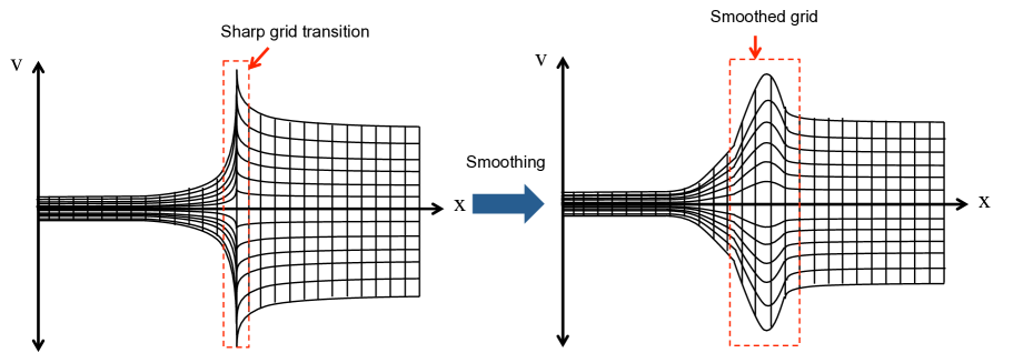
Figure 3.3: Illustration of unsmoothed (left) and smoothed phase-space grid on a plasma shock problem.

4 Numerical results

In this section, we demonstrate the properties of our numerical implementation, both in terms of conservation and order of accuracy, with various examples of varying degrees of complexity. For all problems, we normalize the mass, charge, temperature, density, velocity, and time to the proton mass, $m_{0}$, proton charge, $e$, reference temperature, $T_{0}$, density, $n_{0}$, characteristic speed, $v_{0}=\sqrt{T_{0}/m_{0}}$, and time-scale, $\tau_{0}=\frac{3\sqrt{m_{0}}T_{0}^{3/2}}{4\sqrt{\pi}n_{0}\Lambda e^{4}}$, respectively. A fixed Coulomb logarithm, $\Lambda=10$, is used throughout this study. All normalized distribution functions are initialized as Maxwellians, with prescribed moments in $n$, $u$, and $T$ as:

$$\widehat{f}_{M}=\frac{nv^{*}}{\left(\pi v_{th}^{3}\right)^{3/2}}\textnormal{exp}\left[-\frac{\left(\widehat{v}_{||}v^{*}-u_{,||}\right)^{2}+\left(v^{*}\widehat{v}_{\perp}\right)^{2}}{v_{th}^{2}}\right].$$ (4.1)

The initial normalization velocity profile, $v^{*}(x)$, is found by applying a few binomial smoothing passes, $v^{*}=\textnormal{SM}^{N_{sm}}\left(v_{th}\right)$ (unless otherwise stated, $N_{sm}=5$), such that high wavenumber components of the initial temperature profile (if present) are smoothed out to prevent large numerical errors stemming from the computation of spatial gradients of $v^{*}$ in the inertial term to pollute the accuracy of the solutions. We note that in this study, we use a discrete quadrature error accounting technique to ensure discrete Maxwellian moments agree with prescribed ones [22].

For the solver, we employ an Anderson acceleration scheme [23] with nonlinear elimination strategies for the Rosenbluth potential and fluid electrons (similar to Ref. [14]) and similar preconditioning strategies (multigrid and operator splitting) as discussed in Refs. [14, 24]. Finally, unless otherwise stated, we employ a nonlinear convergence tolerance of $\epsilon_{r}=10^{-3}$.

4.1 Periodic sinusoidal ion-electron temperature equilibration

We begin by demonstrating that our proposed grid adaptivity and discretization strategy recovers Braginskii’s fluid solution in a short mean-free path plasma [15]. Consider an initially stationary proton-electron plasma in hydrodynamic equilibrium with the total pressure, $P=nT=1$, and a sinusoidal temperature profile of $T_{i}=T_{e}=1+0.2\textnormal{sin}\left(k_{x}x\right)$, where $k_{x}=\frac{2\pi}{L_{x}}$ with $L_{x}=1000$ the system size. We consider a domain of $x\in\left[0,L_{x}\right]$ and $\widehat{L}_{||}=\left[-6,6\right]$, $\widehat{L}_{\perp}=[0,6]$ with grids $N_{x}=192$, and $N_{v}=N_{||}\times N_{\perp}=64\times 32$. To test our simulation against theory, we focus on the ion collisional heat flux. The numerical ion thermal conductivity is computed from Fick’s law as

$$\kappa_{i,sim}=-\frac{Q_{||,i}}{\partial T_{i}/\partial x},$$ (4.2)

where

$$Q_{||,i}=\frac{m_{i}}{2}\left\langle\left(v_{||}-u_{||}\right)\left(\mathbf{v}-\mathbf{u}_{i}\right)^{2},f_{i}\right\rangle_{v}.$$

Here, the subscript $i$ denotes ions. This is to be compared with Braginskii’s theoretical result [15]

$$\kappa_{i}=3.9\frac{n_{i}T_{i}\tau_{i}}{m_{i}},$$ (4.3)

where $\tau_{i}=\frac{3\sqrt{m_{i}}T_{i}^{3/2}}{4\sqrt{\pi}n_{i}\Lambda e^{4}}$ is the ion collision time. In Fig. 4.1-left, the Braginskii ion thermal conductivity is plotted for both simulation and theory, and an excellent agreement is found.

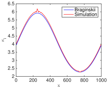
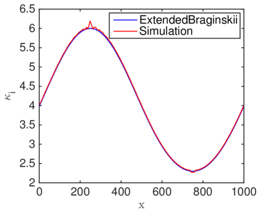
Figure 4.1: Periodic sinusoidal ion-electron temperature equilibration. Braginskii thermal conductivity for protons versus simulation (left) and the same but for a a higher-order truncation in the Laguerre polynomial expansion of Braginskii’s thermal conductivity coefficient (right).

We point out that the computation of $\kappa_{i}$ is a bit noisy at the extrema owing to the vanishing temperature gradient in the denominator of Eq. (4.2). We note that, for the chosen domain size, gradient-scale length, and mean free path, the maximum Knudsen number, $Kn=\lambda_{i,mfp}/L_{T}$, with $L_{T}=T_{i}/\partial_{x}T_{i}$, is $\sim{\cal O}\left(10^{-3}\right)$, making the Braginskii approximation, Eq. (4.3), appropriate. We point out that there is a roughly 2% uniform discrepancy between theory and simulation, which is caused by only retaining two terms in the truncation of the Laguerre polynomial expansion of the distribution function in Braginskii’s result [15]. Fig. 4.1-right depicts a comparison with the analytical result when three terms in the expansion are retained, removing the discrepancy.

We examine next the quality of the conservation properties with varying nonlinear convergence tolerance; refer to Fig. 4.2.

Figure 4.2: Periodic sinusoidal ion-electron temperature equilibration. Conservation of mass (left), momentum (middle), and energy (right) versus time for varying nonlinear convergence tolerance, $\epsilon_{r}$.

Here,

$$\frac{\Delta M}{M^{0}}=\left|\frac{\int_{L_{min}}^{L_{max}}dx\left[\left\langle 1,\widehat{f}\right\rangle_{\mathbf{\widehat{v}}}-\left\langle 1,\widehat{f}^{0}\right\rangle_{\mathbf{\widehat{v}}}\right]}{\int_{L_{min}}^{L_{max}}dx\left\langle 1,\widehat{f}^{0}\right\rangle_{\mathbf{\widehat{v}}}}\right|,$$

$$\Delta I=\left|\int_{L_{min}}^{L_{max}}dx\left[\left\langle\widehat{v}_{||}v^{*},\widehat{f}\right\rangle_{\mathbf{\widehat{v}}}-\left\langle\widehat{v}_{||}v^{*,0},\widehat{f}^{0}\right\rangle_{\mathbf{\widehat{v}}}\right]\right|,$$

and

$$\frac{\Delta U}{U_{0}}=\left|\frac{\int_{L_{min}}^{L_{max}}dx\left\{\left[m\left\langle\frac{\widehat{v}^{2}\left(v^{*}\right)^{2}}{2},\widehat{f}\right\rangle_{\mathbf{\widehat{v}}}+\frac{3}{2}n_{e}T_{e}\right]-\left[m\left\langle\frac{\widehat{v}^{2}\left(v^{*,0}\right)^{2}}{2},\widehat{f}^{0}\right\rangle_{\mathbf{\widehat{v}}}+\frac{3}{2}n_{e}^{0}T_{e}^{0}\right]\right\}}{\int_{L_{min}}^{L_{max}}dx\left[m\left\langle\frac{\widehat{v}^{2}\left(v^{*,0}\right)^{2}}{2},\widehat{f}^{0}\right\rangle_{\mathbf{\widehat{v}}}+\frac{3}{2}n_{e}^{0}T_{e}^{0}\right]}\right|$$

are the measures of discrete conservation error in mass, momentum, and energy, respectively. As can be seen, the conservation quality improves with tighter nonlinear convergence tolerances, as expected.

Using this test example, we demonstrate next that our proposed scheme is second-order accurate in configuration space, velocity space, and time. We remark that, owing to the velocity-space adaptivity, it is unsuitable to use the $L_{2}$-norm of the distribution function,

$$L_{2}=\sum_{\alpha=1}^{N_{s}}\sqrt{\text{$\int$dx}\int dv\left(f_{\alpha}-f_{\alpha}^{ref}\right)^{2}},$$ (4.4)

to quantify the error, because $f_{\alpha}^{\Delta t}=\left(v_{\alpha}^{*,\Delta t}\right)^{-3}\widehat{f}\left(v_{\alpha}^{*,\Delta t}\widehat{v}\right)$ and $f_{\alpha}^{\Delta t,ref}=\left(v_{\alpha}^{*,\Delta t,ref}\right)^{-3}\widehat{f}\left(v_{\alpha}^{*,\Delta t,ref}\widehat{v}\right)$ live on different spatial meshes (where the superscripts $\Delta$t and $\Delta t,ref$ correspond to a prescribed time-step size and a time-step size for the reference solution, respectively). We recall, that this difference in the mesh stems from the fact that the velocity space is normalized by $v^{*}$, which is lagged by a time-step and undergoes a smoothing operation. As a proxy measure of the numerical error, which is much simpler to compute and is independent of a normalization choice, we consider the temperature.

To demonstrate the second-order temporal convergence of the BDF2 scheme, we compute a relative difference of the temperature with respect to a reference temperature,

$${\cal E}_{T}^{\Delta t}=\sum_{i=1}^{N_{x}}\Delta x\sum_{\alpha=1}^{N_{s}}\frac{\left|T_{\alpha,i}^{\Delta t,ref}-T_{\alpha,i}^{\Delta t}\right|}{T_{\alpha,i}^{\Delta t,ref}}.$$ (4.5)

Here, $T^{\Delta t,ref}$ is the reference temperature solution obtained using a reference time-step size ($\Delta t_{ref}=10^{-4})$ at the final time $t_{max}=1$. For all cases, we use a grid size of $N_{x}=24$ and $N_{v}=64\times 32$ and a nonlinear convergence tolerance of $\epsilon_{r}=10^{-8}$ (to adequately capture small signals for small $\Delta t$). Fig. 4.3-left shows that the expected order of accuracy with $\Delta t$ refinement is confirmed.

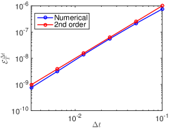
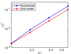
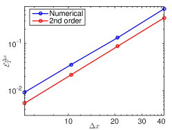
Figure 4.3: Periodic sinusoidal ion-electron temperature equilibration. On the left, we demonstrate a second-order convergence with time-step refinement. At the center, we demonstrate a second-order convergence with velocity-space refinement. On the right, we demonstrate a second-order convergence with physical-space refinement.

Second-order accuracy in velocity-space is demonstrated similarly by computing:

$${\cal E}_{T}^{\Delta\widehat{v}}=\sum_{i=1}^{N_{x}}\Delta x\sum_{\alpha=1}^{N_{s}}\frac{\left|T_{\alpha,i}^{\Delta\widehat{v},ref}-T_{\alpha,i}^{\Delta\widehat{v}}\right|}{T_{\alpha,i}^{\Delta\widehat{v},ref}}.$$ (4.6)

Here, $T^{\Delta\widehat{v},ref}$ is the reference temperature solution obtained using a reference grid resolution of $N_{v}^{ref}=512\times 256$. A uniform grid refinement is performed in both velocity-space directions. For all cases, we use $\Delta t=1$ and a final time $t_{max}=10$ with $N_{x}=96$. Fig. 4.3-center confirms second-order convergence with $\Delta\widehat{v}$ refinement.

Finally, to demonstrate second-order accuracy of the spatial discretization, we use a similar approach and compute

$${\cal E}_{T}^{\Delta x}=\sum_{i=1}^{N_{x,ref}}\Delta x_{ref}\sum_{\alpha=1}^{N_{s}}\frac{\left|T_{\alpha,i}^{\Delta x,ref}-T_{\alpha,i}^{\Delta x}\right|}{T_{\alpha,i}^{\Delta x,ref}}.$$ (4.7)

Here, $T^{\Delta x,ref}$ is the reference-temperature solution obtained using a reference-grid resolution ($N_{x,ref}=768)$ with a final time $t_{max}=1$. To compute the norm in Eq. (4.7), we interpolate the coarse solution onto the fine grid via a $4^{th}$ order spline. For all cases, we use a velocity space grid size of $N_{v}=32\times 16$. Fig. 4.3-right confirms the expected order of accuracy of our spatial discretization.

4.2 Ion temperature relaxation with an initial periodic hyperbolic tangent profile

This example highlights the importance of enforcing discrete conservation in the Vlasov equation when gradients (both in physical and velocity space) are marginally resolved. We consider a single ion species with $m=1$, $q=1$, without electrons, on a periodic spatial domain of $L_{x}\in\left[-50,50\right]$, and a velocity domain $\widehat{L}_{||}\in\left[-6,6\right]$, $\widehat{L}_{\perp}\in\left[0,5\right]$. We consider a mesh of $N_{x}=96$ and $N_{v}=64\times 32$. We assume an initially stationary distribution, $u=0$, with a homogeneous density, $n=1$, and a hyperbolic tangent temperature profile,

$$T=0.495\begin{cases}1+\textnormal{tanh}\left(\chi\left[x+25\right]\right)+b_{T0}&\textnormal{if}\;-50\leq x\leq 0\\ 1-\textnormal{tanh}\left(\chi\left[x-25\right]\right)+b_{T1}&\textnormal{otherwise}\end{cases}.$$

Here, $\chi$ is a parameter that controls the gradient scale length of the hyperbolic tangent; values for $\chi$ are provided later. We remark, that for these parameters, $v_{th,max}/v_{th,min}=\text{$\sqrt{T_{max}/T_{min}}$}=10$ and a static uniform grid will require on order of $(v_{th,max}/v_{th,min})^{2}=100$ times more grid points than our velocity adaptivity strategy to resolve the cold distribution function adequately.

We investigate the impact of a lack of conservation on long-term accuracy with respect to various parameters. We turn off the conservation scheme for the inertial term arising from the spatial dependence of $v^{*}$. We demonstrate first that the quality of conservation depends on grid resolution. We choose $\chi$ equal to $0.5$, $1$, and $10$ without ensuring either momentum nor energy conservation symmetries for this inertial term. In Fig. 4.4, we show the solution profile for all $\chi$ and $N_{sm}=0$ at $t\approx 1700$.

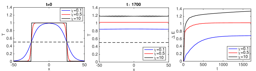
Figure 4.4: Ion temperature relaxation with an initial periodic hyperbolic tangent profile. The quality of solution for different $\chi$ and $N_{sm}=0$ at $t=0$ (left) and $t\approx 1700$ (center). The dashed black line is the analytical equilibrium solution. The energy conservation error is shown on the right

As can be seen, in all cases a large energy conservation error is accumulated over time, leading to significant numerical heating. For the $\chi=10$ case, the initial numerical heating coming from the sharp gradients is strong enough that a grid-scale mode is excited.

Numerical accuracy is improved by either increasing velocity space resolution or by smoothing $v^{*}$ (as the spatial inertial term vanishes in the limit of $\partial_{x}v^{*}=0$). We recall that the introduction of $v^{*}$ is simply a numerical trick and that the smoothing of $v^{*}$ does not change the physics of the problem. In Fig. 4.5, we show the impact of varying $N_{sm}$ on the quality of energy conservation, with the quality improving for enhanced smoothing of $v^{*}$, as expected.

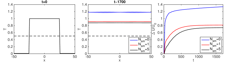
Figure 4.5: Ion temperature relaxation with an initial periodic hyperbolic tangent profile. The quality of solution for a varying number of binomial smoothing iterations, $N_{sm}$, on $v^{*}$ at $t=0$ (left) and $t\approx 1700$ (center). The dashed black line is the analytical equilibrium solution. The energy conservation error is shown on the right

Next, we investigate the impact of increasing velocity-space resolution with $N_{x}=96$, $\chi=10$, and $N_{sm}=5$. In Fig. 4.6, we show the solution profile for different velocity-space grids.

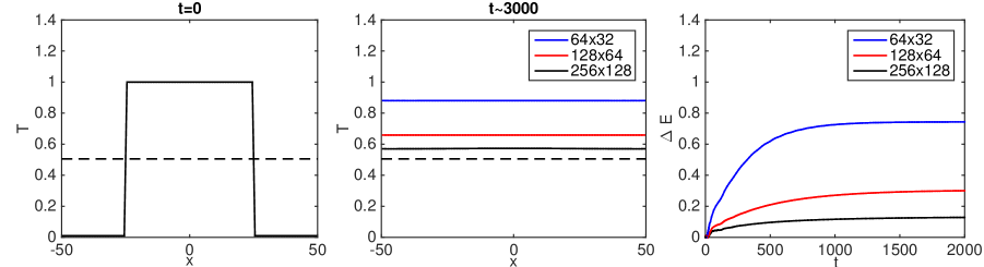
Figure 4.6: Ion temperature relaxation with an initial periodic hyperbolic tangent profile. The quality of solution for varying velocity-space grid resolution at $t=0$ (left) and $t\approx 3000$ (center). The dashed black line is the analytical equilibrium solution. The energy conservation error is shown on the right

As can be seen, a grid of $N_{v}=256\times 128$ is required to reduce the energy conservation error to within $10\%$. At this point, the error in conservation is mostly dominated by configuration space discretization errors (due to the spatial interpolation procedure embedded in the definition of the conservation symmetries, Eq. (3.34) and (3.56)), and further improvement in conservation via refinement in velocity space will require refinement in configuration space.

Finally, we show that by ensuring the conservation symmetries in the inertial term, the numerical heating effect can be suppressed to nonlinear convergence tolerance even with coarser grids. We employ a grid of $N_{x}=96$ and $N_{v}=64\times 32$, $\chi=10$ and $N_{sm}=5$; refer to Fig. 4.7. The correct asymptotic solution is obtained. Conservation errors are kept small throughout the simulation and commensurate with the default nonlinear relative convergence tolerance ($10^{-3}$).

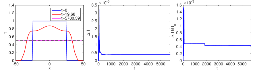
Figure 4.7: Ion temperature relaxation with an initial periodic hyperbolic tangent profile. The solution is obtained by enforcing the discrete Vlasov spatial inertial conservation symmetries in Eqs. (3.52) to (3.56) (left). The dashed black line is the analytical equilibrium solution. Total momentum and energy conservation error is shown in the center and right, respectively.

4.3 Mach 5 steady-state shock

We simulate a Mach 5 shock in a proton-electron plasma in the frame of the shock. The purpose of this test problem is to demonstrate that the correct steady-state solution is obtained for a non-trivial problem. We obtain the hydrodynamic jump conditions from the Hugoniot relationship:

$$\frac{P_{1}}{P_{0}}=\frac{2\gamma M^{2}-(\gamma-1)}{\gamma+1},$$ (4.8)

$$\frac{\rho_{1}}{\rho_{0}}=\frac{u_{0}}{u_{1}}=\frac{M^{2}\left(\gamma+1\right)}{M^{2}\left(\gamma-1\right)+2}.$$ (4.9)

Here, the subscript $0$ denotes the upstream (un-shocked) region and $1$ denotes the downstream (shocked) region. Combining these equations gives:

$$\frac{u_{0}}{u_{1}}=\frac{\left(\gamma-1\right)P_{0}+\left(\gamma+1\right)P_{1}}{\left(\gamma+1\right)P_{0}+\left(\gamma-1\right)P_{1}}.$$ (4.10)

Here, $\gamma$ is the specific heat ratio ($\gamma=5/3$ for fully ionized plasmas), $P$ is the total static pressure (i.e., $P=P_{i}+P_{e}$), $\rho=\sum_{\alpha=1}^{N_{s}}m_{\alpha}n_{\alpha}$ is the total mass density, and $u=\sum_{\alpha=1}^{N_{s}}m_{\alpha}n_{\alpha}u_{\alpha}/\sum_{\alpha=1}^{N_{s}}m_{\alpha}n_{\alpha}$ is the mass averaged drift velocity of the respective regions. The upstream velocity can be expressed as

$$u_{0}=Mc_{0},$$ (4.11)

where $c_{0}$ is the upstream sound speed,

$$c_{0}=\sqrt{\gamma\frac{P_{0}}{\rho_{0}}}.$$ (4.12)

Employing the downstream condition of $\rho_{1}=mn_{1}=1,$ $n_{1}=1$, $m_{1}=1$, $P_{1}=P_{1,i}+P_{1,e}=2P_{1,i}=2n_{1,i}T_{1,i}=2$, $T_{1,i}=1$, and $M=5$ gives for the upstream conditions $\rho_{0}=mn_{0}=0.28$, $P_{0}=0.1290$, and $T_{0}=0.1152$ . Then, $c_{0}=0.619697$, $u_{0}=Mc_{0}=3.0984$, and $u_{1}=0.8676$.

We consider a computational domain of $L_{x}\in\left[0,160\right]$, $\widehat{L}_{||}\in\left[-4,13\right]$, $\widehat{L}_{\perp}\in\left[0,6\right]$ with a grid of $N_{x}=96$, $N_{v}=128\times 64$. The solution is initialized with

$$n=\begin{cases}0.28&\textnormal{if}\;x\leq 80\\ 1&\textnormal{otherwise}\end{cases},\;u=\begin{cases}3.0984&\textnormal{if}\;x\leq 80\\ 0.8676&\textnormal{otherwise}\end{cases},\;T=\begin{cases}0.1152&\textnormal{if}\;x\leq 80\\ 1&\textnormal{otherwise}\end{cases}.$$ (4.13)

In the configuration space, we consider in-flow and out-flow boundary conditions for the ion distribution functions:

$$f_{B}\left(v_{||},v_{\perp}\right)=\begin{cases}f_{M}\left(n_{B},u_{B},T_{B}\right)&\textnormal{if}\;\widehat{l}_{B}v_{||}\leq 0\\ f_{C}&\textnormal{otherwise}\end{cases}.$$ (4.14)

Here, $n_{B}$, $u_{B}$, and $T_{B}$ are the moments defined by the Hugoniot conditions at the boundary, $\widehat{l}_{B}$ is the $x$-component of the boundary surface normal vector ($\pm 1$ in 1D), and $f_{C}$ is the distribution function defined in the computational cell adjacent to the boundary. For the fluid electron temperature, we use the Dirichlet boundary conditions to impose the Hugoniot asymptotic jump.

The simulation is run for $t_{max}=250$ until transient structures have equilibrated.

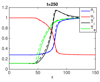
Figure 4.8: Mach 5 steady-state shock. The solid lines are from our simulation, while the dashed lines are from Ref. [25] for a similar setup (data points were manually extracted from Fig 2.a in Ref. [25] using the WebPlotDigitizer software [26]). We note, that in the plot, the drift velocity, $u$, is normalized to the upstream value. Additionally, the x-axis was scaled by a factor of $\frac{\sqrt{2}}{3\pi}$ to convert the data from [25] to our normalization.

A very good agreement is found with respect to the reference solution [25]; refer to Fig. 4.8.

4.4 Shock interaction with a density jump

In this example, we simulate a shock propagating through a mass-density discontinuity. Unlike the standing shock case, where a steady-state solution can be found, this problem is inherently dynamic and tests the robustness of the overall approach. The analytical solution is well-iknown and given in App. E for reference. We test our approach against this solution.

We consider an $M=5$ shock propagating from left to right through a plasma comprised of protons on the left and deuterons on the right. The ions are initially in pressure equilibrium at the mass-density-jump interface; refer to Fig 4.9.

Figure 4.9: Shock interaction with a density jump. Illustration of the problem setup before (left) and after (right) shock breakout through the interface.

The problem is simulated in a domain of $L_{x}\in\left[0,2500\right]$, $\widehat{L}_{||}\in\left[-7,7\right]$, and $\widehat{L}_{\perp}\in\left[0,7\right]$, on a grid of $N_{x}=192$ and $N_{v}=128\times 64$, with in-/out-flow boundary conditions in the configuration space for the ion-distribution functions and Dirichlet boundary conditions for fluid-electron temperature. The initial conditions are, for protons,

$$n_{P}=\begin{cases}n_{P0}&\textnormal{if}\;0\leq x<x_{0}\\ n_{P1}&\textnormal{if}\;x_{0}\leq x<x_{1}\\ n_{P2}&\textnormal{otherwise}\end{cases},\;u_{P}=\begin{cases}u_{P0}&\textnormal{if}\;0\leq x<x_{0}\\ 0&\textnormal{otherwise}\end{cases},\;T_{P}=\begin{cases}T_{P0}&\textnormal{if}\;0\leq x<x_{0}\\ T_{P1}&\textnormal{otherwise}\end{cases},$$ (4.15)

for deuterons,

$$n_{D}=\begin{cases}n_{D0}&\textnormal{if}\;0\leq x<x_{0}\\ n_{D1}&\textnormal{otherwise}\end{cases},\;u_{D}=\begin{cases}u_{D0}&\textnormal{if}\;0\leq x<x_{0}\\ 0&\textnormal{otherwise}\end{cases},\;T_{D}=\begin{cases}T_{D0}&\textnormal{if}\;0\leq x<x_{0}\\ T_{D1}&\textnormal{otherwise}\end{cases},$$ (4.16)

and electron temperature,

$$T_{e}=\begin{cases}T_{e0}&\textnormal{if}\;0\leq x<x_{0}\\ T_{e1}&\textnormal{otherwise}\end{cases}.$$ (4.17)

Here, $x_{0}=150$ and $x_{1}=250$, $n_{P0}=1$, $n_{P1}=0.28$, $n_{P2}=0.005$, $n_{D0}=0.0028$, $n_{D1}=0.28$, $u_{P0}=u_{D0}=2.2308$, $T_{P0}=T_{D0}=T_{e0}=1$, and $T_{P1}=T_{D1}=T_{e1}=0.1152$. We use the initial conditions at the boundary to provide the in-flow conditions for ions and Dirichlet conditions for electrons.

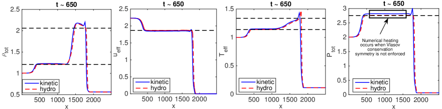
Figure 4.10: Shock interaction with a density jump. From left to right, we show the total hydrodynamic mass density, $\rho_{tot}=\sum_{\alpha}^{N_{s}}m_{\alpha}n_{\alpha}$, the center of mass velocity, $u_{eff}=\sum_{\alpha}^{N_{s}}m_{\alpha}n_{\alpha}u_{\alpha}/\rho_{tot}$, the effective ion temperature, $T_{eff}=\sum_{\alpha}^{N_{s}}n_{\alpha}T_{\alpha}/\sum_{\alpha}^{N_{s}}n_{\alpha}$, and the total pressure, $P_{tot}=\left(\sum_{\alpha}^{N_{s}}n_{\alpha}T_{\alpha}+n_{e}T_{e}\right)$. The top row represents the case with all conservation symmetries enforced and the bottom without enforcing the Vlasov conservation symmetries. Here, the blue lines represent the solution obtained from our kinetic code, while the red lines show the solution obtained from a hydro code. As can be seen, our implementation with grid adaptivity and discrete conservation strategy correctly recovers the shock jump conditions (black dashed lines) across the density jump, while numerical heating is observed when the Vlasov conservation symmetries are not enforced.

As can be seen in Fig. 4.10, the long term kinetic solution agrees very well with a hydro simulation (obtained from an in-house multi-fluid Euler code), demonstrating the capability of the proposed approach to capture the hydrodynamic limit. We stress that this limit is rigorously obtained by ensuring strict conservation. The bottom row of Fig. 4.10 shows that numerical heating –result of not enforcing the conservation symmetry for the Vlasov operator– results in the pressure in the solution departing from the correct asymptotics (~5% error for the current grid). While this error may seem small (a consequence of this problem setup being much more constrained than the periodic case), its impact in highly nonlinear applications could be very large (for instance, in inertial confinement fusion, up to 4 shocks are used to compress and heat the fuel to fusion conditions, and this level of numerical heating can result in a ~20% error in the final fuel temperature, significantly altering implosion dynamics).

5 Conclusion

In this study, we have demonstrated, for the first time, an approach that is fully conservative and optimally adaptive for the multi-species, 1D2V VFP ion plasma equations with fluid electrons. The approach features exact (in practice, up to a nonlinear tolerance) mass, momentum, and energy conservation and allows for a large temperature variation in time and in space. Our approach analytically adapts the velocity-space mesh for each species by normalizing the velocity space to each species reference velocity, $v^{*}$ (i.e., we consider multiple velocity-space grids). The analytical formulation allows us to expose the continuum-conservation symmetries in the inertial terms arising from the normalization, which are then enforced discretely via the use of nonlinear constraints, as proposed in earlier studies [27, 14]. We have demonstrated the ability of the scheme to capture transport and hydrodynamic asymptotic solutions correctly, which is exceedingly challenging for VFP codes.

We remark that the present approach cannot handle well situations where the bulk velocity is much larger than the thermal velocity of the plasma. In these situations, one must shift the velocity space by the bulk velocity, as was done in Ref. [8]. This will give rise to an additional inertial term, which will be considered in future work. We close by noting that the methodology developed in this study has been extended to a spherical geometry with grid adaptivity in configuration space. This work will be documented in a follow-on manuscript.

Appendix A Details on the fluid-electron model

The frictional force between the $\alpha$-ion species and electrons is given as,

$$\mathbf{F}_{\alpha e}=-m_{e}n_{e}\nu_{e\alpha}\left(\mathbf{u}_{\alpha}-\left\langle\mathbf{u}_{\alpha}\right\rangle\right)+\alpha_{0}m_{e}n_{e}\nu_{e\alpha}\left(\mathbf{u}_{e}-\left\langle\mathbf{u}_{\alpha}\right\rangle\right)+\beta_{0}\frac{n_{e}\nu_{e\alpha}\nabla T_{e}}{\sum_{\alpha}^{N_{s}}\nu_{e\alpha}},$$ (A.1)

where

$$\left\langle\mathbf{u}_{\alpha}\right\rangle\equiv\frac{\sum_{\alpha}^{N_{s}}\nu_{e\alpha}\mathbf{u}_{\alpha}}{\sum_{\alpha}^{N_{s}}\nu_{e\alpha}},$$ (A.2)

$$\nu_{e\alpha}=\frac{4\sqrt{2\pi}n_{\alpha}q_{\alpha}^{2}e^{4}\Lambda_{e\alpha}}{3\sqrt{m_{e}}T_{e}^{3/2}},$$ (A.3)

$$\alpha_{0}=\frac{4\left(16Z_{eff}^{2}+61\sqrt{2}Z_{eff}+72\right)}{217Z_{eff}^{2}+604\sqrt{2}Z_{eff}+288},$$ (A.4)

$$\beta_{0}=\frac{30Z_{eff}\left(11Z_{eff}+15\sqrt{2}\right)}{217Z_{eff}^{2}+604\sqrt{2}Z_{eff}+288},$$ (A.5)

and the effective charge is defined as

$$Z_{eff}=-\frac{\sum_{\alpha}^{N_{s}}q_{\alpha}^{2}n_{\alpha}}{q_{e}n_{e}}.$$ (A.6)

The electron heat flux is given as

$$\mathbf{Q}_{e}=\beta_{0}n_{e}T_{e}\left(\mathbf{u}_{e}-\left\langle\mathbf{u}_{\alpha}\right\rangle\right)-\kappa_{e}\nabla T_{e},$$ (A.7)

where the electron-thermal conductivity is given as

$$\kappa_{e}=\frac{\gamma_{0}n_{e}T_{e}}{m_{e}\sum_{\alpha}^{N_{s}}\nu_{e\alpha}},$$ (A.8)

with

$$\gamma_{0}=\frac{25Z_{eff}\left(433Z_{eff}+180\sqrt{2}\right)}{4\left(217Z_{eff}^{2}+604\sqrt{2}Z_{eff}+288\right)}.$$ (A.9)

See Ref. [16] for a complete derivation and discussion of the coefficients $\alpha_{0}$, $\beta_{0}$, and $\gamma_{0}$.

Appendix B Vlasov-Fokker-Planck equation expressed in normalized velocity variables

We consider the Vlasov equation under the velocity coordinate transformation $\mathbf{v}=v_{\alpha}^{*}\left(x,t\right)\widehat{\mathbf{v}}$. The total derivative of $\widehat{f}_{\alpha}\left(x,\widehat{v},t\right)$ keeping $x$ and $\mathbf{v}$ constant is given by

$$\left.\partial_{t}\widehat{f}_{\alpha}\right|_{x,\mathbf{v}}=\left.\partial_{t}\widehat{f}_{\alpha}\right|_{x,\mathbf{\widehat{v}}}+\left.\partial_{t}\mathbf{\widehat{v}}\right|_{x,\mathbf{v}}\cdot\left.\frac{\partial\widehat{f}_{\alpha}}{\partial\mathbf{\widehat{v}}}\right|_{x,\mathbf{v}},$$ (B.1)

where $\left.\partial_{t}\mathbf{\widehat{v}}\right|_{x,\mathbf{v}}$ can be expressed as

$$\left.\partial_{t}\mathbf{\widehat{v}}\right|_{x,\mathbf{v}}=-\frac{\mathbf{\widehat{v}}}{v_{\alpha}^{*}}\partial_{t}v_{\alpha}^{*}.$$ (B.2)

There results

$$\left.\partial_{t}\widehat{f}_{\alpha}\right|_{x,\mathbf{v}}=\left.\partial_{t}\widehat{f}_{\alpha}\right|_{x,\mathbf{\widehat{v}}}-\frac{\partial_{t}v_{\alpha}^{*}}{v_{\alpha}^{*}}\mathbf{\widehat{v}}\cdot\widehat{\nabla}_{v}\widehat{f}_{\alpha}.$$ (B.3)

Similarly, we have

$$\left.\partial_{x}\widehat{f}_{\alpha}\right|_{t,\mathbf{v}}=\left.\partial_{x}\widehat{f}_{\alpha}\right|_{t,\mathbf{\widehat{v}}}+\left.\partial_{x}\mathbf{\widehat{v}}\right|_{t,\mathbf{v}}\cdot\widehat{\nabla}_{v}\widehat{f}_{\alpha},$$

where

$$\left.\partial_{x}\mathbf{\widehat{v}}\right|_{t,\mathbf{v}}=-\frac{\mathbf{\widehat{v}}}{v_{\alpha}^{*}}\partial_{x}v_{\alpha}^{*}.$$

Therefore

$$\left.\partial_{x}\widehat{f}_{\alpha}\right|_{t,\mathbf{v}}=\left.\partial_{x}\widehat{f}_{\alpha}\right|_{t,\mathbf{\widehat{v}}}-\frac{\partial_{x}v_{\alpha}^{*}}{v_{\alpha}^{*}}\mathbf{\widehat{v}}\cdot\widehat{\nabla}_{v}\widehat{f}_{\alpha}.$$

From the Vlasov equation we have

$$\left.\partial_{t}f_{\alpha}\right|_{x,\mathbf{v}}+\partial_{x}\left.\left(v_{||}f_{\alpha}\right)\right|_{\mathbf{v},t}=\left.\partial_{t}\left[\frac{\hat{f}_{\alpha}}{\left(v_{\alpha}^{*}\right)^{3}}\right]\right|_{x,\mathbf{v}}+v_{\parallel}\partial_{x}\left.\left[\frac{\widehat{f}_{\alpha}}{\left(v_{\alpha}^{*}\right)^{3}}\right]\right|_{t,\mathbf{v}} =$$

$$\left[\frac{\left.\partial_{t}\hat{f}_{\alpha}\right|_{x,\mathbf{v}}}{\left(v_{\alpha}^{*}\right)^{3}}+\hat{f}_{\alpha}\partial_{t}\left.(v_{\alpha}^{*})^{-3}\right|_{x}\right]+v_{\parallel}\left[\frac{\left.\partial_{x}\widehat{f}_{\alpha}\right|_{t,\mathbf{v}}}{\left(v_{\alpha}^{*}\right)^{3}}+\widehat{f}_{\alpha}\partial_{x}\left.\left(v_{\alpha}^{*}\right)^{-3}\right|_{t}\right] =$$

$$\frac{1}{\left(v_{\alpha}^{*}\right)^{3}}\left[\partial_{t}\left.\widehat{f}_{\alpha}\right|_{x,\mathbf{\widehat{v}}}-\frac{\left(\partial_{t}v_{\alpha}^{*}+v_{\parallel}\partial_{x}v_{\alpha}^{*}\right)}{v_{\alpha}^{*}}\mathbf{\widehat{v}}\cdot\widehat{\nabla}_{v}\widehat{f}_{\alpha}-\frac{3\widehat{f}_{\alpha}}{v_{\alpha}^{*}}\left(\partial_{t}v_{\alpha}^{*}+v_{\parallel}\partial_{x}v_{\alpha}^{*}\right)+\hat{v}_{\parallel}v_{\alpha}^{*}\left.\partial_{x}\widehat{f}_{\alpha}\right|_{t,\mathbf{\widehat{v}}}\right] =$$

$$\frac{1}{\left(v_{\alpha}^{*}\right)^{3}}\left[\partial_{t}\left.\widehat{f}_{\alpha}\right|_{x,\mathbf{\widehat{v}}}-\frac{3\widehat{f}_{\alpha}+\mathbf{\widehat{v}}\cdot\widehat{\nabla}_{v}\widehat{f}_{\alpha}}{v_{\alpha}^{*}}\left(\partial_{t}v_{\alpha}^{*}+v_{\parallel}\partial_{x}v_{\alpha}^{*}\right)+\left(\left.\partial_{x}(v_{\alpha}^{*}\hat{v}_{\parallel}\widehat{f}_{\alpha})\right|_{t,\mathbf{\widehat{v}}}-\hat{v}_{\parallel}\widehat{f}_{\alpha}\partial_{x}v_{\alpha}^{*}\right)\right]$$ .

Using $\hat{\nabla}_{\widehat{v}}\cdot\hat{\mathbf{v}}=3$ and $\widehat{\nabla}_{\widehat{v}}\cdot\left(\widehat{v}_{||}\mathbf{\widehat{v}}\right)=4\widehat{v}_{||}$, we find

$$\left.\partial_{t}f_{\alpha}\right|_{x,\mathbf{v}}+\partial_{x}\left.\left(v_{||}f_{\alpha}\right)\right|_{\mathbf{v},t}=\frac{1}{\left(v_{\alpha}^{*}\right)^{3}}\left[\left.\partial_{t}\hat{f}_{\alpha}\right|_{x,\hat{\mathbf{v}}}-\frac{1}{v_{\alpha}^{*}}\frac{\partial v_{\alpha}^{*}}{\partial t}\widehat{\nabla}_{\widehat{v}}\cdot(\mathbf{\widehat{v}}\hat{f}_{\alpha})-\partial_{x}v_{\alpha}^{*}\widehat{\nabla}_{\widehat{v}}\cdot\left(\mathbf{\widehat{v}}\widehat{v}_{||}\widehat{f}_{\alpha}\right)+\partial_{x}\left.\left(v_{\alpha}^{*}\widehat{v}_{||}\widehat{f}_{\alpha}\right)\right|_{t,\mathbf{\widehat{v}}}\right].$$ (B.4)

Finally, the electrostatic-acceleration term is written as

$$\frac{q_{\alpha}}{m_{\alpha}}E_{||}\partial_{v_{||}}f_{\alpha}=\frac{q_{\alpha}}{m_{\alpha}}\frac{E_{||}}{\left(v_{\alpha}^{*}\right)^{4}}\partial_{\widehat{v}_{||}}\widehat{f}_{\alpha}.$$ (B.5)

Substituting these results into the original Vlasov equation, Eq. (2.10), there results the following transformed equation for $\widehat{f}_{\alpha}\left(x,\mathbf{\widehat{v}},t\right)$

$$\partial_{t}\widehat{f}_{\alpha}+\partial_{x}\left(v_{\alpha}^{*}\widehat{v}_{||}\widehat{f}_{\alpha}\right) + \left(\frac{q_{\alpha}}{m_{\alpha}}\frac{E_{||}}{v_{\alpha}^{*}}\right)\partial_{\widehat{v}_{||}}\widehat{f}_{\alpha}-\left(\frac{\partial_{t}v_{\alpha}^{*}}{v_{\alpha}^{*}}\right)\widehat{\nabla}_{v}\cdot\left(\mathbf{\widehat{v}}\widehat{f}_{\alpha}\right)-\left(\partial_{x}v_{\alpha}^{*}\right)\widehat{\nabla}_{v}\cdot\left(\mathbf{\widehat{v}}\widehat{v}_{||}\widehat{f}_{\alpha}\right)$$ (B.6)

$$= \left(v_{\alpha}^{*}\right)^{3}\left(\sum_{\beta}C_{\alpha\beta}+C_{\alpha e}\right)=\sum_{\beta}\widehat{C}_{\alpha\beta}+\widehat{C}_{\alpha e},$$

where we have used the definition of the normalized collision operator, $\hat{C}_{\alpha\beta}=\left(v_{\alpha}^{*}\right)^{3}C_{\alpha\beta}$ [13].

Appendix C Details on discrete conservation strategy for collisions between kinetic ions and fluid electrons

In Sec. 3.4, we introduced the following nonlinear conservation constraints

$$\gamma_{G,\alpha e}=1+\sum_{l=0}^{N_{B}}C_{l}^{G,\alpha e}P_{l}^{G,\alpha e},\;\gamma_{H,\alpha e,u}=1+\sum_{l=0}^{N_{B}}C_{l}^{H,\alpha e,u}P_{l}^{H,\alpha e,u},\;\gamma_{H,\alpha e,F}=1+\sum_{l=0}^{N_{B}}C_{l}^{H,\alpha e,F}P_{l}^{H,\alpha e,F}$$ (C.1)

to discretely ensure the conservation symmetries for the ion-electron collision operator [Eqs. (2.28), (2.29), (2.30), (2.35), (2.36), (2.37)]. Here, $C_{l}$ and $P_{l}$ are the coefficients and corresponding basis functions that will be used to ensure the conservation symmetries. In this study, we use the Fourier basis in both $v_{||}$ and $v_{\perp}$ directions,

$$\sum_{l=0}^{N_{b}}P_{l}\equiv\sum_{l_{||}=0}^{N_{B,||}}P_{l_{||}}\left(v_{||}\right)\sum_{l_{\perp}=0}^{N_{B,\perp}}P_{l_{\perp}}\left(v_{\perp}\right)$$ (C.2)

where

$$P_{l_{||}}=\begin{cases}1&\text{{if}}\;l_{||}=0\\ \textnormal{sin}\left[l_{||}k_{||}v_{||}\right]&\textnormal{if}\;\textnormal{mod}\left(l_{||},2\right)=0\\ \textnormal{cos}\left[(l_{||}-1)k_{||}v_{||}\right]&\textnormal{if}\;\textnormal{mod}\left(l_{||},2\right)=1\end{cases}$$ (C.3)

$$P_{l_{\perp}}=\begin{cases}1&\text{{if}}\;l_{\perp}=0\\ \textnormal{sin}\left[l_{\perp}k_{\perp}v_{\perp}\right]&\textnormal{if}\;\textnormal{mod}\left(l_{\perp},2\right)=0\\ \textnormal{cos}\left[(l_{\perp}-1)k_{\perp}v_{\perp}\right]&\textnormal{if}\;\textnormal{mod}\left(l_{\perp},2\right)=1\end{cases}$$ (C.4)

and $k_{||}=2\pi/L_{||},\;k_{\perp}=2\pi/L_{\perp}$ are the wave vectors. We also choose $l_{||}=l_{\perp}=\left(0,1,2\right)$. The coefficients are obtained by solving a constrained-minimization problem for the following objective functions:

$$F\left(\mathbf{C}^{q},\mathbf{\lambda}_{q}\right)=\frac{1}{2}\sum_{l=0}^{N}C_{l}^{q}-\boldsymbol{\lambda}_{q}^{T}\cdot\mathbf{M}_{q},\textnormal{ where }q=G,\;u,\;F_{\alpha e},$$ (C.5)

which satisfies the continuum symmetries in Eqs. (2.28), (2.29), (2.30), (2.35), (2.36), (2.37). Here, $\mathbf{\lambda}$ is the vector of Lagrange multipliers and $\mathbf{M}$ is the vector of vanishing constraints that ensures the following discrete-momentum and energy-conservation symmetries for the ion-electron-collision operator:

$$\mathbf{M}_{G}=\begin{bmatrix}m_{\alpha}\left\langle v_{||},\Gamma_{\alpha e}\nabla_{v}\cdot\left[\gamma_{G}\stackrel{{\scriptstyle\leftrightarrow}}{{\mathsfsl{D}}}_{\alpha e}\cdot\nabla_{v}f_{\alpha}\right]\right\rangle_{\mathbf{v}}\\ \Gamma_{\alpha e}m_{\alpha}\left\langle\frac{v^{2}}{2},\nabla_{v}\cdot\left[\gamma_{G}\stackrel{{\scriptstyle\leftrightarrow}}{{\mathsfsl{D}}}_{\alpha e}\cdot\nabla_{v}f_{\alpha}\right]\right\rangle_{\mathbf{v}}-3\nu_{e\alpha}\frac{m_{e}}{m_{\alpha}}n_{e}T_{e}\end{bmatrix},$$ (C.6)

$$\mathbf{M}_{u}=\begin{bmatrix}m_{\alpha}\Gamma_{\alpha e}\left\langle v_{||},\nabla_{v}\cdot\left[\frac{m_{\alpha}}{m_{e}}\gamma_{u}\mathbf{A}_{\alpha e,u}f_{\alpha}\right]\right\rangle_{\mathbf{v}}\\ m_{\alpha}\Gamma_{\alpha e}\left\langle\frac{v^{2}}{2},\nabla_{v}\cdot\left[\frac{m_{\alpha}}{m_{e}}\gamma_{u}\mathbf{A}_{\alpha e,u}f_{\alpha}\right]\right\rangle_{\mathbf{v}}-3\nu_{e\alpha}\frac{m_{e}}{m_{\alpha}}n_{e}T_{\alpha}\end{bmatrix},$$ (C.7)

$$\mathbf{M}_{F}=\begin{bmatrix}m_{\alpha}\Gamma_{\alpha e}\left\langle v_{||},\nabla_{v}\cdot\left[\frac{m_{\alpha}}{m_{e}}\gamma_{F}\mathbf{A}_{\alpha e,F}f_{\alpha}\right]\right\rangle_{\mathbf{v}}-F_{\alpha e,||}\\ m_{\alpha}\Gamma_{\alpha e}\left\langle\frac{v^{2}}{2},\nabla_{v}\cdot\left[\frac{m_{\alpha}}{m_{e}}\gamma_{F}\mathbf{A}_{\alpha e,F}f_{\alpha}\right]\right\rangle_{\mathbf{v}}+\mathbf{u}_{\alpha}\cdot\mathbf{F}_{\alpha e}\end{bmatrix}.$$ (C.8)

We solve the separate linear systems,

$$\begin{bmatrix}\partial_{\mathbf{C}^{G}}F\\ \partial_{\mathbf{\lambda}}F\end{bmatrix}=\mathbf{0},\;\begin{bmatrix}\partial_{\mathbf{C}^{u}}F\\ \partial_{\mathbf{\lambda}}F\end{bmatrix}=\mathbf{0},\;\begin{bmatrix}\partial_{\mathbf{C}^{F}}F\\ \partial_{\mathbf{\lambda}}F\end{bmatrix}=\mathbf{0},$$ (C.9)

for the coefficients.

We chose the Fourier functions as the projection basis for robustness and practical efficiency considerations. The natural basis in a cylindrical geometry is given by the Bessel functions. However, they are very costly to evaluate numerically. Since the conservation strategy is based on projecting out discrete truncation errors in the conservation error (integral measure) from parts of the flux, we find the choice of Fourier basis to be both robust and efficient for practical applications. Additionally, there are efficient libraries, such as MKL by Intel (trademark), which supports fast evaluation of sine and cosine functions, making the approach amenable to optimization.

Appendix D Robust generalization of discrete conservation scheme for collision operator and temporal Vlasov inertial term

In Ref. [13], a discrete conservation scheme for a spatially homogeneous system was developed for a multiple velocity-space grid approach. In the reference, constraint coefficients were introduced in various temporal terms to enforce targeted conservation properties. These constraint coefficients were defined in terms of moments in velocity space. In this study, to enhance computational robustness, we have extended the constrained minimization approach introduced in the previous section to these temporal terms, as well as the collision operator itself. We provide some detail next.

We begin with the temporal terms in the Vlasov equation. Similarly to the spatial terms, one can derive the following form for the temporal piece of the Vlasov equation:

$$\partial_{t}\left[\left(v^{*}\right)^{2}\widehat{f}\right]-\partial_{t}\left(v^{*}\right)^{2}\left[\widehat{f}_{\alpha}+\frac{\widehat{\nabla}_{\widehat{v}}}{2}\cdot\left(\gamma_{t}\mathbf{\widehat{v}}\widehat{f}\right)\right]+\xi_{t}^{*}.$$ (D.1)

Here,

$$\xi_{t}^{*}=\left\{v^{*}\partial_{t}\left(v^{*}\widehat{f}\right)-v^{*}\partial_{t}v^{*}\left[\widehat{f}+\widehat{\nabla}_{\widehat{v}}\cdot\left(\Upsilon_{t}\mathbf{\widehat{v}}\widehat{f}\right)\right]\right\}$$

$$-\left\{\partial_{t}\left[\left(v^{*}\right)^{2}\widehat{f}\right]-\partial_{t}\left(v^{*}\right)^{2}\left[\widehat{f}_{\alpha}+\frac{\widehat{\nabla}_{\widehat{v}}}{2}\cdot\left(\zeta_{t}\mathbf{\widehat{v}}\widehat{f}\right)\right]\right\}+\eta_{t}$$ (D.2)

and

$$\eta_{t}=\left\{\left(v^{*}\right)^{2}\partial_{t}\widehat{f}-\partial_{t}\left(v^{*}\right)^{2}\frac{\widehat{\nabla}_{\widehat{v}}}{2}\cdot\left(\mathbf{\widehat{v}}\widehat{f}\right)\right\}$$

$$-\left\{v^{*}\partial_{t}\left(v^{*}\widehat{f}\right)-v^{*}\partial_{t}v^{*}\widehat{f}-\partial_{t}\left(v^{*}\right)^{2}\frac{\widehat{\nabla}_{\widehat{v}}}{2}\cdot\left(\mathbf{\widehat{v}}\widehat{f}\right)\right\}.$$ (D.3)

We have introduced suitable constraint coefficients $\gamma_{t}$ and $\Upsilon_{t}$, defined as

$$\gamma_{t}=1+\sum_{l=0}^{N}C_{l}^{\gamma_{t}}P_{l}^{\gamma_{t}}\left(\widehat{v}_{||},\widehat{v}_{\perp}\right)$$ (D.4)

and

$$\Upsilon_{t}=1+\sum_{l=0}^{N}C_{l}^{\Upsilon_{t}}P_{l}^{\Upsilon_{t}}\left(\widehat{v}_{||},\widehat{v}_{\perp}\right).$$ (D.5)

The expansion coefficients, $C_{l}^{\gamma_{t}}$ and $C_{l}^{\Upsilon_{t}}$, are determined by separately minimizing the following objective functions:

$$F_{\gamma_{t}}\left(\mathbf{C}^{\gamma_{t}},\lambda\right)=\frac{1}{2}\sum_{l=0}^{N}\left(C_{l}^{\gamma_{t}}\right)^{2}-\lambda\left[\left\langle\frac{\widehat{v}^{2}}{2},\left[\partial_{t}\left[\left(v^{*}\right)^{2}\widehat{f}\right]-\left(v^{*}\right)^{2}\partial_{t}\widehat{f}\right]\right\rangle_{\widehat{v}}-\partial_{t}\left(v^{*}\right)^{2}\left\langle\frac{\widehat{v}^{2}}{2},\frac{\widehat{\nabla}_{\widehat{v}}}{2}\cdot\left(\gamma_{t}\mathbf{\widehat{v}}\widehat{f}\right)\right\rangle_{\widehat{v}}\right]$$ (D.6)

and

$$F_{\Upsilon_{t}}\left(\mathbf{C}^{\Upsilon_{t}},\lambda\right)=\frac{1}{2}\sum_{l=0}^{N}\left(C_{l}^{\Upsilon_{t}}\right)^{2}-\lambda\left[\left\langle\widehat{v}_{||},\left[v^{*}\partial_{t}\left[v^{*}\widehat{f}\right]-\left(v^{*}\right)^{2}\partial_{t}\widehat{f}\right]\right\rangle_{\widehat{v}}-v^{*}\partial_{t}v^{*}\left\langle\widehat{v}_{||},\widehat{\nabla}_{\widehat{v}}\cdot\left(\Upsilon_{t}\mathbf{\widehat{v}}\widehat{f}\right)\right\rangle_{\widehat{v}}\right].$$ (D.7)

We have also introduced the coefficient $\zeta_{t}$,

$$\zeta_{t}=1+\sum_{l=0}^{N}C_{l}^{\zeta_{t}}P_{l}^{\zeta_{t}}\left(\widehat{v}_{||},\widehat{v}_{\perp}\right),$$ (D.8)

where the coefficients $C_{l}^{\zeta}$ are determined by minimizing the following function:

$$F_{\zeta_{t}}\left(\mathbf{C}^{\zeta_{t}},\mathbf{\lambda}\right)=\frac{1}{2}\sum_{l=0}^{N}\left(C_{l}^{\zeta_{t}}\right)^{2}-\boldsymbol{\lambda}^{T}\cdot\left(\mathbf{S}_{t}-\mathbf{M}_{t}\right)$$ (D.9)

with

$$\mathbf{S}_{t}=\begin{bmatrix}\left\langle\widehat{v}_{||},\widehat{\nabla}_{\widehat{v}}\cdot\left(\gamma_{x}\mathbf{\widehat{v}}\widehat{f}\right)\right\rangle_{\widehat{v}}\\ 2v^{*}\partial_{t}v^{*}\left\langle\frac{\widehat{v}^{2}}{2},\widehat{\nabla}_{\widehat{v}}\cdot\left(\Upsilon_{x}\mathbf{\widehat{v}}\widehat{f}\right)\right\rangle_{\widehat{v}}\end{bmatrix},\;\mathbf{M}_{t}=\begin{bmatrix}\left\langle\widehat{v}_{||},\widehat{\nabla}_{\widehat{v}}\cdot\left(\zeta_{x}\mathbf{\widehat{v}}\widehat{f}\right)\right\rangle_{\widehat{v}}\\ \partial_{t}\left(v^{*}\right)^{2}\left\langle\frac{\widehat{v}^{2}}{2},\widehat{\nabla}_{\widehat{v}}\cdot\left(\zeta_{x}\mathbf{\widehat{v}}\widehat{f}\right)\right\rangle_{\widehat{v}}\end{bmatrix}.$$ (D.10)

For the collision operator, we begin my modifying the fast-on-slow collision operator as:

$$C_{fs}=\Gamma_{fs}\nabla_{v}\cdot\left[\gamma_{fs,G}\mathbf{J}_{fs,G}-\frac{m_{f}}{m_{s}}\gamma_{fs,H}\mathbf{J}_{fs,H}\right]$$ (D.11)

where $\gamma_{fs,G}=1+\sum_{l=0}^{N}C_{l}^{\gamma_{fs,G}}P_{l}^{*}\left(v_{||},v_{\perp}\right)$ and $\gamma_{fs,H}=1+\sum_{l=0}^{N}C_{l}^{\gamma_{fs,H}}P_{l}^{*}\left(v_{||},v_{\perp}\right)$, $P_{l}^{*}\in\Omega_{\eta,fs}$ , $\Omega_{\eta,fs}$ is the domain of overlap between the fast and slow species grid, and the coefficients are determined by separately minimizing the following set of objective functions:

$$F\left(\mathbf{C}^{\gamma_{fs,G}},\mathbf{\lambda}\right)=\frac{1}{2}\sum_{l=0}^{N}\left(C_{l}^{\gamma_{fs,G}}\right)^{2}-\boldsymbol{\lambda}^{T}\cdot\left[\mathbf{S}_{G}-\mathbf{M}_{G}\right]$$ (D.12)

and

$$F\left(\mathbf{C}^{\gamma_{fs,H}},\mathbf{\lambda}\right)=\frac{1}{2}\sum_{l=0}^{N}\left(C_{l}^{\gamma_{fs,H}}\right)^{2}-\boldsymbol{\lambda}^{T}\cdot\left[\mathbf{S}_{H}-\mathbf{M}_{H}\right].$$ (D.13)

Here:

$$\mathbf{S}_{G}=\begin{bmatrix}\left\langle 1,J_{||,fs,G}\right\rangle_{v}\\ \left\langle\mathbf{v},J_{||,fs,G}\right\rangle_{v}\end{bmatrix},\;\mathbf{S}_{H}=\begin{bmatrix}\left\langle 1,J_{||,fs,H}\right\rangle_{v}\\ \left\langle\mathbf{v},J_{||,fs,H}\right\rangle_{v}\end{bmatrix},$$ (D.14)

and

$$\mathbf{M}_{G}=\begin{bmatrix}\left\langle 1,J_{||,sf,H}\right\rangle_{v}\\ \left\langle\mathbf{v},J_{||,sf,H}\right\rangle_{v}\end{bmatrix},\;\mathbf{M}_{H}=\begin{bmatrix}\left\langle 1,J_{||,sf,G}\right\rangle_{v}\\ \left\langle\mathbf{v},J_{||,sf,G}\right\rangle_{v}\end{bmatrix}.$$ (D.15)

Appendix E Physics of a shock traveling through a density jump

Assume we have semi-infinite materials A and B, with pre-shock pressures, $P_{0A}=P_{0B}=P_{0}$, and densities, $\rho_{0A}$ and $\rho_{0B}$ (the system is assumed to be in a pressure equilibrium); refer to Fig. E.1.

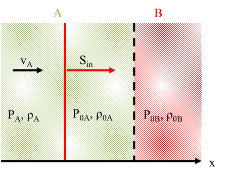
Figure E.1: Shock propagates from left to right towards density discontinuity at the boundary of materials A and B.

The shock propagates from left to right with a speed $S_{in}$. After it passes through the material A, the material acquires a velocity $v_{A}$ from left to right. Its pressure and density become $P_{A}$ and $\rho_{A}$, respectively. The quantities $v_{A}$, $P_{A}$ and $\rho_{A}$ can be found from

$$\frac{P_{A}}{P_{0}}=\frac{2\gamma M_{in}^{2}-\left(\gamma-1\right)}{\gamma+1},$$ (E.1)

$$\frac{\rho_{A}}{\rho_{0A}}=\frac{S_{in}}{S_{in}-v_{A}}=\frac{M_{in}^{2}\left(\gamma+1\right)}{M_{in}^{2}\left(\gamma-1\right)+2},$$ (E.2)

so that

$$v_{A}=\frac{2c_{0A}}{\gamma+1}\frac{M_{in}^{2}-1}{M_{in}}$$ (E.3)

where $\gamma=5/3$, $c_{0A}\equiv\sqrt{\gamma P_{0}/\rho_{0A}}$ is the upstream sound speed in the material A, and $P_{0}$, $\rho_{0A}$, and $M_{in}\equiv S_{in}/c_{0A}$ are the input parameters.

Eventually the shock $S_{in}$ arrives at the interface between the materials A and B and splits into a transmitted shock $S_{B}$, propagating through the material B from left to right; and a reflected shock (or a rarefaction wave) $S_{A}$, propagating through the material A from right to left, see Fig. E.2.

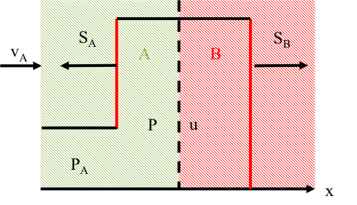
Figure E.2: After encountering the material interface, the shock $S_{in}$ splits into a transmitted shock $S_{B}$, propagating through the material B from left to right; and a reflected shock (or a rarefaction wave) $S_{A}$, propagating through the material A from right to left.

$S_{A}$ is a shock when $\rho_{0B}>\rho_{0A}$, the case considered herein; and a rarefaction wave otherwise. The material between $S_{A}$ and $S_{B}$, within the so-called contact discontinuity region, has the common pressure $P$ and flow velocity $u$ from left to right. These quantities can be evaluated by demanding downstream pressures and flow velocities for $S_{A}$ and $S_{B}$ to be equal. This is shown schematically in Fig. E.2.

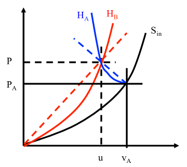
Figure E.3: Black, red, and blue lines show Hugoniot curves (in the $P-v$ variables) for shocks $S_{in}$, $S_{A}$, and $S_{B}$. The figure demonstrates graphically the process of finding material pressure and flow velocity in the contact discontinuity region. The situation depicted is only possible when the red curve is steeper than the black curve, which occurs for $\rho_{0B}>\rho_{0A}$. Then, the blue curve is as shown, corresponding to a reflected shock. When the black curve is steeper than the red one, which occurs for $\rho_{0B}<\rho_{0A}$, the reflected wave is a rarefaction wave.

The downstream flow velocity for the shock $S_{B}$ is given as:

$$(S_{B}-u)^{2}=\frac{c_{0B}^{2}}{2\gamma}\frac{\left[(\gamma+1)+(\gamma-1)P/P_{0}\right]^{2}}{(\gamma-1)+(\gamma+1)P/P_{0}}$$ (E.4)

with $c_{0B}\equiv\sqrt{\gamma P_{0}/\rho_{0B}}$. The shock velocity, $S_{B}$, is obtained from

$$\frac{S_{B}}{S_{B}-u}=\frac{(\gamma-1)P_{0}+(\gamma+1)P}{(\gamma+1)P_{0}+(\gamma-1)P},$$ (E.5)

resulting in

$$\frac{S_{B}}{u}=\frac{(\gamma-1)+(\gamma+1)P/P_{0}}{2(P/P_{0}-1)}.$$ (E.6)

Combining these two results gives

$$u^{2}=\frac{2c_{0B}^{2}}{\gamma}\frac{(P/P_{0}-1)^{2}}{(\gamma-1)+(\gamma+1)P/P_{0}}.$$ (E.7)

In the limit of a strong shock $S_{B}$, $P/P_{0}\gg 1$, this becomes

$$u^{2}\approx\frac{2P}{(\gamma+1)\rho_{0B}},\,\,\,\frac{S_{B}}{u}\approx\frac{\gamma+1}{2}.$$ (E.8)

Downstream flow velocity for the shock $S_{A}$ is found similarly:

$$(S_{A}+u)^{2}=\frac{c_{A}^{2}}{2\gamma}\frac{\left[(\gamma+1)+(\gamma-1)P/P_{A}\right]^{2}}{(\gamma-1)+(\gamma+1)P/P_{A}}$$ (E.9)

with $c_{A}\equiv\sqrt{\gamma P_{A}/\rho_{A}}$. The shock velocity $S_{A}$ is obtained from

$$\frac{S_{A}+v_{A}}{S_{A}+u}=\frac{(\gamma-1)P_{A}+(\gamma+1)P}{(\gamma+1)P_{A}+(\gamma-1)P},$$ (E.10)

resulting in

$$S_{A}=\frac{(\gamma-1)(Pv_{A}-P_{A}u)+(\gamma+1)(P_{A}v_{A}-Pu)}{2(P-P_{A})}.$$ (E.11)

Combining these two results gives

$$(v_{A}-u)^{2}=\frac{2c_{A}^{2}}{\gamma}\frac{(P/P_{A}-1)^{2}}{(\gamma-1)+(\gamma+1)P/P_{A}}.$$ (E.12)

While the transmitted shock can be strong, $P/P_{0}\text{$\gg$1}$, the reflected one does not have to be so since $P/P_{A}=(P/P_{0})(P_{0}/P_{A})\sim M_{in}^{-2}(P/P_{0})$. Thus, we should not expand Eq. (E.12) in $P/P_{A}\gg 1$.

Equating $u$ from Eqs. (E.8) and (E.12) and assuming $M_{in}\gg 1$ gives the following equation for $x\equiv\sqrt{P/P_{A}}$:

$$\sqrt{\frac{\rho_{0A}}{\rho_{0B}}}x+\frac{x^{2}-1}{\sqrt{1+\frac{\gamma+1}{\gamma-1}x^{2}}}=1.$$ (E.13)

The solution for $\gamma=5/3$ is shown in Fig. E.4 and confirms that $P/P_{A}\sim\text{O}\left(1\right)$. In general, we have to solve a combination of Eqs. (E.7) and (E.12) numerically without assuming $P/P_{0}\gg 1$, $M_{in}\gg 1$. Once $P/P_{A}$ is evaluated, all the other quantities can be obtained from the preceding equations. E.g.,

$$\frac{u}{c_{0B}}\approx\sqrt{\frac{2}{\gamma(\gamma+1)}\frac{P}{P_{0}}}\approx\frac{2}{\gamma+1}M_{in}\sqrt{\frac{P}{P_{A}}}.$$ (E.14)

Figure E.4: Solution of Eq. (E.13) for $\gamma=5/3$.

The transmitted shock has a Mach number

$$M_{B}\equiv\frac{S_{B}}{c_{0B}}\approx\sqrt{\frac{\gamma+1}{2\gamma}}\sqrt{\frac{P}{P_{0}}}\approx M_{in}\sqrt{\frac{P}{P_{A}}}>M_{in}.$$

At the same time, when the shock velocity is normalized to $c_{0A}$ rather than $c_{0B}$, we can see that the transmitted shock is weaker than the initial shock (see Fig. E.5):

$$M_{B}^{\prime}\equiv\frac{S_{B}}{c_{0A}}\approx M_{in}\sqrt{\frac{P}{P_{A}}\frac{\rho_{0A}}{\rho_{0B}}}<M_{in}.$$

Finally, the reflected shock speed is given by (E.11),

$$\frac{S_{A}}{v_{A}}=\frac{(\gamma-1)\left(\frac{P}{P_{A}}-\frac{u}{v_{A}}\right)+(\gamma+1)\left(1-\frac{P}{P_{A}}\frac{u}{v_{A}}\right)}{2\left(\frac{P}{P_{A}}-1\right)}$$

with

$$\frac{u}{v_{A}}\approx\sqrt{\frac{\rho_{0A}}{\rho_{0B}}\frac{P}{P_{A}}}<1$$ (E.15)

or, alternatively,

$$M_{A}\equiv\frac{S_{A}}{c_{A}}\approx\sqrt{\frac{2}{\gamma(\gamma-1)}}\frac{S_{A}}{v_{A}}.$$

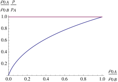
Figure E.5: The factor $(p/p_{A})(\rho_{0A}/\rho_{0B})$ for $\gamma=5/3$.

The shocked material densities are evaluated in the usual fashion:

$$\frac{\rho_{B}}{\rho_{0B}}=\frac{S_{B}}{S_{B}-u}\approx\frac{\gamma+1}{\gamma-1},\frac{\rho_{A}^{\prime}}{\rho_{A}}=\frac{S_{A}+v_{A}}{S_{A}+u}=\frac{(\gamma+1)\frac{P}{P_{A}}+(\gamma-1)}{(\gamma-1)\frac{P}{P_{A}}+(\gamma+1)}>1,$$

where $\rho_{A}^{\prime}$ is the material A density after passage of the reflected shock $S_{A}$.

Appendix F Discrete momentum conservation proof for the Vlasov equation

Expanding Eqs. (3.41), (3.42), (3.43), and discretely summing over configuration space, we obtain:

$$\int_{L_{min}}^{L_{max}}dx\left\{v^{*}\partial_{x}\left(v^{*}\widehat{S}_{2,||}\right)\right\}-\left\{\partial_{x}\left[\left(v^{*}\right)^{2}\widehat{S}_{2,||}\right]-\partial_{x}v^{*}\left[v^{*}\widehat{S}_{2,||}\right]\right\}\approx$$

$$\sum_{i}^{N_{x}}v_{i}^{*}\left(v_{i+1/2}^{*}\widehat{S}_{2,||,i+1/2}-v_{i-1/2}^{*}\widehat{S}_{2,||,i-1/2}\right)-\sum_{i}^{N_{x}}\left(\left(v_{i+1/2}^{*}\right)^{2}\widehat{S}_{2,||,i+1/2}-\left(v_{i-1/2}^{*}\right)^{2}\widehat{S}_{2,||,i-1/2}\right)+$$

$$\frac{1}{2}\sum_{i}^{N_{x}}\left\{\left(v_{i+1}^{*}-v_{i}^{*}\right)v_{i+1/2}^{*}\widehat{S}_{2,||,i+1/2}+\left(v_{i}^{*}-v_{i-1}^{*}\right)v_{i-1/2}^{*}\widehat{S}_{2,||,i-1/2}\right\}.$$ (F.1)

With periodic boundary conditions, the second summation vanishes. Gathering terms, we find:

$$\sum_{i}^{N_{x}}v_{i}^{*}\left(v_{i+1/2}^{*}\widehat{S}_{2,||,i+1/2}-v_{i-1/2}^{*}\widehat{S}_{2,||,i-1/2}\right)$$

$$+\frac{1}{2}\sum_{i}^{N_{x}}\left\{\left(v_{i+1}^{*}-v_{i}^{*}\right)v_{i+1/2}^{*}\widehat{S}_{2,||,i+1/2}+\left(v_{i}^{*}-v_{i-1}^{*}\right)v_{i-1/2}^{*}\widehat{S}_{2,||,i-1/2}\right\} =$$ (F.2)

$$\sum_{i}^{N_{x}}\left(v_{i+1/2}^{*}\right)^{2}\widehat{S}_{2,||,i+1/2}-\sum_{i}^{N_{x}}\left(v_{i-1/2}^{*}\right)^{2}\widehat{S}_{2,||,i-1/2} = 0.$$ (F.3)

Appendix G Discrete energy conservation proof for the Vlasov equation

Expanding Eqs. (3.48), (3.49), (3.50), and discretely summing over configuration space, we obtain:

$$\int_{L_{min}}^{L_{max}}dx\left\{\left(v^{*}\right)^{2}\partial_{x}\left(v^{*}\widehat{S}_{3,||}\right)\right\}-\left\{\partial_{x}\left[\left(v^{*}\right)^{3}\widehat{S}_{3,||}\right]-\partial_{x}\left(v^{*}\right)^{2}\left[v^{*}\widehat{S}_{3,||}\right]\right\}\approx$$

$$\sum_{i}^{N_{x}}\left(v_{i}^{*}\right)^{2}\left(v_{i+1/2}^{*}\widehat{S}_{3,||,i+1/2}-v_{i-1/2}^{*}\widehat{S}_{3,||,i-1/2}\right)-\sum_{i}^{N_{x}}\left(\left(v_{i+1/2}^{*}\right)^{3}\widehat{S}_{3,||,i+1/2}-\left(v_{i-1/2}^{*}\right)^{3}\widehat{S}_{3,||,i-1/2}\right)+$$

$$\frac{1}{2}\sum_{i}^{N_{x}}\left\{\left(\left[\left(v_{i+1}^{*}\right)^{2}-\left(v_{i}^{*}\right)^{2}\right]\right)v_{i+1/2}^{*}\widehat{S}_{3,||,i+1/2}+\left[\left(v_{i}^{*}\right)^{2}-\left(v_{i-1}^{*}\right)^{2}\right]v_{i-1/2}^{*}\widehat{S}_{3,||,i-1/2}\right\}.$$ (G.1)

With periodic boundary conditions, the second summation vanishes. Gathering terms, we find:

$$\sum_{i}^{N_{x}}\left(v_{i}^{*}\right)^{2}\left(v_{i+1/2}^{*}\widehat{S}_{3,||,i+1/2}-v_{i-1/2}^{*}\widehat{S}_{3,||,i-1/2}\right)$$

$$+\frac{1}{2}\sum_{i}^{N_{x}}\left\{\left[\left(v_{i+1}^{*}\right)^{2}-\left(v_{i}^{*}\right)^{2}\right]v_{i+1/2}^{*}\widehat{S}_{3,||,i+1/2}+\left[\left(v_{i}^{*}\right)^{2}-\left(v_{i-1}^{*}\right)^{2}\right]v_{i-1/2}^{*}\widehat{S}_{3,||,i-1/2}\right\} =$$ (G.2)

$$\sum_{i}^{N_{x}}\left[\left(v_{i}^{*}\right)^{2}+\left(v_{i+1}^{*}\right)^{2}\right]v_{i+1/2}^{*}\widehat{S}_{3,||,i+1/2}-\sum_{i}\left[\left(v_{i-1}^{*}\right)^{2}+\left(v_{i}^{*}\right)^{2}\right]v_{i-1/2}^{*}\widehat{S}_{3,||,i-1/2} = 0.$$ (G.3)

References

- [1] M. N. Rosenbluth, W. M. Macdonald, and D. L. Judd, “Fokker-Planck equation for an inverse-square force,” Phys. Rev., vol. 107, no. 1, pp. 1–6, 1957.
- [2] A. A. Arsen’ev and O. E. Buryac, “On the connection between a solution of the Boltzmann equation and a solution of the Landau-Fokker-Planck equation,” USSR Comput. Maths math. Phys., vol. 17, pp. 241–246, 1991.
- [3] L. Desvillettes, “On asymptotics of the Boltzmann equation when the collisions become grazing,” Trans. Theory and Stat. Phys., vol. 21, no. 3, pp. 259–276, 1992.
- [4] P. Degond and B. Lucquin-Desreux, “The Fokker-Planck asymptotics of the Boltzmann collision operator in the Coulomb case,” Math. Models Meth. Appl. Sci., vol. 2, no. 2, pp. 167–182, 1992.
- [5] T. Goudon, “On Boltzmann equations and Fokker-Planck asymptotics: Influence of grazing collisions,” J. Stat. Phys., vol. 89, no. 3/4, pp. 751–776, 1997.
- [6] L. D. Landau, “The kinetic equation in the case of Coulomb interaction,” Phys. Zs. Sov. Union, vol. 10, pp. 154–164, 1936.
- [7] O. Larroche, “An efficient explicit numerical scheme for diffusion-type equations with a highly inhomogeneous and highly anisotropic diffusion tensor,” J. Comput. Phys., vol. 223, pp. 436–450, 2007.
- [8] O. Larroche, “Kinetic simulations of fuel ion transport in ICF target implosions,” Eur. Phys. J. D, vol. 27, pp. 131–146, 2003.
- [9] D. Jarema, H. J. Bungartz, T. Görler, F. Jenko, T. Neckel, and D. Told, “Block-structured grids for eulerian gyro kinetic simulations,” Comput. Phys. Commun., vol. 198, pp. 105–117, 2016.
- [10] B. E. Peigney, O. Larroche, and V. Tikhonchuk, “Fokker-Planck kinetic modeling of supra thermal -particles in a fusion plasma,” J. Comput. Phys., vol. 278, pp. 416–444, 2014.
- [11] O. Larroche, “Ion Fokker-Planck simulation of D-3He gas target implosions,” Phys. Plasmas, vol. 19, p. 122706, 2012.
- [12] A. Inglebert, B. Canaud, and O. Larroche, “Species separation and modification of neutron diagnostics in inertial-confinement fusion,” Euro. Phys. Lett., vol. 107, p. 65003, 2014.
- [13] W. T. Taitano, L. Chacón, and A. N. Simakov, “An adaptive, conservative 0D-2V multispecies Rosenbluth-Fokker-Planck solver for arbitrarily disparate mass and temperature regimes,” J. Comput. Phys., vol. 318, pp. 391–420, 2016.
- [14] W. T. Taitano, L. Chacón, A. N. Simakov, and K. Molvig, “A mass, momentum, and energy conserving, fully implicit, scalable algorithm for the multi-dimensional, multi-species Rosenbluth-Fokker-Planck equation,” J. Comput. Phys., vol. 297, pp. 357–380, 2015.
- [15] S. I. Braginskii, “Transport processes in a plasma,” in Reviews of Plasma Physics (M. A. Leontovich, ed.), vol. 1, pp. 205–311, New York: Consultants Bureau, 1965.
- [16] A. N. Simakov and K. Molvig, “Electron transport in a collisional plasma with multiple ion species,” Phys. Plasmas, vol. 21, p. 024503, 2014.
- [17] R. D. Hazeltine and J. D. Meiss, Plasma Confinement. Redwood City, CA: Addison-Wesly Publishing Company, 1991.
- [18] R. D. Hazeltine, Plasma confinement. Addison-Wesley, 1992.
- [19] P. H. Gaskell and A. K. C. Lau, “Curvature-compensated convective transport: SMART, a new boundedness-preserving transport algorithm,” International Journal for Numerical Methods in Fluids, vol. 8, pp. 617–641, 1988.
- [20] K. Lipnikov, D. Svyatskiy, and Y. Vassilevski, “Minimial stencil finite volume scheme with the discrete maximum principle,” Russ. J. Numer. Anal. Math. Modelling, vol. 27, no. 4, pp. 369–385, 2012.
- [21] M. Casanova, O. Larroche, and J. Matte, “Kinetic simulation of a collisional shock wave in a plasma,” Phys. Rev., vol. 67, no. 16, pp. 2143–2146, 1991.
- [22] W. T. Taitano, L. Chacón, and A. N. Simakov, “An equilibrium-preserving discretization for the nonlinear Fokker-Planck operator in arbitrary multi-dimensional geometry,” J. Comput. Phys., vol. 339, pp. 453–460, 2017.
- [23] D. G. Anderson, “Iterative procedures for nonlinear integral equations,” J. Assoc. Comput. Mach., vol. 12, pp. 547 – 560, 1965.
- [24] M. Gasteiger, L. Einkemmer, A. Ostermann, and D. Tskhakaya, “Alternating direction implicit type preconditioners for the steady state inhomogeneous Vlasov equation,” J. Plasma Physics., vol. 83, p. 705830107, 2017.
- [25] F. Vidal, J. P. Matte, M. Casanova, and O. Larroche, “Ion kinetic simulations of the formation and propagation of a planar collisional shock wave in a plasma,” Phys. Plasmas, vol. 5, p. 3182, 1993.
- [26] A. Rohatgi, “Webplotdigitizer,” 2017.
- [27] W. T. Taitano and L. Chacón, “Charge-and-energy conserving moment-based accelerator for a multi-species Vlasov-Fokker-Planck-Ampère system, part I: Collisionless aspects,” J. Comput. Phys., vol. 284, pp. 718–736, 2015.