Inverse Ising problem in continuous time: A latent variable approach

Abstract

We consider the inverse Ising problem, i.e. the inference of network couplings from observed spin trajectories for a model with continuous time Glauber dynamics. By introducing two sets of auxiliary latent random variables we render the likelihood into a form, which allows for simple iterative inference algorithms with analytical updates. The variables are: (1) Poisson variables to linearise an exponential term which is typical for point process likelihoods and (2) Pólya–Gamma variables, which make the likelihood quadratic in the coupling parameters. Using the augmented likelihood, we derive an expectation–maximization (EM) algorithm to obtain the maximum likelihood estimate of network parameters. Using a third set of latent variables we extend the EM algorithm to sparse couplings via L1 regularization. Finally, we develop an efficient approximate Bayesian inference algorithm using a variational approach. We demonstrate the performance of our algorithms on data simulated from an Ising model. For data which are simulated from a more biologically plausible network with spiking neurons, we show that the Ising model captures well the low order statistics of the data and how the Ising couplings are related to the underlying synaptic structure of the simulated network.

I Introduction

In recent years, the inverse Ising problem, i.e. the reconstruction of couplings and external fields of an Ising model from samples of spin configurations, has attracted considerable interest in the physics community Nguyen et al. (2017). This is due to the fact that Ising models play an important role for data modeling with applications to neural spike data Schneidman et al. (2006); Roudi et al. (2009), protein structure determination Weigt et al. (2009), and gene expression analysis Lezon et al. (2006). Much effort has been devoted to the development of algorithms for the static inverse Ising problem. This is a nontrivial task, because statistically efficient, likelihood based methods become computationally infeasible by the intractability of the partition function of the model. Hence one has to resort to either approximate inference methods or to other statistical estimators such as pseudo–likelihood methods Bachschmid-Romano and Opper (2017), or the interaction screening algorithm Vuffray et al. (2016). The situation is somewhat simpler for the dynamical inverse Ising problem, which recently attracted attention Roudi and Hertz (2011a); Mézard and Sakellariou (2011); Roudi and Hertz (2011b); Zeng et al. (2011); Tyrcha et al. (2013); Keshri et al. (2013). If one assumes a Markovian dynamics, the exact normalisation of the spin transition probabilities allows for an explicit computation of the likelihood if one has a complete set of observed data over time. Nevertheless, the model parameters enter the likelihood in a fairly complex way, and the application of more advanced statistical approaches such as Bayesian inference again becomes a nontrivial task. This is especially true for the continuous time kinetic Ising model where the spins are governed by Glauber dynamics Glauber (1963). With this dynamics the likelihood contains an exponential function related to the ’non–flipping’ times and makes analytical manipulations of the posterior distribution of parameters intractable. However, it is possible to compute the likelihood gradient to find the maximum likelihood estimate (MLE) Zeng et al. (2013).

In this paper we will show how the likelihood for the continuous time problem can be remarkably simplified by introducing a combination of two sets of auxiliary random variables. The first set of variables are Poisson random variables which ’linearise’ the aforementioned exponential term that appears naturally in likelihoods of Poisson point–process models Wilkinson (2006). These latent variables are related to previous work, where similar variables have been introduced for sampling the intensity function of an inhomogeneous Poisson process Adams et al. (2009). The second set of variables are the so–called Pólya–Gamma variables, which were introduced into statistics to enable efficient Bayesian inference for logistic regression Polson et al. (2013) and which may not be familiar in the physics community. These variables have also been used recently for Monte Carlo based Bayesian inference of discrete-time Markov modelsLinderman et al. (2015), model based statistical testing of spike synchrony Scott et al. (2015), and an expectation–maximization (EM) scheme for logistic regression Scott and Sun (2013).

With these latent variables the model parameters enter the resulting joint likelihood similarly to simple Gaussian models. We will use this formulation to construct iterative algorithms for a penalised maximum likelihood and for variational Bayes estimators which have simple analytically computable updates. We test our algorithms on artificial data. As an illustrative application we use the Bayes algorithm on data from a simulated recurrent network with conductance–based spiking neurons and show how the model reproduces the statistics of the data and how the obtained Ising parameters reflect the underlying synaptic structure.

The paper is organized as follows: In Sec. II the continuous time kinetic Ising model is introduced followed by a derivation of its likelihood in Sec. III. In Sec. IV we introduce auxiliary latent variables to simplify the likelihood. In Sec. V we develop an EM algorithm for maximum likelihood inference and extend it to L1–regularized likelihood maximisation and a variational Bayes approximation. Finally, in Sec. VI we apply our method to simulated data generated from an Ising network and from a network of spiking neurons.

II The Model

Following Ref. Zeng et al. (2013) in this section, we consider a system of $N$ Ising spins $s_{i}(t)\in\{-1,1\}$ for $i=1,\ldots,N$. We denote the vector of all spins by $\bm{s}(t)=(s_{1}(t),\ldots,s_{N}(t))^{\top}$. A spin $i$ is interacting with spin $j$ through a coupling $J_{ij}$. We are not assuming symmetry of these couplings: in general, we have $J_{ij}\neq J_{ji}$. We will also allow for self couplings $J_{ii}$. The total field acting on spin $i$ is given by

$$H_{i}(t)=\theta_{i}+\sum_{j=1}^{N}J_{ij}s_{j}(t),$$ (1)

where $\theta_{i}$ denotes the external field. The Glauber dynamics of the spins is defined by asynchronous updates Zeng et al. (2013) where in a small time interval $\Delta t$, spins $i$ are selected independently with probability $\gamma\Delta t$ for an update; $\gamma>0$ is the update rate. The updated spins are flipped, i.e., $s_{i}(t+\Delta t)=-s_{i}(t)$ with probability

$$P_{i}^{\text{\small{flip}}}(t)=\frac{\exp(-s_{i}(t)H_{i}(t))}{2\cosh(H_{i}(t))}.$$ (2)

The probability that spin $i$ is not flipped at time $t$ in the interval $\Delta t$ is given by $1-\gamma\Delta t+\gamma\Delta t\left(1-P_{i}^{\text{\small{flip}}}(t)\right).$ Hence, the total probability of a (time–discretised) temporal sequence $\{\bm{s}\}_{0:T}$ of spins during a time interval $[0:T]$ is given by

$$\begin{split}&P(\{\bm{s}\}_{0:T}|\bm{J})=\prod_{(i,t)\in F}\left\{\gamma\Delta t\frac{\exp(-s_{i}(t)H_{i}(t))}{2\cosh(H_{i}(t))}\right\}\\ &\times\prod_{(i,t)\in NF}\left\{1-\gamma\Delta t+\gamma\Delta t\frac{\exp(s_{i}(t)H_{i}(t))}{2\cosh(H_{i}(t))}\right\}.\end{split}$$ (3)

Here $F$ denotes the set of pairs $(i,t)$ where spin $i$ was flipped at time $t$. and $NF$ is the corresponding, complementary set of times and spins where no flips happened. $\bm{J}$ stands for the parameters of the model: $\bm{J}\equiv J_{ij}$ for $i,j=1,\ldots N$ and $\theta_{i}$ for $i=1,\ldots,N$.

III Likelihood and Inference

Our goal is to infer the couplings and external fields from observations of complete spin trajectories over a time interval $[0,T]$. We will consider only likelihood based approaches in this paper. Hence, we need to compute the probability of spin trajectories (3) as a function of parameters, i.e., the so–called likelihood function in continuous time. Taking the limit $\Delta t\to 0$ in (3) and discarding prefactors which contain $\Delta t$ but are irrelevant for inference (being independent of $\bm{J}$), the complete–data likelihood function Wilkinson (2006) is found to be

$$\begin{split}&{\cal{L}}(\{\bm{s}\}_{0:T}|\bm{J})=\prod_{(i,t)\in F}\frac{\exp(-s_{i}(t)H_{i}(t))}{2\cosh(H_{i}(t))}\\ &\times\prod_{i=1}^{N}\exp\left(\gamma\int_{0}^{T}\left\{\frac{\exp(s_{i}(t)H_{i}(t))}{2\cosh(H_{i}(t))}-1\right\}dt\right).\end{split}$$ (4)

A maximum likelihood estimate of the parameters $\bm{J}$ can be obtained by a (possibly penalised) gradient ascent approach of this function Zeng et al. (2013). However, a Bayesian inference approach does not seem to be feasible from the expression (4). For a Bayesian approach one would introduce a prior density $p(\bm{J})$ of parameters and would infer statistical properties of $\bm{J}$ using the posterior density given by

$$p(\bm{J}|\{\bm{s}\}_{0:T})=\frac{{\cal{L}}(\{\bm{s}\}_{0:T}|\bm{J})p(\bm{J})}{\int{\cal{L}}(\{\bm{s}\}_{0:T}|\bm{J})p(\bm{J})\;d\bm{J}},$$ (5)

from which posterior expectations of parameters would have to be calculated by high–dimensional integrals. Due to the complex dependency of the likelihood on the parameters, the application of well–known techniques such as Monte Carlo sampling, e.g. using a Gibbs sampler, or approximate inference methods such as the variational approach Bishop (2006) would not be trivial. We will show in the next section that the dependency of the likelihood on $\bm{J}$ can be remarkably simplified by augmenting the system by two sets of auxiliary random variables.

IV Variable augmentation and tractable likelihood

The two main problems that prevent us from performing efficient analytical inference using Eq. (4) come from two sources: first, the time integral which contains the parameters $\bm{J}$, appears in an exponential function, and, second, the parameters also appear in the denominators in the hyperbolic cosine function. We will show that both problems can be solved by the introduction of auxiliary variables. We will start with a simplification of the integral.

IV.1 Poisson variables

We note, that fields $H_{i}(t)$ are piecewise constant functions of time and do not change where no spin is flipped. Hence, the time integral can be calculated analytically. We will order the constant intervals and number them by $n\in\{0,1,\ldots,n_{max}\}$. We define $H_{i}^{n}$ and $s_{i}^{n}$ as the values of the field and spin $i$ between time points $t_{n}$ and $t_{n+1}$. $t_{n}$ denotes the time of the $n^{\rm{th}}$ flip time for $n\in\{1,\ldots,n_{max}\}$, while $t_{0}=0$ and $t_{n_{max}+1}=T$. Hence, we obtain

$$\int_{0}^{T}\frac{\exp(s_{i}(t)H_{i}(t))}{2\cosh(H_{i}(t))}dt=\sum_{n=0}^{n_{max}}\frac{\exp(s_{i}^{n}H_{i}^{n})}{2\cosh(H_{i}^{n})}({t_{n+1}}-{t_{n}}).$$ (6)

Introducing a set of independent Poisson distributed random variables $\rho_{i}^{n}$ for each $i$ and each time slice between $t_{n+1}$ and $t_{n}$, we obtain the following representation of the second part of the likelihood:

$$\begin{split}&\exp\left(\gamma\int_{0}^{T}\left\{\frac{\exp(s_{i}(t)H_{i}(t))}{2\cosh(H_{i}(t))}-1\right\}dt\right)\\ &=\prod_{n=0}^{n_{max}}\left\{\sum_{\rho_{i}^{n}=0}^{\infty}\left(\frac{\exp(s_{i}^{n}H_{i}^{n})}{2\cosh(H_{i}^{n})}\right)^{\rho_{i}^{n}}P_{\mathrm{Po}}\left(\rho_{i}^{n}|\gamma({t_{n+1}}-{t_{n}})\right)\right\},\end{split}$$ (7)

where

$$P_{\mathrm{Po}}(\rho|\zeta)=e^{-\zeta}\frac{\zeta^{\rho}}{\rho!},$$ (8)

denotes a Poisson distribution with mean parameter $\zeta$. For Eq. (7) we made use of the equality

$$e^{\zeta(x-1)}=\sum_{\rho=0}^{\infty}x^{\rho}P_{\mathrm{Po}}(\rho|\zeta),$$

which is the moment–generating function of the Poisson distribution Kingman (1992). Similar variables were used in Ref. Adams et al. (2009) to make Poisson–process likelihoods tractable for Monte–Carlo sampling.

IV.2 Pólya-Gamma variables

To get rid of the hyperbolic terms in the denominators, we will use a remarkable representation which was discovered and used in the statistics literature in recent years to simplify Bayesian inference for logistic regression. Reference Polson et al. (2013) found a convenient form of writing an inverse hyperbolic cosine as a continuous mixture of Gaussian densities as

$$\cosh^{-b}(x)=\int_{0}^{\infty}d\omega\ e^{-2\omega x^{2}}p_{\mathrm{PG}}(\omega|b,0),$$ (9)

where $p_{\mathrm{PG}}(\omega|b,0)$ is the Pólya-Gamma density with parameter $b$. Surprisingly, the exact form of this distribution is not of importance for our inference algorithm, but only the fact that one can derive its first moments straightforwardly (see Appendix B). Introducing Pólya-gamma variables $\omega$ into the likelihood (7) yields the representation

$$p(\{\bm{s}\}_{0:T}|\bm{J})=\sum_{\bm{\rho}}\int{\cal{L}}(\{\bm{s},\bm{\rho},\bm{\omega}\}_{0:T}|\bm{J})d\bm{\omega},$$ (10)

with the augmented likelihood

$$\begin{split}&{\cal{L}}(\{\bm{s},\bm{\rho},\bm{\omega}\}_{0:T}|\bm{J})=\\ &\prod_{(i,t)\in F}\exp\left[-s_{i}(t)H_{i}(t)-2(H_{i}(t))^{2}\omega_{i}(t)\right]p_{\mathrm{PG}}(\omega_{i}(t)|1,0)\\ &\times\prod_{i,n}\left(\exp\left[\rho_{i}^{n}(s_{i}^{n}H_{i}^{n}-\ln(2))-2(H_{i}^{n})^{2}\omega_{i}^{n}\right]\right.\\ &\left.\times P_{\mathrm{Po}}\left(\rho_{i}^{n}|\gamma({t_{n+1}}-{t_{n}})\right)p_{\mathrm{PG}}(\omega_{i}^{n}|\rho_{i}^{n},0)\right).\end{split}$$ (11)

The advantage of the augmented likelihood over the original one is the fact that the parameters appear at most quadratically in the exponential functions [note, that the fields $H_{i}(t)$ are linear functions of the parameters]. As we will see, the computation of maximum likelihood and related estimators as well as Bayesian inference become considerably facilitated. We will postpone explicit results of Gibbs sampling algorithms to a future publication and discuss applications of the augmented likelihood to penalised maximum likelihood estimation and to a variational Bayes algorithm in this paper.

V Inference

V.1 EM algorithm

The EM algorithm Dempster et al. (1977) is a convenient way to maximise the likelihood iteratively with respect to $\bm{J}$ by using latent variable representations. The algorithm cycles between an E–step and an M–step and guarantees to increase the likelihood (4) in each step. At iteration $m+1$, in the

E-step one computes the cost function $Q(\bm{J},\bm{J}_{m})$. It equals the expectation of the logarithm of the augmented likelihood with respect to the distribution of latent variables conditioned on the parameters at the previous iteration $m$

$$\begin{split}&Q(\bm{J},\bm{J}_{m})\doteq\\ &\sum_{\bm{\rho}}\int d\bm{\omega}\;p(\bm{\rho},\bm{\omega}|\{\bm{s}\}_{0:T},\bm{J}_{m})\ln{\cal{L}}(\{\bm{s},\bm{\rho},\bm{\omega}\}_{0:T}|\bm{J}).\end{split}$$ (12)

M–step Here we compute an update of the parameters via

$$\bm{J}_{m+1}=\arg\max_{\bm{J}}Q(\bm{J},\bm{J}_{m}).$$ (13)

The conditional distribution is given by

$$\begin{split}&p(\{\bm{\rho},\bm{\omega}\}_{0:T}|\{\bm{s}\}_{0:T},\bm{J})=\\ &p(\{\bm{\omega}\}_{0:T}|\{\bm{s},\bm{\rho}\}_{0:T},\bm{J})P(\{\bm{\rho}\}_{0:T}|\bm{J},\{\bm{s}\}_{0:T}),\end{split}$$ (14)

where

$$\begin{split}p(\{\bm{\omega}\}_{0:T}|\{\bm{s},\bm{\rho}\}_{0:T},\bm{J})=&\prod_{(i,t)\in F}p_{\mathrm{PG}}(\omega_{i}(t)|1,2H_{i}(t))\\ &\times\prod_{n,i}p_{\mathrm{PG}}(\omega_{i}^{n}|\rho_{i}^{n},2H_{i}^{n}),\end{split}$$ (15)

where we defined the tilted Pólya–Gamma distribution as

$$p_{\mathrm{PG}}(\omega_{i}^{n}|b,c)=\frac{\exp\left(-\frac{c^{2}}{2}\omega_{i}^{n}\right)p_{\mathrm{PG}}(\omega_{i}^{n}|b,0)}{\cosh^{-b}(c/2)},$$

and where

$$P(\bm{\rho}|\bm{J},\{\bm{s}\}_{0:T})=\prod_{n,i}P_{\mathrm{Po}}\left(\rho_{i}^{n}\left|\gamma(t_{n+1}-t_{n})\frac{\exp(s_{i}^{n}H_{i}^{n})}{2\cosh(H_{i}^{n})}\right.\right).$$ (16)

The first part of the conditional density is over factorising Pólya Gamma variables and the second one over factorising Poisson random variables. The necessary expectations for the E–step follow from simple properties of Poisson random variables and of Pólya Gamma random variables derived in Appendix B. This results in

$$\begin{split}&\langle\omega_{i}(t)\rangle=\frac{1}{4H_{i}(t)}\tanh(H_{i}(t)),\\ &\langle\omega_{i}^{n}\rangle=\frac{\langle\rho_{i}^{n}\rangle}{4H_{i}^{n}}\tanh(H_{i}^{n}),\\ &\langle\rho_{i}^{n}\rangle=(t_{n+1}-t_{n})\gamma\frac{\exp(s_{i}^{n}H_{i}^{n})}{2\cosh(H_{i}^{n})},\end{split}$$ (17)

where the brackets $\langle\cdot\rangle$ denote expectations conditioned on $\bm{J}_{m}$. Since the augmented log–likelihood is a quadratic form in the parameters $\bm{J}$, the maximisation leads to $N$ systems of linear equations for the vectors $\bm{J}_{i\cdot}\doteq(\theta_{i},J_{i1},\ldots,J_{iN})^{\top}$ of the form

$$A_{i}\bm{J}_{i\cdot}=\bm{b}_{i\cdot},$$ (18)

with

$$b_{ij}=-\sum_{t\in F(i)}s_{i}(t)s_{j}(t)+\sum_{n}\langle\rho_{i}^{n}\rangle s_{i}^{n}s_{j}^{n},$$ (19)

and

$$A_{ijk}=4\left(\sum_{t\in F(i)}\langle\omega_{i}^{t}\rangle s_{k}(t)s_{j}(t)+\sum_{n}\langle\omega_{i}^{n}\rangle s_{k}^{n}s_{j}^{n}\right).$$ (20)

Here $F(i)$ is the set of all times that spin $i$ has flipped. As mentioned before only the first moment of the Pólya–Gamma density is required.

V.2 Sparsity via L1 regularization

Assuming a factorising Laplace distribution over each coupling $J_{ij}$

$$p(J_{ij})=\frac{\lambda}{2}\exp\left(-\lambda|J_{ij}|\right),$$

will enforce sparsity on the network. $\lambda$ is the scale parameter of this density. On the level of the MAP (maximuma posteriori) Bayesian estimator this is equivalent to L1 regularised maximum likelihood estimation. However, the absolute value in the exponent of this prior would prevent us from using the previously described EM procedure directly and allow only for gradient methods similar to Ref. Zeng et al. (2014). Fortunately, this problem can again be solved by the introduction of a further auxiliary random variable for each single coupling parameter $J_{ij}$. This follows from the fact that a Laplace distribution can once more be represented as an infinite mixture of Gaussians Girosi (1991); Pontil et al. (2000),

$$\begin{split}&\frac{\lambda}{2}\exp(-\lambda|J|)=\\ &\int d\beta\sqrt{\frac{\beta\lambda^{2}}{2\pi}}\exp\left(-\frac{\beta\lambda^{2}}{2}J^{2}\right)p(\beta),\end{split}$$ (21)

with

$$p(\beta)=(\beta/2)^{-2}\exp\left(-1/(2\beta)\right).$$

By extending the augmented likelihood (11) to sparsity variables $\{\beta_{ij}\}$ a similar EM algorithm is possible to obtain the L1–regularized ML solution of $\bm{J}$. The required conditional density factorises as

$$p(\{\bm{\rho},\bm{\omega}\}_{0:T},\bm{\beta}|\{\bm{s}\}_{0:T},\bm{J})=p(\{\bm{\rho},\bm{\omega}\}_{0:T}|\{\bm{s}\}_{0:T},\bm{J})\;p(\bm{\beta}|\bm{J}),$$ (22)

where $p(\bm{\beta}|\bm{J})=\prod_{i,j}p(\beta_{ij}|J_{ij})$ and each factor is a generalized inverse Gaussian distribution

$$\begin{split}p(\beta_{ij}|J_{ij})=&p_{\mathrm{GIG}}(\beta_{ij}|a_{ij},1,\nu)\\ =&\frac{a_{ij}^{\nu/2}}{2K_{\nu}(\sqrt{a_{ij}})}\beta_{ij}^{\nu-1}\exp\left(-\frac{a_{ij}\beta_{ij}+1/\beta_{ij}}{2}\right),\end{split}$$ (23)

where $a_{ij}=\lambda^{2}J_{ij}^{2}$, $\nu=-1/2$, and $K_{\nu}$ is the modified Bessel function of the second kind. The only change in the linear system (18) is in the matrices $A$, which have to be replaced by

$$A^{sparse}_{ijk}=A_{ijk}+\delta_{i,k}\lambda^{2}\langle\beta_{ij}\rangle,$$ (24)

and where $\langle\beta_{ij}\rangle=(J_{ij}^{2}\lambda^{2})^{-1/2}$ (see Appendix C).

V.3 Approximate posterior distribution via variational Bayes

For Bayesian inference we assume the previously discussed Laplace prior over couplings $J_{ij}$ with scaling parameter $\lambda$ and for the external fields $\theta_{i}$ a Gaussian prior with mean $\mu_{\theta}$ and precision $\lambda_{\theta}^{2}$. To obtain a full posterior distribution including the couplings $\bm{J}$ we could either sample from the posterior or resort to a variational approach. The latter method is popular in the field of machine learning Bishop (2006) but has its roots in statistical physics Feynman (1998). In our case we assume approximated posterior that has the following factorising form:

$$\begin{split}&p(\bm{J},\{\bm{\omega},\bm{\rho}\}_{0:T},\bm{\beta}|\{\bm{s}\}_{0:T})\approx\\ &q(\bm{J},\{\bm{\omega},\bm{\rho}\}_{0:T},\bm{\beta})\equiv q_{1}(\bm{J})q_{2}(\{\bm{\omega},\bm{\rho}\}_{0:T},\bm{\beta}),\end{split}$$ (25)

where the two factors $q_{1}$ and $q_{2}$ are optimised to minimise the relative entropy (Kullback–Leibler) divergence:

$$\begin{split}D(q;p)=&\sum_{\bm{\rho}}\left[\int q(\bm{J},\{\bm{\omega},\bm{\rho}\}_{0:T},\bm{\beta})\right.\\ &\left.\times\ln\frac{q(\bm{J},\{\bm{\omega},\bm{\rho}\}_{0:T},\bm{\beta})}{p(\bm{J},\{\bm{\omega},\bm{\rho}\}_{0:T},\bm{\beta}|\{\bm{s}\}_{0:T})}d\bm{\omega}d\bm{\beta}d\bm{J}\right].\end{split}$$ (26)

This is equivalent to minimising the variational free energy

$$\begin{split}\mathcal{F}(q;p)=&\sum_{\bm{\rho}}\left[\int q(\bm{J},\{\bm{\omega},\bm{\rho}\}_{0:T},\bm{\beta})\right.\\ &\left.\times\ln\frac{q(\bm{J},\{\bm{\omega},\bm{\rho}\}_{0:T},\bm{\beta})}{p(\{\bm{s},\bm{\omega},\bm{\rho}\}_{0:T},\bm{J},\bm{\beta})}d\bm{\omega}d\bm{\beta}d\bm{J}\right].\end{split}$$ (27)

The negative free energy is actually a lower bound on the log marginal likelihood

$$-\mathcal{F}(q;p)\leq\int\mathcal{L}(\{\bm{s}\}_{0:T}|\bm{J})p(\bm{J})d\bm{J},$$ (28)

and can be used directly for approximate model selection Bishop (2006), while in a pure maximum likelihood approach this is not possible.

Minimising the variational free energy with respect to the factors of our factorizing distribution (25), the optimal factors turn out to be

$$q_{1}^{\star}(\bm{J})\propto\exp\left(\left\langle\ln p(\bm{J},\{\bm{s},\bm{\omega},\bm{\rho}\}_{0:T},\bm{\beta})\right\rangle_{q_{2}}\right),$$

$$q_{2}^{\star}(\{\bm{\omega},\bm{\rho}\}_{0:T},\bm{\beta})\propto\exp\left(\left\langle\ln p(\bm{J},\{\bm{s},\bm{\omega},\bm{\rho}\}_{0:T},\bm{\beta})\right\rangle_{q_{1}}\right),$$

which are obtained by iterative updates Bishop (2006). For the posterior at hand we find the optimal factor $q_{2}$ of the posterior

$$\begin{split}&q_{2}^{\star}(\bm{\rho},\bm{\omega},\bm{\beta})=\prod_{(i,t)\in F}q_{2}(\omega_{i}(t))\prod_{i,n}q_{2}(\omega_{i}^{n}|\rho_{i}^{n})q_{2}(\rho_{i}^{n})\;q_{2}(\bm{\beta})\\ =&\prod_{(i,t)\in F}p_{\mathrm{PG}}(\omega_{i}(t)|1,2\sqrt{\langle(H_{i}(t))^{2}\rangle})\\ &\times\prod_{i,n}p_{\mathrm{PG}}\left(\omega_{i}^{n}|\rho_{i}^{n},2\sqrt{\langle(H_{i}^{n})^{2}\rangle}\right)\\ &\times P_{\mathrm{Po}}\left(\rho_{i}^{n}\left|\gamma(t_{n+1}-t_{n})\frac{\exp(s_{i}^{n}\langle H_{i}^{n}\rangle)}{2\cosh\left(\sqrt{\langle(H_{i}^{n})^{2}\rangle}\right)}\right.\right)\\ &\times\prod_{(ij)}p_{\mathrm{GIG}}(\beta_{ij}|\langle J_{ij}^{2}\rangle\lambda^{2},1,-1/2).\end{split}$$ (29)

From the fact that the augmented likelihood (11) and the sparsity prior factorise in the components $\bm{J}_{i\cdot}$ it follows that the optimal posterior $q_{1}^{\star}(\bm{J})$ does so as well. Each of those factors is a Gaussian distribution with covariance and mean given by

$$\Sigma_{i}=\left(4A_{i}+\left(\tilde{\Sigma}_{i}\right)^{-1}\right)^{-1},$$ (30)

$$\bm{\mu}_{i}=\Sigma_{i}\left(b_{i}+\left(\tilde{\Sigma}_{i}\right)^{-1}\tilde{\bm{\mu}}_{i}\right),$$ (31)

where $\tilde{\Sigma}_{i}$ is a diagonal matrix with $diag(\tilde{\Sigma}_{i}^{-1})=\left(\lambda_{\theta}^{2},\lambda^{2}\left\langle\beta_{i1}\right\rangle,\ldots,\lambda^{2}\left\langle\beta_{iN}\right\rangle\right)$. The prior mean is defined as $\tilde{\bm{\mu}}_{i}=(\mu_{\theta},0,\ldots,0)^{\top}$. Similar to the EM algorithm, we have a variational step, where $q_{2}$ is optimised, given $q_{1}$ and a second one, optimising $q_{1}$ given $q_{2}$. The variational step updating $q_{2}$ differs from E–step in the sense, that here expectations over the terms with the couplings $\bm{J}$ are required and not only the pointwise estimate (see Appendix D). The variational M–step is similar to the EM algorithm, where the expectations for $A$ and $b$ are computed with respect to $q_{2}$.

The Python code of the algorithms discussed here is publicly available .

VI Results

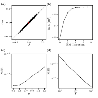
Figure 1: Inference with EM algorithm on artificial data. (a) True couplings (black dots) and external fields (red triangles) vs. inferred ones. (b) The log–likelihood as function of EM iterations. The parameters are set to $N=40$, $T=10^{3}$, and $g=0.3$ with external fields $\bm{\theta}=\bm{0}$. (c) MSE between $\bm{J}$ and $\bm{J}_{est}$ as a function of scaling factor of the variance $g$ and (d) as a function of data length $T$. If not changed parameters are as in (a).

We test the EM algorithm on artificial data generated with random couplings $J_{ij}$ from a Gaussian distribution with mean $0$ and variance $g^{2}/N$, where scaling factor $g=0.3$. With external fields $\bm{\theta}=\bm{0}$ and update rate $\gamma=100$ data is generated with a Gillespie–algorithm Wilkinson (2006) (see Appendix A).

VI.1 Maximum likelihood

In Fig. 1 the inference results for the EM algorithm are shown. Figures 1(a) and 1(b) present a single fit with $N=40$ spins and data length $T=10^{3}$. The inferred couplings $\bm{J}_{est}$ agree well with the true couplings $\bm{J}$. The logarithm of the likelihood (4) converges well after eight EM iterations. The mean squared error (MSE) increases with increasing scaling of the coupling variance $g$ [Fig. 1 (c)] and decreases linearly on a log-log scale with increasing data length $T$ [Fig. 1 (d)].

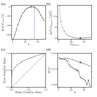
Figure 2: Inference of sparse couplings with EM and variational Bayes. Artificial data ($T=50,N=25,g=0.3$) are generated, but each coupling is set to $0$ with probability $p_{\mathrm{sparse}}=1/2$. (a) Difference in likelihood (with respect to the likelihood obtained with optimal $\lambda^{\star}$) of couplings $\bm{J}_{est}$ inferred by EM as a function of regularization parameter $\lambda$. Likelihood $\mathcal{L}_{\rm{test}}$ is computed on unseen test data ($T=50$). The optimal parameter is $\lambda^{\star}=29.4$ (red diamond). The vertical line marks the variational estimation $\lambda^{\star}_{Bayes}$. (b) Difference in free energy $\mathcal{F}$ (with respect to the likelihood obtained with estimate of optimal $\lambda^{\star}_{Bayes}$) of the variational Bayes algorithm. The optimal parameter is $\lambda_{Bayes}^{\star}=34.5$ (blue diamond). (c) ROC curves for the $\lambda^{\star}$ (EM, solid red line) and $\lambda_{Bayes}^{\star}$ (Bayes, dashed blue line), respectively. (d) The AUC for different parameters $\lambda$ for the EM result (solid black line with squares) and the variational Bayes algorithm (dashed gray line with triangles). Diamonds mark the optimal $\lambda^{\star}$ and the estimate $\lambda^{\star}_{Bayes}$.

VI.2 L1 Regularization and Variational Bayes

Regularization becomes particular important once little data are at hand. To test this we generate couplings as before for a network of $N=25$ spins, but a coupling is set to $0$ with probability of $p_{\mathrm{sparse}}=0.5$. Generated data have length $T=50$. We run the L1–regularized EM algorithm with different values of $\lambda$ and define the optimal $\lambda^{\star}$, whose MLE $\bm{J}_{est}$ maximises the likelihood $\mathcal{L}_{\rm{test}}$ on unseen test data ($T=50$) generated by the true Ising parameters $\bm{J}$ [see Fig. 2 (a)]. For inference by the variational algorithm on the same training data we estimate the optimal $\lambda^{\star}_{Bayes}$ by taking the value that minimises the free energy (27) [Fig. 2 (b)]. Note, that the Bayesian algorithm requires no test data for this estimate.

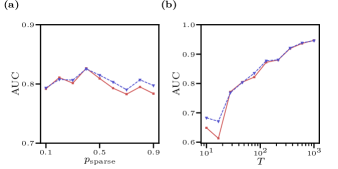
Figure 3: The classification of non–zero couplings depending on sparsity of couplings and data length. (a) The AUC depending on the sparsity, i.e. the probability of a true coupling being $0$, and in (b) depending on length of training data $T$. Results for EM shown by the red solid and variational Bayes algorithm by the blue dashed line. If not changed, parameters are as in Fig.  2.

Next we try to find the nonzero couplings from our fitting results. For the L1–penalized MLE an estimated coupling is considered as nonzero if $|J_{ij}^{est}|\geq z$, where the $z$ is an arbitrary threshold. To make use of the additional information of uncertainty, for the variational Bayes couplings are considered to be nonzero if $|\langle J_{ij}\rangle_{q_{1}}|\geq z\sqrt{(\Sigma_{i})_{(jj)}}$. The classification of nonzero-couplings is quantified by plotting the false positive rate (proportion of zero couplings that are misclassified as nonzero) versus the true positive rate (proportion of nonzero couplings that are correctly classified as nonzero) for a varying threshold $z\in[0,\infty]$. This is the Receiver–Operator characteristic (ROC) curve (see Fig. 2 (c) for $\lambda^{\star}$ and $\lambda_{Bayes}^{\star}$ respectively). As a measure of classification performance we use the area under the ROC curve (AUC), which is $1$ for perfect classification and $1/2$ at chance level. Figure 2(d) shows that performance for the EM and the variational Bayes algorithm differ only marginally. For both algorithms the AUC is approximately constant, when repeating the same data generating and fitting procedure as before, but with varying sparsity $p_{\rm{sparse}}$ [Fig. 3 (a)]. When increasing the length of training data $T$ the AUC increases as expected [Fig. 3 (b)]. For subsequent analysis we will focus on the variational Bayes algorithm.

VI.3 Inference of biophysical network

As an application of our algorithm we fit our model to data generated from a more biologically plausible network. We simulate a recurrent network of $1000$ leaky integrate–and–fire neurons ($800$ excitatory and $200$ inhibitory neurons) receiving Poisson input (see Appendix E and Ref. Renart et al. (2010)). The synapses connect neurons randomly, are conductance–based, and vary in strengths and delays. The network is simulated for $T=1000\rm{s}$. Spike times of $30$ excitatory and $10$ inhibitory neurons are used for fitting the kinetic Ising model, where neuron $i$ is considered as ’active’ for $10\rm{ms}(=\gamma^{-1})$ after each spike $s_{i}(t)=1$ and ’inactive’ otherwise [$s_{i}(t)=-1$]. The two questions we address here are, (1) how well does the fitted model reproduce the statistics of the recorded data, and (2) how are the synapses reflected in the estimated coupling parameters $\bm{J}$?

For the first question we compare data obtained from the spiking network with data sampled from the fitted the kinetic Ising model $\langle\bm{J}\rangle_{q_{1}}$ $(T=1000\rm{s})$. To compare the original data with the Ising model data the (second–order) correlations from these data are computed as

$$C_{ij}=\frac{1}{T}\int_{0}^{T}(s_{i}(t)-m_{i})(s_{j}(t)-m_{j})dt,$$ (32)

where the mean is given by $m_{i}=\int_{0}^{T}s_{i}(t)dt/T$.

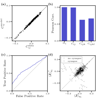
Figure 4: Model fitted to data from a simulated recurrent network. (a) Second–order correlation $C_{ij}$ of the original data vs. data sampled from mean couplings $\langle\bm{J}\rangle_{q_{1}}$ obtained via variational Bayes. (b) Pearson correlation between first to fourth order correlations of real sampled data. (c) ROC curve for identifying synapses with posterior over couplings $\bm{J}$ ($\rm{AUC}=0.65,\lambda^{\star}_{Bayes}=16.5$). (d) Mean couplings $\langle\bm{J}\rangle_{q_{1}}$ of the variational posterior vs. transpose. Couplings between neurons connected by a synapse are marked with gray triangles.

The results are compared in Fig. 4(a), and we find good agreement of original data and Ising samples. Furthermore, we compute the higher order correlations $C_{ijk}$ and $C_{ijkl}$ of the data and calculate the Pearson correlation coefficient between correlations from the original and the sampled data [see Fig. 4(b)]. The first two correlations ($m_{i}$ and $C_{ij}$) yield a Pearson correlation close to $1$. Interestingly the Pearson correlation coefficient is strongly positive for $C_{ijk}$ and $C_{ijkl}$ as well, indicating that the Ising model also carries information about higher order correlations in the data.

As before we try to identify synapses in the simulated network by ROC curve analysis (Fig. 4 (c)). The classification yields an $\rm{AUC}=0.65$ ($\lambda^{\star}_{Bayes}=16.5$). Even though there is information about the synapses, many more nonzero couplings are estimated that do not directly reflect synapses in the network. This is possibly caused by the fact, that the network is only partially observed and the kinetic Ising model compensates for this part with more nonzero couplings.

Previous work has indicated for the kinetic Ising model in discrete time Hertz et al. (2011); Zeng et al. (2013), that for experimental data recorded in vivo the estimated couplings $\bm{J}$ show a symmetric signature: $J_{ij}\approx J_{ji}$. This is particularly interesting for the Ising model in continuous time, since for the model with symmetric couplings the stationary distribution is given by the maximum entropy equilibrium model Glauber (1963) and potentially justifies the use of static Ising models for such data. As an indicator for symmetry we plot the mean of the variational posterior obtained from the recurrent network versus its transpose [Fig. 4 (d)]. We observe, that many couplings are indeed close to the diagonal, while some show large deviations from it. However, those with strong deviations correspond to the couplings which reflect synapses in the underlying network. Hence, the approximately symmetric part is not caused by synapses, but either by our data transformation to fit the Ising model or by the fact that we only partially observe the network.

VII Discussion

In this paper we have presented efficient algorithms for inferring the couplings of a continuous time kinetic Ising model defined by Glauber dynamics. Using a combination of two auxiliary latent variable sets the complete data log–likelihood becomes a simple quadratic function in the couplings. A third set of auxiliary variables allows us to deal with sparse couplings, equivalent to an L1–penalized likelihood without resorting to gradient–based algorithms Zeng et al. (2014). Using this representation we derive an EM algorithm for (penalised) maximum likelihood estimation of the couplings with explicit analytical updates. This leads to a guaranteed increase of the likelihood in each iteration. The computational complexity is similar to a Newton–Raphson method for optimising the original log–likelihood, since the Hessian matrix requires a similar inverse of the summed data covariances Zeng et al. (2013). However, our algorithm does not require any tuning of a step size.

We have extended our latent variable approach to a Bayesian scenario but have restricted ourselves to a fast variational Bayes approximation. However, it is straightforward to develop a Monte Carlo Gibbs sampler for the latent variable structure. This would require drawing samples from Pólya–Gamma density rather than computing only its mean. We have tested our inference algorithms on simulated data demonstrating fast convergence of the method. The variational Bayes approximation allows us to perform model selection, yielding hyper–parameters which achieve close to optimal likelihoods on test data. As an application of our approach we have investigated the quality of the kinetic Ising model to describe data which were generated from a more realistic, biologically inspired integrate and fire neural network model which is only partially observed. We have shown that the kinetic Ising model reproduces low order statistics of the data well. However, the partial observation of neurons prohibits a safe identification of synapses in terms of the Ising coupling parameters. It would be interesting to see if the performance of a kinetic Ising model on such data could be improved by including explicit unobserved neurons and their couplings in the model Roudi and Taylor (2015). We expect that our latent variable approach would facilitate statistical inference for such an extended model and provide alternatives to current approximate inference methods Tyrcha and Hertz (2013); Dunn and Roudi (2013); Bachschmid-Romano and Opper (2014); Battistin et al. (2015). We are currently working on an extension of our inference approach by including time–dependent model parameters which makes the model more realistic and which has been shown of importance for biological data analysis Tyrcha et al. (2013); Donner et al. (2017).

Finally, our latent variable approach should also be applicable to other inference problems for point process models; e.g., a combination with Gaussian process priors should allow for nonparametric approximate inference of rate functions for inhomogeneous Poisson processes Adams et al. (2009). Models with similar point–process likelihoods are common in neuroscience Brillinger (1988); Paninski (2004); Latimer et al. (2014), for modeling seismic activity Ogata (1998), analyzing social network analysis Zhao et al. (2015), etc.

VIII Acknowledgements

C.D. was supported by the Deutsche Forschungsgemeinschaft (GRK1589/2).

Appendix A Generating Data

To generate artificial data for the kinetic Ising model in continuous time we can make use of the Gillespie algorithm Wilkinson (2006). Having a coupling matrix $\bm{J}$ for $N$ spins and an initial data vector $\bm{s}(0)$ data are generated as follows: (1) We draw the next update time $t^{\prime}$ from a exponential distribution with mean $(\gamma\times N)^{-1}$, (2) we draw a spin $i$ with probability $1/N$, and finally (3) we flip spin $i$ at time $t^{\prime}$ according to Eq. (2) and set $t\leftarrow t^{\prime}$. These three steps are repeated until $t\geq T$.

Appendix B Properties of Pólya–Gamma distribution

The Pólya–Gamma density Polson et al. (2013) allows us to represent the inverse hyperbolic cosine function as an infinite Gaussian mixture

$$\cosh^{-b}(c/2)=\int_{0}^{\infty}d\omega\exp(-\frac{c^{2}}{2}\omega)p_{\mathrm{PG}}(\omega|b,0).$$ (33)

Furthermore, we define the tilted Pólya–Gamma distribution as

$$p_{\mathrm{PG}}(\omega|b,c)\propto e^{-c^{2}/2\omega}p_{\mathrm{PG}}(\omega|b,0).$$ (34)

From Eqs. (33) and (34) we obtain the moment generating function

$$\begin{split}\langle e^{\omega t}\rangle=&\frac{\cosh^{b}(c/2)}{\cosh^{b}\left(\sqrt{\frac{c^{2}/2-t}{2}}\right)}.\end{split}$$ (35)

By differentiating (35) at $t=0$ the analytical form of the expectation of $\omega$ is obtained

$$\langle\omega\rangle=\frac{b}{2c}\tanh\left(\frac{c}{2}\right).$$ (36)

Appendix C Latent variable representation of Laplace distribution

The Laplace distribution can written as an infinite mixture of Gaussians Girosi (1991); Pontil et al. (2000)

$$\frac{\lambda}{2}\exp(-\lambda|x|)=\int_{0}^{\infty}\sqrt{\frac{\beta\lambda^{2}}{2\pi}}\exp\left(-\frac{\beta\lambda^{2}}{2}x^{2}\right)p(\beta)d\beta,$$ (37)

with

$$p(\beta)=(\beta/2)^{-2}\exp\left(-\frac{1}{2\beta}\right).$$ (38)

By inspection we find the conditional density

$$p(\beta|x)=p_{\mathrm{GIG}}(\beta|x^{2}\lambda^{2},1,-1/2),$$ (39)

where $p_{\mathrm{GIG}}$ is a generalized inverse Gaussian distribution defined as

$$p_{\mathrm{GIG}}(\beta|a,b,\nu)=\frac{(a/b)^{\nu/2}}{2K_{\nu}(\sqrt{ab})}\beta^{\nu-1}\exp\left(-(a\beta-b/\beta)/2\right),$$ (40)

and $K_{\nu}$ is the modified Bessel function of the second kind. The expectations of $\beta$ are

$$\langle\beta\rangle=\frac{K_{1/2}(\sqrt{x^{2}\lambda^{2}})}{\sqrt{x^{2}\lambda^{2}}K_{-1/2}(\sqrt{x^{2}\lambda^{2}})}=\frac{1}{\sqrt{x^{2}\lambda^{2}}},$$ (41)

where the Bessel functions cancel due to $K_{\nu}(\sqrt{x^{2}\lambda^{2}})=K_{-\nu}(\sqrt{x^{2}\lambda^{2}})$.

Appendix D Variational Bayes

In the variational Bayes algorithm the updates in the step updating $q_{2}$ involve the expectations $\langle H_{i}^{t,n}\rangle_{q_{1}}$ and $\langle(H_{i}^{t,n})^{2}\rangle_{q_{1}}$ instead of only the pointwise MLE in the E–step of the EM algorithm. The required expectations are

$$\begin{split}&\langle\omega_{i}(t)\rangle=\frac{1}{4\sqrt{\langle(H_{i}(t))^{2}\rangle}}\tanh(\sqrt{\langle(H_{i}(t))^{2}\rangle}),\\ &\langle\omega_{i}^{n}\rangle=\frac{\langle\rho_{i}^{n}\rangle}{4\sqrt{\langle(H_{i}^{n})^{2}\rangle}}\tanh(\sqrt{\langle(H_{i}^{n})^{2}\rangle}),\\ &\langle\rho_{i}^{n}\rangle=(t_{n+1}-t_{n})\gamma\frac{\exp(s_{i}^{n}\langle H_{i}^{n}\rangle)}{2\cosh(\sqrt{\langle(H_{i}^{n})^{2}\rangle})}.\end{split}$$ (42)

The free energy (27), that is minimised in the variational Bayes algorithm is easy to calculate since we immediately see that the terms involving $p_{\mathrm{PG}}(\omega_{i}(t)|1,0)$, $p_{\mathrm{PG}}(\omega_{i}^{n})|\rho_{i}^{n},0)$, $P_{\mathrm{Po}}(\rho_{i}^{n}|\gamma(t_{n+1}-t_{n}))$ and $p(\beta)$ appear in the nominator as well as in the denominator and cancel out. The free energy at a minimum is

$$\begin{split}\mathcal{F}(q^{\star};p)=&\sum_{(i,t)\in F}\ln\frac{2\cosh\left(\sqrt{\langle(H_{i}(t))^{2}\rangle}\right)}{\exp(-s_{i}(t)\left\langle H_{i}(t)\right\rangle)}\\ &+\sum_{i,n}\gamma(t_{n+1}-t_{n})\left(1-\frac{\exp\left(s_{i}^{n}\left\langle H_{i}^{n}\right\rangle\right)}{2\cosh(\sqrt{\langle(H_{i}^{n})^{2}\rangle})}\right)\\ &+\sum_{i,j}\ln\left(\frac{\sqrt{2\pi}\langle J_{ij}^{2}\rangle^{-1/4}}{(2\sqrt{\lambda})^{3}K_{-1/2}(\sqrt{\lambda^{2}\langle J_{ij}^{2}\rangle})}\right)\\ &-\sum_{i}\left\langle\ln\mathcal{N}(\theta_{i}|\mu_{\theta},\lambda^{-2}_{\theta})\right\rangle+\left\langle\ln q_{1}(\bm{J})\right\rangle,\end{split}$$ (43)

where all expectations are taken over the variational posterior $q^{\star}$. Note the similarity of the first two summands and the likelihood (4).

Appendix E Simulated network of spiking neurons

We simulate a spiking network similar to the one described in Ref. Renart et al. (2010), Figure 3. The network consisted of three recurrently connected populations of neurons: $800$ input ($X$) neurons, $800$ excitatory ($E$), and $200$ inhibitory ($I$) neurons. The input neurons do not get any input and generate Poisson spikes independently with a rate of $10\rm{Hz}$. For the conductance–based integrate-and-fire neuron $i$ in the population $\alpha\in\{E,I\}$ the dynamics of the membrane potential $V_{i}^{\alpha}$ are described by the differential equation

$$\begin{split}&C_{m}\frac{dV_{i}^{\alpha}}{dt}=\\ &-g_{L}(V_{i}^{\alpha}-V_{L})+\sum_{\beta\in\{X,E,I\}}I_{i}^{\alpha,\beta}(t),\text{ if }V_{i}^{\alpha}<V_{th},\end{split}$$ (44)

where the membrane capacitance is set to $C_{m}=0.25\rm{nF}$ and the leak conductance $g_{L}=16.7\rm{nS}$. The resting potential is $V_{L}=-70\rm{mV}$ and the firing threshold $V_{th}=-50\rm{mV}$. After each spike the membrane potential was reset to $V_{R}=-60\rm{mV}$. $E$ and $I$ neurons have a $2$ and $1\rm{ms}$ refractory period, respectively. $I_{i}^{\alpha\beta}$ is the input current neuron $i$ receives from population $\beta$.

The neurons are connected with probability $p_{connect}=0.2$ and the connections consist of conductance based synapses (for details see the Supplementary Material of Ref. Renart et al. (2010)). We draw the conductances for the synapses from a uniform distribution with mean $g^{\alpha\beta}$ and standard deviation $0.5g^{\alpha\beta}$. As in Ref. Renart et al. (2010) we set $g^{EE}=2.4\rm{nS}$,$g^{EI}=40\rm{nS}$,$g^{IE}=4.8\rm{nS}$,$g^{II}=40\rm{nS}$ and $g^{EX}=g^{IX}=5.4\rm{nS}$.

For generating data we simulated the network for $T=1000\rm{s}$ and recorded the spike times of a randomly selected subpopulation ($100$ excitatory and $40$ inhibitory neurons). From those, the $30$ excitatory and $10$ inhibitory neurons with the highest firing rates are selected as data for fitting the kinetic Ising model.

To preprocess the data for the Ising model we follow the argument of Ref. Zeng et al. (2013). The update rate $\gamma$ can be interpreted as the inverse of the width of a neuron’s autocorrelation function, which is typically found to be $10\rm{ms}$. Hence we set $\gamma=10^{2}\rm{Hz}$ and consider a neuron as ’active’ for $10\rm{ms}$ after each spike.

References

- Nguyen et al. (2017) H. C. Nguyen, R. Zecchina, and J. Berg, arXiv preprint arXiv:1702.01522 (2017).
- Schneidman et al. (2006) E. Schneidman, M. J. Berry, R. S. II, and W. Bialek, Nature 440, 1007 (2006).
- Roudi et al. (2009) Y. Roudi, J. Tyrcha, and J. Hertz, Physical Review E 79, 051915 (2009).
- Weigt et al. (2009) M. Weigt, R. A. White, H. Szurmant, J. A. Hoch, and T. Hwa, Proceedings of the National Academy of Sciences 106, 67 (2009).
- Lezon et al. (2006) T. R. Lezon, J. R. Banavar, M. Cieplak, A. Maritan, and N. V. Fedoroff, Proceedings of the National Academy of Sciences 103, 19033 (2006).
- Bachschmid-Romano and Opper (2017) L. Bachschmid-Romano and M. Opper, arXiv preprint arXiv:1705.05403 (2017).
- Vuffray et al. (2016) M. Vuffray, S. Misra, A. Lokhov, and M. Chertkov, in Advances in Neural Information Processing Systems (2016) pp. 2595–2603.
- Roudi and Hertz (2011a) Y. Roudi and J. Hertz, Journal of Statistical Mechanics: Theory and Experiment 2011, P03031 (2011a).
- Mézard and Sakellariou (2011) M. Mézard and J. Sakellariou, Journal of Statistical Mechanics: Theory and Experiment 2011, L07001 (2011).
- Roudi and Hertz (2011b) Y. Roudi and J. Hertz, Physical review letters 106, 048702 (2011b).
- Zeng et al. (2011) H.-L. Zeng, E. Aurell, M. Alava, and H. Mahmoudi, Physical Review E 83, 041135 (2011).
- Tyrcha et al. (2013) J. Tyrcha, Y. Roudi, M. Marsili, and J. Hertz, Journal of Statistical Mechanics: Theory and Experiment 2013, P03005 (2013).
- Keshri et al. (2013) S. Keshri, E. Pnevmatikakis, A. Pakman, B. Shababo, and L. Paninski, arXiv preprint arXiv:1309.3724 (2013).
- Glauber (1963) R. J. Glauber, Journal of mathematical physics 4, 294 (1963).
- Zeng et al. (2013) H.-L. Zeng, M. Alava, E. Aurell, J. Hertz, and Y. Roudi, Physical review letters 110, 210601 (2013).
- Wilkinson (2006) D. Wilkinson, Stochastic Modelling for Systems Biology, Chapman & Hall/CRC Mathematical & Computational Biology (Taylor & Francis, 2006).
- Adams et al. (2009) R. P. Adams, I. Murray, and D. J. MacKay, in Proceedings of the 26th Annual International Conference on Machine Learning (ACM, 2009) pp. 9–16.
- Polson et al. (2013) N. G. Polson, J. G. Scott, and J. Windle, Journal of the American statistical Association 108, 1339 (2013).
- Linderman et al. (2015) S. Linderman, M. Johnson, and R. P. Adams, in Advances in Neural Information Processing Systems (2015) pp. 3456–3464.
- Scott et al. (2015) J. G. Scott, R. C. Kelly, M. A. Smith, P. Zhou, and R. E. Kass, Journal of the American Statistical Association 110, 459 (2015).
- Scott and Sun (2013) J. G. Scott and L. Sun, arXiv preprint arXiv:1306.0040 (2013).
- Bishop (2006) C. M. Bishop, Pattern recognition and machine learning (springer, 2006).
- Kingman (1992) J. Kingman, Poisson Processes, Oxford Studies in Probability (Clarendon Press, 1992).
- Dempster et al. (1977) A. P. Dempster, N. M. Laird, and D. B. Rubin, Journal of the royal statistical society. Series B (methodological) , 1 (1977).
- Zeng et al. (2014) H. L. Zeng, J. Hertz, and Y. Roudi, Physica Scripta 89, 105002 (2014).
- Girosi (1991) F. Girosi, AIM 1287 (1991).
- Pontil et al. (2000) M. Pontil, S. Mukherjee, and F. Girosi, in International Conference on Algorithmic Learning Theory (Springer, 2000) pp. 316–324.
- Feynman (1998) R. Feynman, Statistical Mechanics: A Set Of Lectures, Advanced Books Classics (Avalon Publishing, 1998).
-
Note (1)
Python code:
https://github.com/christiando/ dynamic_ising.git. - Renart et al. (2010) A. Renart, J. De La Rocha, P. Bartho, L. Hollender, N. Parga, A. Reyes, and K. D. Harris, science 327, 587 (2010).
- Hertz et al. (2011) J. Hertz, Y. Roudi, and J. Tyrcha, arXiv preprint arXiv:1106.1752 (2011).
- Roudi and Taylor (2015) Y. Roudi and G. Taylor, Current opinion in neurobiology 35, 110 (2015).
- Tyrcha and Hertz (2013) J. Tyrcha and J. Hertz, arXiv preprint arXiv:1301.7274 (2013).
- Dunn and Roudi (2013) B. Dunn and Y. Roudi, Physical Review E 87, 022127 (2013).
- Bachschmid-Romano and Opper (2014) L. Bachschmid-Romano and M. Opper, Journal of Statistical Mechanics: Theory and Experiment 2014, P06013 (2014).
- Battistin et al. (2015) C. Battistin, J. Hertz, J. Tyrcha, and Y. Roudi, Journal of Statistical Mechanics: Theory and Experiment 2015, P05021 (2015).
- Donner et al. (2017) C. Donner, K. Obermayer, and H. Shimazaki, PLoS computational biology 13, e1005309 (2017).
- Brillinger (1988) D. R. Brillinger, Biological cybernetics 59, 189 (1988).
- Paninski (2004) L. Paninski, Network: Computation in Neural Systems 15, 243 (2004).
- Latimer et al. (2014) K. W. Latimer, E. Chichilnisky, F. Rieke, and J. W. Pillow, in Advances in Neural Information Processing Systems (2014) pp. 954–962.
- Ogata (1998) Y. Ogata, Annals of the Institute of Statistical Mathematics 50, 379 (1998).
- Zhao et al. (2015) Q. Zhao, M. A. Erdogdu, H. Y. He, A. Rajaraman, and J. Leskovec, in Proceedings of the 21th ACM SIGKDD International Conference on Knowledge Discovery and Data Mining (ACM, 2015) pp. 1513–1522.