GGT kinetiks

Ivan Kryven i.kryven@uva.nl University of Amsterdam, PO box 94214, 1090 GE, Amsterdam, The Netherlands

Finite connected components in infinite directed and multiplex networks with arbitrary degree distributions

Ivan Kryven i.kryven@uva.nl University of Amsterdam, PO box 94214, 1090 GE, Amsterdam, The Netherlands
Abstract

This work presents exact expressions for size distributions of weak/multilayer connected components in two generalisations of the configuration model: networks with directed edges and multiplex networks with arbitrary number of layers. The expressions are computable in a polynomial time, and, under some restrictions, are tractable from the asymptotic theory point of view. If first partial moments of the degree distribution are finite, the size distribution for two-layer connected components in multiplex networks exhibits exponent 3232-\frac{3}{2} in the critical regime, whereas the size distribution of weakly connected components in directed networks exhibits two critical exponents, 1212-\frac{1}{2} and 3232-\frac{3}{2}.

configuration network; directed network; multiplex network; degree distribution; giant component; weak component; random graphs.
pacs:
02.50.Fz, 64.60.aq, 89.75.Hc

I Introduction

Many real world networks are well conceptualised when reduced to a graph, that is a set of nodes that are connected with edges or links. This representation helps to uncover often a non-trivial role of the topology in the functioning of complex networks Kivelä et al. (2014); Nicosia et al. (2013); Kleineberg et al. (2016); Cardillo et al. (2013). From a probabilistic perspective, many interesting network properties are well defined even when the total number of nodes approaches infinity. For instance, the degree distribution is a univariate function of a discrete argument that denotes the probability for a randomly chosen node to have a specific number of adjacent edges Newman (2002). The notion of degree distribution is easy to adapt to various generalisations of simple graphs. When different types of edges are present, or if edges are non-symmetrical (directed network), the degree distribution denotes the joint probability for a randomly sampled node to have specific numbers of edges of each type Kivelä et al. (2014).

Just as a degree distribution is attributed to a single instance of a network, one may reverse this association, and talk about a class of networks that all match a given degree distribution. The class of such networks is known as the configuration model or generalised random graph Bender and Canfield (1978); Molloy and Reed (1995); Newman et al. (2001); Newman (2007); Shi et al. (2009). In the configuration model, the connections between nodes are assigned at random with the only constraint that the degree distribution has to be preserved. This concept can naturally be extended to directed graphs, in which case the degree distribution is bivariate: counting incoming and outgoing edges Newman et al. (2001); Kryven (2016), or to multiplex networks where many types of edges exist, and thus, the degree distribution is multivariate Bianconi et al. (2015); Kivelä et al. (2014); Azimi-Tafreshi et al. (2014); Cellai et al. (2013); Bianconi (2013).

A connected component is a set of nodes in which each node is connected to all other nodes with a path of finite or infinite length. Different notions of a path give rise to distinct definitions of connected components. Namely, if directed edges are present: in-, out-, weak, and strong components are distinguished Newman et al. (2001). As in multiplex networks, one may speak of a connected component that is solely contained within a single layer or a two-layer component having edges in both layers Bianconi et al. (2015); Baxter et al. (2014); De Domenico et al. (2013a). Even under the assumption of the thermodynamic limit, when the total number of nodes approaches infinity, the infinite network may contain connected components of finite size n>1𝑛1n>1. And so there are two key features that characterise sizes of connected components in configuration models: the size distribution of finite components and the size of the giant component. The size distribution is usually defined as the probability that a randomly sampled node belongs to a component of a specific size, while the size of the giant component is the probability that a randomly sampled node belongs to a component of size that scales linearly with the size of the whole system Newman et al. (2001).

A considerable progress has been made in recovering both the size distribution and the size of the giant component that are associated with an arbitrary degree distribution in undirected, single-layer configuration networks. Molloy and Reed Molloy and Reed (1995) proposed a simple criterion to test the existence of the giant component. In Ref. Newman et al. (2001), Newman et al. narrowed the problem of finding the size distribution down to a numerical solution of an implicit functional equation, that is followed by the generating function inversion. Somewhat later, a few cases have been resolved analytically Newman (2007), and recently, the formal solution for size distribution of connected components in undirected networks has been found by means of the Lagrange inversion Kryven (2017a, b). Such a solution permits fast computation of exact numerical values and allows simple asymptotic analysis.

A smaller amount of results, however, is available for directed and multiplex configuration models. In these cases the aforementioned functional equation remains the main bottleneck and is typically addressed numerically with the only exception of percolation studies. Some percolation criteria were obtained analytically both in directed networks: in-/out-percolation Newman et al. (2001), weak percolation Kryven (2016), and in multiplex networks: k𝑘k-core percolation Azimi-Tafreshi et al. (2014), weak percolation Baxter et al. (2014), strong mutually connected component Bianconi et al. (2015) and giant connected component Hackett et al. (2016). Up to date, little results are available on the size distribution of finite connected components in these configuration models.

The present paper applies the Lagrange inversion principle to find exact expressions for size distributions of connected components in two generalisations of the configuration model: directed configuration networks and multiplex configuration networks. Firstly, a brief review of the Good’s multivariate generalisation of the Lagrange inversion formula is given. Then, the size distributions for in-, out-, and weak components in directed configuration networks are formulated in terms of convolution powers of the degree distribution. These results are complemented by a detailed asymptotic analysis that reveals existence of two distinct critical exponents. In the next section, the general case of weak multi-layer connected components (i.e. components that include edges from an arbitrary layer) is considered. A formal expression for the size distribution is constructed and the asymptotic analysis is provided for two-layer multiplex networks. Furthermore, the relation between these results and the existence of a two-layer giant component is studied by means of perturbation analysis within the critical window. Finally, the results for directed and multiplex networks are illustrated with a few examples in the last section.

II Lagrange series inversion

Suppose R(x),A(x),F(x)𝑅𝑥𝐴𝑥𝐹𝑥R(x),A(x),F(x) are formal power series in x.𝑥x. Then, according to the Lagrange inversion formula Bergeron et al. (1998), implicit functional equation

A(x)=xR[A(x)]𝐴𝑥𝑥𝑅delimited-[]𝐴𝑥A(x)=xR[A(x)] (1)

has a unique solution A(x)𝐴𝑥A(x). Instead of an expression for A(x),𝐴𝑥A(x), the Lagrange inversion formula recovers a discrete function that is generated by A(x).𝐴𝑥A(x). In fact, the equation yields a slightly more general result: for an arbitrary formal power series F(x),𝐹𝑥F(x), the coefficients of power series F[A(x)]𝐹delimited-[]𝐴𝑥F[A(x)] at xnsuperscript𝑥𝑛x^{n} read as,

[xn]F[A(x)]=1n[tn1]F(t)Rn(t),n>0.formulae-sequencedelimited-[]superscript𝑥𝑛𝐹delimited-[]𝐴𝑥1𝑛delimited-[]superscript𝑡𝑛1superscript𝐹𝑡superscript𝑅𝑛𝑡𝑛0[x^{n}]F[A(x)]=\frac{1}{n}[t^{n-1}]F^{\prime}(t)R^{n}(t),\;n>0. (2)

Here [tn1]delimited-[]superscript𝑡𝑛1[t^{n-1}] refers to the coefficient at tn1superscript𝑡𝑛1t^{n-1} of the corresponding power series. In the context of configuration models, Eq. (2) proved to be useful when deriving a formal expression for the size distribution of connected components in undirected networks Kryven (2017a).

The Lagrange inversion, was generalised to the case of multivariate series by Good Good (1960). Following the original notation from Bergeron et al. (1998), the Lagrange-Good theorem in d𝑑d dimensions reads: let 𝐑(𝐱)=[R1(𝐱),R2(𝐱),,Rd(𝐱)]𝐑𝐱subscript𝑅1𝐱subscript𝑅2𝐱subscript𝑅𝑑𝐱\mathbf{R}(\mathbf{x})=[R_{1}(\mathbf{x}),R_{2}(\mathbf{x}),\dots,R_{d}(\mathbf{x})] be a vector of formal power series in variables 𝐱=(x1,x2,,xd),𝐱subscript𝑥1subscript𝑥2subscript𝑥𝑑\mathbf{x}=(x_{1},x_{2},\dots,x_{d}), and let 𝐀(𝐱)𝐀𝐱\mathbf{A}(\mathbf{x}) be a vector of formal power series satisfying

𝐀i(x1,,xd)=xiRi(𝐀1,,𝐀d),i=1,,d,formulae-sequencesubscript𝐀𝑖subscript𝑥1subscript𝑥𝑑subscript𝑥𝑖subscript𝑅𝑖subscript𝐀1subscript𝐀𝑑𝑖1𝑑\mathbf{A}_{i}(x_{1},\dots,x_{d})=x_{i}R_{i}(\mathbf{A}_{1},\dots,\mathbf{A}_{d}),\;i=1,\dots,d, (3)

then for any formal power series F(𝐱)𝐹𝐱F(\mathbf{x}),

[𝐱𝐧]F[𝐀(𝐱)]=[𝐭𝐧]F(𝐭)det[K(𝐭)]𝐑𝐧(𝐭),𝐧d,formulae-sequencedelimited-[]superscript𝐱𝐧𝐹delimited-[]𝐀𝐱delimited-[]superscript𝐭𝐧𝐹𝐭detdelimited-[]𝐾𝐭superscript𝐑𝐧𝐭𝐧superscript𝑑[\mathbf{x}^{\mathbf{n}}]F[\mathbf{A}(\mathbf{x})]=[\mathbf{t}^{\mathbf{n}}]F(\mathbf{t})\text{det}[K(\mathbf{t})]\mathbf{R}^{\mathbf{n}}(\mathbf{t}),\;\mathbf{n}\in\mathbb{N}^{d}, (4)

where K(𝐭)𝐾𝐭K(\mathbf{t}) is a matrix from d×d,superscript𝑑𝑑\mathbb{R}^{d\times d},

K(𝐭)i,j=δi,jti𝐑i(𝐭)𝐑itj(𝐭),i,j=1,,d,formulae-sequence𝐾subscript𝐭𝑖𝑗subscript𝛿𝑖𝑗subscript𝑡𝑖subscript𝐑𝑖𝐭subscript𝐑𝑖subscript𝑡𝑗𝐭𝑖𝑗1𝑑K(\mathbf{t})_{i,j}=\delta_{i,j}-\frac{t_{i}}{\mathbf{R}_{i}(\mathbf{t})}\frac{\partial\mathbf{R}_{i}}{\partial t_{j}}(\mathbf{t}),\;i,j=1,\dots,d, (4a𝑎a)

and 𝐭=(t1,,td),𝐭subscript𝑡1subscript𝑡𝑑\mathbf{t}=(t_{1},\dots,t_{d}), 𝐧=(n1,,nd),𝐧subscript𝑛1subscript𝑛𝑑\mathbf{n}=(n_{1},\dots,n_{d}), 𝐱𝐧=[x1n1,,xdnd],superscript𝐱𝐧superscriptsubscript𝑥1subscript𝑛1superscriptsubscript𝑥𝑑subscript𝑛𝑑\mathbf{x}^{\mathbf{n}}=[x_{1}^{n_{1}},\dots,x_{d}^{n_{d}}], 𝐱(𝐲)=[x1(𝐲),xd(𝐲)].𝐱𝐲subscript𝑥1𝐲subscript𝑥𝑑𝐲\mathbf{x}(\mathbf{y})=[x_{1}(\mathbf{y}),\dots x_{d}(\mathbf{y})]. Analogously to the one-dimensional case (2), the operator [𝐱𝐧]delimited-[]superscript𝐱𝐧[\mathbf{x}^{\mathbf{n}}] refers to the coefficient at x1n1,,xdnd.superscriptsubscript𝑥1subscript𝑛1superscriptsubscript𝑥𝑑subscript𝑛𝑑x_{1}^{n_{1}},\dots,x_{d}^{n_{d}}. In the case when d=1𝑑1d=1, Eq. (4) simplifies to the Lagrange equation (2). Although the original formulation of the Langrange-Good equation (4) does involve an inversion of a generating function (GF), the only reason the inversion is used is to perform the convolution. Where convenient, we will exploit this fact and write (2) without any reference to GFs at all by utilising the convolution power notation: f(𝐤)n=f(𝐤)n1f(𝐤),f(𝐤)0:=δ(𝐤)formulae-sequence𝑓superscript𝐤absent𝑛𝑓superscript𝐤absent𝑛1𝑓𝐤assign𝑓superscript𝐤absent0𝛿𝐤f(\mathbf{k})^{*n}=f(\mathbf{k})^{*n-1}*f(\mathbf{k}),\;f(\mathbf{k})^{*0}:=\delta(\mathbf{k}), where the multidimensional convolution is defined as d(𝐧)=f(𝐤)g(𝐤),𝑑𝐧𝑓𝐤𝑔𝐤d(\mathbf{n})=f(\mathbf{k})*g(\mathbf{k}),

d(𝐧)=𝐣+𝐤=𝐧f(𝐣)g(𝐤)=[t𝒌]F(x)G(x).𝑑𝐧subscript𝐣𝐤𝐧𝑓𝐣𝑔𝐤delimited-[]superscript𝑡𝒌𝐹𝑥𝐺𝑥d(\mathbf{n})=\sum\limits_{\mathbf{j}+\mathbf{k}=\mathbf{n}}f(\mathbf{j})g(\mathbf{k})=[t^{\boldsymbol{k}}]F(x)G(x). (5)

Here, 𝐢,𝐣,𝐤,𝐧𝐢𝐣𝐤𝐧\mathbf{i},\mathbf{j},\mathbf{k},\mathbf{n} are dlimit-from𝑑d-dimensional vectors. The sum in Eq. (5) runs over all partitions of vector 𝐧𝐧\mathbf{n} into two summands 𝐣,𝐤,𝐣𝐤\mathbf{j},\,\mathbf{k}, such that

ji+ki=ni, 0ji,kini,i=1,,d.formulae-sequencesubscript𝑗𝑖subscript𝑘𝑖subscript𝑛𝑖formulae-sequence 0subscript𝑗𝑖formulae-sequencesubscript𝑘𝑖subscript𝑛𝑖𝑖1𝑑j_{i}+k_{i}=n_{i},\;0\leq j_{i},k_{i}\leq n_{i},\;i=1,\dots,d.

In practice, numerical values of the convolution can be conveniently obtained with Fast Fourier Transform (FFT). We will see now how the inversion equations (2) and (4) can be applied to find the size distributions for connected components in directed and multiplex networks that are defined by their degree distributions.

III Directed networks

In a directed network, bivariate degree distribution 0u(k,l)10𝑢𝑘𝑙10\leq u(k,l)\leq 1 denotes probability of choosing a node with k0𝑘0k\geq 0 incoming edges and l0𝑙0l\geq 0 outgoing edges uniformly at random. Partial moments of this distribution are given by

μij=k,l=0kilju(k,l).subscript𝜇𝑖𝑗superscriptsubscript𝑘𝑙0superscript𝑘𝑖superscript𝑙𝑗𝑢𝑘𝑙\mu_{ij}=\sum\limits_{k,l=0}^{\infty}k^{i}l^{j}u(k,l). (6)

Since u(k,l)𝑢𝑘𝑙u(k,l) is normalised, μ00=1,subscript𝜇001\mu_{00}=1, and since the expected numbers for incoming and outgoing edges must coincide, μ10=μ01=μ.subscript𝜇10subscript𝜇01𝜇\mu_{10}=\mu_{01}=\mu. Directed degree distribution u(k,l)𝑢𝑘𝑙u(k,l) has two corresponding excess distributions: uin(k,l)=k+1μu(k+1,l)subscript𝑢in𝑘𝑙𝑘1𝜇𝑢𝑘1𝑙u_{\text{in}}(k,l)=\frac{k+1}{\mu}u(k+1,l) and uout(k,l)=l+1μu(k,l+1)subscript𝑢out𝑘𝑙𝑙1𝜇𝑢𝑘𝑙1u_{\text{out}}(k,l)=\frac{l+1}{\mu}u(k,l+1). Throughout this section, the capital letters are used to denote the corresponding bivariate GFs: U(x,y),Uin(x,y),Uout(x,y).𝑈𝑥𝑦subscript𝑈in𝑥𝑦subscript𝑈out𝑥𝑦U(x,y),U_{\text{in}}(x,y),U_{\text{out}}(x,y). Four types of connected components are distinguished in directed configuration models: in-components, out-components, weak component, and strong component (the latter always has an infinite size in the thermodynamic limit Newman et al. (2001)).

III.1 Sizes of in- and out-components

The size distributions for both, in-components hin(n),subscriptin𝑛h_{\text{in}}(n), as generated by Hin(x)subscript𝐻in𝑥H_{\text{in}}(x), and out-components hout(n),subscriptout𝑛h_{\text{out}}(n), as generated by Hout(x),subscript𝐻out𝑥H_{\text{out}}(x), can be found by solving the following systems of functional equations Newman et al. (2001):

Hout(x)=subscript𝐻out𝑥absent\displaystyle H_{\text{out}}(x)= xU[H~out(x),1],𝑥𝑈subscript~𝐻out𝑥1\displaystyle xU\big{[}\tilde{H}_{\text{out}}(x),1\big{]}, (7)
H~out(x)=subscript~𝐻out𝑥absent\displaystyle\tilde{H}_{\text{out}}(x)= xUout[H~out(x),1]𝑥subscript𝑈outsubscript~𝐻out𝑥1\displaystyle xU_{\text{out}}[\tilde{H}_{\text{out}}(x),1]

and

Hin(x)=subscript𝐻in𝑥absent\displaystyle H_{\text{in}}(x)= xU[1,H~in(x)],𝑥𝑈1subscript~𝐻in𝑥\displaystyle xU\big{[}1,\tilde{H}_{\text{in}}(x)\big{]}, (8)
H~in(x)=subscript~𝐻in𝑥absent\displaystyle\tilde{H}_{\text{in}}(x)= xUin[1,H~in(x)].𝑥subscript𝑈in1subscript~𝐻in𝑥\displaystyle xU_{\text{in}}[1,\tilde{H}_{\text{in}}(x)].

These equations are similar to those describing connected components in the undirected configuration network, and following a similar derivation to the one from Ref. Kryven (2017a), one immediately obtains formal solutions in terms of the convolution power of the degree distribution,

hin(n)=μn1u~inn(n2),n>1;formulae-sequencesubscriptin𝑛𝜇𝑛1superscriptsubscript~𝑢inabsent𝑛𝑛2𝑛1\displaystyle h_{\text{in}}(n)=\frac{\mu}{n-1}\tilde{u}_{\text{in}}^{*n}(n-2),\;n>1; (9)
hout(n)=μn1u~outn(n2),n>1;formulae-sequencesubscriptout𝑛𝜇𝑛1superscriptsubscript~𝑢outabsent𝑛𝑛2𝑛1\displaystyle h_{\text{out}}(n)=\frac{\mu}{n-1}\tilde{u}_{\text{out}}^{*n}(n-2),\;n>1;
hin(1)=hout(1)=u(0,0).subscriptin1subscriptout1𝑢00\displaystyle h_{\text{in}}(1)=h_{\text{out}}(1)=u(0,0).

Here u~in(k)=l=0uin(k,l)subscript~𝑢in𝑘superscriptsubscript𝑙0subscript𝑢in𝑘𝑙\tilde{u}_{\text{in}}(k)=\sum\limits_{l=0}^{\infty}u_{\text{in}}(k,l) and u~out(l)=k=0uout(k,l).subscript~𝑢out𝑙superscriptsubscript𝑘0subscript𝑢out𝑘𝑙\tilde{u}_{\text{out}}(l)=\sum\limits_{k=0}^{\infty}u_{\text{out}}(k,l).

III.2 Weakly connected components

The generating function for the size distribution of weak components W(x),𝑊𝑥W(x), satisfies the following system of functional equations Kryven (2016),

W(x)=xU[Wout(x),Win(x)],𝑊𝑥𝑥𝑈subscript𝑊out𝑥subscript𝑊in𝑥W(x)=xU\Big{[}W_{\text{out}}(x),W_{\text{in}}(x)\Big{]}, (10)
Wout(x)=xUout[Wout(x),Win(x)],subscript𝑊out𝑥𝑥subscript𝑈outsubscript𝑊out𝑥subscript𝑊in𝑥\displaystyle W_{\text{out}}(x)=xU_{\text{out}}\Big{[}W_{\text{out}}(x),W_{\text{in}}(x)\Big{]}, (10a𝑎a)
Win(x)=xUin[Wout(x),Win(x)].subscript𝑊in𝑥𝑥subscript𝑈insubscript𝑊out𝑥subscript𝑊in𝑥\displaystyle W_{\text{in}}(x)=xU_{\text{in}}\Big{[}W_{\text{out}}(x),W_{\text{in}}(x)\Big{]}.

To solve this system we apply the Lagrange-Good formalism (3). First, one should transform (10) to match the bi-variate version (d=2𝑑2d=2) of Eq. (3). Consider three bi-variate formal power series, A(x,y),A1(x,y),A2(x,y)𝐴𝑥𝑦subscript𝐴1𝑥𝑦subscript𝐴2𝑥𝑦A(x,y),A_{1}(x,y),A_{2}(x,y) that take their diagonals from correspondingly 1xW(x),Wout(x),Win(x),1𝑥𝑊𝑥subscript𝑊out𝑥subscript𝑊in𝑥\frac{1}{x}W(x),\;W_{\text{out}}(x),\;W_{\text{in}}(x), that is

A(x,x)=1xW(x),𝐴𝑥𝑥1𝑥𝑊𝑥\displaystyle A(x,x)=\frac{1}{x}W(x), (11)
A1(x,x)=Wout(x),subscript𝐴1𝑥𝑥subscript𝑊out𝑥\displaystyle A_{1}(x,x)=W_{\text{out}}(x),
A2(x,x)=Win(x),subscript𝐴2𝑥𝑥subscript𝑊in𝑥\displaystyle A_{2}(x,x)=W_{\text{in}}(x),

for |x|<1,xformulae-sequence𝑥1𝑥|x|<1,\;x\in\mathbb{C}. Additionally, let R1(x,y):=Uout(x,y),R2(x,y):=Uin(x,y).formulae-sequenceassignsubscript𝑅1𝑥𝑦subscript𝑈out𝑥𝑦assignsubscript𝑅2𝑥𝑦subscript𝑈in𝑥𝑦R_{1}(x,y):=U_{\text{out}}(x,y),\;R_{2}(x,y):=U_{\text{in}}(x,y). If couple A1(x,y),A2(x,y)subscript𝐴1𝑥𝑦subscript𝐴2𝑥𝑦A_{1}(x,y),A_{2}(x,y) satisfies condition (3) for all values of (x,y),𝑥𝑦(x,y), then as being a partial case (x=y𝑥𝑦x=y), the weaker condition (10a) is also satisfied. Furthermore, by assigning F(x,y):=U(x,y)assign𝐹𝑥𝑦𝑈𝑥𝑦F(x,y):=U(x,y) one obtains the expression for the coefficients of generating function A(x,y)𝐴𝑥𝑦A(x,y): for i,j0𝑖𝑗0i,j\geq 0,

a(i,j)=[xiyj]A(x,y)=[xiyj]U[A1(x,y),A2(x,y)]=[t1it2j]U(t1,t2)det[K(t1,t2)]Uout(t1,t2)iUin(t1,t2)j,𝑎𝑖𝑗delimited-[]superscript𝑥𝑖superscript𝑦𝑗𝐴𝑥𝑦delimited-[]superscript𝑥𝑖superscript𝑦𝑗𝑈subscript𝐴1𝑥𝑦subscript𝐴2𝑥𝑦delimited-[]superscriptsubscript𝑡1𝑖superscriptsubscript𝑡2𝑗𝑈subscript𝑡1subscript𝑡2detdelimited-[]𝐾subscript𝑡1subscript𝑡2subscript𝑈outsuperscriptsubscript𝑡1subscript𝑡2𝑖subscript𝑈insuperscriptsubscript𝑡1subscript𝑡2𝑗a(i,j)=[x^{i}y^{j}]A(x,y)=[x^{i}y^{j}]U[A_{1}(x,y),A_{2}(x,y)]=\\ [t_{1}^{i}t_{2}^{j}]U(t_{1},t_{2})\text{det}[K(t_{1},t_{2})]U_{\text{out}}(t_{1},t_{2})^{i}U_{\text{in}}(t_{1},t_{2})^{j}, (12)

which when rewritten with the convolution power notation (5), become

a(i,j)=u(k,l)uout(k,l)i1uin(k,l)j1d(k,l)|k=il=j,𝑎𝑖𝑗evaluated-at𝑢𝑘𝑙subscript𝑢outsuperscript𝑘𝑙absent𝑖1subscript𝑢insuperscript𝑘𝑙absent𝑗1𝑑𝑘𝑙𝑘𝑖𝑙𝑗a(i,j)=u(k,l)*u_{\text{out}}(k,l)^{*i-1}*u_{\text{in}}(k,l)^{*j-1}*d(k,l)\Big{|}_{\begin{subarray}{c}k=i\\ l=j\end{subarray}}, (13)

where

d(k,l)=[uout(k,l)kuout(k,l)][uin(k,l)luin(k,l)]luout(k,l)kuin(k,l).𝑑𝑘𝑙delimited-[]subscript𝑢out𝑘𝑙𝑘subscript𝑢out𝑘𝑙delimited-[]subscript𝑢in𝑘𝑙𝑙subscript𝑢in𝑘𝑙𝑙subscript𝑢out𝑘𝑙𝑘subscript𝑢in𝑘𝑙d(k,l)=[u_{\text{out}}(k,l)-ku_{\text{out}}(k,l)]*[u_{\text{in}}(k,l)-lu_{\text{in}}(k,l)]\\ -lu_{\text{out}}(k,l)*ku_{\text{in}}(k,l). (14)

Here, d(k,l)𝑑𝑘𝑙d(k,l) is chosen in such a way that it is generated by Uout(t1,t2)Uin(t1,t2)det[K(t1,t2)],subscript𝑈outsubscript𝑡1subscript𝑡2subscript𝑈insubscript𝑡1subscript𝑡2delimited-[]𝐾subscript𝑡1subscript𝑡2U_{\text{out}}(t_{1},t_{2})U_{\text{in}}(t_{1},t_{2})\det[K(t_{1},t_{2})], the product that appears in Eq. (12). For this reason the convolution powers in Eq. (13) are diminished by one: i1,j1𝑖1𝑗1i-1,\;j-1. Now, on one hand w(n+1)𝑤𝑛1w(n+1) is generated by 1xW(x)=A(x,x),1𝑥𝑊𝑥𝐴𝑥𝑥\frac{1}{x}W(x)=A(x,x), on the other xiyj|y=x=xi+jevaluated-atsuperscript𝑥𝑖superscript𝑦𝑗𝑦𝑥superscript𝑥𝑖𝑗x^{i}y^{j}|_{y=x}=x^{i+j} and thus the sum of all a(i,j)=[xjyj]A(x,y)𝑎𝑖𝑗delimited-[]superscript𝑥𝑗superscript𝑦𝑗𝐴𝑥𝑦a(i,j)=[x^{j}y^{j}]A(x,y) such that i+j=n+1𝑖𝑗𝑛1i+j=n+1 yields the values of w(n+1)𝑤𝑛1w(n+1). Therefore, the final expression for the size distribution of weak components is written out as a diagonal sum,

w(n)={i=0n1a(i,ni1),n>1;u(0,0),n=1.𝑤𝑛casessuperscriptsubscript𝑖0𝑛1𝑎𝑖𝑛𝑖1𝑛1𝑢00𝑛1w(n)=\begin{cases}\sum\limits_{i=0}^{n-1}a(i,n-i-1),&n>1;\\ u(0,0),&n=1.\end{cases} (15)

From the computational perspective, the most efficient way to evaluate Eq. (13) numerically is to apply FFT algorithm to find the convolution powers. In this case, the computation of w(n)𝑤𝑛w(n) requires O(n2logn)𝑂superscript𝑛2𝑛O(n^{2}\log n) multiplicative operations.

Besides being suitable for numerical computations, expressions (9) and (15) can be further treated analytically to obtain the asymptotic behaviour of size distributions w(n),hin(n),hout(n)𝑤𝑛subscriptin𝑛subscriptout𝑛w(n),h_{\text{in}}(n),h_{\text{out}}(n) in the large n𝑛n limit. That is we will search for such w(n)subscript𝑤𝑛w_{\infty}(n) (or correspondingly hin,(n)subscriptin𝑛h_{\text{in},\infty}(n) and hout,(n)subscriptout𝑛h_{\text{out},\infty}(n)) that

w(n)w(n)1,n.formulae-sequence𝑤𝑛subscript𝑤𝑛1𝑛\frac{w(n)}{w_{\infty}(n)}\to 1,\;n\to\infty. (16)

In the context of asymptotic theory, we limit ourself to the case of finite first moments, μij<,i+j3.formulae-sequencesubscript𝜇𝑖𝑗𝑖𝑗3\mu_{ij}<\infty,\;i+j\leq 3. As will be shown further on, this assumption will allow us to utilise the standard central limit theorem and formulate the analytical expressions for the asymptotes as a function of solely the first partial moments of the degree distribution, μij,i+j3.subscript𝜇𝑖𝑗𝑖𝑗3\mu_{ij},\;i+j\leq 3. To keep the derivation concise, we define shorthands for the vectors of expected values and covariance matrices of u(k,l),𝑢𝑘𝑙u(k,l), kμ10u(k,l),𝑘subscript𝜇10𝑢𝑘𝑙\frac{k}{\mu_{10}}u(k,l), and lμ01u(k,l)::𝑙subscript𝜇01𝑢𝑘𝑙absent\frac{l}{\mu_{01}}u(k,l): μ0=[μ10μ01],subscript𝜇0matrixsubscript𝜇10subscript𝜇01\displaystyle\mu_{0}=\begin{bmatrix}\mu_{10}\\ \mu_{01}\end{bmatrix}, Σ0=[μ20μ102μ11μ10μ01μ11μ10μ01μ02μ012];subscriptΣ0matrixsubscript𝜇20superscriptsubscript𝜇102subscript𝜇11subscript𝜇10subscript𝜇01subscript𝜇11subscript𝜇10subscript𝜇01subscript𝜇02superscriptsubscript𝜇012\displaystyle\Sigma_{0}=\begin{bmatrix}\mu_{20}-\mu_{10}^{2}&\mu_{11}-\mu_{10}\mu_{01}\\ \mu_{11}-\mu_{10}\mu_{01}&\mu_{02}-\mu_{01}^{2}\\ \end{bmatrix}; (17) μ1=1μ10[μ20μ11],subscript𝜇11subscript𝜇10matrixsubscript𝜇20subscript𝜇11\displaystyle\mu_{1}=\frac{1}{\mu_{10}}\begin{bmatrix}\mu_{20}\\ \mu_{11}\end{bmatrix}, Σ1=1μ102[μ30μ10μ202μ21μ10μ11μ20μ21μ10μ11μ20μ12μ10μ112];subscriptΣ11subscriptsuperscript𝜇210matrixsubscript𝜇30subscript𝜇10superscriptsubscript𝜇202subscript𝜇21subscript𝜇10subscript𝜇11subscript𝜇20subscript𝜇21subscript𝜇10subscript𝜇11subscript𝜇20subscript𝜇12subscript𝜇10superscriptsubscript𝜇112\displaystyle\Sigma_{1}=\frac{1}{\mu^{2}_{10}}\begin{bmatrix}\mu_{30}\mu_{10}-\mu_{20}^{2}&\mu_{21}\mu_{10}-\mu_{11}\mu_{20}\\ \mu_{21}\mu_{10}-\mu_{11}\mu_{20}&\mu_{12}\mu_{10}-\mu_{11}^{2}\\ \end{bmatrix}; μ2=1μ01[μ11μ02],subscript𝜇21subscript𝜇01matrixsubscript𝜇11subscript𝜇02\displaystyle\mu_{2}=\frac{1}{\mu_{01}}\begin{bmatrix}\mu_{11}\\ \mu_{02}\end{bmatrix}, Σ2=1μ012[μ21μ01μ112μ12μ01μ02μ11μ12μ01μ02μ11μ03μ01μ022].subscriptΣ21subscriptsuperscript𝜇201matrixsubscript𝜇21subscript𝜇01superscriptsubscript𝜇112subscript𝜇12subscript𝜇01subscript𝜇02subscript𝜇11subscript𝜇12subscript𝜇01subscript𝜇02subscript𝜇11subscript𝜇03subscript𝜇01superscriptsubscript𝜇022\displaystyle\Sigma_{2}=\frac{1}{\mu^{2}_{01}}\begin{bmatrix}\mu_{21}\mu_{01}-\mu_{11}^{2}&\mu_{12}\mu_{01}-\mu_{02}\mu_{11}\\ \mu_{12}\mu_{01}-\mu_{02}\mu_{11}&\mu_{03}\mu_{01}-\mu_{02}^{2}\\ \end{bmatrix}.

Note, that in directed networks μ10=μ01=μ.subscript𝜇10subscript𝜇01𝜇\mu_{10}=\mu_{01}=\mu.

III.3 Asymptotes for in- and out-components

In the case of in- and out-components the asymptotic analysis coincides with the one performed in the case of undirected network and has been covered elsewhere, for instance, compare Eq. (9) to Eq. (8) in Ref. Kryven (2017a). Taking this into the account, we can immediately proceed with expressions for the asymptotes:

hin,(n)=C1,1eC1,2nn32,subscriptin𝑛subscript𝐶11superscript𝑒subscript𝐶12𝑛superscript𝑛32\displaystyle h_{\text{in},\infty}(n)=C_{1,1}e^{-C_{1,2}n}n^{-\frac{3}{2}}, (18)
C1,1=μ22π(μμ30μ202),C1,2=(μ202μ)22(μμ30μ202);formulae-sequencesubscript𝐶11superscript𝜇22𝜋𝜇subscript𝜇30superscriptsubscript𝜇202subscript𝐶12superscriptsubscript𝜇202𝜇22𝜇subscript𝜇30superscriptsubscript𝜇202\displaystyle C_{1,1}=\frac{\mu^{2}}{\sqrt{2\pi(\mu\mu_{30}-\mu_{20}^{2})}},\;C_{1,2}=\frac{(\mu_{20}-2\mu)^{2}}{2(\mu\mu_{30}-\mu_{20}^{2})};
hout,(n)=C2,1eC2,2nn32,subscriptout𝑛subscript𝐶21superscript𝑒subscript𝐶22𝑛superscript𝑛32\displaystyle h_{\text{out},\infty}(n)=C_{2,1}e^{-C_{2,2}n}n^{-\frac{3}{2}}, (19)
C2,1=μ22π(μμ03μ022),C2,2=(μ022μ)22(μμ03μ022),formulae-sequencesubscript𝐶21superscript𝜇22𝜋𝜇subscript𝜇03superscriptsubscript𝜇022subscript𝐶22superscriptsubscript𝜇022𝜇22𝜇subscript𝜇03superscriptsubscript𝜇022\displaystyle C_{2,1}=\frac{\mu^{2}}{\sqrt{2\pi(\mu\mu_{03}-\mu_{02}^{2})}},\;C_{2,2}=\frac{(\mu_{02}-2\mu)^{2}}{2(\mu\mu_{03}-\mu_{02}^{2})},

and refer the reader to Ref. Kryven (2017a) for the derivation. One can see that depending on the values of the moments, the asymptotes (18),(19) switch between exponential and algebraic decays. The algebraic asymptote exhibits slope 3232-\frac{3}{2}, which implies that in this case the size distributions feature infinite expected values. According to Eqs. (18),(19), the algebraic asymptote emerges when μ202μ=0,subscript𝜇202𝜇0\mu_{20}-2\mu=0, for in-components, and μ022μ=0,subscript𝜇022𝜇0\mu_{02}-2\mu=0, for out-components, both of which coincide with the critical point for the existence of the corresponding giant components Kryven (2016).

III.4 Asymptote for weakly connected components

The asymptotic analysis for the size distribution of weak components is conceptually different from the previous case: unlike in Eq. (9), the expression for size distribution (13)-(15) contains the complete bivariate degree distribution and therefore cannot be treated analogously to the case of undirected networks.

We start by replacing the generating function appearing in the right hand side (RHS) of Eq. (12) with a characteristic function by introducing a change of variables t1=eiω1,t2=eiω2formulae-sequencesubscript𝑡1superscript𝑒isubscript𝜔1subscript𝑡2superscript𝑒isubscript𝜔2t_{1}=e^{\mathrm{i}\mkern 1.0mu\omega_{1}},\;t_{2}=e^{\mathrm{i}\mkern 1.0mu\omega_{2}}:

ϕa(ω1,ω2)=U(eiω1,eiω2)det[K(eiω1,eiω2)]×Uout(eiω1,eiω2)iUin(eiω1,eiω2)j.subscriptitalic-ϕ𝑎subscript𝜔1subscript𝜔2𝑈superscript𝑒isubscript𝜔1superscript𝑒isubscript𝜔2detdelimited-[]𝐾superscript𝑒isubscript𝜔1superscript𝑒isubscript𝜔2subscript𝑈outsuperscriptsuperscript𝑒isubscript𝜔1superscript𝑒isubscript𝜔2𝑖subscript𝑈insuperscriptsuperscript𝑒isubscript𝜔1superscript𝑒isubscript𝜔2𝑗\phi_{a}(\omega_{1},\omega_{2})=U(e^{\mathrm{i}\mkern 1.0mu\omega_{1}},e^{\mathrm{i}\mkern 1.0mu\omega_{2}})\text{det}[K(e^{\mathrm{i}\mkern 1.0mu\omega_{1}},e^{\mathrm{i}\mkern 1.0mu\omega_{2}})]\\ \times U_{\text{out}}(e^{\mathrm{i}\mkern 1.0mu\omega_{1}},e^{\mathrm{i}\mkern 1.0mu\omega_{2}})^{i}U_{\text{in}}(e^{\mathrm{i}\mkern 1.0mu\omega_{1}},e^{\mathrm{i}\mkern 1.0mu\omega_{2}})^{j}. (20)

Here, the complex unity is denoted with i2=1superscripti21\mathrm{i}\mkern 1.0mu^{2}=-1; it should not be confused with the parameters i,j𝑖𝑗i,j. By setting ϕ(ω1,ω2):=U(eiω1,eiω2)assignitalic-ϕsubscript𝜔1subscript𝜔2𝑈superscript𝑒isubscript𝜔1superscript𝑒isubscript𝜔2\phi(\omega_{1},\omega_{2}):=U(e^{\mathrm{i}\mkern 1.0mu\omega_{1}},e^{\mathrm{i}\mkern 1.0mu\omega_{2}}) and expanding Uin,Uout,subscript𝑈insubscript𝑈outU_{\text{in}},\,U_{\text{out}}, and K𝐾K according to their definitions one obtains ϕa(\displaystyle\phi_{a}( ω1,ω2)=ei(iω2+jω1)ϕ(ω1,ω2)\displaystyle\omega_{1},\omega_{2})=e^{-\mathrm{i}\mkern 1.0mu(i\omega_{2}+j\omega_{1})}\phi(\omega_{1},\omega_{2}) (21) ×\displaystyle\times ([iμω1ϕ(ω1,ω2)]j[iμω2ϕ(ω1,ω2)]i\displaystyle\left(\left[-\frac{\mathrm{i}\mkern 1.0mu}{\mu}\frac{\partial}{\partial\omega_{1}}\phi(\omega_{1},\omega_{2})\right]^{j}\left[-\frac{\mathrm{i}\mkern 1.0mu}{\mu}\frac{\partial}{\partial\omega_{2}}\phi(\omega_{1},\omega_{2})\right]^{i}\right. +1jiω2[iμω1ϕ(ω1,ω2)]j[iμω2ϕ(ω1,ω2)]i1𝑗isubscript𝜔2superscriptdelimited-[]i𝜇subscript𝜔1italic-ϕsubscript𝜔1subscript𝜔2𝑗superscriptdelimited-[]i𝜇subscript𝜔2italic-ϕsubscript𝜔1subscript𝜔2𝑖\displaystyle+\frac{1}{j}\mathrm{i}\mkern 1.0mu\frac{\partial}{\partial\omega_{2}}\left[-\frac{\mathrm{i}\mkern 1.0mu}{\mu}\frac{\partial}{\partial\omega_{1}}\phi(\omega_{1},\omega_{2})\right]^{j}\left[-\frac{\mathrm{i}\mkern 1.0mu}{\mu}\frac{\partial}{\partial\omega_{2}}\phi(\omega_{1},\omega_{2})\right]^{i} +1i[iμω1ϕ(ω1,ω2)]jiω1[iμω2ϕ(ω1,ω2)]i1𝑖superscriptdelimited-[]i𝜇subscript𝜔1italic-ϕsubscript𝜔1subscript𝜔2𝑗isubscript𝜔1superscriptdelimited-[]i𝜇subscript𝜔2italic-ϕsubscript𝜔1subscript𝜔2𝑖\displaystyle+\frac{1}{i}\left[-\frac{\mathrm{i}\mkern 1.0mu}{\mu}\frac{\partial}{\partial\omega_{1}}\phi(\omega_{1},\omega_{2})\right]^{j}\mathrm{i}\mkern 1.0mu\frac{\partial}{\partial\omega_{1}}\left[-\frac{\mathrm{i}\mkern 1.0mu}{\mu}\frac{\partial}{\partial\omega_{2}}\phi(\omega_{1},\omega_{2})\right]^{i} 1ijω2[iμω1ϕ(ω1,ω2)]jω1[iμω2ϕ(ω1,ω2)]i1𝑖𝑗subscript𝜔2superscriptdelimited-[]i𝜇subscript𝜔1italic-ϕsubscript𝜔1subscript𝜔2𝑗subscript𝜔1superscriptdelimited-[]i𝜇subscript𝜔2italic-ϕsubscript𝜔1subscript𝜔2𝑖\displaystyle-\frac{1}{ij}\frac{\partial}{\partial\omega_{2}}\left[-\frac{\mathrm{i}\mkern 1.0mu}{\mu}\frac{\partial}{\partial\omega_{1}}\phi(\omega_{1},\omega_{2})\right]^{j}\frac{\partial}{\partial\omega_{1}}\left[-\frac{\mathrm{i}\mkern 1.0mu}{\mu}\frac{\partial}{\partial\omega_{2}}\phi(\omega_{1},\omega_{2})\right]^{i} +1ijω1[iμω1ϕ(ω1,ω2)]jω2[iμω2ϕ(ω1,ω2)]i).\displaystyle+\left.\frac{1}{ij}\frac{\partial}{\partial\omega_{1}}\left[-\frac{\mathrm{i}\mkern 1.0mu}{\mu}\frac{\partial}{\partial\omega_{1}}\phi(\omega_{1},\omega_{2})\right]^{j}\frac{\partial}{\partial\omega_{2}}\left[-\frac{\mathrm{i}\mkern 1.0mu}{\mu}\frac{\partial}{\partial\omega_{2}}\phi(\omega_{1},\omega_{2})\right]^{i}\right).

Having ϕa(ω1,ω2)subscriptitalic-ϕ𝑎subscript𝜔1subscript𝜔2\phi_{a}(\omega_{1},\omega_{2}) in this format, allows us to apply the central limit theorem, that guarantees the pointwise convergence of the following limits: limj|(iμω1ϕ(ω1,ω2))jϕg(ω,jμ1,jΣ1)|=0,subscript𝑗superscripti𝜇subscript𝜔1italic-ϕsubscript𝜔1subscript𝜔2𝑗subscriptitalic-ϕ𝑔𝜔𝑗subscript𝜇1𝑗subscriptΣ10\displaystyle\lim_{j\to\infty}|\left(-\frac{\mathrm{i}\mkern 1.0mu}{\mu}\frac{\partial}{\partial\omega_{1}}\phi(\omega_{1},\omega_{2})\right)^{j}-\phi_{g}(\omega,j\mu_{1},j\Sigma_{1})|=0, (22) limi|(iμω2ϕ(ω1,ω2))iϕg(ω,iμ2,iΣ2)|=0.subscript𝑖superscripti𝜇subscript𝜔2italic-ϕsubscript𝜔1subscript𝜔2𝑖subscriptitalic-ϕ𝑔𝜔𝑖subscript𝜇2𝑖subscriptΣ20\displaystyle\lim_{i\to\infty}|\left(-\frac{\mathrm{i}\mkern 1.0mu}{\mu}\frac{\partial}{\partial\omega_{2}}\phi(\omega_{1},\omega_{2})\right)^{i}-\phi_{g}(\omega,i\mu_{2},i\Sigma_{2})|=0.
Here ϕg(ω,μ,Σ)=eiμω12ωΣω,subscriptitalic-ϕ𝑔𝜔𝜇Σsuperscript𝑒isuperscript𝜇top𝜔12superscript𝜔topΣ𝜔\phi_{g}(\omega,\mu,\Sigma)=e^{\mathrm{i}\mkern 1.0mu\,\mu^{\top}\!\omega-\frac{1}{2}\omega^{\top}\!\Sigma\,\omega}, ω=(ω1,ω2)𝜔superscriptsubscript𝜔1subscript𝜔2top\omega=(\omega_{1},\omega_{2})^{\top}\! denotes the characteristic function for the bivariate Gaussian-distributed random variable and μ1,μ2,Σ1,Σ2subscript𝜇1subscript𝜇2subscriptΣ1subscriptΣ2\mu_{1},\mu_{2},\Sigma_{1},\Sigma_{2} are as defined in Eq. (17). Now, after substituting the limiting functions from (22) into (21), evaluating the partial derivatives, and using the symmetricity of matrices Σ1,Σ2subscriptΣ1subscriptΣ2\Sigma_{1},\Sigma_{2}, one obtains: ϕa,(ω1,ω2)=subscriptitalic-ϕ𝑎subscript𝜔1subscript𝜔2absent\displaystyle\phi_{a,\infty}(\omega_{1},\omega_{2})= ei[jμ1+iμ2(j,i)+μ0]ω12ω(jΣ1+iΣ2)ωsuperscript𝑒idelimited-[]𝑗subscript𝜇1𝑖subscript𝜇2𝑗𝑖subscript𝜇0𝜔12superscript𝜔top𝑗subscriptΣ1𝑖subscriptΣ2𝜔\displaystyle e^{\mathrm{i}\mkern 1.0mu\,[j\mu_{1}+i\mu_{2}-(j,i)+\mu_{0}]\omega-\frac{1}{2}\omega^{\top}\!(j\Sigma_{1}+i\Sigma_{2})\,\omega} (23) ×\displaystyle\times (I(μ1μ2)+μ1Dμ2\displaystyle\left(I(\mu_{1}-\mu_{2})+\mu_{1}^{\top}\!D\mu_{2}\right. +[I(Σ1Σ2)+μ1DΣ2μ2DΣ1]ωdelimited-[]𝐼subscriptΣ1subscriptΣ2superscriptsubscript𝜇1top𝐷subscriptΣ2superscriptsubscript𝜇2top𝐷subscriptΣ1𝜔\displaystyle+[I(\Sigma_{1}-\Sigma_{2})+\mu_{1}^{\top}\!D\Sigma_{2}-\mu_{2}^{\top}\!D\Sigma_{1}]\omega ωΣ2DΣ1ω),\displaystyle-\left.\omega^{\top}\!\Sigma_{2}D\Sigma_{1}\omega\right),
where

D=[0-11 0],I=[ 1-1].formulae-sequence𝐷matrix0-11 0𝐼matrix1-1D=\begin{bmatrix}0&\text{-}1\\ 1&\;0\\ \end{bmatrix},\;I=\begin{bmatrix}\;1\\ \text{-1}\end{bmatrix}.

Note that Eq. (23) does not contain Σ0,subscriptΣ0\Sigma_{0}, which becomes negligible in the limit of large i,j.𝑖𝑗i,j. After applying the inverse Fourier transform, (23) becomes

a(i,j)=C(x)e12xΣ1x2πdet(Σ),subscript𝑎𝑖𝑗𝐶𝑥superscript𝑒12superscript𝑥topsuperscriptΣ1𝑥2𝜋Σa_{\infty}(i,j)=C(x)\frac{e^{-\frac{1}{2}x^{\top}\!\Sigma^{-1}x}}{2\pi\sqrt{\det(\Sigma)}},\\ (24)

where x=(i,j)+(j,i)(jμ1+iμ2)+μ0𝑥𝑖𝑗𝑗𝑖𝑗superscriptsubscript𝜇1top𝑖superscriptsubscript𝜇2topsubscript𝜇0x=(i,j)+(j,i)-(j\mu_{1}^{\top}\!+i\mu_{2}^{\top}\!)+\mu_{0} and

C(x)=𝐶𝑥absent\displaystyle C(x)= C0+C1xn+xC2xn2,subscript𝐶0subscript𝐶1𝑥𝑛superscript𝑥topsubscript𝐶2𝑥superscript𝑛2\displaystyle C_{0}+C_{1}\frac{x}{n}+x^{\top}\!C_{2}\frac{x}{n^{2}},
C0=subscript𝐶0absent\displaystyle C_{0}= I(μ1μ2)+μ1Dμ2,𝐼subscript𝜇1subscript𝜇2superscriptsubscript𝜇1top𝐷subscript𝜇2\displaystyle I(\mu_{1}-\mu_{2})+\mu_{1}^{\top}\!D\mu_{2},
C1=subscript𝐶1absent\displaystyle C_{1}= [I(Σ1Σ2)+μ1DΣ2μ2DΣ1](1nΣ)1,delimited-[]𝐼subscriptΣ1subscriptΣ2superscriptsubscript𝜇1top𝐷subscriptΣ2superscriptsubscript𝜇2top𝐷subscriptΣ1superscript1𝑛Σ1\displaystyle[I(\Sigma_{1}-\Sigma_{2})+\mu_{1}^{\top}\!D\Sigma_{2}-\mu_{2}^{\top}\!D\Sigma_{1}]\left(\frac{1}{n}\Sigma\right)^{-1}\!\!\!\!\!\!,
C2=subscript𝐶2absent\displaystyle C_{2}= (1nΣ)1Σ2DΣ1(1nΣ)1,superscript1𝑛Σ1subscriptΣ2𝐷subscriptΣ1superscript1𝑛Σ1\displaystyle-\left(\frac{1}{n}\Sigma\right)^{-1}\Sigma_{2}D\Sigma_{1}\left(\frac{1}{n}\Sigma\right)^{-1}\!\!\!\!\!\!,
Σ=Σabsent\displaystyle\Sigma= jΣ1+iΣ2.𝑗subscriptΣ1𝑖subscriptΣ2\displaystyle j\Sigma_{1}+i\Sigma_{2}.

By introducing new variables

n=i+j,z=iji+j,formulae-sequence𝑛𝑖𝑗𝑧𝑖𝑗𝑖𝑗n=i+j,\;z=\frac{i-j}{i+j}, (25)

one obtains: x=n(az+b+μ0/n)𝑥𝑛𝑎𝑧𝑏subscript𝜇0𝑛x=n(az+b+\mu_{0}/n) and

Σ=n(Az+B),Σ𝑛𝐴𝑧𝐵\Sigma=n(Az+B), (26)

where

a=μ1μ22,𝑎subscript𝜇1subscript𝜇22\displaystyle a=\frac{\mu_{1}-\mu_{2}}{2},\; b=1μ1+μ22,𝑏1subscript𝜇1subscript𝜇22\displaystyle b=1-\frac{\mu_{1}+\mu_{2}}{2}, (27)
A=Σ2Σ12,𝐴subscriptΣ2subscriptΣ12\displaystyle A=\frac{\Sigma_{2}-\Sigma_{1}}{2},\; B=Σ1+Σ22.𝐵subscriptΣ1subscriptΣ22\displaystyle B=\frac{\Sigma_{1}+\Sigma_{2}}{2}.

Under this change of variables, 1nΣ=(Az+B)1𝑛Σ𝐴𝑧𝐵\frac{1}{n}\Sigma=(Az+B) is independent of n𝑛n and, consequently, so are C0,C1,C2.subscript𝐶0subscript𝐶1subscript𝐶2C_{0},C_{1},C_{2}. Furthermore, the exponential function from (24) can be now rewritten as a univariate Gaussian function in z,𝑧z,

e12x(Σ)1x2πdet(Σ)=e12n2(az+b+μ0/n)[n(Az+B)]1(az+b+μ0n)2πdet[n(Az+B)]=e12(az+b+μ0/n)(Az+Bn)1(az+b+μ0n)2πdet[n(Az+B)]=e(z+μ0Sn1a/n+aSn1baSn1a)22(aSn1a)12π(aSn1a)1Cb(n,z)=Cb(n)𝒩(z,μ0Sn1a/n+aSn1baSn1a,aSn1a)superscript𝑒12superscript𝑥topsuperscriptΣ1𝑥2𝜋Σsuperscript𝑒12superscript𝑛2superscript𝑎𝑧𝑏subscript𝜇0𝑛topsuperscriptdelimited-[]𝑛𝐴𝑧𝐵1𝑎𝑧𝑏subscript𝜇0𝑛2𝜋delimited-[]𝑛𝐴𝑧𝐵superscript𝑒12superscript𝑎𝑧𝑏subscript𝜇0𝑛topsuperscript𝐴𝑧𝐵𝑛1𝑎𝑧𝑏subscript𝜇0𝑛2𝜋delimited-[]𝑛𝐴𝑧𝐵superscript𝑒superscript𝑧superscriptsubscript𝜇0topsuperscriptsubscript𝑆𝑛1𝑎𝑛superscript𝑎topsuperscriptsubscript𝑆𝑛1𝑏superscript𝑎topsuperscriptsubscript𝑆𝑛1𝑎22superscriptsuperscript𝑎topsuperscriptsubscript𝑆𝑛1𝑎12𝜋superscriptsuperscript𝑎topsuperscriptsubscript𝑆𝑛1𝑎1subscript𝐶𝑏𝑛𝑧subscript𝐶𝑏𝑛𝒩𝑧superscriptsubscript𝜇0topsuperscriptsubscript𝑆𝑛1𝑎𝑛superscript𝑎topsuperscriptsubscript𝑆𝑛1𝑏superscript𝑎topsuperscriptsubscript𝑆𝑛1𝑎superscript𝑎topsuperscriptsubscript𝑆𝑛1𝑎\frac{e^{-\frac{1}{2}x^{\top}\!(\Sigma)^{-1}x}}{2\pi\sqrt{\det(\Sigma)}}=\\ \frac{e^{-\frac{1}{2}n^{2}(az+b+\mu_{0}/n)^{\top}\![n(Az+B)]^{-1}(az+b+\frac{\mu_{0}}{n})}}{2\pi\sqrt{\det[n(Az+B)]}}=\\ \frac{e^{-\frac{1}{2}(az+b+\mu_{0}/n)^{\top}\!(\frac{Az+B}{n})^{-1}(az+b+\frac{\mu_{0}}{n})}}{2\pi\sqrt{\det[n(Az+B)]}}=\\ \frac{e^{-\frac{\left(z+\frac{\mu_{0}^{\top}\!S_{n}^{-1}a/n+a^{\top}\!S_{n}^{-1}b}{a^{\top}\!S_{n}^{-1}a}\right)^{2}}{2(a^{\top}\!S_{n}^{-1}a)^{-1}}}}{\sqrt{2\pi(a^{\top}\!S_{n}^{-1}a)^{-1}}}C_{b}(n,z)=\\ C_{b}(n)\mathcal{N}(z,-\frac{\mu_{0}^{\top}\!S_{n}^{-1}a/n+a^{\top}\!S_{n}^{-1}b}{a^{\top}\!S_{n}^{-1}a},a^{\top}\!S_{n}^{-1}a) (28)

where Sn=Az+Bn,subscript𝑆𝑛𝐴𝑧𝐵𝑛S_{n}=\frac{Az+B}{n}, and

Cb(n)=e12[(b+μ0/n)Sn1(b+μ0/n)(μ0Sn1a/n+aSn1b)2aSn1a]n22πdet(Sn)aSn1a,subscript𝐶𝑏𝑛superscript𝑒12delimited-[]superscript𝑏subscript𝜇0𝑛topsuperscriptsubscript𝑆𝑛1𝑏subscript𝜇0𝑛superscriptsuperscriptsubscript𝜇0topsuperscriptsubscript𝑆𝑛1𝑎𝑛superscript𝑎topsuperscriptsubscript𝑆𝑛1𝑏2superscript𝑎topsuperscriptsubscript𝑆𝑛1𝑎superscript𝑛22𝜋subscript𝑆𝑛superscript𝑎topsuperscriptsubscript𝑆𝑛1𝑎C_{b}(n)=\frac{e^{-\frac{1}{2}\left[(b+\mu_{0}/n)^{\top}\!S_{n}^{-1}(b+\mu_{0}/n)-\frac{(\mu_{0}^{\top}\!S_{n}^{-1}a/n+a^{\top}\!S_{n}^{-1}b)^{2}}{a^{\top}\!S_{n}^{-1}a}\right]}}{n^{2}\sqrt{2\pi\det(S_{n})\,a^{\top}\!S_{n}^{-1}a}},

and |z|1.𝑧1|z|\leq 1. At the limit n,𝑛n\to\infty, the variance of this Gaussian function vanishes as O(n1)𝑂superscript𝑛1O(n^{-1}), and the expected value remains bounded. Indeed, for a fixed z,𝑧z, such that Sn1superscriptsubscript𝑆𝑛1S_{n}^{-1} exists:

aSn1a=O(n1),superscript𝑎topsuperscriptsubscript𝑆𝑛1𝑎𝑂superscript𝑛1\displaystyle a^{\top}\!S_{n}^{-1}a=O(n^{-1}),
μ0Sn1a/n+aSn1baSn1a=a(Az+B)1ba(Az+B)1a+O(n1),superscriptsubscript𝜇0topsuperscriptsubscript𝑆𝑛1𝑎𝑛superscript𝑎topsuperscriptsubscript𝑆𝑛1𝑏superscript𝑎topsuperscriptsubscript𝑆𝑛1𝑎superscript𝑎topsuperscript𝐴𝑧𝐵1𝑏superscript𝑎topsuperscript𝐴𝑧𝐵1𝑎𝑂superscript𝑛1\displaystyle\frac{\mu_{0}^{\top}\!S_{n}^{-1}a/n+a^{\top}\!S_{n}^{-1}b}{a^{\top}\!S_{n}^{-1}a}=\frac{a^{\top}\!(Az+B)^{-1}b}{a^{\top}\!(Az+B)^{-1}a}+O(n^{-1}),

so that the Gaussian function itself tends to the Dirac delta function δ[z+a(Az+B)1ba(Az+B)1a].𝛿delimited-[]𝑧superscript𝑎topsuperscript𝐴𝑧𝐵1𝑏superscript𝑎topsuperscript𝐴𝑧𝐵1𝑎\delta[z+\frac{a^{\top}\!(Az+B)^{-1}b}{a^{\top}\!(Az+B)^{-1}a}]. Recall, that according to (15) the size distribution is defined as a sum of the diagonal elements

w(n+1)=i+j=na(i,j)=k=1na(i,j)|i+j=n,j=(ij)k/n.subscript𝑤𝑛1subscript𝑖𝑗𝑛subscript𝑎𝑖𝑗evaluated-atsuperscriptsubscript𝑘1𝑛subscript𝑎𝑖𝑗𝑖𝑗𝑛𝑗𝑖𝑗𝑘𝑛w_{\infty}(n+1)=\sum\limits_{i+j=n}a_{\infty}(i,j)=\sum\limits_{k=1}^{n}a_{\infty}(i,j)\Big{|}_{\begin{subarray}{c}i+j=n,\;\;\;\;\;\;\\ j=(i-j)k/n.\end{subarray}}

This sum can be viewed as an estimator for an integral, w(n+1)=1n11subscript𝑤𝑛11𝑛superscriptsubscript11\displaystyle w_{\infty}(n+1)=\frac{1}{n}\int\limits_{-1}^{1} δ[z+a(Az+B)1ba(Az+B)1a]𝛿delimited-[]𝑧superscript𝑎topsuperscript𝐴𝑧𝐵1𝑏superscript𝑎topsuperscript𝐴𝑧𝐵1𝑎\displaystyle\delta[z+\frac{a^{\top}\!(Az+B)^{-1}b}{a^{\top}\!(Az+B)^{-1}a}] (29) ×Ca[n(az+b+μ0n)]Cb(n,z)dz,absentsubscript𝐶𝑎delimited-[]𝑛𝑎𝑧𝑏subscript𝜇0𝑛subscript𝐶𝑏𝑛𝑧d𝑧\displaystyle\times C_{a}[n(az+b+\frac{\mu_{0}}{n})]C_{b}(n,z)\,\text{d}z,
such that limn|w(n)w(n)|=0.subscript𝑛𝑤𝑛subscript𝑤𝑛0\lim\limits_{n\to\infty}|w(n)-w_{\infty}(n)|=0. The delta function under the integral is non-zero only at z=rk,𝑧subscript𝑟𝑘z=r_{k}, where rksubscript𝑟𝑘r_{k} are roots of the following non-linear equation, a(Az+B)1az+a(Az+B)1b=0.superscript𝑎topsuperscript𝐴𝑧𝐵1𝑎𝑧superscript𝑎topsuperscript𝐴𝑧𝐵1𝑏0a^{\top}\!(Az+B)^{-1}a\,z+a^{\top}\!(Az+B)^{-1}b=0. (30)

Since A,B𝐴𝐵A,B are symmetric matrices from 2×2superscript22\mathbb{R}^{2\times 2}, the matrix equation (30) simplifies to aadj(A)az2+[aadj(B)a+aadj(A)b]z+aadj(B)b=0,superscript𝑎topadj𝐴𝑎superscript𝑧2delimited-[]superscript𝑎topadj𝐵𝑎superscript𝑎topadj𝐴𝑏𝑧superscript𝑎topadj𝐵𝑏0a^{\top}\!\text{adj}(A)a\,z^{2}+[a^{\top}\!\text{adj}(B)a+a^{\top}\!\text{adj}(A)b]z+a^{\top}\!\text{adj}(B)b=0, (31)

for such z𝑧z that det(Az+B)0.𝐴𝑧𝐵0\det(Az+B)\neq 0. Here, adj(A):=DADassignadj𝐴superscript𝐷top𝐴𝐷\text{adj}(A):=D^{\top}\!\!\!AD is the adjugate matrix of A.𝐴A. Depending on the value of the leading coefficient, Eq. (31) is either a linear equation, if aadj(A)a=0,superscript𝑎topadj𝐴𝑎0a^{\top}\!\text{adj}(A)a=0, and has one root

r1=aadj(B)a+aadj(A)b2aadj(A)a,subscript𝑟1superscript𝑎topadj𝐵𝑎superscript𝑎topadj𝐴𝑏2superscript𝑎topadj𝐴𝑎r_{1}=-\frac{a^{\top}\!\text{adj}(B)a+a^{\top}\!\text{adj}(A)b}{2a^{\top}\!\text{adj}(A)a},

or a quadratic equation (aadj(A)a0superscript𝑎topadj𝐴𝑎0a^{\top}\!\text{adj}(A)a\neq 0) having at most two distinct roots:

r1=aadj(B)aaadj(A)bd2aadj(A)a,subscript𝑟1superscript𝑎topadj𝐵𝑎superscript𝑎topadj𝐴𝑏𝑑2superscript𝑎topadj𝐴𝑎\displaystyle r_{1}=\frac{-a^{\top}\!\text{adj}(B)a-a^{\top}\!\text{adj}(A)b-\sqrt{d}}{2a^{\top}\!\text{adj}(A)a},
r2=aadj(B)aaadj(A)b+d2aadj(A)a,subscript𝑟2superscript𝑎topadj𝐵𝑎superscript𝑎topadj𝐴𝑏𝑑2superscript𝑎topadj𝐴𝑎\displaystyle r_{2}=\frac{-a^{\top}\!\text{adj}(B)a-a^{\top}\!\text{adj}(A)b+\sqrt{d}}{2a^{\top}\!\text{adj}(A)a},

where

d=[aadj(B)a+aadj(A)b]24aadj(A)aaadj(B)b.𝑑superscriptdelimited-[]superscript𝑎topadj𝐵𝑎superscript𝑎topadj𝐴𝑏24superscript𝑎topadj𝐴𝑎superscript𝑎topadj𝐵𝑏d=[a^{\top}\!\text{adj}(B)a+a^{\top}\!\text{adj}(A)b]^{2}-4a^{\top}\!\text{adj}(A)a\,a^{\top}\!\text{adj}(B)b.

Suppose, there is only one real root r1[1,1],subscript𝑟111r_{1}\in[-1,1], which automatically implies that the other root either does not exist or is greater than 1 in its absolute value. As being a convolution with the delta function, the integral in (29) is simply an evaluation at a point,

w(n+1)=1nCa[n(az+b+μ0n)]Cb(n,z)|z=r1.subscript𝑤𝑛1evaluated-at1𝑛subscript𝐶𝑎delimited-[]𝑛𝑎𝑧𝑏subscript𝜇0𝑛subscript𝐶𝑏𝑛𝑧𝑧𝑟1w_{\infty}(n+1)=\frac{1}{n}C_{a}[n(az+b+\frac{\mu_{0}}{n})]C_{b}(n,z)\big{|}_{z=r1}.

After expanding Ca(x),Cb(n,z)subscript𝐶𝑎𝑥subscript𝐶𝑏𝑛𝑧C_{a}(x),C_{b}(n,z) according to their definitions and some basic algebraic transformations the latter expression becomes w(n+1)=L0(L1n32+L2n52)e(E1n+E0+E-1n1),subscript𝑤𝑛1subscript𝐿0subscript𝐿1superscript𝑛32subscript𝐿2superscript𝑛52superscript𝑒subscript𝐸1𝑛subscript𝐸0subscript𝐸-1superscript𝑛1w_{\infty}(n+1)=L_{0}(L_{1}n^{-\frac{3}{2}}+L_{2}n^{-\frac{5}{2}})e^{-\left(E_{1}n+E_{0}+E_{\text{-1}}n^{-1}\right)},\ (32)

and is exhaustively defined by definitions (17),(27) and the following list of constants:

L0subscript𝐿0\displaystyle L_{0} =23/2(πdet(S)aS1a)12,absentsuperscript232superscript𝜋𝑆superscript𝑎topsuperscript𝑆1𝑎12\displaystyle=2^{-3/2}\left(\pi\det(S)\,a^{\top}\!S^{-1}a\right)^{-\frac{1}{2}}, (33)
L1subscript𝐿1\displaystyle L_{1} =C1μ0+(r1a+b)(C2+C2)μ0,absentsubscript𝐶1subscript𝜇0superscriptsubscript𝑟1𝑎𝑏topsubscript𝐶2superscriptsubscript𝐶2topsubscript𝜇0\displaystyle=C_{1}\mu_{0}+(r_{1}a+b)^{\top}\!(C_{2}+C_{2}^{\top}\!)\mu_{0},
L2subscript𝐿2\displaystyle L_{2} =μ0C2μ0,absentsuperscriptsubscript𝜇0topsubscript𝐶2subscript𝜇0\displaystyle=\mu_{0}^{\top}\!C_{2}\mu_{0},
E1subscript𝐸1\displaystyle E_{1} =aS1(abba)S1b2aS1a,absentsuperscript𝑎topsuperscript𝑆1𝑎superscript𝑏top𝑏superscript𝑎topsuperscript𝑆1𝑏2superscript𝑎topsuperscript𝑆1𝑎\displaystyle=\frac{a^{\top}\!S^{-1}(ab^{\top}\!-ba^{\top}\!)S^{-1}b}{2a^{\top}\!S^{-1}a},
E0subscript𝐸0\displaystyle E_{0} =aS1(abba)S1μ0aS1a,absentsuperscript𝑎topsuperscript𝑆1𝑎superscript𝑏top𝑏superscript𝑎topsuperscript𝑆1subscript𝜇0superscript𝑎topsuperscript𝑆1𝑎\displaystyle=\frac{a^{\top}\!S^{-1}(ab^{\top}\!-ba^{\top}\!)S^{-1}\mu_{0}}{a^{\top}\!S^{-1}a},
E-1subscript𝐸-1\displaystyle E_{\text{-1}} =aS1(aμ0μ0a)S1μ02aS1a,absentsuperscript𝑎topsuperscript𝑆1𝑎superscriptsubscript𝜇0topsubscript𝜇0superscript𝑎topsuperscript𝑆1subscript𝜇02superscript𝑎topsuperscript𝑆1𝑎\displaystyle=\frac{a^{\top}\!S^{-1}(a\mu_{0}^{\top}\!-\mu_{0}a^{\top}\!)S^{-1}\mu_{0}}{2a^{\top}\!S^{-1}a},
S𝑆\displaystyle S =Ar1+B.absent𝐴subscript𝑟1𝐵\displaystyle=Ar_{1}+B.

Note, that in the derivation of (32) the terms containing n0.5superscript𝑛0.5n^{-0.5} cancel out.

If E10,subscript𝐸10E_{1}\neq 0, the asymptote (32) decays exponentially fast, and conversely, E1=0subscript𝐸10E_{1}=0 is a sufficient and necessary condition for the asymptote to decay as an algebraic function. The latter condition is equivalent to

abba=0,𝑎superscript𝑏top𝑏superscript𝑎top0ab^{\top}\!-ba^{\top}\!=0,

which after expansion according to the definitions (17),(27) simplifies to

2μμ11μμ02μμ20+μ02μ20μ112=0.2𝜇subscript𝜇11𝜇subscript𝜇02𝜇subscript𝜇20subscript𝜇02subscript𝜇20superscriptsubscript𝜇11202\mu\mu_{11}-\mu\mu_{02}-\mu\mu_{20}+\mu_{02}\mu_{20}-\mu_{11}^{2}=0.

This expression coincides with the definition of the critical point for the weak giant component Kryven (2016).

III.5 Degenerate case of excess degree distribution

Degenerated to the univariate case degree distributions, u(k,l)=0,k>0,formulae-sequence𝑢𝑘𝑙0𝑘0u(k,l)=0,\;k>0, or u(k,l)=0,l>0,formulae-sequence𝑢𝑘𝑙0𝑙0u(k,l)=0,\;l>0, present little interest as no connected components with size greater than 1 can be formed. However, the asymptotic analysis for the case when one of the bivariate excess distributions is degenerate, uin(k,l)=0,k>0formulae-sequencesubscript𝑢in𝑘𝑙0𝑘0u_{\text{in}}(k,l)=0,\;k>0 or uout(k,l)=0,l>0formulae-sequencesubscript𝑢out𝑘𝑙0𝑙0u_{\text{out}}(k,l)=0,\;l>0, requires a separate attention. Without loss of generality, suppose

uin(k,l)=0,k>0.formulae-sequencesubscript𝑢in𝑘𝑙0𝑘0u_{\text{in}}(k,l)=0,\;k>0. (34)

Then, on one hand, covariance matrix Σ1subscriptΣ1\Sigma_{1} is singular, and if det(Σ2)0,subscriptΣ20\det(\Sigma_{2})\neq 0, the determinant

det(Az+B)=12det[(Σ1Σ2)z+Σ1+Σ2]=0𝐴𝑧𝐵12delimited-[]subscriptΣ1subscriptΣ2𝑧subscriptΣ1subscriptΣ20\det(Az+B)=\frac{1}{2}\det[(\Sigma_{1}-\Sigma_{2})z+\Sigma_{1}+\Sigma_{2}]=0

only if z=1.𝑧1z=1. On another hand, z=1𝑧1z=1 is the only root of the quadratic equation (31) from the interval of interest, z[1,1].𝑧11z\in[-1,1]. Consequently, Eq. (29) fails to provide a valid description of the asymptote since (Az+B)1superscript𝐴𝑧𝐵1(Az+B)^{-1} does not exist at z𝑧z, and one must seek an alternative route to perform the asymptotic analysis.

Qualitatively, the condition (34) means that there is at most one incoming edge per node. In view of the fact that the topology is locally tree-like, which is characteristic to finite components in configuration models, each finite component has exactly one node with no incoming edges: the root node. Evidently, in this case, the asymmetry of the edges forces the connected components to be globally asymmetric as well: there is exactly one node per component with ingoing degree 0, and the whole component can be explored by starting at the root node and following exclusively outgoing edges. We will now exploit the presence of such a global directionality in order to perform an asymptotic analysis for component sizes.

Let w0(n)subscript𝑤0𝑛w_{0}(n) denotes the probability that a component associated to the root node has size n.𝑛n. It is n𝑛n times more likely to randomly select any other node, then the root from a given component. Therefore

w(n)=1Cnw0(n),𝑤𝑛1𝐶𝑛subscript𝑤0𝑛w(n)=\frac{1}{C}nw_{0}(n),

where the normalisation constant C𝐶C is the expected component size. The condition on uin,subscript𝑢inu_{\text{in}}, as given in Eq. (34), can be rewritten as a condition on u(k,l),𝑢𝑘𝑙u(k,l), that is u(k,l)=0,k>1.formulae-sequence𝑢𝑘𝑙0𝑘1u(k,l)=0,\;k>1. Let us introduce some auxiliary notation:

μ0=l=0u(0,l),μ1=l=0u(1,l),formulae-sequencesuperscriptsubscript𝜇0superscriptsubscript𝑙0𝑢0𝑙superscriptsubscript𝜇1superscriptsubscript𝑙0𝑢1𝑙\mu_{0}^{\prime}=\sum\limits_{l=0}^{\infty}u(0,l),\;\mu_{1}^{\prime}=\sum\limits_{l=0}^{\infty}u(1,l),
u0(l)=u(0,l)μ0,u1(l)=u(1,l)μ1,formulae-sequencesubscript𝑢0𝑙𝑢0𝑙superscriptsubscript𝜇0subscript𝑢1𝑙𝑢1𝑙superscriptsubscript𝜇1u_{0}(l)=\frac{u(0,l)}{\mu_{0}^{\prime}},\;u_{1}(l)=\frac{u(1,l)}{\mu_{1}^{\prime}},
μ0j=l=0lju0(l),μ1j=l=0lju1(l),formulae-sequencesuperscriptsubscript𝜇0𝑗superscriptsubscript𝑙0superscript𝑙𝑗subscript𝑢0𝑙superscriptsubscript𝜇1𝑗superscriptsubscript𝑙0superscript𝑙𝑗subscript𝑢1𝑙\mu_{0j}^{\prime}=\sum\limits_{l=0}^{\infty}l^{j}u_{0}(l),\;\mu_{1j}^{\prime}=\sum\limits_{l=0}^{\infty}l^{j}u_{1}(l),

where j=0,1,2.𝑗012j=0,1,2. We will go through a similar to Eq. (10) derivation and construct a set of univariate equations for w0(n)::subscript𝑤0𝑛absentw_{0}(n):

W0(x)subscript𝑊0𝑥\displaystyle W_{0}(x) =xU0[W01(x)],absent𝑥subscript𝑈0delimited-[]subscript𝑊01𝑥\displaystyle=xU_{0}[W_{01}(x)], (35)
W01(x)subscript𝑊01𝑥\displaystyle W_{01}(x) =xU1[W01(x)],absent𝑥subscript𝑈1delimited-[]subscript𝑊01𝑥\displaystyle=xU_{1}[W_{01}(x)],

where W0(x),U0(x),U1(x)subscript𝑊0𝑥subscript𝑈0𝑥subscript𝑈1𝑥W_{0}(x),\;U_{0}(x),\;U_{1}(x) are generating functions for respectively w0(n),u0(l),subscript𝑤0𝑛subscript𝑢0𝑙w_{0}(n),\;u_{0}(l), and u1(l).subscript𝑢1𝑙u_{1}(l). By solving (35) for C=W0(1)𝐶subscript𝑊01C=W_{0}(1) one obtains the expected component size

C=1+μ011μ11.𝐶1superscriptsubscript𝜇011superscriptsubscript𝜇11C=1+\frac{\mu_{01}^{\prime}}{1-\mu_{11}^{\prime}}.

Furthermore, applying the Lagrangian inversion to Eq. (35) gives the formal solution

w0(n)=1n1[ku0(k)u1n1(k)](n2),subscript𝑤0𝑛1𝑛1delimited-[]𝑘subscript𝑢0𝑘superscriptsubscript𝑢1absent𝑛1𝑘𝑛2w_{0}(n)=\frac{1}{n-1}[ku_{0}(k)*u_{1}^{*n-1}(k)](n-2),

which leads to the following asymptote for large n𝑛n:

w(n)=L0n12eE0nE1,subscript𝑤𝑛subscript𝐿0superscript𝑛12superscript𝑒subscript𝐸0𝑛subscript𝐸1w_{\infty}(n)=L_{0}n^{-\frac{1}{2}}e^{-E_{0}-nE_{1}}, (36)

where

L0subscript𝐿0\displaystyle L_{0} =μ01(μ111)(μ11μ011)2π(μ12μ112);absentsuperscriptsubscript𝜇01superscriptsubscript𝜇111superscriptsubscript𝜇11superscriptsubscript𝜇0112𝜋superscriptsubscript𝜇12superscriptsubscript𝜇112\displaystyle=\frac{\mu_{01}^{\prime}(\mu_{11}^{\prime}-1)}{(\mu_{11}^{\prime}-\mu_{01}^{\prime}-1)\sqrt{2\pi(\mu_{12}^{\prime}-\mu_{11}^{\prime 2})}};
E0subscript𝐸0\displaystyle E_{0} =(μ111)(μ01+μ02μ01μ11)μ01(μ12μ112);absentsuperscriptsubscript𝜇111superscriptsubscript𝜇01superscriptsubscript𝜇02superscriptsubscript𝜇01superscriptsubscript𝜇11superscriptsubscript𝜇01superscriptsubscript𝜇12superscriptsubscript𝜇112\displaystyle=\frac{(\mu_{11}^{\prime}-1)(\mu_{01}^{\prime}+\mu_{02}^{\prime}-\mu_{01}^{\prime}\mu_{11}^{\prime})}{\mu_{01}^{\prime}(\mu_{12}^{\prime}-\mu_{11}^{\prime 2})};
E1subscript𝐸1\displaystyle E_{1} =(μ111)22(μ12μ112).absentsuperscriptsuperscriptsubscript𝜇11122superscriptsubscript𝜇12superscriptsubscript𝜇112\displaystyle=\frac{(\mu_{11}^{\prime}-1)^{2}}{2(\mu_{12}^{\prime}-\mu_{11}^{\prime 2})}.

In contrast to the non-degenerate asymptote (32), that has the leading exponent 3232-\frac{3}{2}, the leading exponent in the degenerate asymptote (36) is 12.12-\frac{1}{2}. That said, a pure algebraic asymptote n12superscript𝑛12n^{-\frac{1}{2}} cannot be observed under the condition of finite moments μ03,μ12superscriptsubscript𝜇03superscriptsubscript𝜇12\mu_{03}^{\prime},\mu_{12}^{\prime}. Indeed, E10subscript𝐸10E_{1}\to 0 also implies that μ1110,superscriptsubscript𝜇1110\mu_{11}^{\prime}-1\to 0, and consequently, pre-factor L0subscript𝐿0L_{0} vanishes as well.

IV Multiplex networks

IV.1 General case of an arbitrary number of layers
Refer to caption
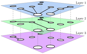
Figure 1: An example of multiplex network with three layers. Each edge belongs to only one layer, whereas each node has one ’copy’ in each layer. Even though, in each separate layer the nodes can be partitioned into different sets of connected components, the network is fully connected in the weak sence, when the connectivity information from all layers is combined.

This section considers the multiplex configuration model: a generalisation of the configuration model in which undirected edges are partitioned into subsets commonly referred to as types, layers, or colors Kivelä et al. (2014). In multiplex networks each edge belongs to one of many layers. Figure 1 illustrates an instance of a three-layer multiplex network with 10 nodes. There are multiple ways to define a path in multiplex networks. A multilayer path, or simply a path in this section of the paper, is a path that combines edges from arbitrary layers. This definition of a path gives rise to a definition of multilayer connected components as sets of nodes connected together with the path.

Suppose, each edge belongs to a layer from Ω={1,,N}.Ω1𝑁\Omega=\{1,\dots,N\}. We update the definition of the degree distribution to be a multivariate function u(k1,,kN),ki0𝑢subscript𝑘1subscript𝑘𝑁subscript𝑘𝑖subscript0u(k_{1},\dots,k_{N}),\;k_{i}\in\mathbb{N}_{0} that denotes probability of randomly choosing a node with kisubscript𝑘𝑖k_{i} adjacent edges of from layer i.𝑖i. As before, the degree distribution is normalised k1,,kNu(k1,,kn)=1.subscriptsubscript𝑘1subscript𝑘𝑁𝑢subscript𝑘1subscript𝑘𝑛1\sum\limits_{k_{1},\dots,k_{N}}u(k_{1},\dots,k_{n})=1. The excess degree distribution associated to the ithsuperscript𝑖thi^{\text{th}} layer is denoted with ui(k1,,kN):=ki+1μiui(k1,,ki+1,,kN),assignsubscript𝑢𝑖subscript𝑘1subscript𝑘𝑁subscript𝑘𝑖1subscript𝜇𝑖subscript𝑢𝑖subscript𝑘1subscript𝑘𝑖1subscript𝑘𝑁u_{i}(k_{1},\dots,k_{N}):=\frac{k_{i}+1}{\mu_{i}}u_{i}(k_{1},\dots,k_{i}+1,\dots,k_{N}), where μi=k1,,kN(ki+1)ui(k1,,ki+1,,kN)subscript𝜇𝑖subscriptsubscript𝑘1subscript𝑘𝑁subscript𝑘𝑖1subscript𝑢𝑖subscript𝑘1subscript𝑘𝑖1subscript𝑘𝑁\mu_{i}=\sum\limits_{k_{1},\dots,k_{N}}(k_{i}+1)u_{i}(k_{1},\dots,k_{i}+1,\dots,k_{N}) is the expected degree for ithsuperscript𝑖thi^{\text{th}}-layer edges. Let w(n)𝑤𝑛w(n) denotes the size distribution for multilayer components. By following similar considerations as in Section III, one derives functional equations for the GF of the size-distribution, W(n)𝑊𝑛W(n):

W(x)𝑊𝑥\displaystyle W(x) =xU[W1(x),,WN(x)],absent𝑥𝑈subscript𝑊1𝑥subscript𝑊𝑁𝑥\displaystyle=xU[W_{1}(x),\dots,W_{N}(x)], (37)
W1(x)subscript𝑊1𝑥\displaystyle W_{1}(x) =xU1[W1(x),,WN(x)],absent𝑥subscript𝑈1subscript𝑊1𝑥subscript𝑊𝑁𝑥\displaystyle=xU_{1}[W_{1}(x),\dots,W_{N}(x)],
WN(x) subscript𝑊𝑁𝑥\displaystyle\dots{\\ }W_{N}(x) =xUN[W1(x),,WN(x)],absent𝑥subscript𝑈𝑁subscript𝑊1𝑥subscript𝑊𝑁𝑥\displaystyle=xU_{N}[W_{1}(x),\dots,W_{N}(x)],

where the upper-case notation U(x1,,xN),𝑈subscript𝑥1subscript𝑥𝑁U(x_{1},\dots,x_{N}), Ui(x1,,xN),i=1,,Nformulae-sequencesubscript𝑈𝑖subscript𝑥1subscript𝑥𝑁𝑖1𝑁U_{i}(x_{1},\dots,x_{N}),\;i=1,\dots,N is used to denote multivariate generating functions of the corresponding distributions. The system of functional equations (37) is a special case of (3), and thus can be solved by applying Lagrange-Good formula. Indeed, let Wi(x)subscript𝑊𝑖𝑥W_{i}(x) define the diagonals of 𝐀i(𝐱)subscript𝐀𝑖𝐱\mathbf{A}_{i}(\mathbf{x}), that is 𝐀i(x,,x):=Wi(x),|x|<1,x,formulae-sequenceassignsubscript𝐀𝑖𝑥𝑥subscript𝑊𝑖𝑥formulae-sequence𝑥1𝑥\mathbf{A}_{i}(x,\dots,x):=W_{i}(x),\,|x|<1,\,x\in\mathbb{C}, for i=1,,N.𝑖1𝑁i=1,\dots,N. Additionally, let 𝐑(𝐱)=[U1(𝐱),,U1(𝐱)],𝐑𝐱subscript𝑈1𝐱subscript𝑈1𝐱\mathbf{R}(\mathbf{x})=[U_{1}(\mathbf{x}),\dots,U_{1}(\mathbf{x})], and F(𝐱)=U(𝐱),𝐹𝐱𝑈𝐱F(\mathbf{x})=U(\mathbf{x}), then the Lagrange-Good formula yields the expression for a(k1,,kN)𝑎subscript𝑘1subscript𝑘𝑁a(k_{1},\dots,k_{N}) that is generated by A(x1,,xN)=1xW(x)𝐴subscript𝑥1subscript𝑥𝑁1𝑥𝑊𝑥A(x_{1},\dots,x_{N})=\frac{1}{x}W(x). The values for w(n)𝑤𝑛w(n) can then be recovered using relation w(n)=k1++kN=n1ki0a(k1,,kN),𝑤𝑛subscriptsubscript𝑘1subscript𝑘𝑁𝑛1subscript𝑘𝑖0𝑎subscript𝑘1subscript𝑘𝑁w(n)=\sum\limits_{\begin{subarray}{c}k_{1}+\dots+k_{N}=n-1\\ k_{i}\geq 0\end{subarray}}a(k_{1},\dots,k_{N}), and the complete equation for component-size distribution in the multilayered configuration network reads: for n>1,𝑛1n>1, w(n)=k1++kN=n1ki0u(𝐤)det[D(𝐤)]u1(𝐤)k1uN(𝐤)kN,𝑤𝑛subscriptsubscript𝑘1subscript𝑘𝑁𝑛1subscript𝑘𝑖0𝑢𝐤subscriptdetdelimited-[]𝐷𝐤subscript𝑢1superscript𝐤absentsubscript𝑘1subscript𝑢𝑁superscript𝐤absentsubscript𝑘𝑁w(n)=\sum_{\begin{subarray}{c}k_{1}+\dots+k_{N}=n-1\\ k_{i}\geq 0\end{subarray}}u(\mathbf{k})*\text{det}_{*}[D(\mathbf{k})]*u_{1}(\mathbf{k})^{*k_{1}}*\dots*u_{N}(\mathbf{k})^{*k_{N}}, (38)
where

D(𝐤)i,j=δi,j[kjui(𝐤)]ui(𝐤)(1),i,j=1,,N,formulae-sequence𝐷subscript𝐤𝑖𝑗subscript𝛿𝑖𝑗delimited-[]subscript𝑘𝑗subscript𝑢𝑖𝐤subscript𝑢𝑖superscript𝐤absent1𝑖𝑗1𝑁D(\mathbf{k})_{i,j}=\delta_{i,j}-[k_{j}u_{i}(\mathbf{k})]*u_{i}(\mathbf{k})^{*(-1)},\;i,j=1,\dots,N,

and det[D(𝐤)]subscriptdetdelimited-[]𝐷𝐤\text{det}_{*}[D(\mathbf{k})] refers to the determinant of matrix D𝐷D computed with the multiplication replaced by the convolution: for example,

det[a(𝐤)b(𝐤)c(𝐤)d(𝐤)]=a(𝐤)d(𝐤)b(𝐤)c(𝐤).𝑑𝑒subscript𝑡matrix𝑎𝐤𝑏𝐤𝑐𝐤𝑑𝐤𝑎𝐤𝑑𝐤𝑏𝐤𝑐𝐤det_{*}\begin{bmatrix}a(\mathbf{k})&b(\mathbf{k})\\ c(\mathbf{k})&d(\mathbf{k})\end{bmatrix}=a(\mathbf{k})*d(\mathbf{k})-b(\mathbf{k})*c(\mathbf{k}).

IV.2 Two-layer multiplex network

Suppose N=2𝑁2N=2, that is to say each edge belongs either to Layer 1 or Layer 2. In this case, the degree distribution d(k,l)𝑑𝑘𝑙d(k,l) is the probability of randomly selecting a node that bears k𝑘k edges in Layer 1 and l𝑙l edges in Layer 2. Where it leads to no confusion, we will reuse the notation from the previous section. For instance, the shorthand notations for moments, vectors of expected values and covariance matrices are as given in (6) and (17) respectively. The total probability is normalised μ00=1,subscript𝜇001\mu_{00}=1, but the expected numbers of edges in each layer need not be the same:

μ10μ01.subscript𝜇10subscript𝜇01\mu_{10}\neq\mu_{01}.

The two dimensional version of (37) reads,

W(x)=xU[W1(x),W2(x)],𝑊𝑥𝑥𝑈subscript𝑊1𝑥subscript𝑊2𝑥W(x)=xU\big{[}W_{\text{1}}(x),W_{\text{2}}(x)\big{]}, (39)
W1(x)=xU1[W1(x),W2(x)],subscript𝑊1𝑥𝑥subscript𝑈1subscript𝑊1𝑥subscript𝑊2𝑥\displaystyle W_{\text{1}}(x)=xU_{\text{1}}\big{[}W_{\text{1}}(x),W_{\text{2}}(x)\big{]}, (39a𝑎a)
W2(x)=xU2[W1(x),W2(x)],subscript𝑊2𝑥𝑥subscript𝑈2subscript𝑊1𝑥subscript𝑊2𝑥\displaystyle W_{\text{2}}(x)=xU_{\text{2}}\big{[}W_{\text{1}}(x),W_{\text{2}}(x)\big{]},

where U(x,y),U1(x,y),U2(x,y)𝑈𝑥𝑦subscript𝑈1𝑥𝑦subscript𝑈2𝑥𝑦U(x,y),U_{1}(x,y),U_{2}(x,y) denote the corresponding generating functions for degree and excess distributions, and W(x)𝑊𝑥W(x) is the generating function for the size distribution of two-layer connected components. The only structural difference between the equation for directed networks Eq. (10) and the equation for two-layered network (39) is the order of arguments in the degree distribution GFs, which indicates presence or absence of symmetric edges (compare Win(x)=xUin[Wout(x),Win(x)]subscript𝑊𝑖𝑛𝑥𝑥subscript𝑈𝑖𝑛subscript𝑊𝑜𝑢𝑡𝑥subscript𝑊𝑖𝑛𝑥W_{in}(x)=xU_{in}[W_{out}(x),W_{in}(x)] against W1(x)=xU1[W1(x),W2(x)]subscript𝑊1𝑥𝑥subscript𝑈1subscript𝑊1𝑥subscript𝑊2𝑥W_{1}(x)=xU_{1}[W_{1}(x),W_{2}(x)]). By setting N=2𝑁2N=2 in (38) one obtains the formal solution to (39),

w(n)=i=0n1a(i,ni1),n>1,formulae-sequence𝑤𝑛superscriptsubscript𝑖0𝑛1𝑎𝑖𝑛𝑖1𝑛1w(n)=\sum\limits_{i=0}^{n-1}a(i,n-i-1),\;n>1, (40)

where for i,j0𝑖𝑗0i,j\geq 0,

a(i,j)=u(k,l)u1(k,l)(i1)u2(k,l)(j1)d(k,l)|k=il=j,𝑎𝑖𝑗evaluated-at𝑢𝑘𝑙subscript𝑢1superscript𝑘𝑙absent𝑖1subscript𝑢2superscript𝑘𝑙absent𝑗1𝑑𝑘𝑙𝑘𝑖𝑙𝑗a(i,j)=u(k,l)*u_{\text{1}}(k,l)^{*(i-1)}*u_{\text{2}}(k,l)^{*(j-1)}*d(k,l)\Big{|}_{\begin{subarray}{c}k=i\\ l=j\end{subarray}}, (41)

and

d(k,l)=[u1(k,l)ku1(k,l)][u2(k,l)lu2(k,l)]lu1(k,l)ku2(k,l).𝑑𝑘𝑙delimited-[]subscript𝑢1𝑘𝑙𝑘subscript𝑢1𝑘𝑙delimited-[]subscript𝑢2𝑘𝑙𝑙subscript𝑢2𝑘𝑙𝑙subscript𝑢1𝑘𝑙𝑘subscript𝑢2𝑘𝑙d(k,l)=[u_{\text{1}}(k,l)-ku_{\text{1}}(k,l)]*[u_{\text{2}}(k,l)-lu_{\text{2}}(k,l)]\\ -lu_{\text{1}}(k,l)*ku_{\text{2}}(k,l). (42)

We will now see how the asymptotic theory from Section III.4 can be recast to fit the case of the two-layer multiplex networks.

IV.3 Asymptotic analysis for a bilayer network

Let μ1,μ2subscript𝜇1subscript𝜇2\mu_{1},\mu_{2} denote expected values and Σ1,Σ2subscriptΣ1subscriptΣ2\Sigma_{1},\Sigma_{2} covariance matrices of kμ10u(k,l)𝑘subscript𝜇10𝑢𝑘𝑙\frac{k}{\mu_{10}}u(k,l) and lμ01u(k,l),𝑙subscript𝜇01𝑢𝑘𝑙\frac{l}{\mu_{01}}u(k,l), as given in definition (17). The characteristic function for the right hand side of Eq. (41) reads: ϕasubscriptitalic-ϕ𝑎\displaystyle\phi_{a} (ω1,ω2)=ei(iω1+jω2)ϕ(ω1,ω2)subscript𝜔1subscript𝜔2superscript𝑒i𝑖subscript𝜔1𝑗subscript𝜔2italic-ϕsubscript𝜔1subscript𝜔2\displaystyle(\omega_{1},\omega_{2})=e^{-\mathrm{i}\mkern 1.0mu(i\omega_{1}+j\omega_{2})}\phi(\omega_{1},\omega_{2}) (43) ×\displaystyle\times ([iμ1ω1ϕ(ω1,ω2)]i[iμ2ω2ϕ(ω1,ω2)]j\displaystyle\left(\left[-\frac{\mathrm{i}\mkern 1.0mu}{\mu_{1}}\frac{\partial}{\partial\omega_{1}}\phi(\omega_{1},\omega_{2})\right]^{i}\left[-\frac{\mathrm{i}\mkern 1.0mu}{\mu_{2}}\frac{\partial}{\partial\omega_{2}}\phi(\omega_{1},\omega_{2})\right]^{j}\right. +ijω2[iμ1ω1ϕ(ω1,ω2)]i[iμ2ω2ϕ(ω1,ω2)]ji𝑗subscript𝜔2superscriptdelimited-[]isubscript𝜇1subscript𝜔1italic-ϕsubscript𝜔1subscript𝜔2𝑖superscriptdelimited-[]isubscript𝜇2subscript𝜔2italic-ϕsubscript𝜔1subscript𝜔2𝑗\displaystyle+\frac{\mathrm{i}\mkern 1.0mu}{j}\frac{\partial}{\partial\omega_{2}}\left[-\frac{\mathrm{i}\mkern 1.0mu}{\mu_{1}}\frac{\partial}{\partial\omega_{1}}\phi(\omega_{1},\omega_{2})\right]^{i}\left[-\frac{\mathrm{i}\mkern 1.0mu}{\mu_{2}}\frac{\partial}{\partial\omega_{2}}\phi(\omega_{1},\omega_{2})\right]^{j} +ii[iμ1ω1ϕ(ω1,ω2)]iω1[iμ2ω2ϕ(ω1,ω2)]ji𝑖superscriptdelimited-[]isubscript𝜇1subscript𝜔1italic-ϕsubscript𝜔1subscript𝜔2𝑖subscript𝜔1superscriptdelimited-[]isubscript𝜇2subscript𝜔2italic-ϕsubscript𝜔1subscript𝜔2𝑗\displaystyle+\frac{\mathrm{i}\mkern 1.0mu}{i}\left[-\frac{\mathrm{i}\mkern 1.0mu}{\mu_{1}}\frac{\partial}{\partial\omega_{1}}\phi(\omega_{1},\omega_{2})\right]^{i}\frac{\partial}{\partial\omega_{1}}\left[-\frac{\mathrm{i}\mkern 1.0mu}{\mu_{2}}\frac{\partial}{\partial\omega_{2}}\phi(\omega_{1},\omega_{2})\right]^{j} 1ijω2[iμ1ω1ϕ(ω1,ω2)]iω1[iμ2ω2ϕ(ω1,ω2)]j1𝑖𝑗subscript𝜔2superscriptdelimited-[]isubscript𝜇1subscript𝜔1italic-ϕsubscript𝜔1subscript𝜔2𝑖subscript𝜔1superscriptdelimited-[]isubscript𝜇2subscript𝜔2italic-ϕsubscript𝜔1subscript𝜔2𝑗\displaystyle-\frac{1}{ij}\frac{\partial}{\partial\omega_{2}}\left[-\frac{\mathrm{i}\mkern 1.0mu}{\mu_{1}}\frac{\partial}{\partial\omega_{1}}\phi(\omega_{1},\omega_{2})\right]^{i}\frac{\partial}{\partial\omega_{1}}\left[-\frac{\mathrm{i}\mkern 1.0mu}{\mu_{2}}\frac{\partial}{\partial\omega_{2}}\phi(\omega_{1},\omega_{2})\right]^{j} +1ijω1[iμ1ω1ϕ(ω1,ω2)]iω2[iμ2ω2ϕ(ω1,ω2)]j).\displaystyle+\left.\frac{1}{ij}\frac{\partial}{\partial\omega_{1}}\left[-\frac{\mathrm{i}\mkern 1.0mu}{\mu_{1}}\frac{\partial}{\partial\omega_{1}}\phi(\omega_{1},\omega_{2})\right]^{i}\frac{\partial}{\partial\omega_{2}}\left[-\frac{\mathrm{i}\mkern 1.0mu}{\mu_{2}}\frac{\partial}{\partial\omega_{2}}\phi(\omega_{1},\omega_{2})\right]^{j}\right). In the large n𝑛n limit, the latter approaches a(i,j)=C(x)e12xΣ1x2πdet(Σ),subscript𝑎𝑖𝑗𝐶𝑥superscript𝑒12superscript𝑥topsuperscriptΣ1𝑥2𝜋Σa_{\infty}(i,j)=C(x)\frac{e^{-\frac{1}{2}x^{\top}\!\Sigma^{-1}x}}{2\pi\sqrt{\det(\Sigma)}},\\ (44) where x=2(i,j)(iμ1+jμ2)+μ0𝑥2𝑖𝑗𝑖superscriptsubscript𝜇1top𝑗superscriptsubscript𝜇2topsubscript𝜇0x=2(i,j)-(i\mu_{1}^{\top}\!+j\mu_{2}^{\top}\!)+\mu_{0} and C(x)=𝐶𝑥absent\displaystyle C(x)= C0+C1xn+xnC2xn,subscript𝐶0subscript𝐶1𝑥𝑛superscript𝑥top𝑛subscript𝐶2𝑥𝑛\displaystyle C_{0}+C_{1}\frac{x}{n}+\frac{x^{\top}\!}{n}C_{2}\frac{x}{n}, (45) C0=subscript𝐶0absent\displaystyle C_{0}= 42(I1μ1+I2μ2)μ1Dμ2,42subscript𝐼1subscript𝜇1subscript𝐼2subscript𝜇2subscript𝜇1𝐷subscript𝜇2\displaystyle 4-2(I_{1}\mu_{1}+I_{2}\mu_{2})-\mu_{1}D\mu_{2}, C1=subscript𝐶1absent\displaystyle C_{1}= [μ2DΣ1μ1DΣ22(I1Σ1+I2Σ2)](1nΣ)1,delimited-[]superscriptsubscript𝜇2top𝐷subscriptΣ1superscriptsubscript𝜇1top𝐷subscriptΣ22superscriptsubscript𝐼1topsubscriptΣ1superscriptsubscript𝐼2topsubscriptΣ2superscript1𝑛Σ1\displaystyle[\mu_{2}^{\top}\!D\Sigma_{1}-\mu_{1}^{\top}\!D\Sigma_{2}-2(I_{1}^{\top}\!\Sigma_{1}+I_{2}^{\top}\!\Sigma_{2})]\left(\frac{1}{n}\Sigma\right)^{-1}, C2=subscript𝐶2absent\displaystyle C_{2}= (1nΣ)1Σ1DΣ2(1nΣ)1,superscript1𝑛Σ1subscriptΣ1𝐷subscriptΣ2superscript1𝑛Σ1\displaystyle-\left(\frac{1}{n}\Sigma\right)^{-1}\Sigma_{1}D\Sigma_{2}\left(\frac{1}{n}\Sigma\right)^{-1}, Σ=Σabsent\displaystyle\Sigma= iΣ1+jΣ2.𝑖subscriptΣ1𝑗subscriptΣ2\displaystyle i\Sigma_{1}+j\Sigma_{2}.

By applying the change of variables (25), one obtains x=n(az+b+μ0n)𝑥𝑛𝑎𝑧𝑏subscript𝜇0𝑛x=n(az+b+\frac{\mu_{0}}{n}) and Σ=n(Az+B)Σ𝑛𝐴𝑧𝐵\Sigma=n(Az+B) where

a𝑎\displaystyle a =I1I2+μ1μ22,absentsubscript𝐼1subscript𝐼2subscript𝜇1subscript𝜇22\displaystyle=I_{1}-I_{2}+\frac{\mu_{1}-\mu_{2}}{2}, (46)
b𝑏\displaystyle b =1μ1+μ22,absent1subscript𝜇1subscript𝜇22\displaystyle=1-\frac{\mu_{1}+\mu_{2}}{2},
A𝐴\displaystyle A =Σ1Σ22,absentsubscriptΣ1subscriptΣ22\displaystyle=\frac{\Sigma_{1}-\Sigma_{2}}{2},
B𝐵\displaystyle B =Σ1+Σ22.absentsubscriptΣ1subscriptΣ22\displaystyle=\frac{\Sigma_{1}+\Sigma_{2}}{2}.

Now, coefficients C0,C1,C2subscript𝐶0subscript𝐶1subscript𝐶2C_{0},C_{1},C_{2} and 1nΣ=Az+B1𝑛Σ𝐴𝑧𝐵\frac{1}{n}\Sigma=Az+B became independent of n,𝑛n, and Eq. (44) is identical to (24) up to the definitions of constants a,b,A,B,C0,C1,C2,𝑎𝑏𝐴𝐵subscript𝐶0subscript𝐶1subscript𝐶2a,b,A,B,C_{0},C_{1},C_{2}, that are given above. Therefore, we can readily use the asymptote (32) also in the case of a two-layer networks. It is enough to redefine the constants according to definitions (45) and (46) and take z=r1𝑧subscript𝑟1z=r_{1}, where r1[1,1]subscript𝑟111r_{1}\in[-1,1] denotes the root of Eq. (31). As before, condition abba=0𝑎superscript𝑏top𝑏superscript𝑎top0ab^{\top}\!-ba^{\top}\!=0 indicates the emergence of the algebraic decay n32superscript𝑛32n^{-\frac{3}{2}} in the sizes of connected components. When the latter equality is expanded according to definitions (46) and (17), one obtains the criterion in terms of degree distribution moments:

G(u):=μ112(μ202μ10)(μ022μ01)=0.assign𝐺𝑢superscriptsubscript𝜇112subscript𝜇202subscript𝜇10subscript𝜇022subscript𝜇010G(u):=\mu_{11}^{2}-(\mu_{20}-2\mu_{10})(\mu_{02}-2\mu_{01})=0. (47)

As in the case of directed networks, the degenerate excess degree distribution, u1(k,l)=0,k>0,formulae-sequencesubscript𝑢1𝑘𝑙0𝑘0u_{1}(k,l)=0,\;k>0, renders the asymptotic analysis not applicable. Nevertheless, the degenerate case is equivalent to a one-layer network with coupled nodes that has a univariate degree distribution d(l)=d(0,l)+12d(1,l),l=0,formulae-sequence𝑑𝑙𝑑0𝑙12𝑑1𝑙𝑙0d(l)=d(0,l)+\frac{1}{2}d(1,l),\;l=0,\dots The asymptotic theory for mono-layer components has been covered in Ref. Kryven (2017a), and, unlike in the case of directed networks, no new asymptotic modes emerge when the excess distribution is degenerate.

IV.4 Criticality in two-layer multiplex networks

When a configuration network is a two-layered, one may speak of a connected component contained within a specific layer: a path comprise solely of edges from one layer, or a multilayer (weak) connected component that emerges from a combination of two layers: both types of edges may appear in the path. No matter what type of connected components is considered, the asymptote of the component size distribution exhibits either exponential or algebraic decays.

When focusing on single-layer connected components, for instance, in Layer 1, condition μ202μ10=0subscript𝜇202subscript𝜇100\mu_{20}-2\mu_{10}=0 signifies the critical regime of the corresponding size distribution. Furthermore, a giant component exists within this layer iff μ202μ10>0subscript𝜇202subscript𝜇100\mu_{20}-2\mu_{10}>0. Existence of a giant component within a single layer is a strong condition: it automatically implies existence of the weak two-layer giant component. More importantly, the two-layer giant component can also exist even when there are no single-layer giant components.

When two-layered connected components are considered, criterion (47) gives the condition for the algebraic decay in the component-size distribution. It is important to note that one should consider this inequality only together with the validity conditions of the asymptotic theory: μij<,i+j3formulae-sequencesubscript𝜇𝑖𝑗𝑖𝑗3\mu_{ij}<\infty,\;i+j\leq 3 and existence of the root of Eq. (30), |r1|1subscript𝑟11|r_{1}|\leq 1. For instance, unlike in the case of a single layer network, one cannot associate existence of the two-layer giant component solely with the sign of the left hand side of Eq. (47). For a simple contra example, set μ11=0.subscript𝜇110\mu_{11}=0. Then, the left hand side of Eq. (47) is positive iff one layer contains a giant component and the other – does not. When both layers contain a giant component simultaneously (or both layers contain no giant component), the sign is negative.

Now, let us consider a critical degree distribution uc(k,l)subscript𝑢𝑐𝑘𝑙u_{c}(k,l) such that G(uc)=0𝐺subscript𝑢𝑐0G(u_{c})=0 and μ11>0.subscript𝜇110\mu_{11}>0. Assume, there are no single-layer giant components, that is to say 2μ10μ202subscript𝜇10subscript𝜇202\mu_{10}-\mu_{20} and 2μ01μ022subscript𝜇01subscript𝜇022\mu_{01}-\mu_{02} are positive quantities. The upper bounds on these quantities can be obtained from the Cauchy-Schwarz inequality, μ112μ20μ02.superscriptsubscript𝜇112subscript𝜇20subscript𝜇02\mu_{11}^{2}\leq\mu_{20}\mu_{02}. The latter, when combined with condition G(uc)=0𝐺subscript𝑢𝑐0G(u_{c})=0 yields

0<2μ10μ20μ10μ02μ01, 0<2μ01μ02μ01μ20μ10.formulae-sequence02subscript𝜇10subscript𝜇20subscript𝜇10subscript𝜇02subscript𝜇01 02subscript𝜇01subscript𝜇02subscript𝜇01subscript𝜇20subscript𝜇100<2\mu_{10}-\mu_{20}\leq\frac{\mu_{10}\mu_{02}}{\mu_{01}},\;0<2\mu_{01}-\mu_{02}\leq\frac{\mu_{01}\mu_{20}}{\mu_{10}}. (48)

Since there are no isolated nodes, u(k,l)=0,k,l=0,formulae-sequence𝑢𝑘𝑙0𝑘𝑙0u(k,l)=0,\;k,l=0, the sum of expected numbers of edges is bounded below with

μ10+μ011.subscript𝜇10subscript𝜇011\mu_{10}+\mu_{01}\geq 1. (49)

Additionally, one obtains the following bounds from the monotonicity of the moments,

μ20<μ102,μ02<μ012.formulae-sequencesubscript𝜇20superscriptsubscript𝜇102subscript𝜇02superscriptsubscript𝜇012\mu_{20}<\mu_{10}^{2},\;\mu_{02}<\mu_{01}^{2}. (50)

Let us perturb expected number of edges μ10subscript𝜇10\mu_{10} by uniformly adding (or removing) a small number of edges dαd𝛼\text{d}\alpha in the first layer. Due to this perturbation, the degree distribution variates as du(k,l)=[u(k1,l)u(k,l)]dα.d𝑢𝑘𝑙delimited-[]𝑢𝑘1𝑙𝑢𝑘𝑙d𝛼\text{d}u(k,l)=[u(k-1,l)-u(k,l)]\text{d}\alpha. The perturbation conserves the total probability, k,l=0du(k,l)=0,superscriptsubscript𝑘𝑙0d𝑢𝑘𝑙0\sum\limits_{k,l=0}^{\infty}\text{d}u(k,l)=0, whereas the expected number of edges, indeed, variates as dμ10=k,l=0k[u(k1,l)u(k,l)]dα=k,l=0[(k+1)u(k,l)ku(k,l)]dα=dαdsubscript𝜇10superscriptsubscript𝑘𝑙0𝑘delimited-[]𝑢𝑘1𝑙𝑢𝑘𝑙d𝛼superscriptsubscript𝑘𝑙0delimited-[]𝑘1𝑢𝑘𝑙𝑘𝑢𝑘𝑙d𝛼d𝛼\text{d}\mu_{10}=\sum\limits_{k,l=0}^{\infty}k[u(k-1,l)-u(k,l)]\,\text{d}\alpha=\sum\limits_{k,l=0}^{\infty}[(k+1)u(k,l)-ku(k,l)]\,\text{d}\alpha=\text{d}\alpha. After expanding variations dμ11=μ01dαdsubscript𝜇11subscript𝜇01d𝛼\text{d}\mu_{11}=\mu_{01}\text{d}\alpha and dμ20=(2μ10+1)dαdsubscript𝜇202subscript𝜇101d𝛼\text{d}\mu_{20}=(2\mu_{10}+1)\text{d}\alpha in a similar fashion, we write the Gâteaux derivative,

ddαG(uc)=limdα0G(uc+du)G(uc)dα=(μ11+μ01dα)2[μ20+(2μ10+1)dα2(μ10+dα)](μ022μ01)=(2μ01μ02)(2μ101)+2μ01μ11.d𝑑𝛼𝐺subscript𝑢𝑐subscriptd𝛼0𝐺subscript𝑢𝑐d𝑢𝐺subscript𝑢𝑐d𝛼superscriptsubscript𝜇11subscript𝜇01d𝛼2delimited-[]subscript𝜇202subscript𝜇101d𝛼2subscript𝜇10d𝛼subscript𝜇022subscript𝜇012subscript𝜇01subscript𝜇022subscript𝜇1012subscript𝜇01subscript𝜇11\frac{\text{d}}{d\alpha}G(u_{c})=\lim\limits_{\text{d}\alpha\to 0}\frac{G(u_{c}+\text{d}u)-G(u_{c})}{\text{d}\alpha}=\\ (\mu_{11}+\mu_{01}\text{d}\alpha)^{2}-[\mu_{20}+(2\mu_{10}+1)\text{d}\alpha-2(\mu_{10}+\text{d}\alpha)](\mu_{02}-2\mu_{01})=\\ (2\mu_{01}-\mu_{02})(2\mu_{10}-1)+2\mu_{01}\mu_{11}.

We will now show that ddαG(uc)>0d𝑑𝛼𝐺subscript𝑢𝑐0\frac{\text{d}}{d\alpha}G(u_{c})>0 by considering two cases. Firstly, let 2μ1010,2subscript𝜇10102\mu_{10}-1\geq 0, then (2μ01μ02)>02subscript𝜇01subscript𝜇020(2\mu_{01}-\mu_{02})>0 according to (48), and consequently, ddαG(uc)>0.d𝑑𝛼𝐺subscript𝑢𝑐0\frac{\text{d}}{d\alpha}G(u_{c})>0. Secondly, let us assume the opposite is true, 0<μ10<12::0subscript𝜇1012absent0<\mu_{10}<\frac{1}{2}: by expressing μ11subscript𝜇11\mu_{11} from (47) and plugging it into ddαG(uc)>0d𝑑𝛼𝐺subscript𝑢𝑐0\frac{\text{d}}{d\alpha}G(u_{c})>0 one obtains

μ01(2μ10μ20)1μ01(2μ01μ02)(12μ10)2>0.subscript𝜇012subscript𝜇10subscript𝜇201subscript𝜇012subscript𝜇01subscript𝜇02superscript12subscript𝜇1020\mu_{01}(2\mu_{10}-\mu_{20})-\frac{1}{\mu_{01}}(2\mu_{01}-\mu_{02})(1-2\mu_{10})^{2}>0. (51)

Combining lower bound μ011μ10=12subscript𝜇011subscript𝜇1012\mu_{01}\geq 1-\mu_{10}=\frac{1}{2} (as follows from (49)) and the upper bound on μ20subscript𝜇20\mu_{20} (as given in (50)), the first term in (51) is bounded below with μ01(2μ10μ20)12(2μ10μ102).subscript𝜇012subscript𝜇10subscript𝜇20122subscript𝜇10superscriptsubscript𝜇102\mu_{01}(2\mu_{10}-\mu_{20})\geq\frac{1}{2}(2\mu_{10}-\mu_{10}^{2}). The lower bound for the second term of (51) follows from sequentially applying (48) and (50):

1μ01(2μ01μ02)(12μ10)2μ20μ10(12μ10)2μ10(12μ10)2.1subscript𝜇012subscript𝜇01subscript𝜇02superscript12subscript𝜇102subscript𝜇20subscript𝜇10superscript12subscript𝜇102subscript𝜇10superscript12subscript𝜇102-\frac{1}{\mu_{01}}(2\mu_{01}-\mu_{02})(1-2\mu_{10})^{2}\geq\\ -\frac{\mu_{20}}{\mu_{10}}(1-2\mu_{10})^{2}\geq\\ -\mu_{10}(1-2\mu_{10})^{2}. (52)

So that

μ01(2μ10μ20)1μ01(2μ01μ02)(12μ10)212(2μ10μ102)μ10(12μ10)2=12(78μ10)μ102>32μ102>0.subscript𝜇012subscript𝜇10subscript𝜇201subscript𝜇012subscript𝜇01subscript𝜇02superscript12subscript𝜇102122subscript𝜇10superscriptsubscript𝜇102subscript𝜇10superscript12subscript𝜇1021278subscript𝜇10superscriptsubscript𝜇10232superscriptsubscript𝜇1020\mu_{01}(2\mu_{10}-\mu_{20})-\frac{1}{\mu_{01}}(2\mu_{01}-\mu_{02})(1-2\mu_{10})^{2}\geq\\ \frac{1}{2}(2\mu_{10}-\mu_{10}^{2})-\mu_{10}(1-2\mu_{10})^{2}=\frac{1}{2}(7-8\mu_{10})\mu_{10}^{2}>\frac{3}{2}\mu_{10}^{2}>0. (53)

The fact that ddαG(uc)>0d𝑑𝛼𝐺subscript𝑢𝑐0\frac{\text{d}}{d\alpha}G(u_{c})>0 means that perturbing the configuration network at the critical regime, G(u)=0,𝐺𝑢0G(u)=0, by a uniform addition of new edges forces the value of G(u)𝐺𝑢G(u) to become positive. The opposite is also true: uniform removal of existing edges at the critical regime forces values of G(u)𝐺𝑢G(u) to become negative. Similar derivation holds for the perturbation in the second layer.

Finally, suppose one modifies u(k,l)𝑢𝑘𝑙u(k,l) in such a manner that the expected numbers of edges, μ10,μ01subscript𝜇10subscript𝜇01\mu_{10},\mu_{01} remain constant whereas the second moments alter. Such a perturbation of the degree distribution causes rewiring of the network but keeps the expected numbers of edges in each layer the same. Consider a function f(μ20,μ02):=μ112(μ202μ10)(μ022μ01)=G(uc),assign𝑓subscript𝜇20subscript𝜇02superscriptsubscript𝜇112subscript𝜇202subscript𝜇10subscript𝜇022subscript𝜇01𝐺subscript𝑢𝑐f(\mu_{20},\mu_{02}):=\mu_{11}^{2}-(\mu_{20}-2\mu_{10})(\mu_{02}-2\mu_{01})=G(u_{c}), as follows from the lower bounds (48), both components of the gradient vector,

f(μ20,μ02)=(2μ01μ02,2μ10μ20),𝑓subscript𝜇20subscript𝜇022subscript𝜇01subscript𝜇022subscript𝜇10subscript𝜇20\nabla f(\mu_{20},\mu_{02})=(2\mu_{01}-\mu_{02},2\mu_{10}-\mu_{20}),

are positive. This fact confirms that rewiring that moves edges within a single layer toward the nodes with higher degree forces the value of G(u)𝐺𝑢G(u) to become positive. The total action of the simultaneous rewiring in two layers is defined by sign[(2μ01μ02,2μ10μ20)(μ20,μ02)].signdelimited-[]superscript2subscript𝜇01subscript𝜇022subscript𝜇10subscript𝜇20topsubscript𝜇20subscript𝜇02\text{sign}[(2\mu_{01}-\mu_{02},2\mu_{10}-\mu_{20})^{\top}\!(\partial\mu_{20},\partial\mu_{02})].

According to the asymptote (32), if G(u)=0𝐺𝑢0G(u)=0, the size distribution decays algebraically with exponent 32,32-\frac{3}{2}, and therefore, expected component size diverges. On one hand, perturbations of the network by inflection with new edges or a rewiring that moves edges to nodes with larger degree does not reduce the size of the largest component, on the other hand, after such a perturbation G(u)0𝐺𝑢0G(u)\neq 0: the component-size distribution switches to the exponential decay and features finite expected component size. The deficit in expected component size, which due to the nature of the perturbation could have only increased if all connected components were finite, is attributed to the emergence of the giant two-layer component.
Refer to caption
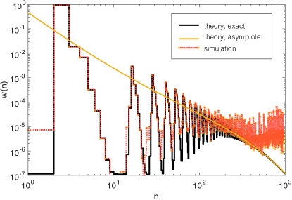
Figure 2: (color online) An oscillatory example of the size distribution of connected components in the two-layer configuration model as predicted by the analytical expression (40) (solid black line) is compared against the data obtained from simulations (scattered points linked with a dashed line that indicates the trend). Low probabilities are naturally underrepresented in simulated data due to a limited size of the Monte Carlo sample. The theory, as given by Eqs. (32) and (45), predicts the asymptote with a transient slope 3232-\frac{3}{2} (solid yellow line).
Refer to caption
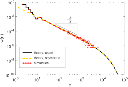
Figure 3: (color online) An example of the size distribution of weakly connected components in a directed configuration model as predicted by the analytical expression (15) (solid line) is compared against the data obtained from simulations (scattered points). The theory, as given by Eq. (32), predicts the asymptote with a transient slope 3232-\frac{3}{2} (dashed line).
Refer to caption
Figure 4: (color online) An example of the size distribution of weakly connected components in a directed configuration model as predicted by the analytical expression (15) (solid line) is compared against the data obtained from simulations (scattered points). The theory, as given by Eq. (36), predicts the asymptote with a transient slope 1212-\frac{1}{2} (dashed line).

V Discussion and conclusions

The main results of this study are the formal expressions for the size distributions of connected components in directed and multiplex networks. These expressions involve the convolution power and, in practice, can be evaluated exactly with FFT algorithm in the cost of O(n2logn),𝑂superscript𝑛2𝑛O(n^{2}\log n), in the case of directed networks, and O(nNlogn),𝑂superscript𝑛𝑁𝑛O(n^{N}\log n), in the case of multiplex networks with 1<N<n1𝑁𝑛1<N<n layers. These expressions are very general and do not rely upon any restrictions on the degree distribution itself. The supporting code is accessible at GitHub repository git . Unlike the fixed point formulations (10),(39), the formal expressions for component size distributions are tractable from asymptotic theory point of view. The asymptotic analysis for weak/multilayer connected components resulted in simple analytical expressions that, under certain conditions, feature a self-similar behaviour. The asymptotic theory, however, does rely on a few assumptions that to a certain extent limit the space of applicable degree distributions. First, we assume finiteness of partial moments, μij<,i+j3;formulae-sequencesubscript𝜇𝑖𝑗𝑖𝑗3\mu_{ij}<\infty,\;i+j\leq 3; second, we rely upon existence of the real root of Eq. (30) such that |r1|1.subscript𝑟11|r_{1}|\leq 1. Finally, there is a practical restriction that arises if one aims to utilise the asymptote as an approximation for the size distribution itself: the best approximation accuracy is gained when the network is in the critical window |ar1+b|=ϵ,𝑎subscript𝑟1𝑏italic-ϵ|ar_{1}+b|=\epsilon, where ϵitalic-ϵ\epsilon is infinitesimal.

A few examples of size distributions of connected components and corresponding to them analytical asymptotes are given in Figs. 23 and 4. Figure 2 compares the new theory against simulated data for the case of a two-layer network with the degree distribution given by

u(k,l)=0.9782e5[(k1)2+l2)]+0.002e10[(k9)2+(l3)2].u(k,l)=0.9782e^{-5[(k-1)^{2}+l^{2})]}+0.002e^{-10[(k-9)^{2}+(l-3)^{2}]}.

This example was selected to demonstrates the possibility of an oscillatory behaviour arising in the size distribution of connected components. It can be noted that the theory, as given by Eq. (40), accurately predicts the non-trivial oscillations present in the data. For large n𝑛n, the theoretical predictions in this example converge to the asymptote, as given by Eq. (32).

Figure 3 features the size distribution of connected components in a directed network featuring a non-degenerate degree distribution,

u(k,l)=0.5167ek2l2+0.0052e2.5[(k4)2+(l4)2],𝑢𝑘𝑙0.5167superscript𝑒superscript𝑘2superscript𝑙20.0052superscript𝑒2.5delimited-[]superscript𝑘42superscript𝑙42u(k,l)=0.5167e^{-k^{2}-l^{2}}+0.0052e^{-2.5[(k-4)^{2}+(l-4)^{2}]},

whereas Fig. 4 features the results obtained for a degenerate degree distribution:

u(0,k)𝑢0𝑘\displaystyle u(0,k) =0.9073e2.266k,k0,formulae-sequenceabsent0.9073superscript𝑒2.266𝑘𝑘0\displaystyle=0.9073e^{-2.266k},\;k\geq 0,
u(1,k)𝑢1𝑘\displaystyle u(1,k) =0.9073e0.7k,k0,formulae-sequenceabsent0.9073superscript𝑒0.7𝑘𝑘0\displaystyle=0.9073e^{-0.7k},\;k\geq 0,
u(l,k)𝑢𝑙𝑘\displaystyle u(l,k) =0,l>1,k0.formulae-sequenceabsent0formulae-sequence𝑙1𝑘0\displaystyle=0,\;l>1,k\geq 0.

As in the previous example, both Figs. 3 and 4 compare the theoretical size distribution, as given by Eq. (15), to the simulated data. In both figures, the theoretical predictions and the data converge to the asymptotes for large n𝑛n. In the case of the non-degenerate degree distribution, the asymptote features transient slope 3232-\frac{3}{2}, as predicted by Eq. (32). However, in the case of the degenerate degree distribution the transient slope of the asymptote is 1212-\frac{1}{2}, which is in accordance with Eq. (36). The latter observation is a surprising result. This is the first evidence that a configuration model with a light-tailed degree distribution may feature a distinct from 3232-\frac{3}{2} exponent. Importantly, in the multiplex configuration network with two layers such an anomaly is not present. When the degree distribution is light-tailed, both non-degenerate directed networks and two-layer networks feature leading exponent 3232-\frac{3}{2} in the critical regime, which is also the case in undirected networks.

A comparison of the theory agains a few examples of empirical data is given in Fig. 5. This figure presents normalised to the number of nodes theoretical size distributions of weakly connected components and compares them to empirical component-count distributions extracted from various datasets of directed networks.

a. Refer to caption b. Refer to caption c. Refer to caption

Figure 5: (color online) Comparisons of respective theoretical size distributions of finite components against the empirical data. Three cases of directed networks containing N𝑁N nodes in total are considered: a. the network of retweets in the Higgs/Twitter dataset, N=425 008𝑁425008N=425\,008 De Domenico et al. (2013b); b. the graph of the sparse statistical matrix Chem97ZtZ, N=2 541𝑁2541N=2\,541 Davis and Hu (2011); c. the network of communications on Wikipedia till January 2008, N=2 394 385𝑁2394385N=2\,394\,385 Leskovec et al. (2010).

In undirected, single-layer configuration networks, a heavy tail in the size distribution is observed when μ22μ1=0subscript𝜇22subscript𝜇10\mu_{2}-2\mu_{1}=0, where μ2subscript𝜇2\mu_{2} and μ1subscript𝜇1\mu_{1} are the moments of the univariate degree distribution. Furthermore, when the equality sign in this criterion is replaced by the inequality sign, μ22μ1>0,subscript𝜇22subscript𝜇10\mu_{2}-2\mu_{1}>0, one obtains the criterion for giant component existence. Similar inequality criterion can be constructed for directed networks: also in this case the condition for a heavy tail in the size distribution relates to the giant component existence Kryven (2016). However, this principle breaks down already in multiplex networks that consist of as few as two layers. The sign of the left hand side of the criticality condition (47) cannot be directly associated with existence of the giant two-layer component. Nevertheless, as was argued in Section IV.4, if equality (47) fails to hold due to a small perturbation in the expected numbers of edges μ10,μ01subscript𝜇10subscript𝜇01\mu_{10},\mu_{01} (or rewiring caused by an increase of second moments μ20,μ02subscript𝜇20subscript𝜇02\mu_{20},\mu_{02}) at the critical regime, one can still associate the sign of the left hand side in Eq. (47) with the giant component existence. This association is guaranteed to be valid within the critical window.
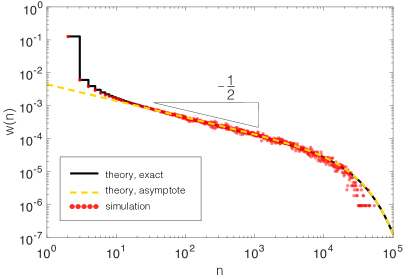
Acknowledgements.
This work is part of the project number 639.071.511, which is financed by the Netherlands Organisation for Scientific Research (NWO) VENI.

References

  • Kivelä et al. (2014) M. Kivelä, A. Arenas, M. Barthelemy, J. P. Gleeson, Y. Moreno,  and M. A. Porter, Journal of complex networks 2, 203 (2014).
  • Nicosia et al. (2013) V. Nicosia, G. Bianconi, V. Latora,  and M. Barthelemy, Physical review letters 111, 058701 (2013).
  • Kleineberg et al. (2016) K.-K. Kleineberg, M. Boguna, M. Angeles Serrano,  and F. Papadopoulos, Nat Phys 12, 1076 (2016).
  • Cardillo et al. (2013) A. Cardillo, J. Gómez-Gardenes, M. Zanin, M. Romance, D. Papo, F. Del Pozo,  and S. Boccaletti, Scientific reports 3, 1344 (2013).
  • Newman (2002) M. E. J. Newman, Physical review letters 89, 208701 (2002).
  • Bender and Canfield (1978) E. A. Bender and E. R. Canfield, Journal of Combinatorial Theory, Series A 24, 296 (1978).
  • Molloy and Reed (1995) M. Molloy and B. Reed, Random structures & algorithms 6, 161 (1995).
  • Newman et al. (2001) M. E. J. Newman, S. H. Strogatz,  and D. J. Watts, Physical review E 64, 026118 (2001).
  • Newman (2007) M. E. J. Newman, Phys. Rev. E 76, 045101 (2007).
  • Shi et al. (2009) Y. Y. Shi, H. Qian, et al., Communications in Mathematical Sciences 7, 175 (2009).
  • Kryven (2016) I. Kryven, Phys. Rev. E 94, 012315 (2016).
  • Bianconi et al. (2015) G. Bianconi, S. N. Dorogovtsev,  and J. F. F. Mendes, Phys. Rev. E 91, 012804 (2015).
  • Azimi-Tafreshi et al. (2014) N. Azimi-Tafreshi, J. Gómez-Gardenes,  and S. N. Dorogovtsev, Physical Review E 90, 032816 (2014).
  • Cellai et al. (2013) D. Cellai, E. López, J. Zhou, J. P. Gleeson,  and G. Bianconi, Physical Review E 88, 052811 (2013).
  • Bianconi (2013) G. Bianconi, Physical Review E 87, 062806 (2013).
  • Baxter et al. (2014) G. J. Baxter, S. N. Dorogovtsev, J. F. F. Mendes,  and D. Cellai, Physical Review E 89, 042801 (2014).
  • De Domenico et al. (2013a) M. De Domenico, A. Solé-Ribalta, E. Cozzo, M. Kivelä, Y. Moreno, M. A. Porter, S. Gómez,  and A. Arenas, Physical Review X 3, 041022 (2013a).
  • Kryven (2017a) I. Kryven, Phys. Rev. E 95, 052303 (2017a).
  • Kryven (2017b) I. Kryven, Journal of Mathematical Chemistry , 10.1007/s10910 (2017b).
  • Hackett et al. (2016) A. Hackett, D. Cellai, S. Gómez, A. Arenas,  and J. P. Gleeson, Physical Review X 6, 021002 (2016).
  • Bergeron et al. (1998) F. Bergeron, G. Labelle,  and P. Leroux, Combinatorial species and tree-like structures (Cambridge University Press, Cambridge, UK, 1998).
  • Good (1960) I. J. Good, in Mathematical Proceedings of the Cambridge Philosophical Society, Vol. 56 (Cambridge Univ Press, 1960) pp. 367–380.
  • (23) “Matlab/GNU Octave source code for cacluating size distributions of weakly connected components,” github.com/ikryven/PhysRevE_2017_MultiDirNet.
  • De Domenico et al. (2013b) M. De Domenico, A. Lima, P. Mougel,  and M. Musolesi, Scientific reports 3, 2980 (2013b).
  • Davis and Hu (2011) T. A. Davis and Y. Hu, ACM Transactions on Mathematical Software (TOMS) 38, 1 (2011).
  • Leskovec et al. (2010) J. Leskovec, D. Huttenlocher,  and J. Kleinberg, in Proceedings of the SIGCHI conference on human factors in computing systems (ACM, 2010) pp. 1361–1370.