VEXPA: Validated EXPonential Analysis through regular sub-sampling

Abstract

We present a procedure that adds a number of desirable features to standard exponential analysis algorithms, among which output reliability, a divide-and-conquer approach, the automatic detection of the exponential model order, robustness against some outliers, and the possibility to parallelize the analysis. The key enabler for these features is the introduction of uniform sub-Nyquist sampling through decimation of the dense signal data. We actually make use of possible aliasing effects to recondition the problem statement rather than that we avoid aliasing.

In Section 2 the standard exponential analysis is described, including a sensitivity analysis. In Section 3 the ingredients for the new approach are collected, of which good use is made in Section 4 where we essentially bring everything together in what we call VEXPA.

Some numerical examples of the new procedure illustrate in Section 5 that the additional features are indeed realized and that VEXPA is a valuable add-on to any stand-alone exponential analysis. While returning a lot of additional output, it maintains a favourable comparison to the CRLB of the underlying method, for which we here choose a matrix pencil method. Moreover, the output reliability of VEXPA is similar to that of atomic norm minimization, whereas its computational complexity is far less.

1 Introduction

Many real-time experiments involve the measurement of signals which fall exponentially with time. The task is then to determine from these measurements the number of terms $n$ and the value of all the parameters in the exponentially damped model

$$\phi(t)=\sum_{i=1}^{n}\alpha_{i}\exp(\mu_{i}t),\qquad\alpha_{i},\mu_{i}\in\mathbb{C}.$$ (1)

In general, parametric methods as well as nonparametric methods sample at a rate dictated by the Shannon-Nyquist theorem [1, 2], which states that the sampling rate needs to be at least twice the maximum bandwidth of the signal. A coarser time grid than dictated by the theory of Nyquist and Shannon causes aliasing, mapping higher frequencies to lower ones in the analysis. We present a parametric method that samples at a rate below the Shannon-Nyquist one, while maintaining a regular sampling scheme. The new technique is actually exploiting aliasing, to influence the numerical conditioning of the problem statement, rather than avoiding it. The latter is a useful feature as parametric methods are inherently more sensitive to noise. Methods that achieve much better reliability under noise, can on the other hand be sensitive to the estimated model order or require lots of computation time [3, 4]. Another feature of the newly proposed method is that it automatically and concurrently provides a quite reliable estimate of the model order $n$.

As a consequence of the lower sampling rate it is possible to perform several independent analyses over the original set of samples, each analysis starting from a decimated dataset. If desired, these analyses can be carried out in parallel, thus improving the running time of the parametric method. The independent solutions are then passed to a cluster detection algorithm in order to add a validation step to the parametric method used, a feature that is lacking in most existing implementations. Thanks to the possibility to work with lower sampling rates, the validation is not at the expense of additional samples.

The decimation of the original data adds another advantage to the method, namely the fact that the problem size of each analysis is much smaller since it is in size reduced by the decimation factor. Performing the analysis on the different decimated sets creates a divide-and-conquer flavour which greatly improves the overall computational complexity, even when not executed in parallel.

Making use of the link between Prony-based algorithms and Padé approximation, we are able to separate the uncorrelated noise from the actual signal and avoid the computation of bogus terms in case of a low signal-to-noise ratio. In this way the proposed method detects the number of components $n$ automatically. The latter is a nice side result of working with independent decimations of the given signal data. We emphasize that our aim is not to merely obtain an estimate for the model order $n$, such as can be provided by information theoretic criteria (AIC, MDL, etc.), but to actually extract the correct sparsity $n$ from the data samples. The goal is not to fit a least complex exponential model to the data, but to solve the inverse problem of deducing the correct model order $n$, which is known to be a difficult problem.

Each decimated set of samples is now subject to an independent realization of the noise. While an unfiltered outlier may skew a single analysis, independent decimations indicate the presence of an outlier. The cluster analysis makes the underlying exponential analysis algorithm more robust with respect to such persistent outliers, which is another desirable feature.

2 The multi-exponential model

Exponential analysis is an inverse problem and may therefore be more sensitive to noise. Besides recalling the basic theory and its connections to some other topics, we also discuss its susceptibility to noise.

2.1 Exponential analysis

Let $\phi(t)$ be a sum of complex exponentials with $\Re(\mu_{i})$, $\Im(\mu_{i})$, $|\alpha_{i}|$ and $\arg(\alpha_{i})$ respectively denoting the damping, frequency, amplitude and phase in each component of the signal

$$\phi(t)=\sum_{i=1}^{n}\alpha_{i}\exp(\mu_{i}t),$$ (2)

where the $\mu_{i}$ are assumed to be mutually distinct. We sample the function $\phi(t)$ at the points $j\Delta$ for $j=0,\ldots,2n-1,\ldots,N-1$ and we set $\Omega=1/\Delta$. Furthermore, we assume that the frequency content $\Im(\mu_{i}),i=1,\ldots,n$ in $\phi(t)$ is limited by

$$|\Im(\mu_{i})/(2\pi)|<\Omega/2,\qquad i=1,\ldots,n.$$ (3)

The aim is to extract the model order $n$ and the parameters $\mu_{1},\ldots,\mu_{n}$ and $\alpha_{1},\ldots,\alpha_{n}$ from a limited number of samples of $\phi(t)$. When the data are noisefree, the $2n$ parameters $\alpha_{i}$ and $\mu_{i}$ can be extracted from $2n$ consecutive samples [5]. In order to confirm or reveal the value of $n$ at least one more sample is required [6]. In a noisy context preferably more than the minimal number of samples is provided.

In the sequel we write

$$\phi_{j} :=\phi(j\Delta),\qquad j=0,\ldots,N-1,\qquad N\geq 2n,$$

$$\lambda_{i} :=\exp(\mu_{i}\Delta),\qquad i=1,\ldots,n,$$

and for integer values $s$ and $u$, we denote by

$${{}_{u}^{s}}H_{n}:=\begin{pmatrix}\phi_{s}&\dots&\phi_{s+(n-1)u}\\ \vdots&\ddots&\vdots\\ \phi_{s+(n-1)u}&\dots&\phi_{s+(2n-2)u}\\ \end{pmatrix},\qquad s\geq 0,u\geq 1,$$ (4)

the square Hankel matrix of size $n$ constructed from the samples $\phi_{j}$. The left subscript $u$ and left superscript $s$ are respectively called the undersampling and the shift parameters. Whenever attached to the left of a mathematical notation in the sequel, they need to be interpreted as such.

In the standard case $u=1$ and $s=0$ or $1$. Note that the Hankel matrices ${{}_{1}^{0}}H_{n}$ and ${{}_{1}^{s}}H_{n}$ can be decomposed as

$${{}_{1}^{0}}H_{n} =V_{n}A_{n}V_{n}^{T},\qquad{{}_{1}^{s}}H_{n}=V_{n}\Lambda_{n}^{s}A_{n}V_{n}^{T},$$

$$V_{n} =\begin{pmatrix}1&1&\cdots&1\\ \lambda_{1}&\lambda_{2}&\cdots&\lambda_{n}\\ \vdots&\vdots&&\vdots\\ \lambda{{}_{1}^{n-1}}&\lambda{{}_{2}^{n-1}}&\cdots&\lambda{{}_{n}^{n-1}}\end{pmatrix},\qquad\begin{aligned} A_{n}&=\text{diag}(\alpha_{1},\ldots,\alpha_{n}),\\ \Lambda_{n}&=\text{diag}(\lambda_{1},\ldots,\lambda_{n}).\end{aligned}$$

Then the model order $n$, the coefficients $\alpha_{i}$ and the parameters $\mu_{i}$ are retrieved from the samples $\phi_{j}$ using a variant of Prony’s method [7, 8, 9]. Prony’s method consists of two stages: first the parameters $\lambda_{i}$ are retrieved from which the $\mu_{i}$ can be extracted because of (3), and then the $\alpha_{i}$ are computed from a linear system of equations. Often the $\lambda_{i}$ are obtained from the generalized eigenvalue problem [8]

$$({{}_{1}^{1}}H_{n})v=\lambda({{}_{1}^{0}}H_{n})v.$$ (5)

Subsequently the $\alpha_{i}$ are computed from the interpolation conditions

$$\sum_{i=1}^{n}\alpha_{i}\exp(\mu_{i}j\Delta)=\phi_{j},\qquad j=0,\ldots,2n-1,\ldots,N-1$$ (6)

either by solving the system in the least squares sense, in the presence of noise, or by solving a subset of $n$ interpolation conditions in case of a noisefree $\phi(t)$. Note that $\exp(\mu_{i}j\Delta)=\lambda_{i}^{j}$ and that the coefficient matrix of (6) is therefore a Vandermonde matrix. In a noisy context the Hankel matrices in (5) can also be extended to rectangular matrices and the generalized eigenvalue problem can be considered in a least squares sense [10].

Condition (3) guarantees that the $\mu_{i}$ can be extracted from the $\lambda_{i}$ without ambiguity. However, when $|\Im(\mu_{i})/(2\pi)|\geq\Omega/2$, then each computed $\lambda_{i}$ represents an entire set of possible $\mu_{i}$ and $\Im(\mu_{i})$ may be identified with a smaller frequency, an effect known as aliasing. How to solve the aliasing problem in that case is addressed in [11] and recalled in Section 3.

What can be said about the number of terms $n$ in (2), which is also called the sparsity? From [12, p. 603] and [6] we know that

$$\det{{}^{s}_{1}}H_{\nu}=0\text{ accidentally},\qquad\nu<n,$$

$$\det{{}^{s}_{1}}H_{n}\neq 0,$$

$$\det{{}^{s}_{1}}H_{\nu}=0,\qquad\nu>n.$$

While the second and third statement are clear, we briefly explain the first one. Because of the matrix factorisation of ${{}^{s}_{1}}H_{n}$ we know that $\det{{}^{s}_{1}}H_{n}$ is a polynomial expression in terms of the $\alpha_{1},\ldots,\alpha_{n},\lambda_{1},\ldots,\lambda_{n}$. For $\nu<n$, this expression is nonzero in general, unless the expression $\phi(t)$ and the sample points $j\Delta$ are such that one accidentally hits a zero of this polynomial. A simple example makes this crystal clear. Consider

$$\phi(t)=2\exp(\mathrm{i}\pi/4\,t)-\exp(\ln(2)/2\,t)-\exp\left((\ln(2)/2+\mathrm{i}\pi/2)t\right)$$

with $\Delta=1$. Then while $n=3$, we find with $\nu=1,2$ that $\det{{}^{0}_{1}}H_{1}=0$ and $\det{{}^{0}_{1}}H_{2}=0$.

A standard approach to make use of these three statements is to compute a singular value decomposition of the Hankel matrix ${}^{0}_{1}H_{\nu}$ for increasing values of $\nu>n$ and apply some thresholding. In the presence of noise and/or very similar eigenvalues, this technique is known to be unreliable [13]. The method proposed in Section 4 allows to automatically detect $n$ while processing the samples $\phi_{j}$ without having to resort to a separate singular value decomposition of ${}^{0}_{1}H_{\nu}$.

2.2 The Padé and Froissart connections

There is an interesting but somewhat unknown connection between Padé approximation, Froissart doublets and the Prony problem, which we briefly recall from [14, 15]. Consider the function $f(z)$ defined by

$$f(z)=\sum_{j=0}^{\infty}\phi_{j}z^{j}.$$

For $\phi_{j}=\phi(j\Delta)$ with $\phi(t)$ given by (2), we can write

$$f(z)=\sum_{i=1}^{n}{\alpha_{i}\over 1-\lambda_{i}z}.$$ (7)

The partial fraction decomposition (7) is related to both the Laplace transform and the Z-transform of (2) as described in [14, 15]. It is a rational function of degree $n-1$ in the numerator and degree $n$ in the denominator with poles $1/\lambda_{i}$. Now let us perturb $f(z)$ with white circular Gaussian noise to obtain

$$f(z)+\epsilon(z)=\sum_{j=0}^{\infty}(\phi_{j}+\epsilon_{j})z^{j}.$$

The theorem of Nuttall-Pommerenke states that if $f(z)+\epsilon(z)$ is analytic throughout the complex plane, except for a countable number of poles [16] and essential singularities [17], then its sequence of paradiagonal Padé approximants $\{r_{\nu-1,\nu}(z)\}_{\nu\in\mathbb{N}}$ of degree $\nu-1$ over $\nu$ converges to $f(z)+\epsilon(z)$ in measure on compact sets. This means that for sufficiently large $\nu$ the measure of the set where the convergence is disrupted, so where $|f(z)+\epsilon(z)-r_{\nu-1,\nu}(z)|\geq\tau$ for some given threshold $\tau$, tends to zero as $\nu$ tends to infinity. Pointwise convergence is disrupted by $\nu-n$ unwanted pole-zero combinations of the Padé approximants that are added to the $n$ true poles and $n-1$ true zeros of $f(z)$ [18], with the pole and zero in the undesirable pair almost cancelling each other locally. These pole-zero combinations are also referred to as Froissart doublets. In practice, these Froissart doublets offer a way to separate the noise $\epsilon(z)$ from the underlying $f(z)$ [19]. Because of the Padé convergence theorem, the true (physical) poles can be identified as stable poles in successive $r_{\nu-1,\nu}(z)$, while the spurious (noisy) poles are distinguished by their instability. When increasing $\nu$ we compute a larger set of poles, of which the noisy ones are moving around in the neighbourhood of the complex unit circle [20, 21] with every different realization of the noise $\epsilon(z)$. The latter is illustrated in Figure 1 where we show the results of the analysis of a test signal perturbed by a large number of independent noise realizations: the true $\lambda_{i}$ are forming clusters while the ones related to noise are scattered around [22, 23]. In addition, around each $\lambda_{i}$-cluster one empirically finds an almost Froissart doublet-free zone.

Figure 1: Typical analysis result ($n=10,\nu=30$) of a test signal $\phi(t)$ after several perturbations $\epsilon(z)$: the true $\lambda_{i}$ are drawn as red circles.

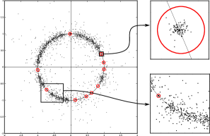
This characteristic of the true poles is a key point on which our method is based: after the computation of $\nu>n$ generalized eigenvalues $\lambda_{i}$, we discard the unstable ones and focus on the stable ones. We now describe in more detail the precise influence of noise in the data $\phi_{j}$ on the $\lambda_{i}$.

2.3 Sensitivity to noise

The exponential analysis of $\phi(t)$, being an inverse problem, is known to be sensitive to noise. Here we briefly recall what is known and in the next section we explain how the new method is able to deal with certain outliers on the one hand and normally distributed noise on the other.

In [24] the authors explain that the roundoff errors in the computation of the generalized eigenvalues are amplified by mainly three sources:

• the scaling of the problem (the $\lambda_{i}$ should lie as closely as possible to the complex unit circle),

• the size of the $|\alpha_{i}|$ relative to the noise ($\lambda_{i}$ with smaller amplitude are more challenging to retrieve),

• the relative position of the $\lambda_{i}$ with respect to each other (clustered $\lambda_{i}$ are hard to separate and retrieve individually).

The first problem is addressed in [24] by means of a diagonal preconditioning matrix, and in [25] by using a suitably chosen invertible upper triangular matrix. The second problem can be tackled with the use of linear time invariant filters which preserve model (2). A solution for the third problem is proposed in [11] and accomplishes a redistribution of the $\lambda_{i}$. Our new method is based on this approach. We now briefly recall the basics of the analysis in [25] to understand the effect of noise and how this is related to the method presented in [11].

Let $(\epsilon_{0},\ldots,\epsilon_{2n-1},\ldots,\epsilon_{N-1})$ again denote the noise vector added to the samples $(\phi_{0},\ldots,\phi_{2n-1},$ $\ldots,\phi_{N-1})$. We rewrite the noise terms $\epsilon_{j}$ as $\epsilon_{j}=\epsilon e_{j}$ where the square Hankel matrices ${}^{0}_{1}E_{n}$ and ${}^{1}_{1}E_{n}$ of size $n$, filled as in (4) but now with the $e_{j}$ instead of the $\phi_{j}$, satisfy

$$||{{}^{0}_{1}}E_{n}||_{2}\leq 1,\qquad||{{}^{1}_{1}}E_{n}||_{2}\leq 1.$$

Let $L_{i}(\lambda)$ denote the Lagrange basis polynomial of degree $n-1$ with roots $\lambda_{1},\ldots$, $\lambda_{i-1}$, $\lambda_{i+1}$,$\ldots,\lambda_{n}$ and $L_{i}(\lambda_{i})=1$, so

$$L_{i}(\lambda)=\frac{\prod_{k=1,k\not=i}^{n}(\lambda-\lambda_{k})}{\prod_{k=1,k\not=i}^{n}(\lambda_{i}-\lambda_{k})}.$$

The coefficients of the polynomial $L_{i}(\lambda)$ make up the vector $\ell_{i}$ of size $n$. Then the disposedness $\rho_{i}$ of the generalized eigenvalue $\lambda_{i}(\phi_{0}+\epsilon e_{0},\ldots,\phi_{N-1}+\epsilon e_{N-1})$, as a function of the given $\phi_{j}$ and the noise terms $\epsilon_{j}=\epsilon e_{j}$, is defined by

$$\rho_{i}:=\left|{d\lambda_{i}\over d\epsilon}(0)\right|$$

and satisfies

$$\rho_{i}\leq{|\lambda_{i}|+1\over|\alpha_{i}|}\;||\ell_{i}||_{2}^{2}\;(||{{}_{1}^{1}}H_{n}||_{2}+||{{}_{1}^{0}}H_{n}||_{2}).$$ (8)

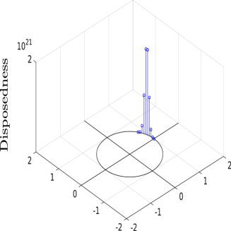
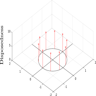
A generalized eigenvalue $\lambda_{i}$ is ill-disposed when $\rho_{i}$ is large. Larger $\rho_{i}$ imply higher susceptibility to noise. Besides the Froissart phenomenon described earlier, the disposedness $\rho_{i}$ of the generalized eigenvalues, or rather its computable upper bound given in (8), is another tool to use when inspecting the $\lambda_{i}$. In Figure 2 we illustrate the relationship between the $\rho_{i}$ and the relative position of the $\lambda_{i}$ with respect to each other: we plot the right hand side of (8) for a toy problem where we choose $\Omega=100,n=10,\alpha_{i}=1,\mu_{i}=\mathrm{i}2\pi(i-1)$. At the left the upper bounds for the values $\rho_{i}$ are plotted at the locations of the generalized eigenvalues $\lambda_{i}=\exp(\mu_{i}\Delta)=\exp(\mu_{i}/\Omega),i=1,\ldots,10$. Now let us change the undersampling parameter $u$ in ${}^{s}_{u}H_{n}$ in (4) and (8) from $u=1$ to $u=10$, which is equivalent to replacing $\Delta$ by $u\Delta$ or replacing $\Omega$ by $\Omega/u$. We recompute the generalized eigenvalues ${}_{u}\lambda_{i}=\exp(\mu_{i}(10\Delta))=\exp(10\mu_{i}/\Omega)$ and the disposedness, which we now denote by ${}_{u}\rho_{i}$. The result, which is shown at the right, changes dramatically, from $O(10^{21})$ to almost $O(10^{1})$.

Figure 2: Ill-disposed ${}_{1}\lambda_{i}=\exp(\mathrm{i}2\pi(i-1)/100)$ at the left and well-disposed ${}_{10}\lambda_{i}=\exp(\mathrm{i}2\pi(i-1)/10)$ at the right, $i=1,\ldots,10$.

Another important tool for inspecting the $\lambda_{i}$ is the Cramèr-Rao lower bound (CRLB) [26, 27]. For any given unbiased estimator of the parameters in (2) and a specific amount and type of noise, the CRLB returns the minimal variance that the estimator suffers. In our case, the estimator is any implementation of Prony’s method and the type of noise is white circular Gaussian noise. The CRLB depends on the number of samples $N$, the variance and type of noise and the set of parameters $|\alpha_{i}|,\arg(\alpha_{i}),\Re(\mu_{i})$ and $\Im(\mu_{i})$. The bound is often used to compare the variance of a specific estimator to this theoretical lower bound. The closer an estimator is to the CRLB, the more efficient it is said to be.

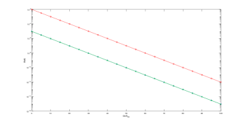
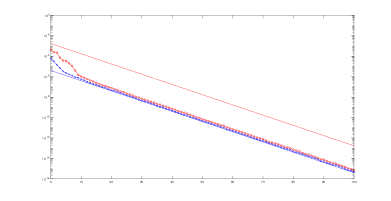
We consider the practical computation of the CRLB provided in [27] and illustrate the relationship between the CRLB and the disposedness $\rho_{i}$ of $\lambda_{i},i=1,\ldots,n$. Take the same toy example and add white circular Gaussian noise of varying signal to noise ratio (SNR). In Figure 3 we graph the root mean square of the vector of CRLB’s for the parameters $\Im(\mu_{i}),i=1,\ldots,10$, and this for decreasing SNR in three different situations:

• $\Delta=1/\Omega,N=200$ samples $\phi_{j}$ (blue triangles),

• $\Delta=10/\Omega,N=200$ samples $\phi_{j}$ (green squares),

• $\Delta=10/\Omega,N=20$ samples $\phi_{j}$ (red circles).

Note that multiplying $\Delta$ by $u=10$ while maintaining $N=200$ implies that the signal is sampled over a larger time interval, while multiplying $\Delta$ by $u=10$ and dividing $N$ by $u=10$ does not enlarge the observation window. So in the first and second case the number of samples is equal while in the first and third case the observation window is equal. Our aim is to get the best of both worlds: while decimation of the signal samples takes you from the CRLB in blue (triangles) to the CRLB in red (circles), we want to recombine separate decimations in order to return from the latter to the former while profiting from some additional features on the way. Decimation significantly diminishes the size of the generalized eigenvalue problems, improves the numerical conditioning, and will automatically return a reliable estimate for the model order $n$. How this can be done is described in Section 4 and illustrated in Figure 18.

Figure 3: Root mean square of the CRLB vector of the $\Im(\mu_{i}),i=1,\ldots,10$, respectively for $\Omega=100,N=200$ (blue), $\Omega=10,N=200$ (green), $\Omega=10,N=20$ (red).

3 Recovering from aliasing after decimation

So we know that choosing $u>1$ may positively impact the disposedness of the $\lambda_{i}$, without negatively impacting the CRLB if the total number of samples can approximately be maintained. Since introducing $u$ impacts $\Delta$ or $\Omega$, aliasing may occur when (3) is violated. We now explain how to deal with this effect: the goal is to enjoy the positive influence of a larger $u$ without suffering the aliasing effect introduced by it.

3.1 Decimation

Instead of using the consecutive set of samples $\phi_{j},j=0,\ldots,2n-1,\ldots N-1$, we consider the decimated set $\phi_{uj}$ which is obtained by considering one sample every $u$ samples, thus sampling $\phi(t)$ at $j(u\Delta)$. The generalized eigenvalue problem

$$({{}^{u}_{u}}H_{n})v=\lambda({{}^{0}_{u}}H_{n})v,$$

leads to a new set of generalized eigenvalues

$${{}_{u}\lambda}_{i}:=\exp(\mu_{i}u\Delta)=\lambda_{i}^{u},\qquad i=1,\ldots,n.$$

From ${{}_{u}\lambda}_{i}$ we cannot directly retrieve $\lambda_{i}$, due to the disruption of (3). We are left with a set of possible values for $\lambda_{i}$ given by

$$U_{i}:=\left\{\exp\left(\mu_{i}\Delta+{2\pi\mathrm{i}\over u}\ell\right),\ell=0,\ldots,u-1\right\}.$$

Despite this, we can already compute the coefficients $\alpha_{i}$ by solving the linear system

$$\phi_{uj}=\sum_{i=1}^{n}\alpha_{i}({{}_{u}\lambda}_{i})^{j},\qquad j=0,\ldots,2n-1,\ldots$$ (9)

Now we consider a shifted set of samples $\phi_{s+uj}$ consisting of at least $n$ samples, for instance at $j=k,\ldots,k+n-1,0\leq k\leq n$, and we choose $s$ coprime with $u$. Since

$$\phi_{s+uj}=\sum_{i=1}^{n}(\alpha_{i}\lambda_{i}^{s})({{}_{u}\lambda}_{i})^{j},\qquad j=k,\ldots,k+n-1,$$ (10)

we denote the coefficient of $({{}_{u}\lambda}_{i})^{j}$ in the shifted sample $\phi_{s+uj}$ by

$${}^{s}\alpha_{i}:=\alpha_{i}\lambda_{i}^{s},\qquad i=1,\ldots,n.$$

We can solve the interpolation conditions (10) for the second set of coefficients ${{}^{s}}{\alpha}_{i}$. Note that the linear systems (10) and (9) have the same Vandermonde structured coefficient matrix, except for the size. This precisely connects the two coefficients $\alpha_{i}$ and ${{}^{s}}\alpha_{i}$, and consequently ${{}^{s}}\lambda_{i}$, to the ${{}_{u}}\lambda_{i}$. From $\alpha_{i}$ and ${{}^{s}}{\alpha}_{i}$ we obtain

$${{}^{s}}{\alpha}_{i}/{\alpha_{i}}=\lambda_{i}^{s},$$

which we can denote by ${{}^{s}\lambda}_{i}$. Due to the same possible disruption of condition (3), ${{}^{s}\lambda}_{i}$ also stands for a set of possible values for $\lambda_{i}$, namely

$$S_{i}:=\left\{\exp\left(\mu_{i}\Delta+{2\pi\mathrm{i}\over s}\ell\right),\ell=0,\ldots,s-1\right\}.$$

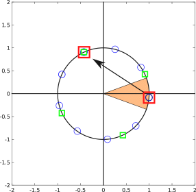
Both sets $U_{i}$ and $S_{i}$ contain the solution $\lambda_{i}$. Since $u$ and $s$ are coprime they share one and only one element which is the non-aliased $\lambda_{i}$ [11]. In Figure 4 we graphically sketch what happens. There $u=9$, the elements in $U_{i}$ are shown using blue circles, $s=4$, the elements in $S_{i}$ are shown using green squares and the arrow points to the unique non-aliased $\lambda_{i}$ in their intersection. The orange portion is the region where the aliased ${{}_{u}\lambda}_{i}$ lies (red square), from which we have to recover the correct $\lambda_{i}$. The aliasing is the consequence of the decimation of the collected samples by a factor $u$.

While in theory $u$ and $s$ may be chosen arbitrarily large, this is not the case in practice, since noise can make it hard to point at the one correct value when a large number of points lie closer together in $U_{i}$ and $S_{i}$. Usually the chosen value of $u$ is larger than that of $s$. Numerical experiments indicate that a smaller $s$ is more important than a smaller $u$: the ${{}_{u}\lambda}_{i}$ values are usually less affected by noise than the ${{}^{s}\lambda}_{i}$ which are obtained as solution of Vandermonde structured linear systems.

Figure 4: Intersection of $U_{i}$ (blue circles, $u=9$) and $S_{i}$ (green squares, $s=4$), relocating the aliased ${{}_{u}\lambda}_{i}$ (red square).

3.2 Recovery

While we know theoretically that $U_{i}$ and $S_{i}$ have only one element in their intersection, we still need to find a way to compute this element in practice. In [11] the following two options are presented. Here we develop a more robust third approach.

An obvious approach is to compute all distances between elements of $U_{i}$ and elements of $S_{i}$ and select the pair that lies closest. This simple approach does not deliver satisfactory results though, because of noise issues. For increasing noise levels, the sets $S_{i}$ may be too perturbed, thus leading to a wrong match of the candidate values for $\lambda_{i}$.

A less obvious approach is to use the Euclidean algorithm and compute two integers $w$ and $r$ satisfying $wu+rs=1$ for the coprime $u$ and $s$. Then $\lambda_{i}$ can be retrieved as

$$({{}_{u}\lambda}_{i})^{w}\;({{}^{s}\lambda}_{i})^{r}=\exp((wu+rs)\mu_{i}\Delta)=\lambda_{i}.$$

The downside of this method is that if $w$ and $r$ are not small, any noise present in ${{}_{u}\lambda}_{i}$ and ${{}^{s}\lambda}_{i}$ is amplified.

We propose to solve a small number of additional systems of the form (10), in order to stabilize the location of the elements in $S_{i}$ before building the distance matrix. We continue the use of shifted samples:

$$\phi_{ms+uj}=\sum_{i=1}^{n}({{}^{ms}\alpha}_{i})\;({{}_{u}\lambda}_{i})^{j},\qquad m=0,\ldots,M-1.$$ (11)

From each shift we compute the coefficients ${{}^{ms}\alpha}_{i}$ and we set up the sequence of values

$$\alpha_{i},{{}^{s}\alpha}_{i},\ldots,{{}^{ms}\alpha}_{i},\ldots,{{}^{(M-1)s}\alpha}_{i},$$

satisfying

$${{}^{ms}\alpha}_{i}=\alpha_{i}({{}^{s}\lambda}_{i})^{m}=\alpha_{i}\exp(\mu_{i}m(s\Delta)),\qquad m=0,\ldots,M-1,$$ (12)

where ${{}^{0}\alpha}_{i}=\alpha_{i}$. So for fixed $i$ the values ${{}^{ms}\alpha}_{i}$ follow the exponential model (12) consisting of only one term. We can therefore use a Prony-like method to extract ${{}^{s}\lambda}_{i}$ in (12) from the values ${{}^{ms}\alpha}_{i}$, just as described in the previous section on basic exponential analysis. This approach stabilizes the location of ${{}^{s}\lambda}_{i}=\lambda_{i}^{s}$ by the use of extra estimates.

At this point we want to point out and stress, that the whole procedure of decimation and recovery can be used on top of any Prony-like method. Retrieving ${{}_{u}\lambda}_{i},{{}^{s}\lambda}_{i}$ or ${{}^{ms}\alpha}_{i}$ for chosen $u$ and $s$ does not require a specific parametric method. In fact, the current procedure offers a way to parallelize existing Prony-like methods, as the decimated signals can be treated independently of each other. In the next section we explain how the combination of the decimated results adds, as one of the features, a validation step to the method, which is mostly lacking in existing Prony-like algorithms.

3.3 Frequency collision

A problem that may occur when decimation causes aliasing, is the possible collision of frequencies. For instance, two distinct eigenvalues $\lambda_{1}$ and $\lambda_{2}$ may be aliased to the same eigenvalue ${{}_{u}\lambda}_{1}={{}_{u}\lambda}_{2}$. However unlikely, we want to discuss how to deal with this situation. We explain the remedy on an example. A fully detailed mathematical analysis of all the eventualities that can occur as a consequence of the decimation, is presented in [11].

Let $\phi(t)$ be specified by $n=2$, $\alpha_{1}=\alpha_{2}=1$, $\mu_{1}=2\pi\mathrm{i}13$, $\mu_{2}=2\pi\mathrm{i}33$. We set $\Omega=100$ and consider one sample $\phi_{j}=\phi(j/\Omega)$ every ten samples ($u=10$) thus changing $\Omega$ to be $10$. Due to aliasing, $\lambda_{1}$ and $\lambda_{2}$ are mapped to another location in the complex plane. In particular, we have

$${{}_{u}\lambda}_{1}={{}_{u}\lambda}_{2}=\exp\left({2\pi\mathrm{i}3\over 10}\right)$$

because

$$\exp\left({2\pi\mathrm{i}33\over 10}\right)=\exp\left({2\pi\mathrm{i}13\over 10}\right)=\exp\left({2\pi\mathrm{i}3\over 10}\right).$$

So in the decimation step (9) Prony’s method retrieves a single frequency with associated coefficient $\alpha_{1}+\alpha_{2}$.

It is however still possible to retrieve the original values $\lambda_{1}$ and $\lambda_{2}$ in the recovery step. As explained, the generalized eigenvalue ${{}_{u}\lambda}_{1}={{}_{u}\lambda}_{2}$ stands for a set of values $U_{1}=U_{2}$ that now contains both the correct $\lambda_{1}$ and $\lambda_{2}$. We choose $s$ coprime with $u$ and compute the values ${{}^{ms}\alpha}_{1}$ (remember that the computed ${{}^{0}\alpha}_{1}=2$ now equals the sum of the true coefficients). Since $s$ is coprime with $u$, no frequency collision occurs in ${{}^{ms}\alpha}_{1}$ which is following the model

$${{}^{ms}\alpha}_{1}=\alpha_{1}\exp(\mu_{1}ms\Delta)+\alpha_{2}\exp(\mu_{2}ms\Delta),\qquad m=0,\ldots,M-1.$$ (13)

So in the analysis of (13) Prony’s method reveals two contributions ${{}^{s}\lambda}_{1}$ and ${{}^{s}\lambda}_{2}$ which bring forth the sets $S_{1}$ and $S_{2}$, respectively containing $\lambda_{1}$ and $\lambda_{2}$. The intersections $U_{1}\cap S_{1}$ and $U_{2}\cap S_{2}=U_{1}\cap S_{2}$ reveal the original $\lambda_{1}$ and $\lambda_{2}$.

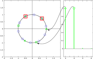
Of course the above can also be applied to the more general case of several collisions in a signal $\phi(t)$ containing more terms. The key element is that the value $M$ in (13) is chosen large enough to allow the identification of all the collided eigenvalues. In particular, $M$ should be at least twice the number of collided eigenvalues. Since this number is unknown, the standard procedure is to take $M$ even and fit the ${{}^{ms}\alpha}_{i}$ with a model of size $M/2$. If less than $M/2$ frequencies have collided, then some of the terms in the expression for ${{}^{ms}\alpha}_{i}$ model the noise and can easily be discarded, as explained in Section 2. We show a typical situation in Figure 5, which applies to the $n=2$ example above: the set $U_{1}=U_{2}$ is depicted using blue circles ($u=10$) and the sets $S_{1}$ and $S_{2}$ using green triangles and squares respectively ($s=3$). We choose $M=8$. The intersections $U_{1}\cap S_{1}$ and $U_{2}\cap S_{2}$ are indicated using red squares.

Figure 5: The $|\alpha_{1}|$ of $\;{{}^{s}\lambda_{1}}$ (green triangle) and $|\alpha_{2}|$ of $\;{{}^{s}\lambda}_{2}$ (green square) at the right ($s=3,M=8$), identifying $U_{1}\cap S_{1}=\{\lambda_{1}\}$ and $U_{2}\cap S_{2}=U_{1}\cap S_{2}=\{\lambda_{2}\}$ from $u=10$ at the left (red squares).

4 Validated exponential analysis

A quite robust Prony-like implementation, which approaches the theoretical CRLB (depicted using blue triangles in Figure 3), is for instance found in [8, 28]. In the sequel we refer to this method as MP, from Matrix Pencil. Our aim now is to maintain as good as the same accuracy, but add the following features to the implementation by making a detour via decimation:

• validation of the output,

• automatic estimation of the model order $n$,

• robustness against some outliers,

• parallelism in the algorithm.

In other words, while the sub-sampling of a signal usually leads to cruder estimates of the already aliased frequencies (upper CRLB curve in Figure 3), the method explained below still achieves the desired CRLB curve (middle curve in Figure 3), while adding a number of desirable features that become available through the technique described in Section 3.

Given a fixed undersampling parameter $u$, we can consider $u$ decimated sample sets $\Phi_{k},k=0,\ldots,u-1$, starting respectively at $0,\Delta,\ldots,(u-1)\Delta$. The first set contains $\lfloor N/u\rfloor$ samples and all subsequent sets contain either the same number of samples or one less:

$$\Phi_{k}:=\{\phi_{uj+k}:j=0,\ldots,\min(\lfloor N/u\rfloor,\lfloor(N-k)/u\rfloor)-1\},\quad k=0,\ldots,u-1.$$

From each decimated set $\Phi_{k}$ we extract ${{}_{u}\lambda}_{i},{{}^{s}\lambda}_{i},i=1,\ldots,n$ which should carry a second index $k$ now to indicate from which decimation $\Phi_{k}$ the values were obtained. The same holds for the coefficients $\alpha_{i}$. For the sequel we therefore introduce the notations $({{}_{u}\lambda}_{i,k}),({{}^{s}\lambda}_{i,k}),{{}^{ms}\alpha}_{i,k}$ with obvious meanings. We also introduce

$${{}_{u}L}:=\cup_{i=1,k=0}^{n,u-1}\{{{}_{u}\lambda}_{i,k}\},\qquad{{}^{s}L}:=\cup_{i=1,k=0}^{n,u-1}\{{{}^{s}\lambda}_{i,k}\}.$$

We remark that the index $i$ still runs from 1 to $n$ even if the undersampling has caused collisions. Then some ${{}_{u}\lambda}_{i,k}$ are merely duplicated.

Each dataset $\Phi_{k}$ is now a decimation of the set of samples $\{\phi_{0},$ $\phi_{1},$ $\ldots,$ $\phi_{N-1}\}$. From this section on, each sample $\phi_{j}$ is always perturbed by noise, but we choose to abuse the notation $\phi_{j}$ instead of $\phi_{j}+\epsilon_{j}$ in order to not overload the presentation. Each set $\Phi_{k}$ is subject to an independent realization of the noise because the latter affects each decimated signal in a different and independent way. Thanks to the connection with the theory of Padé approximation and Froissart doublets, we know that the ${{}_{u}\lambda}_{i,k}$ and ${{}^{s}\lambda}_{i,k}$ form clusters in the sets ${{}_{u}L}$ and ${{}^{s}L}$ respectively, around the true ${{}_{u}\lambda}_{i}=\lambda_{i}^{u}$ and ${{}^{s}\lambda}_{i}=\lambda_{i}^{s}$ with $i=1,\ldots,n$. Any generalized eigenvalues retrieved from overestimating the model order $n$ by $\nu>n$, model the noise and are found scattered around the complex unit disk, as explained in Section 2. To detect the clusters in ${{}_{u}L}$ and ${{}^{s}L}$ we propose to use the density based cluster algorithm DBSCAN [29].

DBSCAN requires two additional parameters: the density $\delta$ of the clusters and the minimum number $m_{\delta}$ of required cluster elements. These parameters are chosen in terms of the noise in the signal. Larger values of $\delta$ allow the detection of wider clusters, which is useful in case of a higher noise level. Smaller values of $\delta$ allow to detect denser clusters, which appear in case of very stable estimates ${{}_{u}\lambda}_{i,k}$ or low levels of noise. A value for $m_{\delta}$ smaller than $u$ allows to discard bogus estimates appearing as a consequence of, for instance, an outlier in the data. When $m_{\delta}$ is set equal to $u$, each ${{}_{u}\lambda}_{i}$ needs to be confirmed by all the decimated analyses. Remember that, through the coefficient matrix shared between (9) and (10), each element from ${{}^{s}L}$ is connected to an element in ${{}_{u}L}$. So any cluster detected in ${{}^{s}L}$ is tied to a set of elements from ${{}_{u}L}$ of the same size. We also point out that the introduction of decimation reduces the complexity of the numerical algorithm and parallelizes the exponential analysis. Instead of solving a single large structured generalized eigenvalue problem, one is facing $u$ much smaller structured generalized eigenvalue problems, which makes a big difference even when solved sequentially. Each $\Phi_{k}$ is analyzed independently and the computation of the ${{}_{u}\lambda}_{i,k}$ and ${{}^{s}\lambda}_{i,k}$ does not need data from other decimations. All the results are collected after the individual runs and then passed to the cluster analysis.

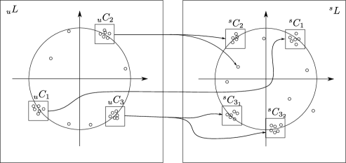
Essentially three different DBSCAN scenario’s can occur, as sketched in Figure 6: at the left we find the result of running DBSCAN on the set ${{}_{u}L}$ and at the right the result on the set ${{}^{s}L}$.

4.1 Standard scenario

A cluster ${{}_{u}C}_{1}$ is detected in the set ${{}_{u}L}$ and its center of gravity can serve as an estimate of one of the $\lambda_{i}^{u}$. The elements ${{}^{s}\lambda}_{i,k}$ tied to the generalized eigenvalues ${{}_{u}\lambda}_{i,k}\in{{}_{u}C}_{1}$ also form a cluster, which we denote by ${{}^{s}C}_{1}$. Its center of gravity then returns an estimate of $\lambda_{i}^{s}$. From both centers of gravity a reliable estimate of $\lambda_{i}$ can be extracted as described in Section 3.2. With each identified $\lambda_{i}$ we can return a list of extra informational items:

• the number of elements validating ${{}_{u}\lambda}_{i}$ in the ${{}_{u}L}$ cluster,

• the number of elements validating ${{}^{s}\lambda_{i}}$ in the ${{}^{s}L}$ cluster,

• the actual radius of the ${{}_{u}L}$ cluster around ${{}_{u}\lambda}_{i}$,

• the actual radius of the ${{}^{s}L}$ cluster around ${{}^{s}\lambda}_{i}$,

The cardinality of the ${{}_{u}L}$ cluster ${{}_{u}C}_{1}$, which indicates how many decimated analyses succeeded in retrieving $\lambda_{i}^{u}$, indicates the level of validation of the retrieved $\lambda_{i}$, while that of the ${{}^{s}L}$ cluster ${{}^{s}C}_{1}$, in combination with its radius, reflects the correct or poor resolution from the aliasing. The radius of ${{}_{u}C}_{1}$ on the one hand and of ${{}^{s}C}_{1}$ on the other, is a measure of the perturbation suffered by respectively $\lambda_{i}^{u}$ and $\lambda_{i}^{s}$. Clusters with few elements and large radii indicate that the conclusion may be wrong because of the inherent noise. The total number of clusters detected in ${{}_{u}L}$ and validated in ${{}^{s}L}$, is automatically a good estimate of the model order $n$, as pictured in Figure 6.

4.2 Outlier scenario

It may happen that not all elements ${{}^{s}\lambda}_{i,k}$ tied to the ${{}_{u}\lambda}_{i,k}$ in a detected cluster ${{}_{u}C}_{2}$ belong to a cluster ${{}^{s}C}_{2}$. In that case the remote elements in ${{}^{s}L}$ are discarded and an estimate for ${{}^{s}\lambda}_{i}=\lambda_{i}^{s}$ is still the center of gravity of ${{}^{s}C}_{2}$. Here the number of decimated analyses validating $\lambda_{i}$ is different in ${{}_{u}L}$ and ${{}^{s}L}$.

4.3 Collision scenario

In cluster ${{}_{u}C}_{3}$ of Figure 6 a collision is involved. As in (13) and pictured in Figure 5, the ${{}^{ms}\alpha}_{i,k}$ have identified more than one exponential contribution. In ${{}^{s}L}$ different clusters of the ${{}^{s}\lambda}_{i,k}$ tied to the ${{}_{u}\lambda}_{i,k}$ in ${{}_{u}C}_{3}$ are identified instead of one large cluster. The centers of gravity of these individual clusters serve to identify the different generalized eigenvalues that have collided ${{}_{u}C}_{3}$ as a consequence of the aliasing.

Figure 6: The cluster algorithm as explained in Section 4, with the set ${{}_{u}L}$ at the left and the set ${{}^{s}L}$ at the right.

4.4 On the choice of $\delta$ and $m_{\delta}$

At first sight, one may think that the new method, which now returns the sparsity $n$ of $\phi(t)$ automatically by counting the number of detected and validated clusters, heavily depends on a proper choice of the new parameters $\delta$ and $m_{\delta}$. This is actually not the case, because usually multiple DBSCAN runs are performed, starting with a high validation rate $m_{\delta}\leq u$ and a small radius $\delta$, relaxing both gradually by decreasing $m_{\delta}$ and increasing $\delta$, until the clusters detected in ${{}_{u}L}$ are not validated anymore by a cluster in ${{}^{s}L}$. Starting with more demanding validation parameters identifies the most stable results first and then explores the remaining results in a less strict way. We often choose $m_{\delta}$ in the range $[0.75,0.95]\times u$. As the ${{}_{u}\lambda}_{i}$ values are usually less affected by noise than the ${{}^{s}\lambda}_{i}$ which are obtained as solution of Vandermonde structured linear systems, the clusters in ${}_{u}L$ are generally denser than the ones in ${}^{s}L$. So, in addition to the above, one should relax both $m_{\delta}$ and $\delta$ a bit when moving with DBSCAN from ${}_{u}L$ to ${}^{s}L$.

All the above is best illustrated with an example of an extreme case. We take $n=2,\nu=3$ and $u=7,s=9$. We construct the illustration so as to generate difficult and large clusters, even exceeding the maximal theoretical cluster size $u$ of the decimation, by considering many different noise realizations. We aim for one dense and one diffuse cluster, with both getting entangled as a consequence of their size and characteristic, and many unwanted Froissart doublet poles on top. Consider for $j=0,\ldots,13$ and $\Delta=0.6028$,

$$\phi(t_{s+ju})=\alpha_{1}\exp(-\mathrm{i}3.3576922(s+ju)\Delta)+\alpha_{2}\exp(\mathrm{i}2.5206137(s+ju)\Delta),$$ (14)

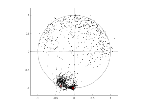
perturbed by white Gaussian noise with SNR $=20$ dB. Such a collection of $2\times 14$ samples (for $u=7,s=0$ and $u=7,s=9$) can result from the described decimation technique. For the time being, let us call one such collection a snaphot and let us generate 512 snapshots by changing the noise realization in the snapshot. From snapshot to snapshot the frequencies $\mu_{i}$ in (2) remain unaltered. So the generalized eigenvalues ${}_{u}\lambda_{i}=\exp(\mu_{i}(u\Delta)),i=1,2$ do not change from snapshot to snapshot. And neither do the values ${}^{s}\lambda_{i}=\exp(\mu_{i}(s\Delta)),i=1,2$. In Figure 7 one finds the $512\times\nu=1526$ values ${}_{u}\lambda_{i}$ at the left and the same number of values ${}^{s}\lambda_{i}$ at the right. One clearly observes two clusters in each of ${}_{u}L$ and ${}^{s}L$, as should be the case since $n=2$, one denser and one more diffuse cluster, and a lot of scattered results coming from the fact that $n$ is overestimated by $\nu>n$.

Figure 7: Joint ${}_{7}\lambda_{1,2}$ (at the left) and ${}^{9}\lambda_{1,2}$ (at the right) of (14) for all noise realizations.

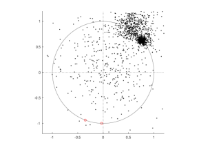
We now discuss the cluster detection in ${}_{u}L$ in more detail. Remember that the process in ${}^{s}L$ is completely analogous, only with somewhat more relaxed values for $m_{\delta}$ and $\delta$.

When running DBSCAN a single time, either with a small density $\delta$ or a larger one, the correct result is not retrieved. When $\delta$ is small (take $\delta=0.1$), then only the denser cluster is revealed. When $\delta$ is larger, large enough to go beyond the dense cluster (take $\delta=0.2$), then both clusters are joined into one. In both tries, we choose $m_{\delta}=\lceil 0.85\times 512\rceil=436$.

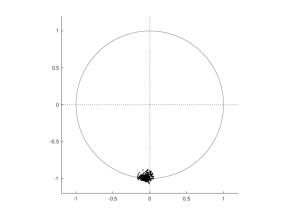
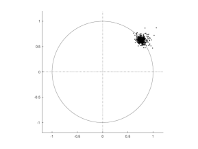
When using multiple DBSCAN runs, as explained above, the correct result is revealed. Let us still fix $m_{\delta}=436$, but now vary $\delta$ from small to large as $\delta=0.08\ell,\ell=1,\ldots,5$. With $\delta=0.08$ a first cluster is detected in respectively ${}_{u}L$ and ${}^{s}L$, as shown in Figure 8. After detecting this cluster, the concerned points are removed from the cluster analysis. With $\delta=0.24$ a second cluster is detected in respectively ${}_{u}L$ and ${}^{s}L$ and shown in Figure 9. For $\delta=0.16$ no cluster is found. Actually, from $\delta=0.32$ on, up to $\delta=0.80$ no clusters are identified anymore.

Figure 8: Dense cluster for (14) retrieved in ${}_{u}L$ (left) and ${}^{s}L$ (right).

Figure 9: Diffuse cluster for (14) retrieved in ${}_{u}L$ (left) and ${}^{s}L$ (right).

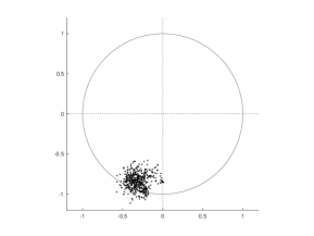
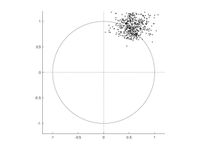
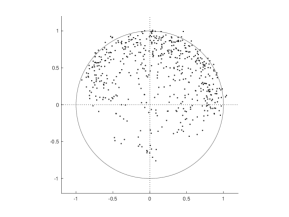
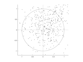
When continuing the search with $\delta=0.88$ then a very diffuse cluster of 504 elements pops up again in ${}_{u}L$ (see Figure 10 left) but without confirmation by the clustering of the associated points in ${}^{s}L$ (see Figure 10 right). So at this point, the search for clusters has definitely been taken across reasonable values for $\delta$.

Figure 10: Candidate cluster for (14) retrieved in ${}_{u}L$ (left) without associated cluster in ${}^{s}L$ (right).

Another unrelated consideration that must be made with respect to $m_{\delta}$ is the following. Let us denote $m_{\delta}=p\times u,0<p\leq 1$, where $p$ denotes the percentage of the maximal cluster size $u$ that we minimally require for the cluster cardinality. If the set of $N$ signal samples still contains some, say $\ell$, remaining outliers, despite an outlier filtering step which is the initial preparation step prior to any further analysis of the data, then in the worst case only $u-\ell$ elements can be found in each cluster, and it is easily understood that we do not want $u-\ell$ to be insignificantly small. This happens when each outlier contaminates a different subset $\Phi_{k},k=1,\ldots,u$ of the decimation. So we have the constraint $m_{\delta}\leq u-\ell$ or $\ell\leq(1-p)u$, which is in practice too strict, but presents at least another indication of the connection between $m_{\delta}$ and the quality of the data set. The strict bound on $\ell$ actually guarantees that the decimation and clustering will not be bothered by the outliers. When the strict bound is violated, the success of the method depends on the location of the outliers and the probability that sufficient subsets $\Phi_{k},k=0,\ldots,u-1$ in the decimation are outlier free.

5 Numerical illustration

At this moment we introduce the acronym VEXPA for the new procedure that validates an exponential analysis carried out by a Prony-like method applied to each of the decimated signals. In order to see the proposed method at work, we present the results of two experiments, with the main aim to illustrate the extra features listed in Section 4, which can now be added to whatever underlying Prony-like method used for each separate decimated analysis. For our experiments we use MP as the underlying method of choice to compute the aliased results ${{}_{u}\lambda}_{i,k}$ modelling the data $\Phi_{k}$ and to compute the recovery values ${{}^{s}\lambda}_{i,k}$ modelling the ${{}^{ms}\alpha}_{i,k}$. We then compare the VEXPA results to those of either the stand-alone MP method or another popular Prony-like alternative [9] and the atomic norm minimisation (ANM) [4].

All experiments are reproducible by downloading the matlab code and data used in 5.1 and 5.2 from cma.uantwerpen.be/publications.

5.1 Outlier experiment

As discussed earlier, the cluster analysis makes the underlying exponential analysis algorithm more robust with respect to outliers that may have escaped an outlier filtering step. In general, it is known that neither methods of the Prony family nor basic implementations of ANM can deal properly with impulsive noise or spikes in the data [30].

In Section 4.4 the relation $\ell\leq u-m_{\delta}$, between the undersampling factor $u$ of the decimation, the number of outliers $\ell$ in the data and the choice for the validation number $m_{\delta}$, is explained. We illustrate all this in the following example.

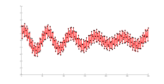
Consider $\phi(t)$ defined by the parameters $|\alpha_{i}|$, $\arg(\alpha_{i})$, $\Im(\mu_{i})$, $\Re(\mu_{i})$, $i=1,2,3$ listed in Table 1. The total number of samples is $N=300$ and the bandwidth is $\Omega=1000$. White circular Gaussian noise with SNR $=30$ dB is added as well as some outliers. We show the real part of the signal and disturb with real-valued outliers. We notice no difference in the conclusions whether the outliers are real, imaginary or complex. The following conclusions hold throughout.

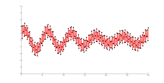
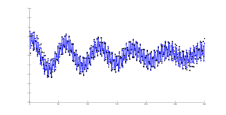
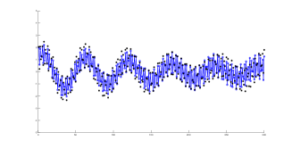
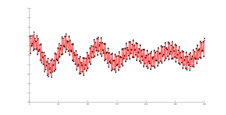
To establish some reference material, we first analyze the by noise corrupted but outlier free signal. On the one hand, we use a TLS-Prony method [9] which takes the numerical rank of the Hankel matrix ${}_{1}^{0}H_{(N-\nu)\times\nu}$ as a guess for the sparsity $n$. On the other hand, we compare this result to the output delivered by VEXPA with underlying the Prony-like algorithm MP [8]. Both methods recover the three terms and perform equally well. The singular value plot of the Hankel matrix ${}_{1}^{0}H_{200\times 100}$ used by the TLS-Prony method, is given at the left in Figure 12. The root-mean-square errors are around 0.008 and the reconstructions are shown in Figure 11, with the data in black, the TLS-Prony result in blue at the left and the VEXPA result in red at the right.

Figure 11: Outlier free reference with original data (in black), TLS-Prony reconstruction (left, in blue) and VEXPA reconstruction (right, in red).

Figure 12: Numerical rank computation of ${}_{1}^{0}H_{200\times 100}$, from outlier free data (left) and single outlier data (right).

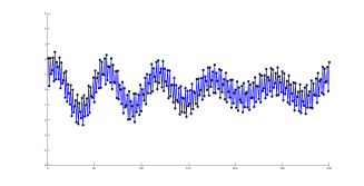
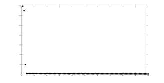
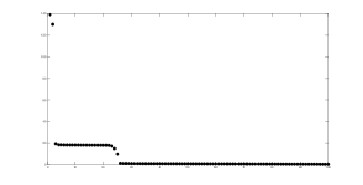
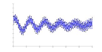
Already from one randomly placed outlier, we see that the RMSE of the result delivered by VEXPA on top of an exponential analysis method is generally less than that of the stand-alone method. Let us, for instance, subtract 18 from sample number 21. The singular value plot for the Hankel matrix constructed with the data containing one outlier, is given in Figure 12 at the right. Thresholding of the singular values of ${{}_{1}^{0}}H_{200\times 100}$ very obviously suggests to truncate all but two terms in the TLS step, although $n=3$ (opting for $n=25$ instead, results in modelling the noise and outlier as well as the signal). So the third term is fully buried by the outlier in the signal and we see this happen in all the subsequent outlier tests on this signal. All subsequent singular value plots look similar and are but slight variations of this one. The reconstruction of the signal using the two recovered terms is shown in Figure 13, at the left in blue. The reconstruction recovers quite well from the outliers, but towards the end of the observation window, the signal deviates more from the original. The RMSE, computed with respect to the noisefree and outlier free signal, is 0.2912.

Figure 13: Outlier experiment with original data (in black), TLS-Prony reconstruction (left, in blue) and VEXPA reconstruction (right, in red).

$|\alpha_{i}|$	$\arg(\alpha_{i})$	$\Im(\mu_{i})$	$\Re(\mu_{i})$
1	0.3342	$2\pi 417.764$	-0.1
1	0.8084	$-2\pi 17.4$	0
0.5	0.5880	$-2\pi 19.5$	0

Table 1: Section 5.1 experiment with $n=3$ and $N=300$.

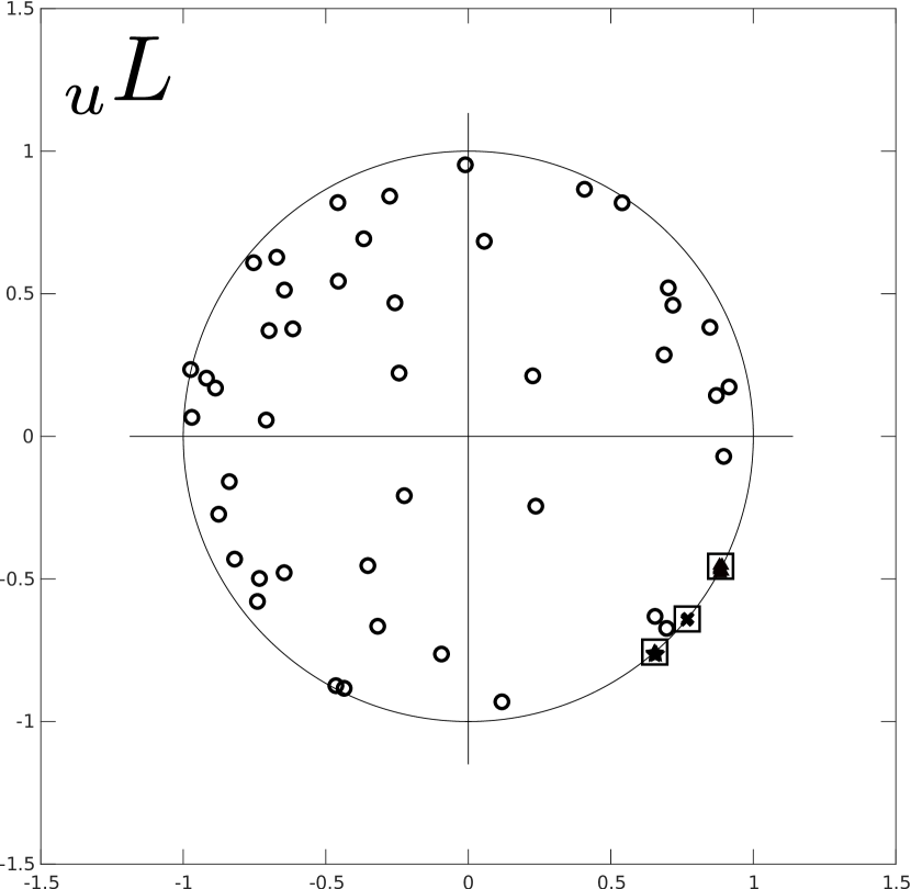
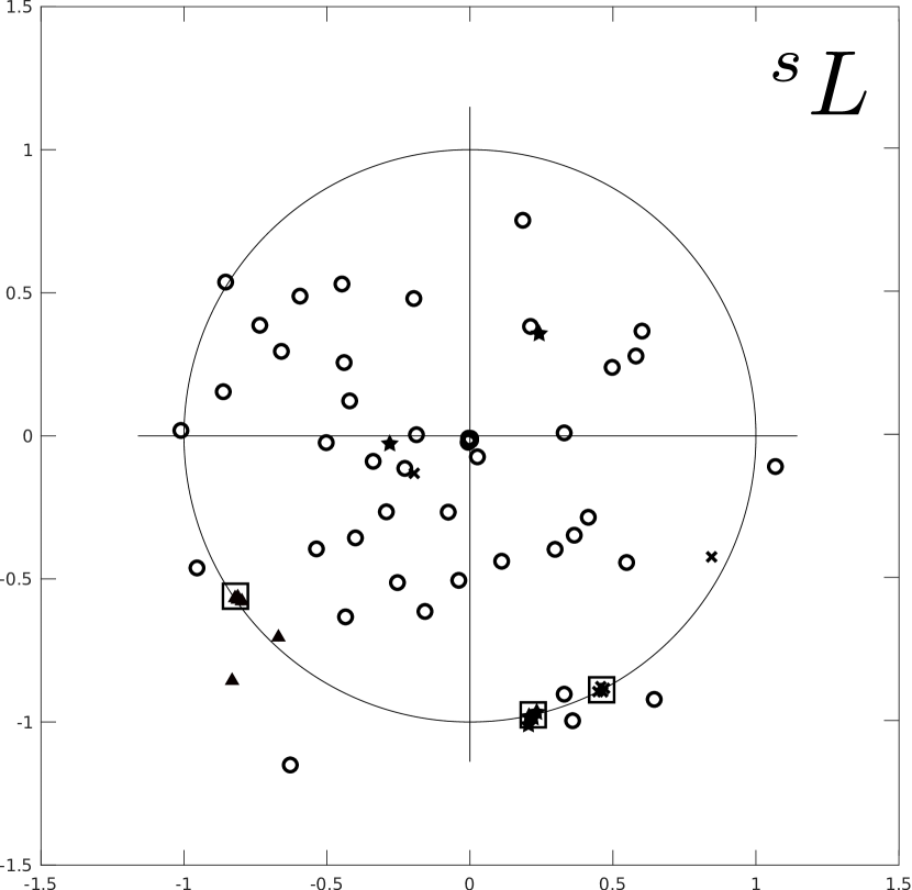
Next, the original signal is analyzed using VEXPA with underlying the Prony-like algorithm MP without SVD thresholding, without a guess for $n$. For VEXPA we take $u=7$ and $s=11$. So each $\Phi_{k}$ contains 42 or 41 samples. The decimation $\Phi_{0}$ contains the outlier. So we can expect to find clusters of 6 elements in ${{}_{u}L}$ instead of 7. Let us choose $m_{\delta}=5$. We identify the ${{}_{u}L}$ clusters using increasing $\delta$-values, say $\delta=0.01,0.03,0.05$, to isolate the most stable results first. In Figure 14 we show the results of the DBSCAN cluster analysis on ${{}_{u}L}$ and ${{}^{s}L}$. The VEXPA add-on clearly identifies $n=3$ exponential terms in the signal and reconstructs the signal quite reliably over the whole time interval. The signal reconstructed from the VEXPA output is depicted in Figure 13, at the right in red. The RMSE is now 0.1164.

Figure 14: Cluster detection in ${{}_{u}L}$ (left) and ${{}^{s}L}$ (right) for the outlier experiment.

Very similar results are found with somewhat more outliers. The bound $\ell\leq u-m_{\delta}$ for the worst case, where each outlier disturbs a different subset $\Phi_{k}$, is known to be too strict. But remember that we assume to be dealing with only a few outliers that may have escaped a filtering step. We now illustrate the capabilities of the new method in three different experiments, all starting from the same signal and noise level:

• some statistical information on the RMSE in case of $\ell=2$ outliers, which fits the constraint $\ell\leq u-m_{\delta}$ when $u=7,m_{\delta}=5$,

• a more specific case belonging to these statistical data, where two outliers are located in each other’s vicinity,

• a typical situation where $\ell=5$ outliers are randomly placed, in this case fortunately without affecting all $\Phi_{k}$.

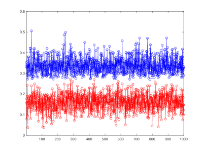
For the statistics, we add randomly chosen outliers belonging to the set $[-25,-15]\cup[15,25]$ to two randomly selected sample numbers between 0 and 299. We do not change the noise, so that the effect that we observe on the computation, compared to Figure 11 with reference RMSE values around 0.008, solely comes from the outliers. The experiment is repeated 1000 times. In Figure 15 we plot the 1000 RMSE of the TLS-Prony result versus that of the VEXPA result.

Figure 15: RMSE of 1000 runs of TLS-Prony (blue, top) versus VEXPA (red, bottom) with 2 outliers randomly placed among the 300 samples.

To illustrate the effect of 2 nearby outliers, we add respectively $-18$ and 24 to the sample numbers 21 and 25. Again the result is very similar. The TLS-Prony reconstruction with 2 terms is shown at the left in blue (see Figure 16) with RMSE $=0.3241$. The VEXPA reconstruction using 3 terms is shown at the right in red (see Figure 16) with RMSE $=0.1393$.

To create 5 outliers we, for instance, respectively add $-18,24,17,-13,20$ to the sample numbers 21, 25, 134, 188, 258. The TLS-Prony method again suggests very obviously to use two terms for the reconstruction (see Figure 17 at the left in blue) with a RMSE $=0.3320$. The VEXPA method with the same parameters for $\delta$ and $m_{\delta}$ reconstructs three terms (see Figure 17 at the right in red) with a RMSE $=0.1390$.

Figure 16: Outlier experiment with 2 outliers placed close to one another.

Figure 17: Outlier experiment with 5 outliers distributed over the signal.

How has the computation of the $\alpha_{i}$ profited from the cluster analysis as well? Since the clusters in ${{}_{u}L}$ consist of 5, 6 or 7 elements, we can deduce precisely which subset(s) $\Phi_{k}$ did not contribute to the validation and so we can omit all data points from such subset(s) in the linear system delivering the parameters $\alpha_{i}$. So the computation of the $\alpha_{i}$ starts from outlier filtered data.

5.2 High noise experiment

For our second experiment we consider a signal $\phi(t)$ defined by the parameters $|\alpha_{i}|,\arg(\alpha_{i}),\Im(\mu_{i}),\Re(\mu_{i}),i=1,\ldots,12$ in Table 2. The total number of samples is again $N=300$, but now with $\Omega=100$. We perturb the samples with white circular Gaussian noise of increasing SNR. The perturbed signal is then analysed using MP (with the added information that $n=12$) on the one hand and VEXPA (on top of MP without the added information that $n=12$) on the other. For the latter we choose $u=7$ and $s=6$. We pass the correct model order $n$ only to MP. The new VEXPA add-on detects it automatically (for ${{}_{u}}L$ and ${{}^{s}}L$ we respectively take $m_{\delta}=6$ and 4, and we choose $\delta=0.1$ twice). For each SNR this experiment is repeated 500 times. The exponential analysis using MP is fed a $200\times 100$ generalized eigenvalue problem which is being reduced to $n=12$ columns after performing an SVD step. On the other hand, each individual decimation solves a $27\times 15$ (or $26\times 15$) generalized eigenvalue problem and afterwards a cluster analysis is performed on the combined outputs of the $u=7$ decimations.

Up to SNR $=10$ dB both MP and VEXPA closely approach the desired CRLB, as can be seen from Figure 18, where we show the CRLB for both $\Omega=100,N=300$ (in blue) and $\Omega=100/7,N=42$ (in red), as in Figure 3. Remember that for each decimation VEXPA is acually departing from the latter situation. But after combining the different decimation results, and effectively also using all the samples, the variance favourably compares to the CRLB. In the meantime, several extra’s have been picked up:

• As a consequence of the decimation, the computational complexity is greatly reduced because of the smaller independent generalized eigenvalue problems.

• Hence the numerical conditioning is improved and the analysis is parallellizable.

• In addition, as already mentioned, the model order $n$ is an automatic byproduct of the cluster analysis.

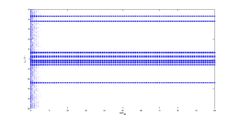
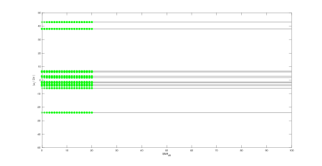
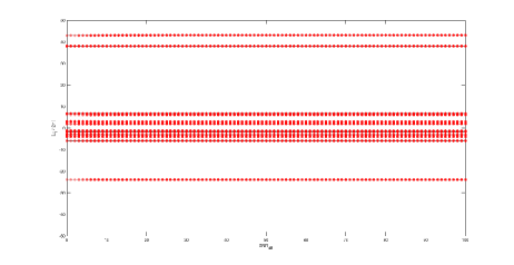
Remains to discuss the gain in reliability. While Figure 18 on the comparison to the CRLB is most interesting in the SNR interval $[10,100]$, the issue of reliability becomes more fascinating for SNR values less than 10. Since the signal is an undamped one, it can also be unravelled using the ANM implementation in [4]. Despite the fact that this implementation enjoys an improved computational complexity of $O(N^{2})$ per iteration step (maximum of 2000 iterations), it takes several hundred times longer per execution than either MP or VEXPA. Therefore the method is only executed 100 times per SNR and this for the more interesting interval of SNR values from 0 to 20. The results of all runs, either 500 or 100, are superimposed in Figure 19: we show all retrieved $\Im(\mu_{i})$-values for MP (top), ANM (middle) and VEXPA (bottom).

For higher noise levels (smaller SNR) the stand-alone MP method returns unreliable results, while the VEXPA method implemented on top of MP detects when the signal is heavily perturbed, namely when fewer computed results are validated in the cluster analysis. So VEXPA, in its standard implementation, does not return unreliable $\lambda_{i}$ output. When none of the results can be validated, then VEXPA does not return $\lambda_{i}$ values at all. Such type of reliability is also offered by ANM, as can be seen in the middle graph: the retrieved frequencies are mostly correct, although some may be missing in case of really small SNR. While the faster exponential analysis methods of the Prony family traditionally suffer from an increased sensitivity to noise (see the top graph on the stand-alone MP results), VEXPA adds as good as the reliability that is normally offered by methods such as ANM (see the middle graph of Figure 19), which can however be prohibitively slow. In addition, we point out that VEXPA can easily be used on damped signals for which the ANM algorithm does not qualify.

Figure 18: Variance of MP (blue) and VEXPA (red), compared to the Cramer-Rao lower bounds obtained as in Figure 3.

Figure 19: Retrieved $\Im(\mu_{i})$ by MP (top, blue), ANM (middle, green) and VEXPA (bottom, red).

$|\alpha_{i}|$	$\arg(\alpha_{i})$	$\Im(\mu_{i})$	$\Re(\mu_{i})$
1	0	$-2\pi 5.93$	0
2	$\pi$	$-2\pi 4.05$	0
2	$\pi/4$	$-2\pi 3.10$	0
2	$\pi/8$	$-2\pi 1.82$	0
2	$3\pi/4$	$-2\pi 1.31$	0
1	$\pi/10$	$2\pi 1.90$	0
3	$-\pi$	$2\pi 2.97$	0
1.5	$-7\pi/8$	$2\pi 6.05$	0
2	0	$2\pi 6.67$	0
3	$-78\pi/100$	$2\pi 38$	0
1	0	$2\pi 43$	0
1	$\pi/5$	$-2\pi 24$	0

Table 2: Section 5.2 experiment with $n=12$ and $N=300$.

6 Conclusion

Exponential analysis methods of the Prony type are more sensitive to noise. We offer an add-on technique that reconditions the problem statement and stabilizes and validates the computed results. As we illustrate in the numerical examples the algorithm works very well. In addition, the method estimates the model order while performing the validation analysis. The approach is highly suited for parallelization and hence further improves the running time of the underlying Prony-like exponential analysis, while offering a reliability comparable to that of the much more computationally intensive atomic norm minimization implementations.

References

- [1] H. Nyquist, Certain topics in telegraph transmission theory, Trans. Am. Inst. Electr. Eng. 47 (2) (1928) 617–644. doi:10.1109/T-AIEE.1928.5055024.
- [2] C. E. Shannon, Communication in the presence of noise, Proc. IRE 37 (1949) 10–21.
- [3] B. N. Bhaskar, G. Tang, B. Recht, Atomic norm denoising with applications to line spectral estimation, IEEE Transactions on Signal Processing 61 (23) (2013) 5987–5999. doi:10.1109/TSP.2013.2273443.
- [4] T. L. Hansen, T. L. Jensen, A fast interior-point method for atomic norm soft thresholding, Signal Processing 165 (2019) 7 – 19. doi:10.1016/j.sigpro.2019.06.023.
- [5] R. de Prony, Essai expérimental et analytique sur les lois de la dilatabilité des fluides élastiques et sur celles de la force expansive de la vapeur de l’eau et de la vapeur de l’alkool, à différentes températures, J. Ec. Poly. 1 (1795) 24–76.
- [6] E. Kaltofen, W.-s. Lee, Early termination in sparse interpolation algorithms, J. Symbolic Comput. 36 (3-4) (2003) 365–400. doi:10.1016/S0747-7171(03)00088-9.
- [7] R. Roy, T. Kailath, ESPRIT-estimation of signal parameters via rotational invariance techniques, IEEE Trans. Acoust., Speech, Signal Process. 37 (7) (1989) 984–995. doi:10.1109/29.32276.
- [8] Y. Hua, T. K. Sarkar, Matrix pencil method for estimating parameters of exponentially damped/undamped sinusoids in noise, IEEE Trans. Acoust., Speech, Signal Process. 38 (1990) 814–824. doi:10.1109/29.56027.
- [9] W. M. Steedly, C.-H. J. Ying, R. L. Moses, Statistical analysis of TLS-based Prony techniques, Automatica 30 (1) (1994) 115–129, special issue on statistical signal processing and control. doi:10.1016/0005-1098(94)90232-1.
- [10] D. Chu, G. H. Golub, On a generalized eigenvalue problem for nonsquare pencils, SIAM J. Matrix Anal. Appl. 28 (3) (2006) 770–787. doi:10.1137/050628258.
- [11] A. Cuyt, W.-s. Lee, How to get high resolution results from sparse and coarsely sampled data, Appl. Comput. Harmon. Anal. 48 (3) (2020) 1066–1087. doi:10.1016/j.acha.2018.10.001.
- [12] P. Henrici, Applied and computational complex analysis I, John Wiley & Sons, New York, 1974.
- [13] A. Cuyt, M. Tsai, M. Verhoye, W.-s. Lee, Faint and clustered components in exponential analysis, Appl. Math. Comput. 327 (2018) 93–103.
- [14] L. Weiss, R. McDonough, Prony’s method, -transforms, and Padé approximation, SIAM Rev. 5 (1963) 145–149.
- [15] Z. Bajzer, A. C. Myers, S. S. Sedarous, F. G. Prendergast, Padé-Laplace method for analysis of fluorescence intensity decay, Biophys. J. 56 (1) (1989) 79–93.
- [16] J. Nuttall, The convergence of Padé approximants of meromorphic functions, J. Math. Anal. Appl. 31 (1970) 147–153. doi:10.1016/0022-247X(70)90126-5.
- [17] C. Pommerenke, Padé approximants and convergence in capacity, J. Math. Anal. Appl. 41 (1973) 775–780. doi:10.1016/0022-247X(73)90248-5.
- [18] J. Gammel, Effect of random errors (noise) in the terms of a power series on the convergence of the Padé approximants, in: P. Graves-Morris (Ed.), Padé approximants, 1972, pp. 132–133.
- [19] D. Bessis, Padé approximations in noise filtering, J. Comput. Appl. Math. 66 (1996) 85–88. doi:10.1016/0377-0427(95)00177-8.
- [20] J. Gilewicz, M. Pindor, Padé approximants and noise: a case of geometric series, J. Comput. Appl. Math. 87 (1997) 199–214. doi:10.1016/S0377-0427(97)00185-4.
- [21] J. Gilewicz, M. Pindor, Padé approximants and noise: rational functions, J. Comput. Appl. Math. 105 (1999) 285–297. doi:10.1016/S0377-0427(99)00041-2.
- [22] P. Barone, On the distribution of poles of Padé approximants to the Z-transform of complex Gaussian white noise, Journal of Approximation Theory 132 (2) (2005) 224 – 240. doi:10.1016/j.jat.2004.10.014.
- [23] L. Perotti, T. Regimbau, D. Vrinceanu, D. Bessis, Identification of gravitational-wave bursts in high noise using Padé filtering, Physical Review D 90 (12) (2014) 124047.
- [24] G. Golub, P. Milanfar, J. Varah, A stable numerical method for inverting shape from moments, SIAM J. Sci. Comput. 21 (1999) 1222–1243.
- [25] B. Beckermann, G. Golub, G. Labahn, On the numerical condition of a generalized Hankel eigenvalue problem, Numer. Math. 106 (1) (2007) 41–68. doi:10.1007/s00211-006-0054-x.
- [26] S. M. Kay, Fundamentals of Statistical Signal Processing: Estimation Theory, Prentice-Hall, Inc., Upper Saddle River, NJ, USA, 1993.
- [27] Y.-X. Yao, S. M. Pandit, Cramer-Rao lower bounds for a damped sinusoidal process, IEEE Trans. Signal Processing 43 (1995) 878–885.
- [28] N. Yilmazer, S. Ari, T. K. Sarkar, Multiple snapshot direct data domain approach and ESPRIT method for direction of arrival estimation, Digital Signal Processing 18 (4) (2008) 561 – 567. doi:10.1016/j.dsp.2007.07.004.
- [29] M. Ester, H.-P. Kriegel, J. Sander, X. Xu, A density-based algorithm for discovering clusters in large spatial databases with noise, in: KDD’96 Proceedings of the Second International Conference on Knowledge Discovery and Data Mining, KDD-96, AAAI Press, 1996, pp. 226–231.
- [30] C. Fernandez-Granda, G. Tang, X. Wang, L. Zheng, Demixing sines and spikes: Robust spectral super-resolution in the presence of outliers, Information and Inference: A Journal of the IMA 7 (1) (2018) 105–168. doi:10.1093/imaiai/iax005.