Effects of spatial curvature and anisotropy on the asymptotic regimes in Einstein-Gauss-Bonnet gravity

Abstract

In this paper we address two important issues which could affect reaching the exponential and Kasner asymptotes in Einstein-Gauss-Bonnet cosmologies – spatial curvature and anisotropy in both three- and extra-dimensional subspaces. In the first part of the paper we consider cosmological evolution of spaces being the product of two isotropic and spatially curved subspaces. It is demonstrated that the dynamics in $D=2$ (the number of extra dimensions) and $D\geqslant 3$ is different. It was already known that for the $\Lambda$-term case there is a regime with “stabilization” of extra dimensions, where the expansion rate of the three-dimensional subspace as well as the scale factor (the “size”) associated with extra dimensions reach constant value. This regime is achieved if the curvature of the extra dimensions is negative. We demonstrate that it take place only if the number of extra dimensions is $D\geqslant 3$. In the second part of the paper we study the influence of initial anisotropy. Our study reveals that the transition from Gauss-Bonnet Kasner regime to anisotropic exponential expansion (with expanding three and contracting extra dimensions) is stable with respect to breaking the symmetry within both three- and extra-dimensional subspaces. However, the details of the dynamics in $D=2$ and $D\geqslant 3$ are different. Combining the two described affects allows us to construct a scenario in $D\geqslant 3$, where isotropisation of outer and inner subspaces is reached dynamically from rather general anisotropic initial conditions.

I Introduction

Extra-dimensional theories have been known Nord1914 even prior to the General Relativity (GR) einst , but relatively known they become after works by Kaluza and Klein KK1 ; KK2 ; KK3 . Since then the extra-dimensional theories evolve a lot but the main motivation behind them remains the same – unification of interactions. Nowadays one of the promising candidate for unified theory is M/string theory.

Presence of the curvature-squared corrections in the Lagrangian of the gravitational counterpart of string theories is one of their distinguishing features. Scherk and Schwarz sch-sch demonstrated the need for the $R^{2}$ and $R_{\mu\nu}R^{\mu\nu}$ terms, while later Candelas et al. Candelas_etal proved the same for $R^{\mu\nu\lambda\rho}R_{\mu\nu\lambda\rho}$. Later it was demonstrated zwiebach that the only combination of quadratic terms that leads to a ghost-free nontrivial gravitation interaction is the Gauss-Bonnet (GB) term:

$$L_{GB}=L_{2}=R_{\mu\nu\lambda\rho}R^{\mu\nu\lambda\rho}-4R_{\mu\nu}R^{\mu\nu}+R^{2}.$$

This term, first found by Lanczos Lanczos1 ; Lanczos2 (therefore it is sometimes referred to as the Lanczos term) is an Euler topological invariant in (3+1)-dimensional space-time, but not in (4+1) and higher dimensions. Zumino zumino extended Zwiebach’s result on higher-than-squared curvature terms, supporting the idea that the low-energy limit of the unified theory might have a Lagrangian density as a sum of contributions of different powers of curvature. In this regard the Einstein-Gauss-Bonnet (EGB) gravity could be seen as a subcase of more general Lovelock gravity Lovelock , but in the current paper we restrain ourselves with only quadratic corrections and so to the EGB case.

While considering extra-dimensional theories, regardless of the model, we need to explain where are additional dimensions. Indeed, with our current level of experiments, we clearly sense three spatial dimensions and sense no presence of extra dimensions. The common explanation is that they are “compactified”, meaning that they are so small that we cannot detect them. Perhaps, the simplest class of such theories are the theories with “spontaneous compactification”. Exact solutions of this class have been known for a long time add_1 , but especially relevant for cosmology are those with dynamical size of extra dimensions (see add_4 ; Deruelle2 ; add_10 ; add_8 for different models). Notable recent studies include add13 , where dynamical compactification of the (5+1) Einstein-Gauss-Bonnet model was considered, MO04 ; MO14 , where different metric Ansätze for scale factors corresponding to (3+1)- and extra-dimensional parts were studied and CGP1 ; CGP2 ; CGPT , where we investigated general (e.g., without any Ansatz) scale factors and curved manifolds. Also, apart from cosmology, the recent analysis has focused on properties of black holes in Gauss-Bonnet alpha_12 ; add_rec_1 ; add_rec_2 ; addn_1 ; addn_2 and Lovelock add_rec_3 ; add_rec_4 ; addn_3 ; addn_4 ; addn_4.1 gravities, features of gravitational collapse in these theories addn_5 ; addn_6 ; addn_7 , general features of spherical-symmetric solutions addn_8 , and many others.

When it comes to exact cosmological solutions, two most common Ansatz used for the scale factor are exponential and power law. Exponential solutions represent de Sitter asymptotic stages while power-law – Friedmann-like. Power-law solutions have been analyzed in Deruelle1 ; Deruelle2 and more recently in mpla09 ; prd09 ; Ivashchuk ; prd10 ; grg10 so that by now there is an almost complete description of the solutions of this kind (see also PT for comments regarding physical branches of the power-law solutions). One of the first considerations of the extra-dimensional exponential solutions was done by Ishihara Is86 ; later considerations include KPT , as well as the models with both variable CPT1 and constant CST2 volume; the general scheme for constructing solutions in EGB gravity was developed and generalized for general Lovelock gravity of any order and in any dimensions CPT3 . Also, the stability of the solutions was addressed in my15 (see also iv16 for stability of general exponential solutions in EGB gravity), and it was demonstrated that only a handful of the solutions could be called “stable”, while the most of them are either unstable or have neutral/marginal stability.

If we want to find all possible regimes in EGB cosmology, we need to go beyond an exponential or power-law Ansatz and keep the scale factor generic. We are particularly interested in models that allow dynamical compactification, so that we consider the spatial part as the warped product of a three-dimensional and extra-dimensional parts. In that case the three-dimensional part is “our Universe” and we expect for this part to expand while the extra-dimensional part should be suppressed in size with respect to the three-dimensional one. In CGP1 we demonstrated the there existence of regime when the curvature of the extra dimensions is negative and the Einstein-Gauss-Bonnet theory does not admit a maximally symmetric solution. In this case both the three-dimensional Hubble parameter and the extra-dimensional scale factor asymptotically tend to the constant values. In CGP2 we performed a detailed analysis of the cosmological dynamics in this model with generic couplings. Later in CGPT we studied this model and demonstrated that, with an additional constraint on couplings, Friedmann late-time dynamics in three-dimensional part could be restored.

Recently we have performed full-scale investigation of the spatially-flat cosmological models in EGB gravity with the spatial part being warped product of a three-dimensional and extra-dimensional parts my16a ; my16b ; my17a . In my16a we demonstrated that the vacuum model has two physically viable regimes – first of them is the smooth transition from high-energy GB Kasner to low-energy GR Kasner. This regime appears for $\alpha>0$ at $D=1,\,2$ (the number of extra dimensions) and for $\alpha<0$ at $D\geqslant 2$ (so that at $D=2$ it appears for both signs of $\alpha$). The other viable regime is smooth transition from high-energy GB Kasner to anisotropic exponential regime with expanding three-dimensional section (“our Universe”) and contracting extra dimensions; this regime occurs only for $\alpha>0$ and at $D\geqslant 2$. In my16b ; my17a we considered $\Lambda$-term case and it appears that only realistic regime is the transition from high-energy GB Kasner to anisotropic exponential regime; the low-energy GR Kasner is forbidden in the presence of the $\Lambda$-term so the corresponding transition do not occur. Also, if we consider joint constraints on $(\alpha,\Lambda)$ from our cosmological analysis and a black holes properties, different aspects of AdS/CFT and related theories in the presence of Gauss-Bonnet term (see alpha_01 ; alpha_02 ; alpha_03 ; alpha_04 ; alpha_05 ; alpha_06 ; alpha_07 ; alpha_08 ; add_rec_2 ; add_rec_4 ; dS ), the resulting bounds on $(\alpha,\Lambda)$ are (see my17a for details)

$$\begin{array}[]{l}\alpha>0,\quad D\geqslant 2,\quad\displaystyle\frac{3D^{2}-7D+6}{4D(D-1)}\equiv\eta_{0}\geqslant\alpha\Lambda\geqslant\eta_{2}\equiv-\displaystyle\frac{(D+2)(D+3)(D^{2}+5D+12)}{8(D^{2}+3D+6)^{2}},\end{array}$$ (1)

where $\alpha$ is the Gauss-Bonnet coupling and $D$ is the number of extra dimensions.

The current paper is a natural continuation of our previous research on the properties of cosmological dynamics in EGB gravity. After a thorough investigation of spatially-flat cases in my16a ; my16b ; my17a , it is natural to consider spatially non-flat cases. Indeed, the spatial curvature affects inflation infl1 ; infl2 , so that it could change asymptotic regimes in other high-energy stages of the Universe evolution, and we are considering one of them. We already investigated the cases with negative curvature of the extra dimensions in CGP1 ; CGP2 ; CGPT , but to complete description it is necessary to consider all possible cases. We are going to consider all possible curvature combination to see their influence on the dynamics – we know the regime for the case with both subspaces being spatially flat and will see the change in the dynamics with the curvatures being non-flat. This allows us to find all possible asymptotic regimes in spatially non-flat case; together with the results for the flat case, it will complete this topic.

Another important issue we are going to consider is the anisotropy within subspaces. Indeed, the analysis in my16a ; my16b ; my17a is performed under conjecture that both three- and extra-dimensional subspaces are isotropic. The question is, if the results are stable under small (or not very small) deviations of isotropy of these subspaces. Finally, if we consider both effects, we could build two-steps scheme which allows us to qualitatively describe the dynamical compactification of anisotropic curved space-time.

The structure of the manuscript is as follows: first we write down the equations of motion for the case under consideration. Next, we study the effects of curvature – we add all possible curvature combinations to all known existing flat regimes and describe the changes in the dynamics. After that we draw conclusions for separately vacuum and $\Lambda$-term regimes and describe their differences and generalities. After that we investigate the effects of anisotropy and find stability areas for different cases. Finally, we use both effects to build two-steps scheme which allow us to describe the dynamics of a wide class spatially curved models. In the end, we discuss the results obtained and draw the conclusions.

II Equations of motion

Lovelock gravity Lovelock has the following structure: its Lagrangian is constructed from terms

$$L_{n}=\frac{1}{2^{n}}\delta^{i_{1}i_{2}\dots i_{2n}}_{j_{1}j_{2}\dots j_{2n}}R^{j_{1}j_{2}}_{i_{1}i_{2}}\dots R^{j_{2n-1}j_{2n}}_{i_{2n-1}i_{2n}},$$ (2)

where $\delta^{i_{1}i_{2}\dots i_{2n}}_{j_{1}j_{2}\dots j_{2n}}$ is the generalized Kronecker delta of the order $2n$. One can verify that $L_{n}$ is Euler invariant in $D<2n$ spatial dimensions and so it would not give nontrivial contribution into the equations of motion. So that the Lagrangian density for any given $D$ spatial dimensions is sum of all Lovelock invariants (2) upto $n=\left[\displaystyle\frac{D}{2}\right]$ which give nontrivial contributions into equations of motion:

$${\cal L}=\sqrt{-g}\sum_{n}c_{n}L_{n},$$ (3)

where $g$ is the determinant of metric tensor, $c_{n}$ is a coupling constant of the order of Planck length in $2n$ dimensions and summation over all $n$ in consideration is assumed.

The ansatz for the metric is

$$ds^{2}=-dt^{2}+a(t)^{2}d\Sigma_{(3)}^{2}+b(t)^{2}d\Sigma_{(\mathbf{D})}^{2}\ ,$$ (4)

where $d\Sigma_{(3)}^{2}$ and $d\Sigma_{(\mathbf{D})}^{2}$ stand for the metric of two constant curvature manifolds $\Sigma_{(3)}$ and $\Sigma_{(\mathbf{D})}$. It is worth to point out that even a negative constant curvature space can be compactified by making the quotient of the space by a freely acting discrete subgroup of $O(D,1)$ wolf .

The complete derivation of the equations of motion could be found in our previous papers, dedicated to the description of the particular regime which appears in this model CGP1 ; CGP2 . It is convenient to use the following notation

$$A_{(1)} = \frac{\overset{..}{a}}{a},\ \ \ C=\frac{\overset{.}{a}\overset{.}{b}}{ab},\ \ \ B_{(1)}=\frac{\overset{..}{b}}{b},$$

$$A_{(2)} = \frac{\left[\gamma_{\left(3\right)}+\left(\overset{.}{a}\right)^{2}\right]}{a^{2}},\ \ \ B_{(2)}=\frac{\left[\gamma_{\left(\mathbf{D}\right)}+\left(\overset{.}{b}\right)^{2}\right]}{b^{2}}$$ (5)

and the following rescaling of the coupling constants

$$\alpha=\frac{\left(D+3\right)\left(D+2\right)\left(D+1\right)}{6}c_{0}\ ,\ \ \ \beta=\frac{\left(D+1\right)D\left(D-1\right)}{6}c_{1}\ ,\ \ \ \gamma=\frac{\left(D-1\right)\left(D-2\right)\left(D-3\right)}{6}c_{2}\ .$$ (6)

Then, the equations of motion could be written in the following form:

$$\begin{array}[]{l}\mathcal{E}_{0}=0\Leftrightarrow 0=\alpha+\beta\left(B_{(2)}+\displaystyle\frac{6}{D-1}C+\displaystyle\frac{6}{D\left(D-1\right)}A_{(2)}\right)+\gamma\left(B_{(2)}^{2}+\displaystyle\frac{12A_{(2)}B_{(2)}}{\left(D-2\right)\left(D-3\right)}+\right.\\ \\ \left.+\displaystyle\frac{24C^{2}}{\left(D-2\right)\left(D-3\right)}+\displaystyle\frac{12B_{(2)}C}{\left(D-3\right)}+\displaystyle\frac{24A_{(2)}C}{\left(D-1\right)\left(D-2\right)\left(D-3\right)}\right),\end{array}$$ (7)

$$\mathcal{E}_{i}=0\Leftrightarrow 0=\alpha+\beta\left(B_{(2)}+\frac{4A_{(1)}}{D\left(D-1\right)}+\frac{2B_{(1)}}{D-1}+\frac{2A_{(2)}}{D\left(D-1\right)}+\frac{4C}{\left(D-1\right)}\right)+\gamma\left(B_{(2)}^{2}+\right.$$

$$+\frac{16A_{(1)}C}{\left(D-1\right)\left(D-2\right)\left(D-3\right)}+\frac{8B_{(2)}C}{D-3}++\frac{8A_{(1)}B_{(2)}}{\left(D-2\right)\left(D-3\right)}+\frac{8A_{(2)}B_{(1)}}{\left(D-1\right)\left(D-2\right)\left(D-3\right)}+$$

$$\left.+\frac{16B_{(1)}C}{\left(D-2\right)\left(D-3\right)}+\frac{4B_{(1)}B_{(2)}}{\left(D-3\right)}+\frac{4A_{(2)}B_{(2)}}{\left(D-2\right)\left(D-3\right)}+\frac{8C^{2}}{\left(D-2\right)\left(D-3\right)}\right)\ \ ,$$ (8)

while the equation $\mathcal{E}_{a}=0$ reads

$$\mathcal{E}_{a}=0\Leftrightarrow 0=\frac{D}{\left(D-4\right)}\alpha+\frac{\left(D-2\right)}{\left(D-4\right)}\beta\left(B_{(2)}+\frac{6A_{(1)}}{\left(D-1\right)\left(D-2\right)}+\frac{2B_{(1)}}{D-2}+\frac{6A_{(2)}}{\left(D-1\right)\left(D-2\right)}+\frac{6C}{\left(D-2\right)}\right)+$$

$$+\gamma\left(B_{(2)}^{2}+\frac{48A_{(1)}C}{\left(D-2\right)\left(D-3\right)\left(D-4\right)}+\frac{12B_{(2)}C}{D-4}+\frac{24C^{2}}{\left(D-3\right)\left(D-4\right)}+\right.$$

$$+\frac{12A_{(1)}B_{(2)}}{\left(D-3\right)\left(D-4\right)}+\frac{24A_{(2)}B_{(1)}}{\left(D-2\right)\left(D-3\right)\left(D-4\right)}+\frac{24B_{(1)}C}{\left(D-3\right)\left(D-4\right)}+\frac{4B_{(1)}B_{(2)}}{\left(D-4\right)}+$$

$$\left.+\frac{12A_{(2)}B_{(2)}}{\left(D-3\right)\left(D-4\right)}+\frac{24A_{(2)}C}{\left(D-2\right)\left(D-3\right)\left(D-4\right)}+\frac{24A_{(1)}A_{(2)}}{\left(D-1\right)\left(D-2\right)\left(D-3\right)\left(D-4\right)}\right).$$ (9)

III Influence of curvature

In this section we investigate the impact of the spatial curvature on the cosmological regimes. As a “background” we use the results obtained in my16a ; my16b ; my17a – exact regimes for $\gamma_{\left(3\right)}=\gamma_{\left(\mathbf{D}\right)}\equiv 0$ for both vacuum and $\Lambda$-term cases. As we use them as a “background” solutions, it is worth to quickly describe them all. All solutions found for both vacuum and $\Lambda$-term cases could be splitted into two groups – those with “standard” regimes as both past and future asymptotes and those with nonstandard singularity as one (or both) of the asymptotes. By the “standard” regimes we mean Kasner (generalized power-law) and exponential. In our study me encounter two different Kasner regimes – “classical” GR Kasner regime (with $\sum p_{i}=\sum p_{i}^{2}=1$ where $p_{i}$ is Kasner exponent from the definition of power-law behavior $a_{i}(t)=t^{p_{i}}$), which we denote as $K_{1}$ (as $\sum p_{i}=1)$ and it is low-energy regime; and GB Kasner regime (with $\sum p_{i}=3$), which we denote as $K_{3}$ and it is high-energy regime. For realistic cosmology we should have high-energy regime as past asymptote and low-energy as future, but our investigation demonstrates that potentially both $K_{1}$ and $K_{3}$ could play a role as past and future asymptotes my16a . Also we should note that $K_{1}$ exist only in the vacuum regime, while $K_{3}$ as past asymptotes we encounter in both vacuum and $\Lambda$-term regimes (see my16b for details). The exponential regimes (where scale factors depend upon time exponentially, so Hubble parameters are constant) could be seen in both vacuum and $\Lambda$-term regimes and there are two of them – isotropic and anisotropic ones. The former of them corresponds to the case where all the directions are isotropized and, since we work in the multidimensional case, it does not fit the observations. On contrary, the latter of them have different Hubble parameters for three- and extra-dimensional subspaces. For realistic compactification we demand expansion of the three- and contraction of the extra-dimensional spaces. The exponential solutions are denoted as $E_{iso}$ for isotropic and $E_{3+D}$ for anisotropic, where $D$ is the number of extra dimensions (so that, say, in $D=2$ the anisotropic exponential solution is denoted as $E_{3+2}$).

The second large group are the regimes which have nonstandard singularity as either of the asymptotes or even both of them. The nonstandard singularity is the situation which arises in nonlinear theories and in our particular case it corresponds to the point of the evolution where $\dot{H}$ (the derivative of the Hubble parameter) diverges at the final $H$; we denote it as $nS$. This kind of singularity is “weak” by Tipler’s classification Tipler and is type II in classification by Kitaura and Wheeler KW1 ; KW2 . Our previous research reveals that nonstandard singularity is a wide-spread phenomena in EGB cosmology, for instance, in $(4+1)$-dimensional Bianchi-I vacuum case all the trajectories have $nS$ as either past or future asymptote prd10 . Since a nonstandard singularity means the beginning or end of dynamical evolution, either higher or lower values of $H$ do not reached and so the entire evolution from high to low energies cannot be restored; for this reason we disregard the trajectories with $nS$ in the present paper.

So that the viable (or realistic) regimes are limited to $K_{3}\to K_{1}$ and $K_{3}\to E_{3+D}$ for vacuum case and $K_{3}\to E_{3+D}$ for $\Lambda$-term; these regimes we further investigate in the presence of curvature.

III.1 Vacuum $K_{3}\to K_{1}$ transition with curvature

First we want to investigate the influence of the curvature on the vacuum Kasner transition – transition from Gauss-Bonnet Kasner regime $K_{3}$ to standard GR Kasner $K_{1}$. We add curvature to either and both three- and extra-dimensional manifolds and see the changes in the regimes. We label the cases as $(\gamma_{3},\gamma_{D})$ where $\gamma_{3}$ is the spatial curvature of the three-dimensional manifold and $\gamma_{D}$ – of the extra-dimensional. So that for $(0,0)$ – flat case – we have $K_{3}\to K_{1}$, as reported in my16a . Now if we introduce nonzero curvature, both $(1,0)$ and $(-1,0)$ do not change the regime and it remains $K_{3}\to K_{1}$. So that we can conclude that $\gamma_{3}$ alone do not affect the dynamics. On contrary, $\gamma_{D}$ does – $(0,1)$ has the transition changes to $K_{3}\to K_{3}^{S}$ (finite-time future singularity of the power-law type with $K_{3}$ behavior – analogue of the recollapse from the standard cosmology), while $(0,-1)$ change the transition to $K_{3}\to K_{D}$. This $K_{D}$ is a new but non-viable regime with $p_{3}\to 0$ and $p_{D}\to 1$ – regime with constant-size three dimensions and expanding as power-law extra dimensions, which makes the behavior in the expanding subspace Milne-like, caused by the negative curvature. So that the curvature of the extra dimensions alone makes future asymptotes non-viable. If we include both curvatures, the situation changes as follows: for $(1,1)$ we have $K_{3}\to K_{3}^{S}$; for $(1,-1)$ it is $K_{3}\to K_{D}$; for $(-1,1)$ it is $K_{3}\to K_{3}^{S}$ and finally for $(-1,-1)$ it is $K_{3}\to K_{D+3}^{iso}$.

The described regimes require some explanations. First of all, as we reported in my16a , viable regimes have $p_{a}>0$ and $p_{D}<0$ – indeed, we want expanding three-dimensional space and contracting extra dimensions to achieve compactification. Then, it is clear why $\gamma_{3}$ alone does not change anything – with expanding scale factor, the effect of curvature vanishes. It is also clear why $\gamma_{D}=+1$ makes $K_{3}^{S}$ as future asymptote – positive spatial curvature prevents infinite contracting of the extra dimensions and gives rise to new regime. But the most interesting is the effect of $\gamma_{D}=-1$ – indeed, negative curvature not just stops the contraction of the extra dimensions but starts their expansion, which change the entire dynamics drastically. Now extra-dimensional scale factor “dominates” and three-dimensional goes for a constant. It is like that for zeroth and positive curvatures of the three-dimensional subspace, but for $\gamma_{3}=-1$ – so if both subspaces have negative curvature – three-dimensional scale factor also start to expand due to the negative curvature, leading to isotropic power-law solution $K_{D+3}^{iso}$, caused by the negative curvature.

The scheme above has one interesting feature – as we described, $\gamma_{\left(\mathbf{D}\right)}<0$ give rise to regime with $p_{3}\to 0$ and $p_{D}\to 1$ – but in $D=3$ this gives us “would be” viable regime – indeed, if both subspaces are three-dimensional, as long as one is expanding and another is not, we could just call expanding one as “our Universe” and stabilized – “extra dimensions”. So that in $D=3$ there exist a regime with stabilized extra dimensions and power-law expanding three-dimensional “our Universe”. However, viability of this regime needs more checks, and we leave this question to further study.

So that negative curvature of the extra dimensions gives rise to two new and interesting regimes – $K_{D}$ with expanding extra dimensions and constant-sized three-dimensional subspace, and $K_{D+3}^{iso}$ – isotropic power-law solution. Both of them are not presented in the spatially-flat vacuum case, but also both of them are non-viable, so that they do not improve the chances for successful compactification. The only viable case is $K_{3}\to K_{1}$ which remains unchanged for $\gamma_{D}=0$.

III.2 Vacuum $K_{3}\to E_{3+D}$ transition with curvature

Now let us examine the effect of curvature on another viable vacuum regime – transition from GB Kasner $K_{3}$ to anisotropic exponential solution $E_{3+D}$. Similar to the previously considered cases, for an anisotropic exponential solution to be considered as “viable”, we demand the expansion rate of the three-dimensional subspace to be positive while for extra dimensions – to be negative. Let us see what happens if we add nonzero spatial curvature.

Similar to the previous case, the curvature of the three-dimensional subspace $\gamma_{3}$ alone does not change the dynamics – $(1,0)$ and $(-1,0)$ both have $K_{3}\to E_{3+D}$ regime. But unlike the previous case, the curvature of the extra dimensions $\gamma_{D}$ alone makes the future asymptotes singular – power-law-type finite-time future singularity in case of $\gamma_{D}=+1$ and nonstandard singularity in case of $\gamma_{D}=-1$. The same situation remains in cases with both subspaces have curvature – as long as $\gamma_{D}\neq 0$, the future asymptote is singular – either power-law or nonstandard, depending on the sign of the curvature.

So that, similar to the previous case, the only viable regime is unchanged $K_{3}\to E_{3+D}$ which occurs if $\gamma_{D}=0$. But unlike previous case, this one does not give us interesting nonsingular regimes.

III.3 $\Lambda$-term $K_{3}\to E_{3+D}$ transition with curvature

Finally, let us describe the effect of curvature on the only viable $\Lambda$-term regime – $K_{3}\to E_{3+D}$ transition described in my16b ; my17a . The condition for viability is the same as in the described above cases – expansion of the three-dimensional subspace and contraction of the extra dimensions. Our investigation suggests that the cases with $D=2$ and $D\geqslant 3$ are different; let us first describe $D=2$ case. According to my16b ; my17a , there are three domains for the $\Lambda$-term case where $K_{3}\to E_{3+D}$ transition take place – i) $\alpha>0$, $\Lambda>0$, $\alpha\Lambda\leqslant\zeta_{0}$ with $\zeta_{0}=1/2$ for $D=2,3$ and $\zeta_{0}=(3D^{2}-7D+6)/(4D(D-1))$, ii) entire $\alpha>0$, $\Lambda<0$ domain and iii) $\alpha<0$, $\Lambda>0$, $\alpha\Lambda\leqslant-3/2$. Formally i) and ii) supplement each other to form a single domain $\alpha>0$, $\alpha\Lambda\leqslant\zeta_{0}$, but in i) there also exist isotropic exponential solutions, which, as we will see, affects the dynamics, so we consider these two domains separately. So for i) domain, we have regime unchanged if $\gamma_{\left(\mathbf{D}\right)}=0$, isotropisation ($K_{3}\to E_{iso}$) if $\gamma_{\left(\mathbf{D}\right)}<0$ and nonstandard singularity $nS$ if $\gamma_{\left(\mathbf{D}\right)}>0$. In ii) domain, we again have unchanged $K_{3}\to E_{3+2}$ if $\gamma_{\left(\mathbf{D}\right)}=0$ and $nS$ in all other (i.e. $\gamma_{\left(\mathbf{D}\right)}\neq 0$) cases. Already here we can see the difference between i) and ii) domains. Finally, iii) domain have the same dynamics as ii). So that the domain where isotropic and anisotropic exponential solutions coexist, we have slightly richer dynamics, but neither of the regimes are viable; the only viable regime is unchanged $K_{3}\to E_{3+2}$ and it take place if $\gamma_{\left(\mathbf{D}\right)}=0$. Now if we consider general $D\geqslant 3$ case, the resulting regimes are as follows: now i) and ii) domains have the same structure – opposite to the $D=2$ case, the structure is as follows – the only viable regime is unchanged $K_{3}\to E_{3+D}$ which exist if $\gamma_{\left(\mathbf{D}\right)}=0$; if $\gamma_{\left(\mathbf{D}\right)}\neq 0$, we always have $nS$. The iii) domain have the structure: unchanged $K_{3}\to E_{3+D}$ if $\gamma_{\left(\mathbf{D}\right)}=0$, “stabilization” (or “geometric frustration” regime CGP1 ; CGP2 ) if $\gamma_{\left(\mathbf{D}\right)}<0$ and $nS$ if $\gamma_{\left(\mathbf{D}\right)}>0$. This “stabilization” regime is the regime which naturally appears in the “geometric frustration” case and described in CGP1 ; CGP2 . In this regime the Hubble parameter, associated with three-dimensional subspace, reach constant value while the Hubble parameter, associated with extra dimensions, reach zero (and so the corresponding scale factor – the “size” of extra dimensions – reach constant value; the size of extra dimensions “stabilize”).

So that in this last case – $\Lambda$-term $K_{3}\to E_{3+D}$ transition – the “original” regime remains unchanged for $\gamma_{\left(\mathbf{D}\right)}=0$. For nonzero curvature of extra dimensions, if it is positive, the future asymptote is singular, if it is negative, and $D\geqslant 3$, in future we could have the regime with stabilization of extra dimensions, otherwise it is also singular.

We remind a reader that the geometric frustration proposal suggests that the dynamical compactification with stabilization of extra dimensions occurs only for those coupling constant in EGB gravity for which maximally-symmetric solutions are absent. In turn, absence of the maximally-symmetric solutions means absence of the isotropic exponential solutions, so that with negative curvature of the extra dimensions, isotropic and anisotropic exponential solutions cannot “coexist”, which means that for any set of couplings and parameters, only one of them could exist. The validity of this proposal have been checked numerically in my16b ; my17a for larger number of extra dimensions, now we see that it is valid also for the $D=3$ case.

It is not the same in the flat case – for instance, for $\alpha>0$, $\Lambda>0$ my16b ; my17a we have both $K_{3}\to E_{iso}$ and $K_{3}\to E_{3+D}$ on different branches. If we turn on the negative curvature $\gamma_{\left(\mathbf{D}\right)}<0$, the former of them remains while the latter turns to $K_{3}\to nS$, nonstandard singularity in $D=2$, or to stabilization regime in $D>2$. This way we can see that $D=2$ is somehow pathological – in presence of curvature, there are no realistic regimes in $D=2$ but there are in $D\geqslant 3$.

Finally, we made the same analysis starting from the exponential regime instead of the GB Kasner with the same number of expanding and contracting dimensions. The final fate of all trajectories appears to be the same. We will use this note later in the Sec. V.

III.4 Summary

So that all three considered cases have the original regimes unchanged as long as $\gamma_{\left(\mathbf{D}\right)}=0$. This means that the curvature of the three-dimensional world alone cannot change the future asymptote. For nonzero curvature of the extra dimensions, the situation is different in all three cases: in vacuum $K_{3}\to E_{3+D}$ case all trajectories with $\gamma_{\left(\mathbf{D}\right)}\neq 0$ are singular; in vacuum $K_{3}\to K_{1}$ we have two new regimes but both of them are non-viable; finally, in $\Lambda$-term $K_{3}\to E_{3+D}$ case if $\gamma_{\left(\mathbf{D}\right)}>0$ the future asymptote is singular while for $\gamma_{\left(\mathbf{D}\right)}<0$ there could be viable regime with stabilization of extra dimensions, but this regime occurs only when isotropic exponential solution cannot exist and in $D\geqslant 3$.

To conclude, it seems that the only important player in this case is the curvature of extra dimensions. And this is clear why is it so – from requirements of viability we demand that three-dimensional subspace should expand while extra dimensions should contract. The expansion of the three dimensions cannot be stopped neither by $\gamma_{\left(3\right)}>0$ nor by $\gamma_{\left(3\right)}<0$, that is why $\gamma_{\left(3\right)}$ does not influence on the dynamics. On the other hand, extra dimensions are contracting, so both signs of extra-dimensional curvature affect it – positive usually leads to singularity (standard or not) while negative could turn it to expansion (what we see in $K_{D}$ and $K_{3+D}^{iso}$ regimes). The latter could even change the dynamics in three-dimensional sector, what we also see in $K_{3+D}^{iso}$ regime.

IV Influence of anisotropy

In this section we address the problem of anisotropy of each subspaces. In this case the equations of motion are different from (7)–(9); the metric ansatz has the form

$$g_{\mu\nu}=\mathop{\rm diag}\nolimits\{-1,a_{1}^{2}(t),a_{2}^{2}(t),\ldots,a_{n}^{2}(t)\};$$ (10)

substituting it into the Lagrangian and following the derivation described in Section II gives us the equations of motion:

$$\begin{array}[]{l}2\left[\sum\limits_{j\neq i}(\dot{H}_{j}+H_{j}^{2})+\sum\limits_{\begin{subarray}{c}\{k>l\}\\ \neq i\end{subarray}}H_{k}H_{l}\right]+8\alpha\left[\sum\limits_{j\neq i}(\dot{H}_{j}+H_{j}^{2})\sum\limits_{\begin{subarray}{c}\{k>l\}\\ \neq\{i,j\}\end{subarray}}H_{k}H_{l}+3\sum\limits_{\begin{subarray}{c}\{k>l>\\ m>n\}\neq i\end{subarray}}H_{k}H_{l}H_{m}H_{n}\right]-\Lambda=0\end{array}$$ (11)

as the $i$th dynamical equation. The first Lovelock term—the Einstein-Hilbert contribution—is in the first set of brackets and the second term—Gauss-Bonnet—is in the second set; $\alpha$ is the coupling constant for the Gauss-Bonnet contribution and we put the corresponding constant for Einstein-Hilbert contribution to unity. Also, since in this section we consider spatially flat cosmological models, scale factors do not hold much in the physical sense and the equations are rewritten in terms of the Hubble parameters $H_{i}=\dot{a}_{i}(t)/a_{i}(t)$. Apart from the dynamical equations, we write down the constraint equation

$$\begin{array}[]{l}2\sum\limits_{i>j}H_{i}H_{j}+24\alpha\sum\limits_{i>j>k>l}H_{i}H_{j}H_{k}H_{l}=\Lambda.\end{array}$$ (12)

The relationship between ($c_{0},c_{1},c_{2}$) and ($\alpha,\Lambda$) is

$$\begin{array}[]{l}c_{0}=-\displaystyle\frac{6\Lambda}{(D+3)(D+2)(D+1)};\quad c_{1}=\displaystyle\frac{6}{D+1};\quad c_{2}=6D\alpha.\end{array}$$ (13)

First, let us consider $D=2$ case – it was demonstrated in my16a ; my16b ; my17a that $D=2$ case has all regimes which higher-dimensional cases possess and does not have any extra regimes, so that $D=2$ case is the simplest representative case. We seek an answer to the question – if the subspaces are not exactly isotropic (we consider the spatial part being a product of three- and two-dimensional isotropic subspaces), how it affect the dynamics? Is the asymptote is still reached or not? Indeed, totally anisotropic (Bianchi-I-type) cosmologies are more generic, and if they still could lead to the asymptotes under consideration, this would wider the parameters and initial conditions spaces which could lead to viable compactification. Thorough investigation of $D=1$ case revealed prd10 that only $nS$ is available as a future asymptote in vacuum case (compare with my16a for regimes in $[3+1]$ spatial splitting), so that the problem of “loosing” the regimes in case of broken symmetry exists.

To investigate this effect, we solve the general equations (i.e., without $H_{1}=H_{2}=H_{3}=H$ and $H_{5}=\cdots=H_{D-3}=h$ ansatz implied) in the vicinity of the exact exponential and power-law solutions to see if the exact solution is reached in the course of the evolution, or if it is replaced with some other asymptote.

We start with vacuum regimes; according to my16a , in the vacuum $D=2$ case at high enough $H_{0}$ (initial value for the Hubble parameter, associated with three-dimensional subspace), there are four combinations the branch (two of them, $h_{1}$ and $h_{2}$) and $\alpha\lessgtr 0$. First of the cases, $\alpha>0$ and $h_{1}$, gives $K_{3}\to K_{1}$ transition. If we break the symmetries in both spaces, the stability of the regime is broken as well – in Fig. 1(a) we presented the analysis of this case. There we present the regime depending on the initial conditions – we seek the regime change around $H_{1}=H_{2}=H_{3}=2.0$ exact solution and $H_{4}=H_{5}=h_{0}$ is being found from the constraint equation (7); we fix $H_{3}=2.0$ and $H_{4}=h_{0}$ and change $H_{1}$ and $H_{2}$ and find $H_{5}$ from constraint equation. The exact solution in question ($H_{1}=H_{2}=H_{3}=2.0$, $H_{4}=H_{5}=h_{0}$) is depicted as a circle. The shaded area corresponds to $K_{3}\to K_{1}$ regime while the area which surrounds it – to $K_{3}\to nS$. One can see that the stability region is quite small and any substantial deviation from the exact solution cause nonstandard singularity. The second case, $\alpha>0$ and $h_{2}$, have $K_{3}\to E_{3+2}$ regime. With broken symmetry the regime is conserved much better then the previous one – in Fig. 1(b) we presented the analysis of this case. One can see that not just the area of the regime stability covers much large initial conditions, but this area is also unbounded. The typical evolution of such transition is illustrated in Fig. 2(a). The next case, $\alpha<0$ and $h_{1}$, has $K_{3}\to K_{1}$ transition, just like the first one, and their stability is similar. Finally, the last case $\alpha<0$ and $h_{2}$, governs $K_{3}\to E_{iso}$ transition. If we break the symmetry for this case, the resulting stability area is quite similar to that of $K_{3}\to K_{1}$.

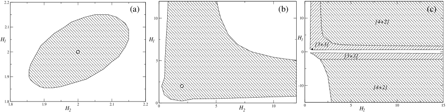
Figure 1: Typical stability areas for vacuum $K_{3}\to K_{1}$ regime on (a) panel; vacuum and $\Lambda$-term $K_{3}\to E_{3+2}$ regime on (b) panel; vacuum and $\Lambda$-term $K_{3}\to E_{3+3}$ (and possibly higher number of extra dimensions as well) regime on (c) panel (see the text for more details).

To summarize the results for the vacuum case, only $K_{3}\to E_{3+2}$ – the transition from GB Kasner to anisotropic exponential solution – is stable. All other regimes – transitions to isotropic exponential solution and to GR Kasner – have much smaller stability areas and could be called “metastable”. Formally, the basin of attraction of $K_{1}$ and isotropic expansion is nonzero and they are stable within it, but on the other hand its area is much smaller then that of $E_{3+2}$; so that comparing with the two we decided to call $K_{3}\to E_{3+2}$ as “stable” while $K_{3}\to K_{1}$ and $K_{3}\to E_{iso}$ as “metastable”.

Now let us consider $\Lambda$-term case. According to my16b , in the presence of $\Lambda$-term the variety of the regimes is a bit different from the vacuum case. Again, there are two branches ($h_{1}$ and $h_{2}$) and now in addition to variation in $\alpha$ there is variation in $\Lambda$ and in their product $\alpha\Lambda$.

The first case is $\alpha>0$, $\Lambda>0$. There on $h_{1}$ branch we have $K_{3}\to E_{3+2}$ if $\alpha\Lambda\leqslant 1/2$ and $K_{3}\to nS$ if $\alpha\Lambda>1/2$. Another ($h_{2}$) branch has $K_{3}\to E_{iso}$ regardless of $\alpha\Lambda$. All these three branches are stable – breaking the symmetry of both subspaces keeps the regimes as they are within wide vicinity of the exact solution, like in Fig. 1(b). Stable solution $K_{3}\to E_{iso}$ as a future attractor for broken symmetry in both subspaces is illustrated in Fig. 2(b). The next case to consider is $\alpha>0$, $\Lambda<0$; there $h_{1}$ branch has $K_{3}\to E_{3+2}$ while $h_{2}$ has $K_{3}\to nS$ and the former of them is proved to be stable (the latter is not viable so its stability is of little importance). Now let us turn to $\alpha<0$ cases and the first one is with $\Lambda>0$. There at $\alpha\Lambda\geqslant-5/6$ both branches have $K_{3}\to E_{iso}$ regime and both of them are metastable – only the initial conditions which are very close to the exact solution lead to $E_{iso}$, those beyond lead to $nS$. On contrary, at $\alpha\Lambda<-5/6$ on $h_{1}$ branch we have $K_{3}\to E_{3+2}$ while on $h_{2}$ branch $K_{3}\to nS$ and again $E_{3+2}$ is stable. Finally, $\alpha<0$, $\Lambda<0$ has $K_{3}\to E_{iso}$ on $h_{1}$ and $K_{3}\to nS$ on $h_{2}$ and in this case $E_{iso}$ is stable.

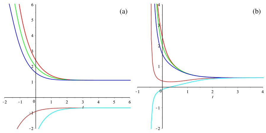
Figure 2: Typical evolution curve for stable anisotropic (a) and isotropic (b) exponential solutions with broken symmetry in both subspaces in the $D=2$ case (see the text for more details).

In addition to the described above $D=2$ case, we also considered $D=3$. The methodology is the same and the results for vacuum $K_{3}\to K_{1}$ are also the same. But the results for both vacuum and $\Lambda$-term $K_{3}\to E_{3+3}$ transition are different and presented in Fig. 1(c), where the initial conditions leading to $E_{3+3}$ are shaded with $[3+3]$ note on them. One can see that the stability area is unbounded, as it was in $D=2$ case, but there are differences as well. First, the upper part seems shrinked in comparison with $D=2$ - so that starting from a vicinity of the exact solution, it is less probable to end up on $E_{3+3}$. Instead, we have $K_{3}\to E_{4+2}$ – the exponential solution with four expanding and two contracting dimensions, which is, obviously, non-viable. In Fig. 3 we presented $K_{3}\to E_{3+3}$ in (a) panel and $K_{3}\to E_{4+2}$ in (b) panel with the latter originates from some vast vicinity of the former. We also have some initial conditions starting from the negative values to lead to the exponential solution (which could “compensate” the loss in the upper part) – something we have never seen in $D=2$ – but this is the effect of the number of dimensions – in $D=2$, due to the lesser number of dimensions, the constraint is more tight while in $D\geqslant 3$ it is more relaxed. The presence of the $E_{4+2}$ is also the effect of the higher number of extra dimensions – indeed, as we demonstrated in CPT1 , in five spatial dimensions there is only one stable anisotropic exponential solution – $E_{3+2}$ (see my15 ; iv16 for stability issues), while in six and higher there are more CPT3 and there is a chance to end up on another exponential solution. As the number of exact solutions grow up with the number of dimensions, in higher dimensions it is probable to end up on another exponential solution, rather then $E_{3+D}$.

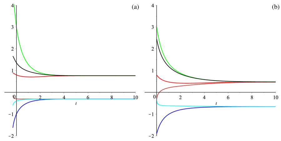
Figure 3: Typical evolution curve for stable anisotropic $[3+3]$ (a) and $[4+2]$ (b) exponential solutions with broken symmetry in both subspaces in the $D=3$ case (see the text for more details).

The black circle in Fig. 1(c) corresponds to the exact $E_{3+3}$ solution and one can see that the initial conditions are aligned along $H_{i}^{(0)}\sim H_{j}^{(0)}$. The same could be seen from $D=2$ case as well (see Fig. 1(b)). The reason for it is quite clear – indeed, with appropriate $H_{i}^{(0)}=H_{j}^{(0)}$ the exact $E_{3+D}$ solution is achieved explicitly, so that it is natural for the initial conditions to tend to this relation.

To conclude, we see that all $K_{3}\to E_{3+D}$ regimes in $\Lambda$-term case are stable with respect to breaking the symmetry of both subspaces. On the other hand, another nonsingular regime, $K_{3}\to E_{iso}$ is stable only for ($\alpha>0$, $\Lambda>0$) and ($\alpha<0$, $\Lambda<0$). Finally, $K_{3}\to K_{1}$ in vacuum is also stable, but its basin of attraction is quite small and any substantial deviation from the exact solution destroys it.

V Two-step scheme for general spatially curved case

The results of two previous sections allow us to construct a scenario of compactification which satisfy two important requirements:

• the evolution starts from a rather general anisotropic initial conditions,

• the evolution ends in a state with three isotropic big expanding dimensions and stabilized isotropic extra dimensions.

The first part of the scenario in question uses the results of Sec. IV. We have seen there that while starting from a state in the dashed zone of Fig. 1(b),(c) the flat anisotropic Universe tends to the exponential solution with three equal expanding dimensions. The initial conditions for such a behavior are not so restricted. From the Fig. 1(b) we can see that initial state should already have three expanding and two shrinking dimensions, however, since all Gauss-Bonnet Kasner solutions (as well as usual GR Kasner solutions) should have et least one shrinking dimension, this requirement does not constraint possible initial state very seriously – in any cases we should expect that contracting dimensions are present in the initial conditions. Within this situation the dashed zone occupy rather big part of initial condition space of Fig. 1(b), and any solution from this zone ends up in exponential solution of desired type.

In higher dimensions the situation is from one side worsening – as it is seen from Fig. 1(c), in $D\geqslant 3$ there are more then one stable anisotropic exponential solution, so that starting from the vicinity of exact $E_{3+3}$ solution we could end up in $E_{4+2}$ solution, which does not has realistic compactification. However, from the other side, initial conditions with 2 expanding and 4 contracting dimensions can end up in 3+3 exponential solution.

Suppose also, that a negative spatial curvature is small enough at the beginning and starts to be important only after this transition to exponential solution (which is established in the present paper only for a flat Universe) already occurred. This condition allows us to glue the second part of the scenario which requires negative spatial curvature of the inner space. We have see in Sec. III that exponential solution turn to the solution with stabilized extra dimensions in this case. As a result of these two stages a Universe starting from initially anisotropic both outer expanding three dimensional space and contracting inner space evolves naturally to the final stage with isotropic three big dimensions and isotropic and stabilized inner dimensions. The only additional condition for this scenario to realize (in addition to starting from the appropriate zone in the initial conditions space) is that spatial curvature should become dynamically important only after the transition to exponential solution occurs. As we mentioned in Sec. III, this part (and so the entire scheme as well) works only for $D\geqslant 3$.

VI Discussions and conclusions

Prior to this paper, we completed study of the most simple (but the most important as well) cases. The spatial part of these cases is the product of three- and extra-dimensional subspaces which are spatially flat and isotropic my16a ; my16b ; my17a . So that the obvious next step is consideration of these subspaces being non-flat and anisotropic, and that is what we have done in current paper. Non-flatness is addressed by assuming that both subspaces have constant curvature while anisotropy – by breaking the symmetry between the spatial directions. The results of the curvature study suggest that the only viable regimes are those from the flat case with $\gamma_{\left(\mathbf{D}\right)}=0$ requirement. Additionally, in the $\Lambda$-term case there is “geometric frustration” regime, described in CGP1 ; CGP2 and further investigated in CGPT with $\gamma_{\left(\mathbf{D}\right)}<0$ requirement.

Our study reveals that there is a difference between the cases with $\gamma_{\left(\mathbf{D}\right)}=0$ and $\gamma_{\left(\mathbf{D}\right)}<0$: the former of them have only exponential solutions and the isotropic and anisotropic solutions coexist; the latter have the regime with stabilization of the extra dimensions (instead of “pure” anisotropic exponential regime) and isotropic exponential regimes cannot coexist with regimes of stabilization – this difference was not noted before. The curvature effects also differ in different $D$ – in $D=2$ there is no stabilization of extra dimensions while in $D\geqslant 3$ there is.

In $D=3$ and $\gamma_{\left(\mathbf{D}\right)}<0$ there is also an interesting regime in the vacuum case – the regime with stabilization of one and power-law expansion of another three-dimensional subspaces; viability of this regime for some compactification scenario needs further investigations.

The results of anisotropy study reveal that the $K_{3}\to E_{3+D}$ regime is always stable with respect to breaking the isotropy in both subspaces, meaning that within some vicinity of exact $K_{3}\to E_{3+D}$ transition, all initial conditions still lead to this regime (see Fig. 2(a)). Though, the area of the basin of attraction for this regime depends on the number of extra dimensions $D$ – in $D=2$ it is quite vast (see Fig. 1(b)) and there are no other anisotropic exponential solutions, in $D=3$ (and higher number of extra dimensions) it seems smaller and there are initial conditions in the vicinity of $E_{3+D}$ which leads to other exponential solutions. In our particular example $D=3$, presented in Fig. 1(c), some of the initial conditions from the vicinity of $E_{3+3}$ end up in $E_{4+2}$ instead. We expect that in higher number of extra dimensions the situation for $E_{3+D}$ would be more complicated and requires a special analysis.

Another viable regime, $K_{3}\to K_{1}$ from the vacuum case, as well as other non-viable regimes, are “metastable” – formally they are stable, but their basin of attraction is much smaller compared to that of $E_{3+D}$ (see Fig. 1(a)).

Our study clearly demonstrates that the dynamics of the non-flat cosmologies could be different from flat cases and even some new regimes could emerge. In this paper we covered only the simplest case with constant-curvature subspaces leaving the most complicated cases aside – we are going to investigate some of them deeper in the papers to follow.

Now with both effects – the spatial curvature and anisotropy within both subspaces – being described, let us combine them. In the totally anisotropic case, as we demonstrated, wide area of the initial conditions leads to anisotropic exponential solution (for the values of couplings and parameters when isotropic exponential solutions do not exist). So that if we start from the some vicinity of the exact exponential solution, and if the initial scale factors are large enough for the curvature effects to be small, we shall reach the anisotropic exponential solution with expanding three and contracting extra dimensions. After that the curvature effects in the expanding subspace are nullified while in the contracting dimensions they are not. If it is vacuum case, as we shown earlier, as long as $\gamma_{\left(\mathbf{D}\right)}\neq 0$ we encountered nonstandard singularity, so that the vacuum case is pathological in this scenario. In the $\Lambda$-term case, as we reported earlier, for $\gamma_{\left(\mathbf{D}\right)}=0$ we recover the same exponential regime, for $\gamma_{\left(\mathbf{D}\right)}>0$ the behavior is singular and only for $\gamma_{\left(\mathbf{D}\right)}<0$ we obtain $E_{C,0}$ – “geometric frustration” scenario CGP1 ; CGP2 with stabilization of the extra dimensions.

So that we can see that the proposed two-steps scheme works only for the $\Lambda$-term case and only if $\gamma_{\left(\mathbf{D}\right)}<0$ – in all other cases it either provides trivial regimes, or leads to singular behavior. Also, there is a minor problem with the number of extra dimensions – as we noted, the first stage of this scheme – reaching the exponential asymptote from initial anisotropy – best achieved in $D=2$ and the probability of reaching $E_{3+D}$ could decrease with growth of $D$. On the other hand, the second stage – when the negative curvature changes the contracting exponential solution for the extra dimensions into stabilization – is not presented in $D=2$ and only manifest itself in $D\geqslant 3$. So that the described two-stages scheme works only in $D\geqslant 3$ and in this case the initial conditions for the first stage are already not so wide, though a fine-tuning of initial conditions is not needed.

This finalize our paper. The presented analysis suggests that more in-depth investigation of both curvature and anisotropy effects are required – we have investigated and described the most simple but still very important cases – constant-curvature and flat anisotropic (Bianchi-I-type) geometries; in the papers to follow we are going to consider more complicated topologies.

- (1) G. Nordström, Phys. Z. 15, 504 (1914).
- (2) A. Einstein, Ann. Phys. (Berlin) 354, 769 (1916).
- (3) T. Kaluza, Sit. Preuss. Akad. Wiss. K1, 966 (1921).
- (4) O. Klein, Z. Phys. 37, 895 (1926).
- (5) O. Klein, Nature (London) 118, 516 (1926).
- (6) J. Scherk and J.H. Schwarz, Nucl. Phys. B81, 118 (1974).
- (7) P. Candelas, G.T. Horowitz, A. Strominger and E. Witten, Nucl. Phys. B258, 46 (1985).
- (8) B. Zwiebach, Phys. Lett. 156B, 315 (1985).
- (9) C. Lanczos, Z. Phys. 73, 147 (1932).
- (10) C. Lanczos, Ann. Math. 39, 842 (1938).
- (11) B. Zumino, Phys. Rep. 137, 109 (1986).
- (12) D. Lovelock, J. Math. Phys. (N.Y.) 12, 498 (1971).
- (13) F. Mller-Hoissen, Phys. Lett. 163B, 106 (1985).
- (14) N. Deruelle and L. Fariña-Busto, Phys. Rev. D 41, 3696 (1990).
- (15) F. Mller-Hoissen, Class. Quant. Grav. 3, 665 (1986).
- (16) J. Demaret, H. Caprasse, A. Moussiaux, P. Tombal, and D. Papadopoulos, Phys. Rev. D 41, 1163 (1990).
- (17) G. A. Mena Marugán, Phys. Rev. D 46, 4340 (1992).
- (18) E. Elizalde, A.N. Makarenko, V.V. Obukhov, K.E. Osetrin, and A.E. Filippov, Phys. Lett. B644, 1 (2007).
- (19) K.I. Maeda and N. Ohta, Phys. Rev. D 71, 063520 (2005).
- (20) K.I. Maeda and N. Ohta, JHEP 1406, 095 (2014).
- (21) F. Canfora, A. Giacomini and S. A. Pavluchenko, Phys. Rev. D 88, 064044 (2013).
- (22) F. Canfora, A. Giacomini and S. A. Pavluchenko, Gen. Rel. Grav. 46, 1805 (2014).
- (23) F. Canfora, A. Giacomini, S. A. Pavluchenko and A. Toporensky, arXiv:1605.00041.
- (24) D.G. Boulware and S. Deser, Phys. Rev. Lett. 55, 2656 (1985).
- (25) J.T. Wheeler, Nucl. Phys. B268, 737 (1986).
- (26) R.G. Cai, Phys. Rev. D 65, 084014 (2002).
- (27) T. Torii and H. Maeda, Phys. Rev. D 71, 124002 (2005).
- (28) T. Torii and H. Maeda, Phys. Rev. D 72, 064007 (2005).
- (29) D.L. Wilshire. Phys. Lett. B169, 36 (1986).
- (30) R.G. Cai, Phys. Lett. 582, 237 (2004).
- (31) J. Grain, A. Barrau, and P. Kanti, Phys. Rev. D 72, 104016 (2005).
- (32) R. Cai and N. Ohta, Phys. Rev. D 74, 064001 (2006).
- (33) X.O. Camanho and J.D. Edelstein, Class. Quant. Grav. 30, 035009 (2013).
- (34) H. Maeda, Phys. Rev. D 73, 104004 (2006).
- (35) M. Nozawa and H. Maeda, Class. Quant. Grav. 23, 1779 (2006).
- (36) H. Maeda, Class. Quant. Grav. 23, 2155 (2006).
- (37) M. Dehghani and N. Farhangkhah, Phys. Rev. D 78, 064015 (2008).
- (38) N. Deruelle, Nucl. Phys. B327, 253 (1989).
- (39) S.A. Pavluchenko, Phys. Rev. D 80, 107501 (2009).
- (40) S.A. Pavluchenko and A.V. Toporensky, Mod. Phys. Lett. A24, 513 (2009).
- (41) S.A. Pavluchenko, Phys. Rev. D 82, 104021 (2010).
- (42) V. Ivashchuk, Int. J. Geom. Meth. Mod. Phys. 07, 797 (2010) arXiv: 0910.3426.
- (43) I.V. Kirnos, A.N. Makarenko, S.A. Pavluchenko, and A.V. Toporensky, Gen. Rel. Grav. 42, 2633 (2010).
- (44) S.A. Pavluchenko and A.V. Toporensky, Gravitation and Cosmology 20, 127 (2014); arXiv: 1212.1386.
- (45) H. Ishihara, Phys. Lett. B179, 217 (1986).
- (46) I.V. Kirnos, S.A. Pavluchenko, and A.V. Toporensky, Gravitation and Cosmology 16, 274 (2010) arXiv: 1002.4488.
- (47) D. Chirkov, S. Pavluchenko, A. Toporensky, Mod. Phys. Lett. A29, 1450093 (2014); arXiv: 1401.2962.
- (48) D. Chirkov, S. Pavluchenko, A. Toporensky, Gen. Rel. Grav. 46, 1799 (2014); arXiv: 1403.4625.
- (49) D. Chirkov, S. Pavluchenko, A. Toporensky, Gen. Rel. Grav. 47, 137 (2015); arXiv:1501.04360.
- (50) S.A. Pavluchenko, Phys. Rev. D 92, 104017 (2015).
- (51) V. D. Ivashchuk, Eur. Phys. J. C 76, 431 (2016).
- (52) S.A. Pavluchenko, Phys. Rev. D 94, 024046 (2016).
- (53) S.A. Pavluchenko, Phys. Rev. D 94, 084019 (2016).
- (54) S.A. Pavluchenko, Eur. Phys. J. C 77, 503 (2017).
- (55) M. Brigante, H. Liu, R. C. Myers, S. Shenker and S. Yaida, Phys. Rev. D 77, 126006 (2008).
- (56) M. Brigante, H. Liu, R. C. Myers, S. Shenker and S. Yaida, Phys. Rev. Lett. 100, 191601 (2008).
- (57) A. Buchel and R. C. Myers, JHEP 0908, 016 (2008).
- (58) D. M. Hofman, Nucl. Phys. B823, 174 (2009).
- (59) J. de Boer, M. Kulaxizi and A. Parnachev, JHEP 1003, 087 (2010).
- (60) X. O. Camanho, J. D. Edelstein, JHEP 1004, 007 (2010).
- (61) A. Buchel, J. Escobedo, R. C. Myers, M. F. Paulos, A. Sinha and M. Smolkin, JHEP 1003, 111 (2010).
- (62) X.-H. Ge and S.-J. Sin, JHEP 0905, 051 (2009).
- (63) R.G. Cai and Q. Guo, Phys. Rev. D 69, 104025 (2004).
- (64) S.A. Pavluchenko, Phys. Rev. D 67, 103518 (2003).
- (65) S.A. Pavluchenko, Phys. Rev. D 69, 021301 (2004).
- (66) J.A. Wolf, Spaces of constant curvature, 4th edition (Publish or Perish, Wilmington, Delaware USA, 1984), p. 69.
- (67) F.J. Tipler, Phys. Lett. A64, 8 (1977).
- (68) T. Kitaura and J.T. Wheeler, Nucl. Phys. B355, 250 (1991).
- (69) T. Kitaura and J.T. Wheeler, Phys. Rev. D 48, 667 (1993).