Multi-scale Forest Species Recognition Systems for Reduced Cost

Abstract

This work focuses on cost reduction methods for forest species recognition systems. Current state-of-the-art shows that the accuracy of these systems have increased considerably in the past years, but the cost in time to perform the recognition of input samples has also increased proportionally. For this reason, in this work we focus on investigating methods for cost reduction locally (at either feature extraction or classification level individually) and globally (at both levels combined), and evaluate two main aspects: 1) the impact in cost reduction, given the proposed measures for it; and 2) the impact in recognition accuracy. The experimental evaluation conducted on two forest species datasets demonstrated that, with global cost reduction, the cost of the system can be reduced to less than 1/20 and recognition rates that are better than those of the original system can be achieved.

1 Introduction

Automatic forest species recognition has been drawing the attention of the research community, given its both commercial and environment-preserving value. For example, by better monitoring wood timber trading, one may reduce commercialization of samples from species that are forbidden to be traded, e.g. species near extinction. However, in most cases, the wood being traded has been cut into pieces of lumber, and identifying the forest species which those wood lumbers come from generally requires an expert. For this reason, an automatic system for forest species recognition consists of an alternative to reduce the costs of hiring and training human experts and, hopefully, a way to improve the speed and accuracy in performing this task.

In the image recognition community, we observe that forest species recognition has been generally treated as an image texture recognition problem [1, 2, 5, 9, 12, 13, 15, 19, 4]. In contrast with image object recognition, where most of the shape of the object must be visible so as for a class to be associated to it, texture recognition can be conducted only on a small portion of the whole. As a result, significant improvements in forest species recognition accuracy can be achieved with the use of multiple classifiers or multiple classifications. In [15], it is demonstrated that higher recognition rates can be achieved by dividing the images into sub-segments, and combining their individual classification results. Boost in the recognition rates can also be observed by making use of multiple feature sets [12], or even by combining both ideas as in the multiple feature vector framework proposed in [4].

Despite the improvement in recognition accuracy that multiple classifiers or multiple classifications can bring to the forest species recognition task, a major drawback is the considerable increase in the computational cost that is required to carry out the recognition of an input sample. When multiple feature sets are used, the cost increases linearly with the number of feature sets. When the images are divided into sub-segments, the cost can increase quadratically.

Given these standpoints, the main contribution of this paper lies in investigating and proposing methods to reduce the costs of this type of system using multiple classifications, with minimum impact on the recognition accuracy. To achieve this, we present investigations on cost reduction at different levels of a forest species recognition system. First, in Section 4, we introduce the Adaptive Multi-Level Framework (AMLF), which consists of an adaptive system for cost reduction at classification level. Next, in Section 5, we present an evaluation of cost reduction at feature extraction level, where the resolution of the images are reduced to different scale ratios. Then, Section 6 provides an analysis of cost reduction at global level, combining both feature extraction and classification cost reduction. It is worth mentioning that cost reduction for these evaluations are measured based on definition of cost presented in Section 3, where we focus on texture-based feature extraction methods and Support Vector Machine (SVM) classifiers. The results show that not only the cost can be very successfully reduced to about 1/20 of the original methods, but also better recognition rates can observed with the proposed methods.

2 State of the Art

The recognition of forest species images can be divided into two approaches: microscopic and macroscopic. In the former, the image acquisition protocol is more complex since it depends on several procedures such as boiling the wood, cut it with a microtone, and dehydrating the slides, before acquiring the images. The result, though, is an image full of the details that can be useful to discriminate similar classes. This complex acquisition protocol, on the other hand, does not make the microscopic approach suitable to be used in the field, where one needs less expensive and more robust hardware [16]. To overcome this problem, some authors have investigated the use of macroscopic images to classify forest species. Figure 1 and Figure 2 compares the microscopic and macroscopic samples of the the same forest species (Pinacae Pinus Taeda). As one may observe the macroscopic image has a significative loss of information when compared to the microscopic one.

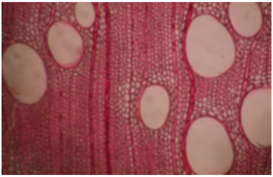
Figure 1: Samples of a microscopic image of Pinacae Pinus Taeda [16]

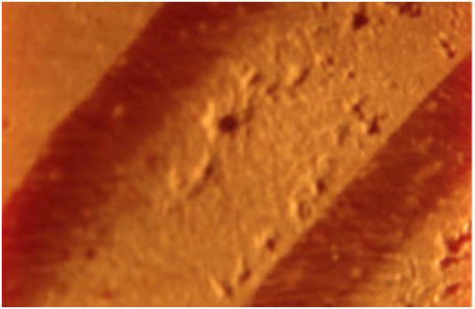
Figure 2: Samples of a macroscopic image of Pinacae Pinus Taeda [16]

Reviewing the literature of forest species recognition using macroscopic images, we may notice that the early works used mainly neural netwoks (multi-layer perceptron in most cases) and Gray-Level Co-ocurrence Matrices (GLCM) as features [17, 18, 19, 8]. More recently, other representations such as Gabor filters [23], Local Binary Patterns (LBP) [14], Local Phase Quantization (LPQ) [16] and more robust classification schemes, such as ensembles of classifiers, were adopted, hence, raising the recognition rates. Systems based on representation learning using Convolutional Neural Networks (CNN) also have been exploited producing interesting results [6]. Table 1 summarizes the works on forest species recognition using macroscopic images.

Table 1: Summary of the works on forest species recognition.

Authors.	Features	Images/	Rec. Rate
		Classes	(%)
Tou et al. [17]	GLCM	360/5	72.0
Tou et al. [18]	GLCM, 1DGLCM	360/5	72.8
Tou et al. [19]	GLCM, Gabor, GLCM	600/6	85.0
Khalid et al. [8]	GLCM	1949/20	95.0
Yusof et al. [23]	Gabor, GLCM	3000/30	90.3
Nasirzadeh et al. [14]	LBPu2, LBPHF	3700/37	96.6
Paula Filho et al. [15]	Color, GLCM	1270/22	80.8
Hafemann et al. [6]	CNN	2942/41	95.7
Paula Filho et al. [16]	Color, CLBP, Gabor, LPQ	2942/41	97.7

Research on microscopic imagens is more recent and became more popular with the release of a public database composed of 2240 images of 112 different species (see Section 2.1), which made benchmarking and evaluation easier. Similarly to the literature on macroscopic images, most of the works on forest species using microscopic images use textural representation such as LBP [12], LPQ [12] and their variants [7, 11]. CNN also has been proved to be an interesting alternative for microscopic images [6]. Table 2 summarizes the works on forest species recognition using microscopic images.

Table 2: Summary of the results published in the literature using the microscopic images of forest species

Authors.	Features	Images/	Rec. Rate
		Classes	(%)
Yadav et al. [21]	Gabor+GLCM	500/25	88.0-92.0
Yusof et al. [22]	Basic Gray Level Aura Matrix	5200/52	89.0-93.0
Martins et al. [12]	LBP	2240/112	80.7
Martins et al. [12]	LPQ+LBP	2240/112	86.5
Cavalin et al. [4]	LPQ+GLCM	2240/112	93.2
Kapp et al. [7]	LPQ+LPQ-Blackman+LPQ-Gauss	2240/112	95.68
Hafemann et al. [6]	Convolutional Neural Network	2240/112	97.3
Martings et al. [11]	LBP+LPQ	2240/112	93.0
Yadav et al. [20]	Multiresolution LBP	1500/75	97.4

2.1 Datasets

In this section we describe the two Forest Species databases used in this work, namely microscopic database and macroscopic database, respectively.

The microscopic database, which is described in detail in [13], contains 112 different forest species catalogued by the Laboratory of Wood Anatomy at the Federal University of Paraná in Curitiba (UFPR), Brazil. These images were acquired with an Olympus Cx40 microscope equipped with a 100x zoom, after the wood went through some chemical/physical steps such as boiling, veneer coloring, and dehydration. In total, the dataset contains 2,240 microscopic images, with a resolution of 1,024 by 768 pixels, equally distributed into set of 112 classes. It is worth mentioning that 37 of the classes correspond to Softwood species, while 75 consist of Hardwood.

The macroscopic database was also catalogued by the Laboratory of Wood Anatomy at UFPR, and it is composed of 2,942 samples of 41 distinct species. In this case, though, the images were captured with a Sony DSC T20 digital camera, resulting in image with a resolution of 3,264 by 2,448. The number of samples per class ranges from 37 to 99, with an average of 71.75. Greater detail about this dataset can be found in [16].

3 General Cost Definition

The meaning of what we refer to as cost basically represents the time required for recognizing an image, or a set of test images (in considering that the different methods involved in the cost analysis are evaluated on the same set). Although one can directly measure the running time of a given application to process such a set, and simply compare the differences among implementations of different systems, some factors such as operating system workload can affect this method even if the operating system, programming language and hardware used to implement and run the systems are exactly the same.

In consequence, we define cost in a more general form, which can be applied to any distinct implementation, based on counting the total number of basic operations that are necessary to recognize the set of samples. The basic operation can be defined differently depending on which part of the system we need to evaluate, or using an operation that is common for all parts.

Let $Ne$ be the number of samples in the test set, in a general form, cost can be defined as:

$$Cost=\sum_{i=1}^{Ne}(Cost^{F}+Cost^{C}),$$ (1)

where $Cost^{F}$ corresponds to the cost of feature extraction, and $Cost^{C}$ to the cost of classification.

In the next sections we present in details ways to measure $Cost^{C}$ and $Cost^{F}$, respectively, and how reducing their values impacts recognition accuracy, either individually or combined.

4 Classification Cost Reduction

In this section, we present the proposed approach named Adaptive Multi-Level Framework (AMLF), the main goal of which is to perform forest species recognition with accuracy close to the Single-Level Multiple Feature Vector Framework (SLF), proposed in [4], but with reduced cost at classification level.

Basically, AMLF consists of layers of different versions of SLF, with varied costs, and the main idea is to rely on less costly but less accurate layers of SLF first, then move to more costly and consequently more accurate layers depending in the difficulty to recognize a given sample.

Before describing the aforementioned approaches, we first define a way to measure classification cost.

4.1 Classification Cost Definition

In this section we specify Equation 1 to compute cost at classification level, allowing further to compare the cost of AMLF with different versions of SLF. Thus, given that feature extraction cost reduction is out of the scope of this section, we first adapt that equation to consider only classification:

$$Cost^{\prime}=\sum_{i=1}^{Ne}Cost^{C}.$$ (2)

The previous equation is too general, so we need to define a way to compare the different approaches based on basic operations. Given that the main difference between the approaches that we consider in this paper is the number of classifications performed for a sample, the basic operation is herein defined as a classification step performed by a classifier, i.e. running a classification algorithm until a classification output comes out. Thus, let $f_{i}$ be a function that returns the number of classifications needed to recognize the $i$-th test sample, $Cost^{\prime}$ can be defined as:

$$Cost^{\prime}=\sum_{i=1}^{Ne}f_{i}.$$ (3)

Nonetheless, another cost factor must also be considered. Depending on the type of base classifier, a classification might be more costly than others, i.e. it might require more time to be conducted. For this reason, we extend the previous equation to:

$$Cost^{\prime}=\sum_{i=1}^{Ne}{(f_{i}\times\Gamma_{i})},$$ (4)

where $\Gamma_{i}$ represent the cost of the base classifier, which may be, for instance, the size (the number of hidden neurons) of a Multilayer Perceptron Neural Network or the number of support vectors for Support Vector Machines (SVMs) (similarly to the total number of feature values (TVF) measure [10]), to weigh the classification operation.

Next, we describe the framework presented in [4] and how Equation 4 can be adapted for this specific system.

4.2 Single-Level Multiple Feature Vector Framework (SLF)

The main idea of SLF lies in using information from multiple feature vectors to improve recognition performance, owing to the variability introduced by these multiple vectors. One way to do so is with the extraction of diverse feature vectors by both dividing the input image into sub-images (or patches, which is a term that we use interchangeably), and by combining different feature sets, as depicted in Figure 3.

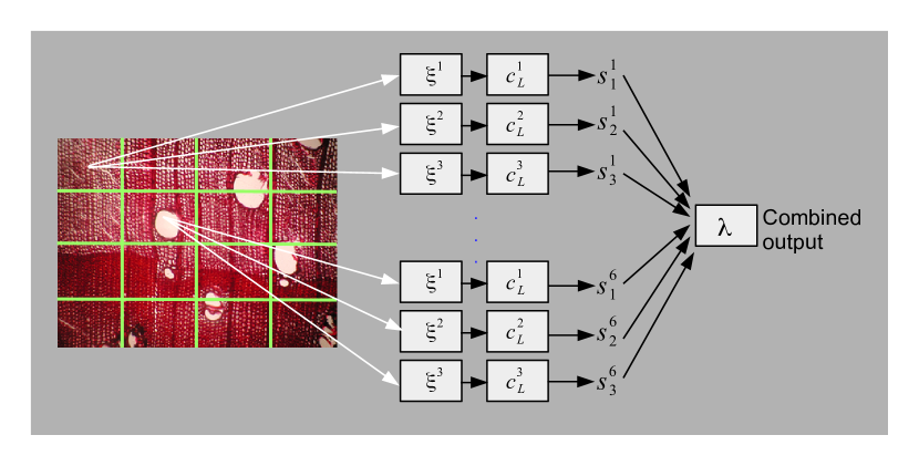
Figure 3: Overview of the SLF method. In this example, three feature sets are extracted from $im^{\prime}_{1}$ and $im^{\prime}_{6}$, resulting in output $s^{1}_{j}$ and $s^{6}_{j}$.

The main steps of SLF are listed in Algorithm 1. The inputs for this algorithm are: the original image, denoted $im$; the parameter $L$, to define the number of patches in which $im$ will be divided; the set of feature sets $\Xi=\{\xi^{1},\ldots,\xi^{M}\}$, where $\xi^{j}$ represents a distinct feature set with $m^{j}$ features, and $M=|\Xi|$ corresponds to the total number of feature sets; the set of classifiers $C_{L}=\{c_{L}^{1},\ldots,c_{L}^{M}\}$, corresponding to the set of classifiers trained for a given value of $L$ for each $\xi^{j}$; the number of classes of the problem denoted $K$; and a fusion function $\lambda$. From these inputs, the first steps consist in dividing the input image into $N$ sub-images. That is, in step 2, the number of patches $N$ is computed as a function of $L$, e.g. $N=f(L)$. Then, in step 3, $im$ is divided into $N$ non-overlapping sub-images with identical sizes, generating the set $I=\{im^{\prime}_{1},\ldots,im^{\prime}_{N}\}$. Next, the feature extraction is carried out. In steps 4 to 8, for each image $im^{\prime}_{i}$ in $I$ and each feature set $\xi^{j}$ in $\Xi$, the feature vector $v_{i}^{j}$ is extracted and saved in $V$. Afterwards, each feature vector $v_{i}^{j}$ in $V$ is classified by the corresponding classifier $c_{L}^{j}$, resulting in the scores $s_{i}^{j}(k)$ for every class $k$, where $1\leq k\leq K$. Finally, all the scores $s_{i}^{j}(k)$ are combined using the combination function $\lambda$ and the final recognition decision $\phi$ is made, i.e. the forest species (a class $k$) from which $im$ has been extracted is outputted.

Algorithm 1 The main steps of SLF.

1:  Input: $im$, the input image; $L$, the parameter to compute the number of patches to divide $im$; $\Xi=\{\xi^{1},\ldots,\xi^{M}\}$, the collection of feature sets, where $\xi^{j}$ corresponds to a distinct feature set; $C_{L}=\{c_{L}^{1},\ldots,c_{L}^{M}\}$, the set of classifiers trained for the given $L$, for each $\xi^{j}$; $K$, the number of classes of the problem; and $\lambda$, a fusion function to combine multiple classification results.

2:  $N=f(L)$

3:  Divide $im$ into $N$ non-overlapping sub-images with equal size, generating the set $I=\{im^{\prime}_{1},\ldots,im^{\prime}_{N}\}$

4:  for each image $im^{\prime}_{i}$ in $I$ do

5:     for each feature set $\xi^{j}$ in $\Xi$ do

6:        Extract feature vector $v_{i}^{j}$ from $im_{i}$ by considering $\xi^{j}$ as feature set, and save $v_{i}^{j}$ in $V$

7:     end for

8:  end for

9:  for each feature vector $v_{i}^{j}$ in $V$ do

10:     Recognize $v_{i}^{j}$ using classifier $c_{L}^{j}$, and save the scores $s_{i}^{j}(k)$ for each class $k$, where $1\leq k\leq K$.

11:  end for

12:  Combine all scores $s_{i}^{j}(k)$ using $\lambda$, and compute output probabilities $P_{L}$.

We can adapt Equation 4 in order to parametrize the cost function according to the value of $L$, which affects the number of classifications, and the cost of the base classifier trained for level $L$. Consider that $f(L)$ returns the number of classifier calls needed for recognizing a testing sample with SLF at level $L$, and $\Gamma(C_{L})$ is a function that returns the cost of the classifiers in $C_{L}$. The cost $Cost^{\prime}_{SFL}(L)$ for SLF with level set to $L$ can be calculated with Equation 5.

$$Cost^{\prime}_{SLF}(L)=Ne\times f(L)\times\Gamma(L)$$ (5)

As shown in [4] (and also demonstrated in Section 4.4), the value of $L$ can greatly affect both recognition performance and cost. While an increase of more than 10 percentage points can be observed in accuracy by changing $L$ from 1 to 3, the number of classifications increases from 1 to 16. The cost increase is quadratic in this case. Furthermore, the same cost is required for all test samples no matter the difficulty level to conduct the recognition of each image. These are the reasons that inspired us to propose the adaptive framework described in Section 4.3.

4.3 Adaptive Multi-Level Framework (AMLF)

AMLF consists of evaluating consecutive layers of SLF, starting with layers with smaller values for $L$. If the level of confidence of the recognition result of such level is not high enough, $L$ is incremented and layers with bigger values are evaluated until the maximum level $L_{max}$ is reached, as illustrated in Figure 4. The level of confidence is computed based on the margin of the top two classes and a set of pre-defined thresholds, i.e. one threshold for each level $L<L_{max}$.

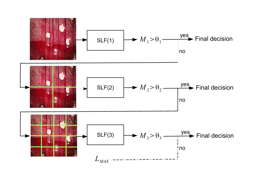
Figure 4: An illustration of AMLF.

This approach is better described in Algorithm 2. It consists of iterating the level value $l$ from 1 until $L_{max}$, the maximum value for $l$ (step 2). In step 3, Algorithm 1 (SLF) is called with the $L$ parameter set to $l$. The recognition probabilities computed in this iteration for image $im$ are saved in $P_{l}$. Next, in step 4, the margin $M_{l}$ is computed from $P_{l}$. If the value in $M_{l}$ is above the pre-defined threshold $\theta_{l}$ or the maximum level was reached, i.e. $l=L_{max}$, then the final recognition decision $\phi$ is computed and the algorithm stops (steps 5 to 8).

Algorithm 2 The AMLF approach.

1:  Input: $im$, the input image; $L_{max}$, the maximum number of layers; $\Xi=\{\xi^{1},\ldots,\xi^{M}\}$, the collection of feature sets, where $\xi^{j}$ corresponds to a distinct feature set; $C_{L}=\{c_{L}^{1},\ldots,c_{L}^{M}\}$, a set of classifiers trained for each $1\leq l\leq L_{max}$, for each $\xi^{j}$; $K$, the number of classes of the problem $\lambda$, a fusion function to combine multiple classification results; $\{\theta_{1},\ldots,\theta_{L_{max}-1}\}$, the rejection thresholds for each level.

2:  for $l$ from 1 to $L_{max}$ do

3:     Call SLF (Algorithm 1) with $L=l$ and save output probabilities in $P_{l}$

4:     Compute the margin $M_{l}$ using Equation 6

5:     if $M_{l}<\theta_{l}$ or $l==L_{max}$ then

6:        Compute the final recognition decision $\phi$

7:        Stop algorithm

8:     end if

9:  end for

Given that $P_{l}=\{p_{1},\ldots,p_{K}\}$ represents the set of probabilities computed for image $im$ at level $l$, the margin $M_{l}$ is computed according to Equation 6:

$$M_{l}=p_{i}-p_{j},$$ (6)

where $i=\operatorname*{arg\,max}_{k=1}^{K}p_{k}$ and $j=\operatorname*{arg\,max}_{j=1}^{K}p_{j}\ \forall j\neq i$.

The rejection thresholds are defined on the validation set using a two-step procedure. The first step consists of computing the minimum and maximum values of margin observed in the validation set for each level $l$, denoted $M^{\prime}_{l}$ and $M^{\prime\prime}_{l}$, respectively. This process relies on SLF only. In the second step, we evaluate the best combination of thresholds in ranges between $M^{\prime}_{l}$ and $M^{\prime\prime}_{l}$, using grid search. In this case, AMLF is used. After this process, the set of thresholds $\theta_{l}$ ($1\leq l<L_{max}$) that achieved the best recognition rates on the validation set are selected to be used during operation.

The cost for an implementation of AMLF can be computed by extending Equation 5. Let $Ne_{L}$ be the number of samples which AMLF exited at level $L$, and consider that the cost of recognizing theses samples correspond to the same cost of $Cost^{\prime}_{SLF}(L)$ in Equation 5 where $Ne=Ne_{L}$ plus the cost of all previous levels, i.e. $\sum{Cost^{\prime}_{SLF}(l)}$ for all $l<L$. The cost of AMLF can be computed as:

$$Cost^{\prime}_{AMLF}(L_{max})=\sum_{L=1}^{L_{max}}[Ne_{L}\times\sum_{l=1}^{L}(f(l)\times\Gamma(l))].$$ (7)

4.4 Experiments

In this section, we present the experiments to evaluate both the recognition rates achieved with AMLF, and the resulting cost associated to the system. These results are compared with the different versions of SLF that were used to compose AMLF. Details on how the methods were implemented can be found in [3].

4.4.1 Protocol

We consider both microscopic and macroscopic databases described in Section 2.1, and same experimental protocol defined in [4], allowing us to perform a direct comparison of the results.

The samples of each class have been partitioned in: 50% for training; 20% for validation; and 30% for test. Each subset has been randomly sampled with no overlapping between the sets. For avoiding the results to be biased to a given partitioning, this scheme is repeated 10 times. As a consequence, the results presented further represent the average recognition rate over 10 replications (each replication is related to different a partitioning).

As the base classifier, we make use of Support Vector Machines (SVMs) with Gaussian kernel. Parameters $C$ and $\gamma$ were optimized by means of a grid search with hold-out validation, using the training set to train SVM parameters and the validation set to evaluate the performance. After finding the best values for $C$ and $\gamma$, an SVM was trained with both the training and validation sets together. Note that normalization was performed by linearly scaling each attribute to the range [-1,+1].

The comparison between SLF and AMLF takes into account twelve different systems. For SLF there are 9 different systems varying in terms of the parameter $L$, which is set to 1, 2 and 3, and in terms of feature sets, given that we consider LBP and LPQ feature sets both individually and combined. For AMLF, we consider three different implementations. We set $L_{max}$ to 3 and varied the feature set, also making use of LBP and LPQ individually and combined.

The thresholds $\theta_{l}$, $1\leq l<L_{max}$ were set with a grid search of AMLF applying on the validation set, with classifiers trained only on the training set only to prevent from over fitting.

4.4.2 Results on the Microscopic dataset

In Figure 5 the average recognition rates of the twelve aforementioned systems are presented. The average recognition rates of 93.08% were the best ones in these experiments, achieved by SLF with LBP and LPQ feature sets and $L$ set to 3. With LBP only, the accuracy presented by SLF were of 88.50% with the same value for $L$, and with LPQ, 92.03%. The recognition rates of AMLF, with the same feature sets, were of 91.90%, 87,50%, 91.44%, for LBP and LPQ combined, LBP only, and LPQ only, respectively. Despite a small loss in average accuracy of AMLF compared with SLF with $L=3$, the standard deviation of the approaches show to that these systems resulted in similar recognition rates and, no significant loss of performance is observed with the use of AMLF.

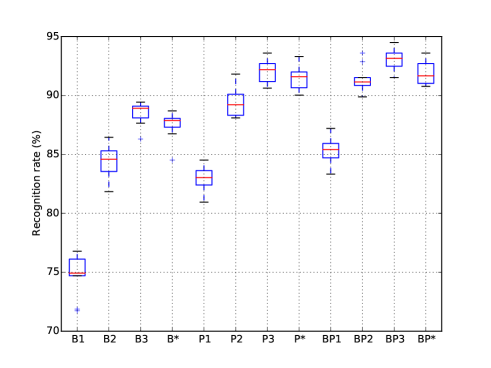
Figure 5: Recognition rates on the test set of the microscopic database, over 10 replications. B1, B2, B3: SLF with LBP and $L$ set to 1, 2 and 3, respectively; B*: AMLF with LBP feature set; the same notation is used for P1, P2, P3, P*, for the LPQ feature set, and BP1, BP2, BP3, BP* for both LBP and LPQ combined.

Besides that, the main advantage of the proposed AMLF becomes evident when the cost analysis is carried out, the results of which are depicted in Figure 6. In this case, SLF with LBP and LPQ combined and $L=3$ was on average about 10 times slower than AMLF with the same feature set. With LBP and LPQ individually, AMLF was generally almost 5 times faster than SLF. Note that the complexity can vary with the partitioning of the data set, especially in the experiment where the two feature sets were combined. Even with this variability, AMLF is at least twice as faster than SLF, but it can be also 16 times faster.

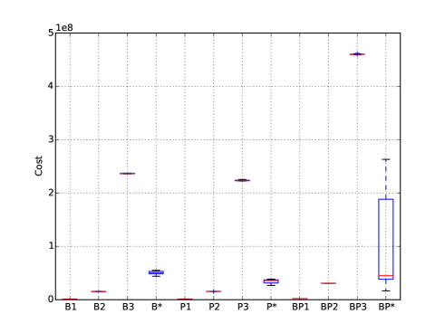
Figure 6: Overall time cost on the test set of the microscopic database, over 10 replications. B1, B2, B3: SLF with LBP and $L$ set to 1, 2 and 3, respectively; B*: AMLF with LBP feature set; the same notation is used for P1, P2, P3, P*, for the LPQ feature set, and BP1, BP2, BP3, BP* for both LBP and LPQ combined.

In order to complement this evaluation, in Figure 7 we present the average number of samples recognized in each level of AMLF (in which level the system stopped). We observe that when only one feature set is used, generally about for half of the samples it stops at level 1. Then, for about 33-39% of the samples it stops at level 2. And only about 13-16% of the samples were classified by level 3. With both LBP and LPQ feature sets combined, though, we observe that more samples are recognized at level 1, which is most given to the stronger classification scheme that is made by the combination of the feature sets.

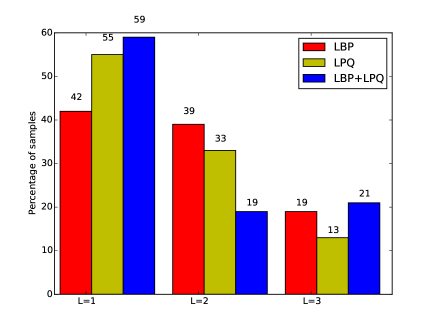
Figure 7: Average percentage of samples recognized at each level of AMLF with LBP, LPQ, and LBP and LPQ combined, respectively, on the microscopic dataset.

4.4.3 Results on the Macroscopic dataset

The recognition rates of the different systems, evaluated on the macroscopic dataset, are presented in Figure 8. Similarly to the results on the other dataset, SLF achieves slightly higher recognition rates. The best recognition rates, of about 92.81%, are achieved with SLF with LPQ features only and $L$ set to 3. With LBP features only, and LBP and LPQ combined, the accuracy was of 84.14% and 92.00%, respectively. The recognition rates of AMLF for LBP only, LPQ only, and LBP and LPQ combined, were of 83.97%, 92.63%, 91.86%. It is worth mentioning that there is a smaller difference between the results of SLF and AMLF with this dataset, making it more evident that the latter might present a performance that is similar to a costly version of the former.

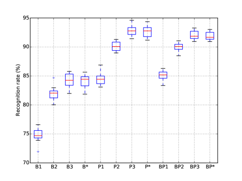
Figure 8: Recognition rates on the test set of the macroscopic database, over 10 replications. B1, B2, B3: SLF with LBP and $L$ set to 1, 2 and 3, respectively; B*: AMLF with LBP feature set; the same notation is used for P1, P2, P3, P*, for the LPQ feature set, and BP1, BP2, BP3, BP* for both LBP and LPQ combined.

The cost analysis for this dataset is presented in Figure 9. In this case, though, we observe that AMLF is not as faster as it can be in the microscopic dataset. With the best feature set, i.e. LPQ, AMLF is on average twice as faster than SLF with $L=3$. With LBP, it is on average 3 times faster. And with LBP and LPQ combined, AMLF is on average twice as faster, but depending on the partitioning of the dataset, it can be about 3 times faster or even have the same cost.

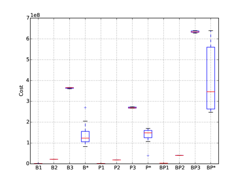
Figure 9: Overall time cost on the test set of the macroscopic database, over 10 replications. B1, B2, B3: SLF with LBP and $L$ set to 1, 2 and 3, respectively; B*: AMLF with LBP feature set; the same notation is used for P1, P2, P3, P*, for the LPQ feature set, and BP1, BP2, BP3, BP* for both LBP and LPQ combined.

The reason for the smaller difference in cost in this set can be easily visualized in Figure 10. In this case, we can observe that a similar amount of samples is recognized at level 1, i.e. from 33 to 46%. Nevertheless, much less samples are recognized at level 1, i.e. from 0 to 31%, and more samples at level 2, i.e. from 37 to 63%. With more samples being recognized at level 2, the more costly level, the cost of AMLF tends to get closer to the cost of SLF with $L=3$.

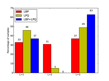
Figure 10: Average percentage of samples recognized at each level of AMLF with LBP, LPQ, and LBP and LPQ combined, respectively, on the macroscopic dataset.

5 Feature Extraction Cost Reduction

In this section, the focus is shifted to cost reduction at feature extraction level. The main idea to reduce this cost is pretty straight-forward, i.e. the image resolution can be reduced at a given scale $S$, where $0\leq S\leq 1$, and the feature extraction cost is reduced in the same proportion.

To make this idea clearer, in Section 5.1, we discuss in greater detail how resolution reduction affects the cost of feature extraction. Next, in Section 5.2, we present the experiments that have been conducted to evaluate the impact on the accuracy of SLF.

5.1 Feature Extraction Cost Definition

As we mentioned, feature extraction cost reduction can be directly measured by means of the scale factor $S$ acting in the resolution of the image. In other words, the feature extraction phase can be simplified as extracting features for all $P$ pixels in the image, and the larger the value of $P$, the more costly is this phase. Thus, the cost of feature extraction can be defined as:

$$Cost^{F}=P.$$ (8)

And given that in this particular section we do not consider the cost of classification, the overall cost $Cost^{\prime\prime}$ can be defined as:

$$Cost^{\prime\prime}=\sum_{i=1}^{Ne}Cost^{F}.$$ (9)

Nonetheless, if the resolution of the original image, containing $P$ pixels, is reduced by a scale factor $S$, where $0\leq S\leq 1$, then $Cost^{F}$ can be defined as a function of $S$:

$$Cost^{F}(S)=S\times P.$$ (10)

Note that $S$ consists only of a multiplication factor directly affecting $Cost^{F}$, defined in Equation 8. For this reason, $Cost^{F}(S)$ could be simply simplified to:

$$Cost^{F}(S)=S\times Cost^{F}.$$ (11)

And the overall cost can be simply defined as:

$$Cost^{\prime\prime}(S)=S\times Cost^{\prime\prime},$$ (12)

considering $Cost^{\prime\prime}$ defined in Equation 9.

5.2 Experiments

In this section we present the experiments to validate the impact of feature extraction cost reduction in the accuracy of different implementations of SLF, with $L$ ranging from 1 to 3, and with LBP, LPQ, and LBP and LPQ combined. The protocol used herein is the same as the one defined in Section 4.4.1.

In Figure 11 we provide the results on the microscopic dataset. We can observe that the feature extraction cost can be significantly reduced while maintaining or even surpassing the original recognition rates. Considering both LBP and LPQ combined, with $L=3$, the cost can be reduced to 40% ($S=0.4$) and better recognition rates are achieved, i.e. 93.97% compared with the 93.08% for $S=1.0$. For smaller values of $L$, the cost can be reduced to even smaller levels with no loss of performance. With $L$ set to 1, $S=0.2$ is about 2.67 percentage points better than $S=1.0$. And with $L$ set to 2, $S=0.3$ is about 0.7 percentage points better than $S=1.0$. A similar scenario can be observed with LBP, where the best recognition rates are achieved with $L$ set to 3 and $S=0.5$, reaching recognition rates of about 90.09%, compared with the 88.49% achieved with $S=1.0$. With LPQ, however, gains are only observed with $L$ set to either 1 or 2. With $L$ set to 3, $S$ can only be set to about 0.7 to keep the accuracy loss at minimum level.

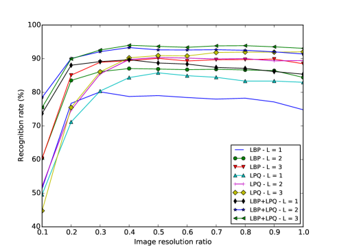
Figure 11: Average recognition rates with resolution scale $S$ from 0.1 to 1.0, in the microscopic dataset.

The corresponding evaluations on the macroscopic dataset are presented in Figure 12. In this case, reducing the cost of feature extraction generally results also on a positive impact on the recognition rates. Considering the combination of the both feature sets, the best recognition rates are achieved with $L=2$ and $S=0.1$, with recognition rates of about 96.58%. Compared with the best results with the original image, i.e. $L=3$ and $S=1.0$, this represents a gain of about 4.58 percentage points. In this case, for each configuration of $L$, $S=0.1$ always results in the best recognition rates, being the impact more significant on smaller values of $L$. With the feature sets used individually we observe a similar behavior. Considering LBP with $L=3$, $S=0.1$ represents a gain of 9.93 percentage points compared with $S=1.0$. And considering LPQ with $L=3$, $S=0.2$ results in a gain of 3.12 percentage points compared with $S=1.0$.

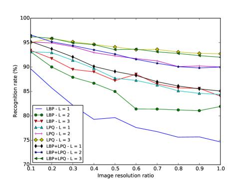
Figure 12: Average recognition rates with resolution scale $S$ from 0.1 to 1.0, in the macroscopic dataset.

6 Global Cost Reduction

After the presentation of methods that can be used successfully to reduce costs at either classification or feature extraction levels, in this section we evaluate how cost can be reduced for both levels at the same time, i.e. globally. That means, basically, the application of AMLF on images reduced by the scale factor $S$, and the evaluation of the impact on the recognition rates and on the cost.

To achieve this goal, we first describe a way to compute global cost, followed by the experimental evaluation.

6.1 Global Cost Definition

The fundamental issue related to computing cost at global level is the balance between the terms that represent the cost for feature extraction, i.e. $Cost^{F}$, and the cost for classification, i.e. $Cost^{C}$, in the $Cost$ defined in Equation 1. One solution that we propose is to take into account the dimension of the vectors involved in each phase, and the number of times a basic operation is applied on them. In this case, the basic operation is a multiplication involved in the dot product of two vectors. Let us first explain how this idea can be employed to compute $Cost^{F}$ and $Cost^{C}$, respectively, and then to compute the global costs for both SLF and AMLF.

By extending the ideas presented in Section 5.1, and considering that the feature extraction for all $P$ pixels involves applying a filter on the neighbourhood window of size $W$, the cost of feature extraction presented in Equation 8 can be extended in the following way:

$$Cost^{F}(S)=S\times(P\times W).$$ (13)

Similarly, for classification, we can add the $D$ term to represent the dimension of the vector inputed to the classifier, and define $Cost^{C}$ as:

$$Cost^{C}=\Gamma\times D,$$ (14)

where $\Gamma$ represents the cost of the base classifier, for instance the number of support vector in an SVM classifier.

Considering that the classification can take into account multiple classifiers, and the number of classifiers and the cost of the base classifier can be a function of $L$, we can extend Equation 14 to:

$$Cost^{C}(L)=f(L)\times(\Gamma(L)\times D).$$ (15)

As a result, the global cost for SLF, considering the scale factor $S$ and number of classifiers as a function of $L$, can be defined as:

$$Cost_{SLF}(L,S)=Ne\times(Cost^{F}(S)+Cost^{C}(L))$$ (16)

Similarly, considering also the scale factor $S$ and the maximum level as $L_{max}$, the global cost for AMLF can be defined as:

$$Cost_{AMLF}(S,L_{max})=\sum_{L=1}^{L_{max}}[Ne_{L}\times\sum_{l=1}^{L}[Cost^{F}(S)+Cost^{C}(L)]].$$ (17)

6.2 Experiments

In this section, we describe the experiments conducted to evaluate global cost reduction, using the same experimental described in Section 4.4.1. Basically, we compare the results of AMLF and SLF with $S=1.0$, with the best value of $S$ found in the results presented in Section 5.2, i.e. $S=0.4$ for microscopic and $S=0.1$ for macroscopic.

For the microscopic database, we present the recognition rates in Figure 13 and the costs in Figure 14. In terms of the recognition rates achieved by AMLF, we observe an increase from 91.90% to 93.17%. Furthermore, the gap between AMLF and SLF with $L=3$ decreases from 2.18 to 0.8 percentage points. In terms of cost, two aspects are worth mentioning. The first is that the average global cost of AMLF is reduced to about 1/3 of the cost of the original system, i.e. $S=1.0$. Moreover, it is also interesting that the costs of the different experiment replications present a much smaller standard deviation, and the maximum cost is considerably smaller (about 1/4) with $S=0.4$. Finally, if we compare the cost of AMLF with $S=0.4$ against SLF with $L=3$ and $S=1.0$, i.e. a system with global cost reduction against a system with no reduction at all, the former presents about only 1/20 of the cost of the latter with better recognition rates.

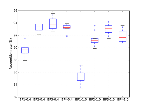
Figure 13: Recognition rates on the test set of the microscopic database, over 10 replications, for lower resolution system with the best results. BP1, BP2, BP3: SLF with LBP and LPQ feature sets combined, with $L$ set to 1, 2 and 3, respectively; BP*: AMLF with LBP and LPQ feature sets combined.

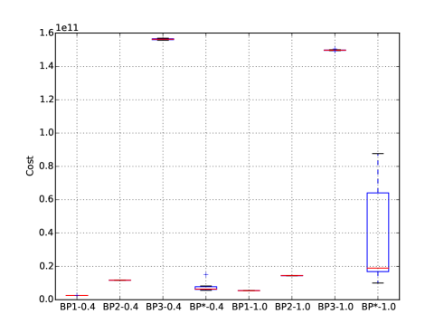
Figure 14: Overall time cost on the test set of the microscopic database, over 10 replications, for lower resolution system with the best results. BP1, BP2, BP3: SLF with LBP and LPQ feature sets combined, with $L$ set to 1, 2 and 3, respectively; BP*: AMLF with LBP and LPQ feature sets combined.

The corresponding recognition rates and costs computed on the macroscopic dataset are presented in Figure 15 and Figure 16. In this case, the impact of global cost reduction is considerably more visible in both aspects. A very significant increase in accuracy is observed with $S=0.1$. In this case, AMLF presents recognition rates of about 96.48%, against 91.86% reached with $S=1.0$. In terms of cost, with $S=0.1$, the average cost of the AMLF can be reduced to about 1/15 of the average cost of AMLF with $S=1.0$. Again, comparing the system with global cost reduction with the system with no reduction at all, the reduction in cost is of about 22 times with much better recognition rates.

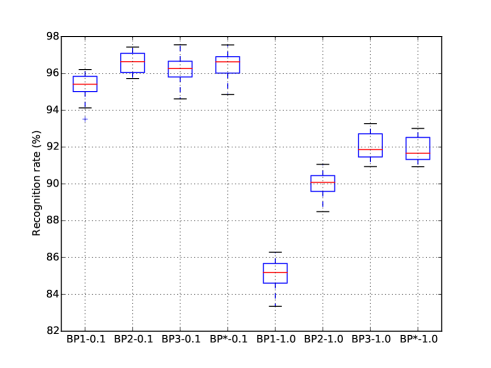
Figure 15: Recognition rates on the test set of the macroscopic database, over 10 replications, for lower resolution system with the best results. BP1, BP2, BP3: SLF with LBP and LPQ feature sets combined, with $L$ set to 1, 2 and 3, respectively; BP*: AMLF with LBP and LPQ feature sets combined.

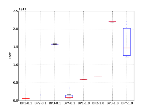
Figure 16: Overall time cost on the test set of the macroscopic database, over 10 replications, for lower resolution system with the best results. BP1, BP2, BP3: SLF with LBP and LPQ feature sets combined, with $L$ set to 1, 2 and 3, respectively; BP*: AMLF with LBP and LPQ feature sets combined.

To conclude these analyses, Figure 17 and Figure 18 present the average percentage of samples recognized at each layer in AMLF, for microscopic and macroscopic respectively. Compared with Figure 5 and Figure 8, we observe that AMLF tends to recognize more samples in the first layer with lower values of $S$, since the versions of SLF with lower values of $L$ are more accurate than those with higher values of $S$. As a consequence, using SLF with $L=1$ for recognizing more samples and in a more accurate way, has a direct impact in reducing the overall cost, while maintaining or even increasing the overall accuracy.

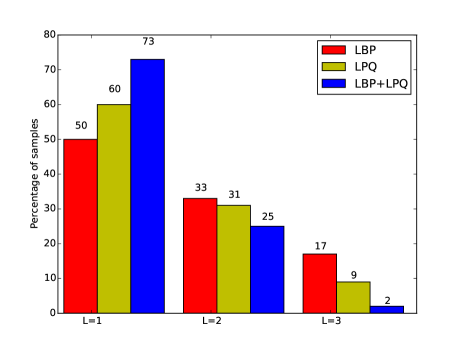
Figure 17: Average percentage of samples recognized at each level of the best configuration of AMLF with LBP, LPQ, and LBP and LPQ combined, respectively, on the microscopic dataset.

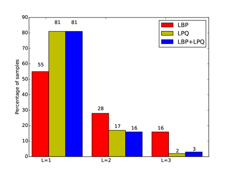
Figure 18: Average percentage of samples recognized at each level of the best configuration of AMLF with LBP, LPQ, and LBP and LPQ combined, respectively, on the macroscopic dataset.

7 Summary of the results

In Table 3 we list the best results achieved in this work, in terms of both recognition accuracy and relative cost (using AMLF with reduced cost as reference), comparing against SLF (with no cost reduction) and the best methods from the literature.

Table 3: Results summary.

	Microscopic dataset		Macroscopic dataset
Method	Accuracy (%)	Cost	Accuracy (%)	Cost
AMLF	93.17	1.0	96.48	1.0
SLF	93.08	20.0	92.81	22.0
Hafemann et al. [6]	97.32	31.2	95.77	1.8
Paula Filho et al. [16]	-	-	97.77	86.7
Kapp et al. [7]	95.68	60.0	88.90	22.0

As observed, AMLF with global cost reduction can result in a system with about or less than 1/20 of the cost of SLF, but achieving better recognition rates in both datasets. Comparing with other methods that achieved better results on the microscopic dataset, we see that the methods presented in [6] and [7] reach recognition rates that are 4.15 and 2.51 percentage points better than AMLF, respectively, but with corresponding costs that are 31.2 and 60.0 times higher. However, neither of those methods outperform AMLF in the macroscopic dataset. On that database, the approach from [16] achieves the best accuracy, which is 1.33 percentage points better than that of AMLF, with a cost that is 86.7 higher. It is worth mentioning, however, that the techniques used by these methods from the literature could also be used with AMLF, which may likely improve its performance.

8 Conclusion and future work

In this paper we investigated ways to reduce costs of forest species recognition systems. We focused on local cost reduction of classification or feature extraction individually, and both combined, i.e. globally.

To reduce costs at classification level, we proposed an adaptive multi-level framework for forest species recognition, based on extending the static single-layer framework proposed in [4]. This approach demonstrated to be able to achieve comparable accuracy to that of the most costly version of SLF, but with about 1/10 of the cost on the microscopic dataset, and 1/3 on macroscopic images.

For feature extraction cost reduction, the simple idea of reducing the resolution of the input image results in linear cost reduction, and in some cases, higher accuracy. With the microscopic dataset, better recognition rates are achieved with only about 40% of the original cost. And on macroscopic images, much better accuracy is observed with the cost reduced to only 10%.

A further evaluation in global cost reduction demonstrated that when AMLF is applied on images with lower resolution, the resulting accuracy can be equivalent or even better than that of SLF, but with the cost reduced by more than 20 times.

As future work, many directions can be followed. One might be improving the proposed AMLF method, and the methods that are used for its set up. For instance, other approaches to define the rejection between sub-sequent layers could be investigated, for instance, class-based thresholds. At feature extraction level, we should also investigate the impact of image resolution reduction with other feature sets to better understand the different scenarios for which this method can be used. Another interesting direction would be the extension of the investigation presented in this work to other texture recognition problems, and other features sets and classifiers, especially Convolutional Neural Networks.

References

- [1] ArunPriya C. and Antony Selvadoss Thanamani. A survey on species recognition system for plant classification. International Journal of Computer Technology & Applications, 3(3):1132–1136, 2012.
- [2] R. Bremananth, B. Nithya B, and R. Saipriya. Wood species recognition system. International Journal of Electrical and Computing Engineering, 4(5):315–321, 2009.
- [3] Paulo R. Cavalin, Marcelo N. Kapp, and Luiz E. S. Oliveira. An adaptive multi-level framework for forest species recognition. In Brazilian Conference on Intelligent Systems, Natal, Brazil, 2015.
- [4] Paulo R. Cavalin, Jefferson Martins, Marcelo N. Kapp, and Luiz E. Oliveira. A multiple feature vector framework for forest species recognition. In The 28th Symposium on Applied Computing, pages 16–20, Coimbra, Portugal, 2013.
- [5] Peter Gasson, Regis Miller, Dov J. Stekel, Frances Whinder, and Kasia Ziemińska. Wood identification of dalbergia nigra (cites appendix i) using quantitative wood anatomy, principal components analysis and naïve bayes classification. Annals of Botany, (105):45–56, 2010.
- [6] Luiz G. Hafemann, Luiz S. Oliveira, and Paulo Cavalin. Forest species recognition using deep convolutional neural networks. In Proceedings of 22nd International Conference on Pattern Recognition (ICPR), 2014 22nd International Conference on Pattern Recognition (ICPR), pages 1103–1107, 2014.
- [7] M. Kapp, R. Bloot, P. R. Cavalin, and L. S. Oliveira. Automatic forest species recognition based on multiple feature sets. In International Joint Conference ou Neural Networks, pages 1296–1303, 2012.
- [8] M. Khalid, E. L. Y. Lee, R. Yusof, and M. Nadaraj. Design of an intelligent wood species recognition system. IJSSST, 9(3), 2008.
- [9] Marzuki Khalid, Rubiyah Yusof, and Anis Salwa Mohd Khairuddin. Tropical wood species recognition system based on multi-feature extractors and classifiers. In 2nd International Conference on Instrumentation Control and Automation, pages 6–11, 2011.
- [10] M. Last, H. Bunke, and A. Kandel. A feature-based serial approach to classifier combination. Pattern Analysis & Applications, 5(4):385–398, 2002.
- [11] J. Martins, L. S. Oliveira, A. S. Britto-Jr, and R. Sabourin. Forest species recognition based on dynamic classifier selection and dissimilarity feature vector representation. Machine Vision and Applications, 26(2):279–293, 2015.
- [12] J. Martins, L. S. Oliveira, and R. Sabourin. Combining textural descriptors for forest species recognition. In 38th Annual Conference of the IEEE Industrial Electronics Society (IECON 2012), 2012.
- [13] J. Martins, L. S. Oliveira, and R. Sabourin. A database for automatic classification of forest species. Machine Vision and Applications, 24(3):567–578, 2013.
- [14] M. Nasirzadeh, A. A. Khazael, and M. B Khalid. Woods recognition system based on local binary pattern. Second International Conference on Computational Intelligence, Communication Systems and Networks, pages 308–313, 2010.
- [15] P. L. Paula Filho, L. S. Oliveira, A. S. Britto, and R. Sabourin. Forest species recognition using color-based features. In Proceedings of the 20th International Conference on Pattern Recognition, pages 4178–4181, Instanbul, Turkey, 2010.
- [16] P. L. Paula Filho, L. S. Oliveira, S. Nisgoski, and A. S. Britto Jr. Forest species recognition using macroscopic images. Machine Vision and Applications, 25(4):1019–1031, 2014.
- [17] J. Y. Tou, P. Y. Lau, and Proceedings of Y. H. Tay. Computer vision-based wood recognition system. In Int. Workshop on Advanced Image Technology, 2007.
- [18] J. Y. Tou, Y. H. Tay, and P. Y. Lau. One-dimensional grey-level co-occurrence matrices for texture classification. International Symposium on Information Technology (ITSim 2008), pages 1–6, 2008.
- [19] Jing Yi Tou, Yong Haur Tay, and Phooi Yee Lau. A comparative study for texture classification techniques on wood recognition problem. In Proceeding of the Fifth International Conference on Natural Computation, pages 8–12, 2009.
- [20] A. R. Yadav, R. S. Anand, M. L. Dewal, and S. Gupta. Multiresolution local binary pattern variants based texture feature extraction techniques for efficient classification of microscopic images of hardwood species. Applied Soft Computing, 32:101–112, 2015.
- [21] A. R. Yadav, M. L. Dewal, R. S. Anand, and S. Gupta. Classification of hardwood species using ann classifier. In National Conference on Computer Vision, Pattern Recognition, Image Processing and Graphics, pages 1–5, 2013.
- [22] R. Yusof, M. Khalid, and A. S. M. Khairuddin. Fuzzy logic-based pre-classifier for tropical wood species recognition system. Machine Vision and Applications, 24(8):1589–1604, 2013.
- [23] Rubiyah Yusof, Nenny Ruthfalydia Rosli, and Marzuki Khalid. Using gabor filters as image multiplier for tropical wood species recognition system. 12th International Conference on Computer Modelling and Simulation, pages 284–289, 2010.